The OctonionsJohn C. Baez

Department of MathematicsUniversity of California

Riverside CA 92521email: baez@math.ucr.edu

May 16, 2001

Abstract

The octonions are the largest of the four normed division algebras. While somewhat neglecteddue to their nonassociativity, they stand at the crossroads of many interesting fields of mathe-matics. Here we describe them and their relation to Clifford algebras and spinors, Bott period-icity, projective and Lorentzian geometry, Jordan algebras, and the exceptional Lie groups. Wealso touch upon their applications in quantum logic, special relativity and supersymmetry.

1 Introduction

There are exactly four normed division algebras: the real numbers (R), complex numbers (C),quaternions (H), and octonions (O). The real numbers are the dependable breadwinner of thefamily, the complete ordered field we all rely on. The complex numbers are a slightly flashier butstill respectable younger brother: not ordered, but algebraically complete. The quaternions, beingnoncommutative, are the eccentric cousin who is shunned at important family gatherings. But theoctonions are the crazy old uncle nobody lets out of the attic: they are nonassociative.

Most mathematicians have heard the story of how Hamilton invented the quaternions. In 1835, atthe age of 30, he had discovered how to treat complex numbers as pairs of real numbers. Fascinatedby the relation between C and 2-dimensional geometry, he tried for many years to invent a biggeralgebra that would play a similar role in 3-dimensional geometry. In modern language, it seems hewas looking for a 3-dimensional normed division algebra. His quest built to its climax in October1843. He later wrote to his son, “Every morning in the early part of the above-cited month, on mycoming down to breakfast, your (then) little brother William Edwin, and yourself, used to ask me:‘Well, Papa, can you multiply triplets?’ Whereto I was always obliged to reply, with a sad shake ofthe head: ‘No, I can only add and subtract them’.” The problem, of course, was that there existsno 3-dimensional normed division algebra. He really needed a 4-dimensional algebra.

Finally, on the 16th of October, 1843, while walking with his wife along the Royal Canal to ameeting of the Royal Irish Academy in Dublin, he made his momentous discovery. “That is to say,I then and there felt the galvanic circuit of thought close; and the sparks which fell from it were thefundamental equations between i, j, k; exactly such as I have used them ever since.” And in a famousact of mathematical vandalism, he carved these equations into the stone of the Brougham Bridge:

i2 = j2 = k2 = ijk = −1.

One reason this story is so well-known is that Hamilton spent the rest of his life obsessed withthe quaternions and their applications to geometry [45, 53]. And for a while, quaternions werefashionable. They were made a mandatory examination topic in Dublin, and in some Americanuniversities they were the only advanced mathematics taught. Much of what we now do with scalarsand vectors in R3 was then done using real and imaginary quaternions. A school of ‘quaternionists’developed, which was led after Hamilton’s death by Peter Tait of Edinburgh and Benjamin Peirce ofHarvard. Tait wrote 8 books on the quaternions, emphasizing their applications to physics. WhenGibbs invented the modern notation for the dot product and cross product, Tait condemned it as a“hermaphrodite monstrosity”. A war of polemics ensued, with such luminaries as Heaviside weighing

1

in on the side of vectors. Ultimately the quaternions lost, and acquired a slight taint of disgracefrom which they have never fully recovered [27].

Less well-known is the discovery of the octonions by Hamilton’s friend from college, John T.Graves. It was Graves’ interest in algebra that got Hamilton thinking about complex numbersand triplets in the first place. The very day after his fateful walk, Hamilton sent an 8-page letterdescribing the quaternions to Graves. Graves replied on October 26th, complimenting Hamilton onthe boldness of the idea, but adding “There is still something in the system which gravels me. I havenot yet any clear views as to the extent to which we are at liberty arbitrarily to create imaginaries,and to endow them with supernatural properties.” And he asked: “If with your alchemy you canmake three pounds of gold, why should you stop there?”

Graves then set to work on some gold of his own! On December 26th, he wrote to Hamiltondescribing a new 8-dimensional algebra, which he called the ‘octaves’. He showed that they were anormed division algebra, and used this to express the product of two sums of eight perfect squaresas another sum of eight perfect squares: the ‘eight squares theorem’ [52].

In January 1844, Graves sent three letters to Hamilton expanding on his discovery. He consideredthe idea of a general theory of ‘2m-ions’, and tried to construct a 16-dimensional normed divisionalgebra, but he “met with an unexpected hitch” and came to doubt that this was possible. Hamiltonoffered to publicize Graves’ discovery, but being busy with work on quaternions, he kept putting itoff. In July he wrote to Graves pointing out that the octonions were nonassociative: “A · BC =AB · C = ABC, if A,B,C be quaternions, but not so, generally, with your octaves.” In fact,Hamilton first invented the term ‘associative’ at about this time, so the octonions may have playeda role in clarifying the importance of this concept.

Meanwhile the young Arthur Cayley, fresh out of Cambridge, had been thinking about thequaternions ever since Hamilton announced their existence. He seemed to be seeking relationshipsbetween the quaternions and hyperelliptic functions. In March of 1845, he published a paper in thePhilosophical Magazine entitled ‘On Jacobi’s Elliptic Functions, in Reply to the Rev. B. Bronwin;and on Quaternions’ [18]. The bulk of this paper was an attempt to rebut an article pointing outmistakes in Cayley’s work on elliptic functions. Apparently as an afterthought, he tacked on a briefdescription of the octonions. In fact, this paper was so full of errors that it was omitted from hiscollected works — except for the part about octonions [19].

Upset at being beaten to publication, Graves attached a postscript to a paper of his own whichwas to appear in the following issue of the same journal, saying that he had known of the octonionsever since Christmas, 1843. On June 14th, 1847, Hamilton contributed a short note to the Transac-tions of the Royal Irish Academy, vouching for Graves’ priority. But it was too late: the octonionsbecame known as ‘Cayley numbers’. Still worse, Graves later found that his eight squares theoremhad already been discovered by C. F. Degen in 1818 [28, 30].

Why have the octonions languished in such obscurity compared to the quaternions? Besidestheir rather inglorious birth, one reason is that they lacked a tireless defender such as Hamilton.But surely the reason for this is that they lacked any clear application to geometry and physics.The unit quaternions form the group SU(2), which is the double cover of the rotation group SO(3).This makes them nicely suited to the study of rotations and angular momentum, particularly inthe context of quantum mechanics. These days we regard this phenomenon as a special case of thetheory of Clifford algebras. Most of us no longer attribute to the quaternions the cosmic significancethat Hamilton claimed for them, but they fit nicely into our understanding of the scheme of things.

The octonions, on the other hand, do not. Their relevance to geometry was quite obscureuntil 1925, when Elie Cartan described ‘triality’ — the symmetry between vectors and spinors in 8-dimensional Euclidean space [17]. Their potential relevance to physics was noticed in a 1934 paper byJordan, von Neumann and Wigner on the foundations of quantum mechanics [59]. However, attemptsby Jordan and others to apply octonionic quantum mechanics to nuclear and particle physics metwith little success. Work along these lines continued quite slowly until the 1980s, when it wasrealized that the octonions explain some curious features of string theory [65]. The Lagrangian for

2

the classical superstring involves a relationship between vectors and spinors in Minkowski spacetimewhich holds only in 3, 4, 6, and 10 dimensions. Note that these numbers are 2 more than thedimensions of R,C,H and O. As we shall see, this is no coincidence: briefly, the isomorphisms

sl(2,R) ∼= so(2, 1)sl(2,C) ∼= so(3, 1)sl(2,H) ∼= so(5, 1)sl(2,O) ∼= so(9, 1)

allow us to treat a spinor in one of these dimensions as a pair of elements of the corresponding divisionalgebra. It is fascinating that of these superstring Lagrangians, it is the 10-dimensional octonionicone that gives the most promising candidate for a realistic theory of fundamental physics! However,there is still no proof that the octonions are useful for understanding the real world. We can onlyhope that eventually this question will be settled one way or another.

Besides their possible role in physics, the octonions are important because they tie togethersome algebraic structures that otherwise appear as isolated and inexplicable exceptions. As weshall explain, the concept of an octonionic projective space OPn only makes sense for n ≤ 2, dueto the nonassociativity of O. This means that various structures associated to real, complex andquaternionic projective spaces have octonionic analogues only for n ≤ 2.

Simple Lie algebras are a nice example of this phenomenon. There are 3 infinite families of‘classical’ simple Lie algebras, which come from the isometry groups of the projective spaces RPn,CPn and HPn. There are also 5 ‘exceptional’ simple Lie algebras. These were discovered by Killingand Cartan in the late 1800s. At the time, the significance of these exceptions was shrouded inmystery: they did not arise as symmetry groups of known structures. Only later did their connectionto the octonions become clear. It turns out that 4 of them come from the isometry groups of theprojective planes over O, O⊗C, O⊗H and O⊗O. The remaining one is the automorphism groupof the octonions!

Another good example is the classification of simple formally real Jordan algebras. Besidesseveral infinite families of these, there is the ‘exceptional’ Jordan algebra, which consists of 3 × 3hermitian octonionic matrices. Minimal projections in this Jordan algebra correspond to points ofOP2, and the automorphism group of this algebra is the same as the isometry group of OP2.

The octonions also have fascinating connections to topology. In 1957, Raoul Bott computedthe homotopy groups of the topological group O(∞), which is the inductive limit of the orthogonalgroups O(n) as n→∞. He proved that they repeat with period 8:

πi+8(O(∞)) ∼= πi(O(∞)).

This is known as ‘Bott periodicity’. He also computed the first 8:

π0(O(∞)) ∼= Z2

π1(O(∞)) ∼= Z2

π2(O(∞)) ∼= 0

π3(O(∞)) ∼= Zπ4(O(∞)) ∼= 0

π5(O(∞)) ∼= 0

π6(O(∞)) ∼= 0

π7(O(∞)) ∼= Z

Note that the nonvanishing homotopy groups here occur in dimensions one less than the dimensionsof R,C,H, and O. This is no coincidence! In a normed division algebra, left multiplication by anelement of norm one defines an orthogonal transformation of the algebra, and thus an element of

3

O(∞). This gives us maps from the spheres S0, S1, S3 and S7 to O(∞), and these maps generatethe homotopy groups in those dimensions.

Given this, one might naturally guess that the period-8 repetition in the homotopy groups ofO(∞) is in some sense ‘caused’ by the octonions. As we shall see, this is true. Conversely, Bottperiodicity is closely connected to the problem of how many pointwise linearly independent smoothvector fields can be found on the n-sphere [56]. There exist n such vector fields only when n+ 1 =1, 2, 4, or 8, and this can be used to show that division algebras over the reals can only occur inthese dimensions.

In what follows we shall try to explain the octonions and their role in algebra, geometry, andtopology. In Section 2 we give four constructions of the octonions: first via their multiplicationtable, then using the Fano plane, then using the Cayley–Dickson construction and finally usingClifford algebras, spinors, and a generalized concept of ‘triality’ advocated by Frank Adams [2].Each approach has its own merits. In Section 3 we discuss the projective lines and planes overthe normed division algebras — especially O — and describe their relation to Bott periodicity, theexceptional Jordan algebra, and the Lie algebra isomorphisms listed above. Finally, in Section 4 wediscuss octonionic constructions of the exceptional Lie groups, especially the ‘magic square’.

1.1 Preliminaries

Before our tour begins, let us settle on some definitions. For us a vector space will always be afinite-dimensional module over the field of real numbers. An algebra A will be a vector space thatis equipped with a bilinear map m:A×A→ A called ‘multiplication’ and a nonzero element 1 ∈ Acalled the ‘unit’ such that m(1, a) = m(a, 1) = a. As usual, we abbreviate m(a, b) as ab. We donot assume our algebras are associative! Given an algebra, we will freely think of real numbers aselements of this algebra via the map α 7→ α1.

An algebra A is a division algebra if given a, b ∈ A with ab = 0, then either a = 0 or b = 0.Equivalently, A is a division algebra if the operations of left and right multiplication by any nonzeroelement are invertible. A normed division algebra is an algebra A that is also a normed vectorspace with ‖ab‖ = ‖a‖‖b‖. This implies that A is a division algebra and that ‖1‖ = 1.

We should warn the reader of some subtleties. We say an algebra A has multiplicative inversesif for any nonzero a ∈ A there is an element a−1 ∈ A with aa−1 = a−1a = 1. An associative algebrahas multiplicative inverses iff it is a division algebra. However, this fails for nonassociative algebras!In Section 2.2 we shall construct algebras that have multiplicative inverses, but are not divisionalgebras. On the other hand, we can construct a division algebra without multiplicative inversesby taking the quaternions and modifying the product slightly, setting i2 = −1 + εj for some smallnonzero real number ε while leaving the rest of the multiplication table unchanged. The elementi then has both right and left inverses, but they are not equal. (We thank David Rusin for thisexample.)

There are three levels of associativity. An algebra is power-associative if the subalgebra gen-erated by any one element is associative. It is alternative if the subalgebra generated by any twoelements is associative. Finally, if the subalgebra generated by any three elements is associative, thealgebra is associative.

As we shall see, the octonions are not associative, but they are alternative. How does one checka thing like this? By a theorem of Emil Artin [84], an algebra A is alternative iff for all a, b ∈ A wehave

(aa)b = a(ab), (ab)a = a(ba), (ba)a = b(aa) (1)

In fact, any two of these equations implies the remaining one, so people usually take the first andlast as the definition of ‘alternative’. To see this fact, note that any algebra has a trilinear map

[·, ·, ·]:A3 → A

4

called the associator, given by[a, b, c] = (ab)c− a(bc).

The associator measures the failure of associativity just as the commutator [a, b] = ab− ba measuresthe failure of commutativity. Now, the commutator is an alternating bilinear map, meaning that itswitches sign whenever the two arguments are exchanged:

[a, b] = −[b, a]

or equivalently, that it vanishes when they are equal:

[a, a] = 0.

This raises the question of whether the associator is alternating too. In fact, this holds preciselywhen A is alternative! The reason is that each equation in (1) says that the associator vanisheswhen a certain pair of arguments are equal, or equivalently, that it changes sign when that pair ofarguments is switched. Note, however, that if the associator changes sign when we switch the ithand jth arguments, and also when we switch the jth and kth arguments, it must change sign whenwe switch the ith and kth. Thus any two of equations (1) imply the third.

Now we can say what is so great about R,C,H, and O:

Theorem 1. R,C,H, and O are the only normed division algebras.

Theorem 2. R,C,H, and O are the only alternative division algebras.

The first theorem goes back to an 1898 paper by Hurwitz [55]. It was subsequently generalizedin many directions, for example, to algebras over other fields. A version of the second theoremappears in an 1930 paper by Zorn [100] — the guy with the lemma. For modern proofs of both thesetheorems, see Schafer’s excellent book on nonassociative algebras [84]. We sketch a couple proofs ofHurwitz’s theorem in Section 2.3.

Note that we did not state that R,C,H and O are the only division algebras. This is not true.For example, we have already described a way to get 4-dimensional division algebras that do nothave multiplicative inverses. However, we do have this fact:

Theorem 3. All division algebras have dimension 1, 2, 4, or 8.

This was independently proved by Kervaire [62] and Bott–Milnor [11] in 1958. We will say a bitabout the proof in Section 3.1. However, in what follows our main focus will not be on generalresults about division algebras. Instead, we concentrate on special features of the octonions. Let usbegin by constructing them.

2 Constructing the Octonions

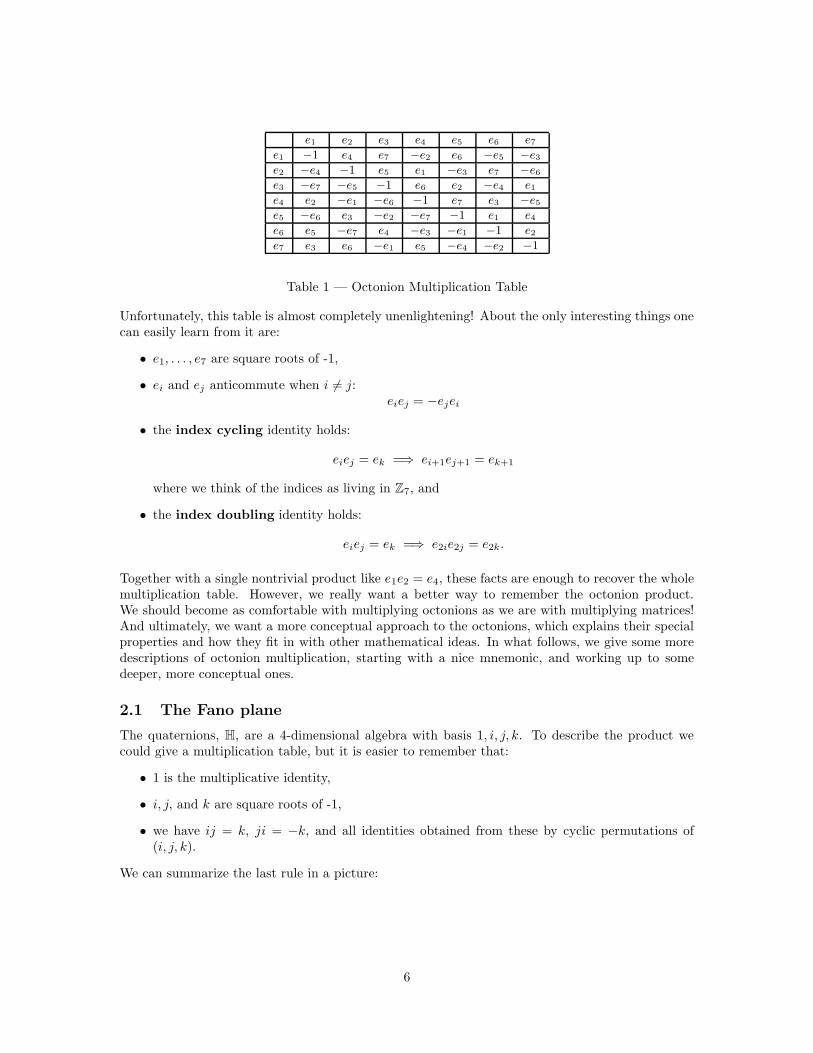
The most elementary way to construct the octonions is to give their multiplication table. Theoctonions are an 8-dimensional algebra with basis 1, e1, e2, e3, e4, e5, e6, e7, and their multiplicationis given in this table, which describes the result of multiplying the element in the ith row by theelement in the jth column:

5

e1 e2 e3 e4 e5 e6 e7

e1 −1 e4 e7 −e2 e6 −e5 −e3

e2 −e4 −1 e5 e1 −e3 e7 −e6

e3 −e7 −e5 −1 e6 e2 −e4 e1

e4 e2 −e1 −e6 −1 e7 e3 −e5

e5 −e6 e3 −e2 −e7 −1 e1 e4

e6 e5 −e7 e4 −e3 −e1 −1 e2

e7 e3 e6 −e1 e5 −e4 −e2 −1

Table 1 — Octonion Multiplication Table

Unfortunately, this table is almost completely unenlightening! About the only interesting things onecan easily learn from it are:

• e1, . . . , e7 are square roots of -1,

• ei and ej anticommute when i 6= j:eiej = −ejei

• the index cycling identity holds:

eiej = ek =⇒ ei+1ej+1 = ek+1

where we think of the indices as living in Z7, and

• the index doubling identity holds:

eiej = ek =⇒ e2ie2j = e2k.

Together with a single nontrivial product like e1e2 = e4, these facts are enough to recover the wholemultiplication table. However, we really want a better way to remember the octonion product.We should become as comfortable with multiplying octonions as we are with multiplying matrices!And ultimately, we want a more conceptual approach to the octonions, which explains their specialproperties and how they fit in with other mathematical ideas. In what follows, we give some moredescriptions of octonion multiplication, starting with a nice mnemonic, and working up to somedeeper, more conceptual ones.

2.1 The Fano plane

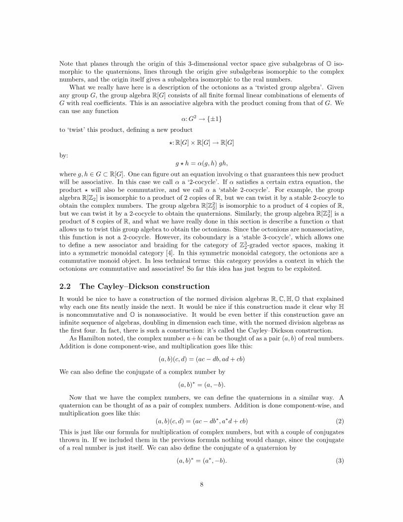
The quaternions, H, are a 4-dimensional algebra with basis 1, i, j, k. To describe the product wecould give a multiplication table, but it is easier to remember that:

• 1 is the multiplicative identity,

• i, j, and k are square roots of -1,

• we have ij = k, ji = −k, and all identities obtained from these by cyclic permutations of(i, j, k).

We can summarize the last rule in a picture:

6

k

i

j

When we multiply two elements going clockwise around the circle we get the next one: for example,ij = k. But when we multiply two going around counterclockwise, we get minus the next one: forexample, ji = −k.

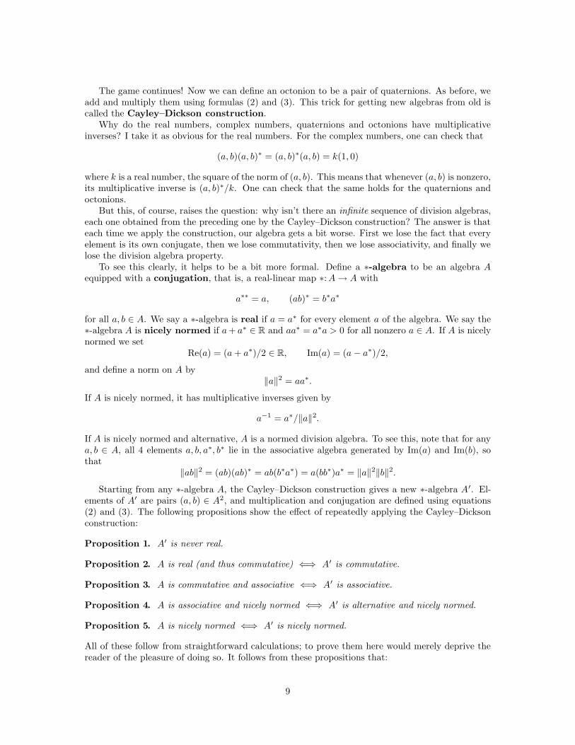
We can use the same sort of picture to remember how to multiply octonions:

i

e4

e3 e

e7

e1

e52

e6

This is the Fano plane, a little gadget with 7 points and 7 lines. The ‘lines’ are the sides of thetriangle, its altitudes, and the circle containing all the midpoints of the sides. Each pair of distinctpoints lies on a unique line. Each line contains three points, and each of these triples has has a cyclicordering shown by the arrows. If ei, ej , and ek are cyclically ordered in this way then

eiej = ek, ejei = −ek.

Together with these rules:

• 1 is the multiplicative identity,

• e1, . . . , e7 are square roots of -1,

the Fano plane completely describes the algebra structure of the octonions. Index-doubling corre-sponds to rotating the picture a third of a turn.

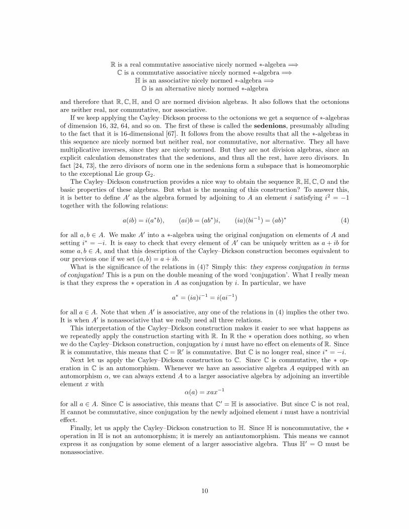
This is certainly a neat mnemonic, but is there anything deeper lurking behind it? Yes! TheFano plane is the projective plane over the 2-element field Z2. In other words, it consists of linesthrough the origin in the vector space Z3

2. Since every such line contains a single nonzero element,we can also think of the Fano plane as consisting of the seven nonzero elements of Z3

2. If we thinkof the origin in Z3

2 as corresponding to 1 ∈ O, we get the following picture of the octonions:

1

e4

e3

e2

e5

e

e6

e7

1

7

Note that planes through the origin of this 3-dimensional vector space give subalgebras of O iso-morphic to the quaternions, lines through the origin give subalgebras isomorphic to the complexnumbers, and the origin itself gives a subalgebra isomorphic to the real numbers.

What we really have here is a description of the octonions as a ‘twisted group algebra’. Givenany group G, the group algebra R[G] consists of all finite formal linear combinations of elements ofG with real coefficients. This is an associative algebra with the product coming from that of G. Wecan use any function

α:G2 → {±1}to ‘twist’ this product, defining a new product

?:R[G]× R[G]→ R[G]

by:g ? h = α(g, h) gh,

where g, h ∈ G ⊂ R[G]. One can figure out an equation involving α that guarantees this new productwill be associative. In this case we call α a ‘2-cocycle’. If α satisfies a certain extra equation, theproduct ? will also be commutative, and we call α a ‘stable 2-cocycle’. For example, the groupalgebra R[Z2] is isomorphic to a product of 2 copies of R, but we can twist it by a stable 2-cocyle toobtain the complex numbers. The group algebra R[Z2

2] is isomorphic to a product of 4 copies of R,but we can twist it by a 2-cocycle to obtain the quaternions. Similarly, the group algebra R[Z3

2] is aproduct of 8 copies of R, and what we have really done in this section is describe a function α thatallows us to twist this group algebra to obtain the octonions. Since the octonions are nonassociative,this function is not a 2-cocycle. However, its coboundary is a ‘stable 3-cocycle’, which allows oneto define a new associator and braiding for the category of Z3

2-graded vector spaces, making itinto a symmetric monoidal category [4]. In this symmetric monoidal category, the octonions are acommutative monoid object. In less technical terms: this category provides a context in which theoctonions are commutative and associative! So far this idea has just begun to be exploited.

2.2 The Cayley–Dickson construction

It would be nice to have a construction of the normed division algebras R,C,H,O that explainedwhy each one fits neatly inside the next. It would be nice if this construction made it clear why His noncommutative and O is nonassociative. It would be even better if this construction gave aninfinite sequence of algebras, doubling in dimension each time, with the normed division algebras asthe first four. In fact, there is such a construction: it’s called the Cayley–Dickson construction.

As Hamilton noted, the complex number a+bi can be thought of as a pair (a, b) of real numbers.Addition is done component-wise, and multiplication goes like this:

(a, b)(c, d) = (ac− db, ad+ cb)

We can also define the conjugate of a complex number by

(a, b)∗ = (a,−b).

Now that we have the complex numbers, we can define the quaternions in a similar way. Aquaternion can be thought of as a pair of complex numbers. Addition is done component-wise, andmultiplication goes like this:

(a, b)(c, d) = (ac− db∗, a∗d+ cb) (2)

This is just like our formula for multiplication of complex numbers, but with a couple of conjugatesthrown in. If we included them in the previous formula nothing would change, since the conjugateof a real number is just itself. We can also define the conjugate of a quaternion by

(a, b)∗ = (a∗,−b). (3)

8

The game continues! Now we can define an octonion to be a pair of quaternions. As before, weadd and multiply them using formulas (2) and (3). This trick for getting new algebras from old iscalled the Cayley–Dickson construction.

Why do the real numbers, complex numbers, quaternions and octonions have multiplicativeinverses? I take it as obvious for the real numbers. For the complex numbers, one can check that

(a, b)(a, b)∗ = (a, b)∗(a, b) = k(1, 0)

where k is a real number, the square of the norm of (a, b). This means that whenever (a, b) is nonzero,its multiplicative inverse is (a, b)∗/k. One can check that the same holds for the quaternions andoctonions.

But this, of course, raises the question: why isn’t there an infinite sequence of division algebras,each one obtained from the preceding one by the Cayley–Dickson construction? The answer is thateach time we apply the construction, our algebra gets a bit worse. First we lose the fact that everyelement is its own conjugate, then we lose commutativity, then we lose associativity, and finally welose the division algebra property.

To see this clearly, it helps to be a bit more formal. Define a ∗-algebra to be an algebra Aequipped with a conjugation, that is, a real-linear map ∗:A→ A with

a∗∗ = a, (ab)∗ = b∗a∗

for all a, b ∈ A. We say a ∗-algebra is real if a = a∗ for every element a of the algebra. We say the∗-algebra A is nicely normed if a+ a∗ ∈ R and aa∗ = a∗a > 0 for all nonzero a ∈ A. If A is nicelynormed we set

Re(a) = (a+ a∗)/2 ∈ R, Im(a) = (a− a∗)/2,and define a norm on A by

‖a‖2 = aa∗.

If A is nicely normed, it has multiplicative inverses given by

a−1 = a∗/‖a‖2.

If A is nicely normed and alternative, A is a normed division algebra. To see this, note that for anya, b ∈ A, all 4 elements a, b, a∗, b∗ lie in the associative algebra generated by Im(a) and Im(b), sothat

‖ab‖2 = (ab)(ab)∗ = ab(b∗a∗) = a(bb∗)a∗ = ‖a‖2‖b‖2.Starting from any ∗-algebra A, the Cayley–Dickson construction gives a new ∗-algebra A′. El-

ements of A′ are pairs (a, b) ∈ A2, and multiplication and conjugation are defined using equations(2) and (3). The following propositions show the effect of repeatedly applying the Cayley–Dicksonconstruction:

Proposition 1. A′ is never real.

Proposition 2. A is real (and thus commutative) ⇐⇒ A′ is commutative.

Proposition 3. A is commutative and associative ⇐⇒ A′ is associative.

Proposition 4. A is associative and nicely normed ⇐⇒ A′ is alternative and nicely normed.

Proposition 5. A is nicely normed ⇐⇒ A′ is nicely normed.

All of these follow from straightforward calculations; to prove them here would merely deprive thereader of the pleasure of doing so. It follows from these propositions that:

9

R is a real commutative associative nicely normed ∗-algebra =⇒C is a commutative associative nicely normed ∗-algebra =⇒

H is an associative nicely normed ∗-algebra =⇒O is an alternative nicely normed ∗-algebra

and therefore that R,C,H, and O are normed division algebras. It also follows that the octonionsare neither real, nor commutative, nor associative.

If we keep applying the Cayley–Dickson process to the octonions we get a sequence of ∗-algebrasof dimension 16, 32, 64, and so on. The first of these is called the sedenions, presumably alludingto the fact that it is 16-dimensional [67]. It follows from the above results that all the ∗-algebras inthis sequence are nicely normed but neither real, nor commutative, nor alternative. They all havemultiplicative inverses, since they are nicely normed. But they are not division algebras, since anexplicit calculation demonstrates that the sedenions, and thus all the rest, have zero divisors. Infact [24, 73], the zero divisors of norm one in the sedenions form a subspace that is homeomorphicto the exceptional Lie group G2.

The Cayley–Dickson construction provides a nice way to obtain the sequence R,H,C,O and thebasic properties of these algebras. But what is the meaning of this construction? To answer this,it is better to define A′ as the algebra formed by adjoining to A an element i satisfying i2 = −1together with the following relations:

a(ib) = i(a∗b), (ai)b = (ab∗)i, (ia)(bi−1) = (ab)∗ (4)

for all a, b ∈ A. We make A′ into a ∗-algebra using the original conjugation on elements of A andsetting i∗ = −i. It is easy to check that every element of A′ can be uniquely written as a + ib forsome a, b ∈ A, and that this description of the Cayley–Dickson construction becomes equivalent toour previous one if we set (a, b) = a+ ib.

What is the significance of the relations in (4)? Simply this: they express conjugation in termsof conjugation! This is a pun on the double meaning of the word ‘conjugation’. What I really meanis that they express the ∗ operation in A as conjugation by i. In particular, we have

a∗ = (ia)i−1 = i(ai−1)

for all a ∈ A. Note that when A′ is associative, any one of the relations in (4) implies the other two.It is when A′ is nonassociative that we really need all three relations.

This interpretation of the Cayley–Dickson construction makes it easier to see what happens aswe repeatedly apply the construction starting with R. In R the ∗ operation does nothing, so whenwe do the Cayley–Dickson construction, conjugation by i must have no effect on elements of R. SinceR is commutative, this means that C = R′ is commutative. But C is no longer real, since i∗ = −i.

Next let us apply the Cayley–Dickson construction to C. Since C is commutative, the ∗ op-eration in C is an automorphism. Whenever we have an associative algebra A equipped with anautomorphism α, we can always extend A to a larger associative algebra by adjoining an invertibleelement x with

α(a) = xax−1

for all a ∈ A. Since C is associative, this means that C′ = H is associative. But since C is not real,H cannot be commutative, since conjugation by the newly adjoined element i must have a nontrivialeffect.

Finally, let us apply the Cayley–Dickson construction to H. Since H is noncommutative, the ∗operation in H is not an automorphism; it is merely an antiautomorphism. This means we cannotexpress it as conjugation by some element of a larger associative algebra. Thus H′ = O must benonassociative.

10

2.3 Clifford Algebras

William Clifford invented his algebras in 1876 as an attempt to generalize the quaternions to higherdimensions, and he published a paper about them two years later [23]. Given a real inner productspace V , the Clifford algebra Cliff(V ) is the associative algebra freely generated by V modulo therelations

v2 = −‖v‖2

for all v ∈ V . Equivalently, it is the associative algebra freely generated by V modulo the relations

vw + wv = −2〈v, w〉

for all v, w ∈ V . If V = Rn with its usual inner product, we call this Clifford algebra Cliff(n).Concretely, this is the associative algebra freely generated by n anticommuting square roots of −1.From this we easily see that

Cliff(0) = R, Cliff(1) = C, Cliff(2) = H.

So far this sequence resembles the iterated Cayley-Dickson construction — but the octonions are nota Clifford algebra, since they are nonassociative. Nonetheless, there is a profound relation betweenClifford algebras and normed division algebras. This relationship gives a nice way to prove thatR,C,H and O are the only normed dvivision algebras. It is also crucial for understanding thegeometrical meaning of the octonions.

To see this relation, first suppose K is a normed division algebra. Left multiplication by anyelement a ∈ K gives an operator

La : K → Kx 7→ ax.

If ‖a‖ = 1, the operator La is norm-preserving, so it maps the unit sphere of K to itself. Since Kis a division algebra, we can find an operator of this form mapping any point on the unit sphere toany other point. The only way the unit sphere in K can have this much symmetry is if the normon K comes from an inner product. Even better, this inner product is unique, since we can use thepolarization identity

〈x, y〉 =1

2(‖x+ y‖2 − ‖x‖2 − ‖y‖2)

to recover it from the norm.Using this inner product, we say an element a ∈ K is imaginary if it is orthogonal to the element

1, and we let Im(K) be the space of imaginary elements of K. We can also think of Im(K) as thetangent space of the unit sphere in K at the point 1. This has a nice consequence: since a 7→ Lamaps the unit sphere in K to the Lie group of orthogonal transformations of K, it must send Im(K)to the Lie algebra of skew-adjoint transformations of K. In short, La is skew-adjoint whenever a isimaginary.

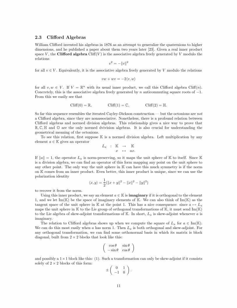
The relation to Clifford algebras shows up when we compute the square of La for a ∈ Im(K).We can do this most easily when a has norm 1. Then La is both orthogonal and skew-adjoint. Forany orthogonal transformation, we can find some orthonormal basis in which its matrix is blockdiagonal, built from 2× 2 blocks that look like this:

(cos θ sin θ− sin θ cos θ

)

and possibly a 1×1 block like this: (1). Such a transformation can only be skew-adjoint if it consistssolely of 2× 2 blocks of this form:

±(

0 1−1 0

).

11

In this case, its square is −1. We thus have L2a = −1 when a ∈ Im(K) has norm 1. It follows that

L2a = −‖a‖2

for all a ∈ Im(K). We thus obtain a representation of the Clifford algebra Cliff(Im(K)) on K. Anyn-dimensional normed division algebra thus gives an n-dimensional representation of Cliff(n − 1).As we shall see, this is very constraining.

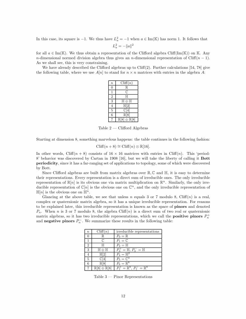
We have already described the Clifford algebras up to Cliff(2). Further calculations [54, 78] givethe following table, where we use A[n] to stand for n× n matrices with entries in the algebra A:

n Cliff(n)

0 R1 C2 H3 H⊕H4 H[2]

5 C[4]

6 R[8]

7 R[8] ⊕ R[8]

Table 2 — Clifford Algebras

Starting at dimension 8, something marvelous happens: the table continues in the following fashion:

Cliff(n+ 8) ∼= Cliff(n)⊗ R[16].

In other words, Cliff(n + 8) consists of 16 × 16 matrices with entries in Cliff(n). This ‘period-8’ behavior was discovered by Cartan in 1908 [16], but we will take the liberty of calling it Bottperiodicity, since it has a far-ranging set of applications to topology, some of which were discoveredby Bott.

Since Clifford algebras are built from matrix algebras over R,C and H, it is easy to determinetheir representations. Every representation is a direct sum of irreducible ones. The only irreduciblerepresentation of R[n] is its obvious one via matrix multiplication on Rn. Similarly, the only irre-ducible representation of C[n] is the obvious one on Cn, and the only irreducible representation ofH[n] is the obvious one on Hn.

Glancing at the above table, we see that unless n equals 3 or 7 modulo 8, Cliff(n) is a real,complex or quaternionic matrix algebra, so it has a unique irreducible representation. For reasonsto be explained later, this irreducible representation is known as the space of pinors and denotedPn. When n is 3 or 7 modulo 8, the algebra Cliff(n) is a direct sum of two real or quaternionicmatrix algebras, so it has two irreducible representations, which we call the positive pinors P+

n

and negative pinors P−n . We summarize these results in the following table:

n Cliff(n) irreducible representations

0 R P0 = R1 C P1 = C2 H P2 = H3 H⊕H P+

3 = H, P−3 = H4 H[2] P4 = H2

5 C[4] P5 = C4

6 R[8] P6 = R8

7 R[8] ⊕ R[8] P+7 = R8, P−7 = R8

Table 3 — Pinor Representations

12

Examining this table, we see that in the range of dimensions listed there is an n-dimensional rep-resentation of Cliff(n − 1) only for n = 1, 2, 4, and 8. What about higher dimensions? By Bottperiodicity, the irreducible representations of Cliff(n+ 8) are obtained by tensoring those of Cliff(n)by R16. This multiplies the dimension by 16, so one can easily check that for n > 8, the irreduciblerepresentations of Cliff(n− 1) always have dimension greater than n.

It follows that normed division algebras are only possible in dimensions 1, 2, 4, and 8. Havingconstructed R,C,H and O, we also know that normed division algebras exist in these dimensions.The only remaining question is whether they are unique. For this it helps to investigate more deeplythe relation between normed division algebras and the Cayley-Dickson construction. In what follows,we outline an approach based on ideas in the book by Springer and Veldkamp [90].

First, suppose K is a normed division algebra. Then there is a unique linear operator ∗:K→ Ksuch that 1∗ = 1 and a∗ = −a for a ∈ Im(K). With some calculation one can prove this makes Kinto a nicely normed ∗-algebra.

Next, suppose that K0 is any subalgebra of the normed division algebra K. It is easy to checkthat K0 is a nicely normed ∗-algebra in its own right. If K0 is not all of K, we can find an elementi ∈ K that is orthogonal to every element of K0. Without loss of generality we shall assume thiselement has norm 1. Since this element i is orthogonal to 1 ∈ K0, it is imaginary. From the definitionof the ∗ operator it follows that i∗ = −i, and from results earlier in this section we have i2 = −1.With further calculation one can show that for all a, a′ ∈ K0 we have

a(ia′) = i(a∗a′), (ai)a′ = (aa′∗)i, (ia)(a′i−1) = (aa′)∗

A glance at equation (4) reveals that these are exactly the relations defining the Cayley-Dicksonconstruction! With a little thought, it follows that the subalgebra of K generated by K0 and i isisomorphic as a ∗-algebra to K′0, the ∗-algebra obtained from K0 by the Cayley-Dickson construction.

Thus, whenever we have a normed division algebra K we can find a chain of subalgebras R =K0 ⊂ K1 ⊂ · · · ⊂ Kn = K such that Ki+1

∼= K′i. To construct Ki+1, we simply need to choose anorm-one element of K that is orthogonal to every element of Ki. It follows that the only normeddivision algebras of dimension 1, 2, 4 and 8 are R,C,H and O. This also gives an alternate proofthat there are no normed division algebras of other dimensions: if there were any, there would haveto be a 16-dimensional one, namely O′ — the sedenions. But as mentioned in Section 2.2, one cancheck explicitly that the sedenions are not a division algebra.

2.4 Spinors and Trialities

A nonassociative division algebra may seem like a strange thing to bother with, but the notion oftriality makes it seem a bit more natural. The concept of duality is important throughout linearalgebra. The concept of triality is similar, but considerably subtler. Given vector spaces V1 and V2,we may define a duality to be a bilinear map

f :V1 × V2 → R

that is nondegenerate, meaning that if we fix either argument to any nonzero value, the linearfunctional induced on the other vector space is nonzero. Similarly, given vector spaces V1, V2, andV3, a triality is a trilinear map

t:V1 × V2 × V3 → R

that is nondegenerate in the sense that if we fix any two arguments to any nonzero values, the linearfunctional induced on the third vector space is nonzero.

Dualities are easy to come by. Trialities are much rarer. For suppose we have a triality

t:V1 × V2 × V3 → R.

13

By dualizing, we can turn this into a bilinear map

m:V1 × V2 → V ∗3

which we call ‘multiplication’. By the nondegeneracy of our triality, left multiplication by anynonzero element of V1 defines an isomorphism from V2 to V ∗3 . Similarly, right multiplication by anynonzero element of V2 defines an isomorphism from V1 to V ∗3 . If we choose nonzero elements e1 ∈ V1

and e2 ∈ V2, we can thereby identify the spaces V1, V2 and V ∗3 with a single vector space, say V .Note that this identifies all three vectors e1 ∈ V1, e2 ∈ V2, and e1e2 ∈ V ∗3 with the same vectore ∈ V . We thus obtain a product

m:V × V → V

for which e is the left and right unit. Since left or right multiplication by any nonzero element is anisomorphism, V is actually a division algebra! Conversely, any division algebra gives a triality.

It follows from Theorem 3 that trialities only occur in dimensions 1, 2, 4, or 8. This theoremis quite deep. By comparison, Hurwitz’s classification of normed division algebras is easy to prove.Not surprisingly, these correspond to a special sort of triality, which we call a ‘normed’ triality.

To be precise, a normed triality consists of inner product spaces V1, V2, V3 equipped with atrilinear map t:V1 × V2 × V3 → R with

|t(v1, v2, v3)| ≤ ‖v1‖ ‖v2‖ ‖v3‖,

and such that for all v1, v2 there exists v3 6= 0 for which this bound is attained — and similarly forcyclic permutations of 1, 2, 3. Given a normed triality, picking unit vectors in any two of the spacesVi allows us to identify all three spaces and get a normed division algebra. Conversely, any normeddivision algebra gives a normed triality.

But where do normed trialities come from? They come from the theory of spinors! FromSection 2.3, we already know that any n-dimensional normed division algebra is a representationof Cliff(n − 1), so it makes sense to look for normed trialities here. In fact, representations ofCliff(n − 1) give certain representations of Spin(n), the double cover of the rotation group in ndimensions. These are called ‘spinors’. As we shall see, the relation between spinors and vectorsgives a nice way to construct normed trialities in dimensions 1, 2, 4 and 8.

To see how this works, first let Pin(n) be the group sitting inside Cliff(n) that consists of allproducts of unit vectors in Rn. This group is a double cover of the orthogonal group O(n), wheregiven any unit vector v ∈ Rn, we map both ±v ∈ Pin(n) to the element of O(n) that reflects acrossthe hyperplane perpendicular to v. Since every element of O(n) is a product of reflections, thishomomorphism is indeed onto.

Next, let Spin(n) ⊂ Pin(n) be the subgroup consisting of all elements that are a product of aneven number of unit vectors in Rn. An element of O(n) has determinant 1 iff it is the product of aneven number of reflections, so just as Pin(n) is a double cover of O(n), Spin(n) is a double cover ofSO(n). Together with a French dirty joke which we shall not explain, this analogy is the origin ofthe terms ‘Pin’ and ‘pinor’.

Since Pin(n) sits inside Cliff(n), the irreducible representations of Cliff(n) restrict to representa-tions of Pin(n), which turn out to be still irreducible. These are again called pinors, and we knowwhat they are from Table 3. Similarly, Spin(n) sits inside the subalgebra

Cliff0(n) ⊆ Cliff(n)

consisting of all linear combinations of products of an even number of vectors in Rn. Thus theirreducible representations of Cliff0(n) restrict to representations of Spin(n), which turn out to bestill irreducible. These are called spinors — but we warn the reader that this term is also used formany slight variations on this concept.

14

In fact, there is an isomorphism

φ: Cliff(n− 1)→ Cliff0(n)

given as follows:φ(ei) = eien, 1 ≤ i ≤ n− 1,

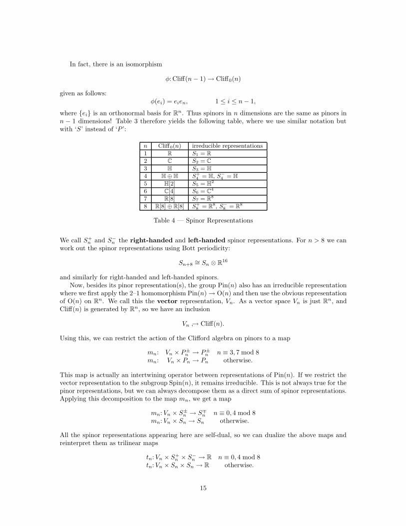
where {ei} is an orthonormal basis for Rn. Thus spinors in n dimensions are the same as pinors inn − 1 dimensions! Table 3 therefore yields the following table, where we use similar notation butwith ‘S’ instead of ‘P ’:

n Cliff0(n) irreducible representations

1 R S1 = R2 C S2 = C3 H S3 = H4 H⊕H S+

4 = H, S−4 = H5 H[2] S5 = H2

6 C[4] S6 = C4

7 R[8] S7 = R8

8 R[8] ⊕ R[8] S+8 = R8, S−8 = R8

Table 4 — Spinor Representations

We call S+n and S−n the right-handed and left-handed spinor representations. For n > 8 we can

work out the spinor representations using Bott periodicity:

Sn+8∼= Sn ⊗ R16

and similarly for right-handed and left-handed spinors.Now, besides its pinor representation(s), the group Pin(n) also has an irreducible representation

where we first apply the 2–1 homomorphism Pin(n)→ O(n) and then use the obvious representationof O(n) on Rn. We call this the vector representation, Vn. As a vector space Vn is just Rn, andCliff(n) is generated by Rn, so we have an inclusion

Vn ↪→ Cliff(n).

Using this, we can restrict the action of the Clifford algebra on pinors to a map

mn: Vn × P±n → P±n n ≡ 3, 7 mod 8mn: Vn × Pn → Pn otherwise.

This map is actually an intertwining operator between representations of Pin(n). If we restrict thevector representation to the subgroup Spin(n), it remains irreducible. This is not always true for thepinor representations, but we can always decompose them as a direct sum of spinor representations.Applying this decomposition to the map mn, we get a map

mn:Vn × S±n → S∓n n ≡ 0, 4 mod 8mn:Vn × Sn → Sn otherwise.

All the spinor representations appearing here are self-dual, so we can dualize the above maps andreinterpret them as trilinear maps

tn:Vn × S+n × S−n → R n ≡ 0, 4 mod 8

tn:Vn × Sn × Sn → R otherwise.

15

These trilinear maps are candidates for trialities! However, they can only be trialities when thedimension of the vector representation matches that of the relevant spinor representations. In therange of the above table this happens only for n = 1, 2, 4, 8. In these cases we actually do get normedtrialities, which in turn give normed division algebras:

t1:V1 × S1 × S1 → R gives R.t2:V2 × S2 × S2 → R gives C.t4:V4 × S+

4 × S−4 → R gives H.t8:V8 × S+

8 × S−8 → R gives O.

In higher dimensions, the spinor representations become bigger than the vector representation, sowe get no more trialities this way — and of course, none exist.

Of the four normed trialities, the one that gives the octonions has an interesting property thatthe rest lack. To see this property, one must pay careful attention to the difference between a normedtriality and a normed division algebra. To construct a normed division K algebra from the normedtriality t:V1 × V2 × V3 → R, we must arbitrarily choose unit vectors in two of the three spaces, sothe symmetry group of K is smaller than that of t. More precisely, let us define an automorphismof the normed triality t:V1 × V2 × V3 → R to be a triple of norm–preserving maps fi:Vi → Vi suchthat

t(f1(v1), f2(v2), f3(v3)) = t(v1, v2, v3)

for all vi ∈ Vi. These automorphisms form a group we call Aut(t). If we construct a normed divisionalgebra K from t by choosing unit vectors e1 ∈ V1, e2 ∈ V2, we have

Aut(K) ∼= {(f1, f2, f3) ∈ Aut(t) : f1(e1) = e1, f2(e2) = e2}.

In particular, it turns out that:

1 ∼= Aut(R) ⊆ Aut(t1) ∼= {(g1, g2, g3) ∈ O(1)3: g1g2g3 = 1}Z2

∼= Aut(C) ⊆ Aut(t2) ∼= {(g1, g2, g3) ∈ U(1)3: g1g2g3 = 1} × Z2

SO(3) ∼= Aut(H) ⊆ Aut(t4) ∼= Sp(1)3/{±(1, 1, 1)}G2

∼= Aut(O) ⊆ Aut(t8) ∼= Spin(8)

(5)

whereO(1) ∼= Z2, U(1) ∼= SO(2), Sp(1) ∼= SU(2)

are the unit spheres in R, C and H, respectively — the only spheres that are Lie groups. G2 is justanother name for the automorphism group of the octonions; we shall study this group in Section 4.1.The bigger group Spin(8) acts as automorphisms of the triality that gives the octonions, and it doesso in an interesting way. Given any element g ∈ Spin(8), there exist unique elements g± ∈ Spin(8)such that

t(g(v1), g+(v2), g−(v3)) = t(v1, v2, v3)

for all v1 ∈ V8, v2 ∈ S+8 , and v3 ∈ S−8 . Moreover, the maps

α±: g → g±

are outer automorphisms of Spin(8). In fact Out(Spin(8)) is the permutation group on 3 letters, andthere exist outer automorphisms that have the effect of permuting the vector, left-handed spinor,and right-handed spinor representations any way one likes; α+ and α− are among these.

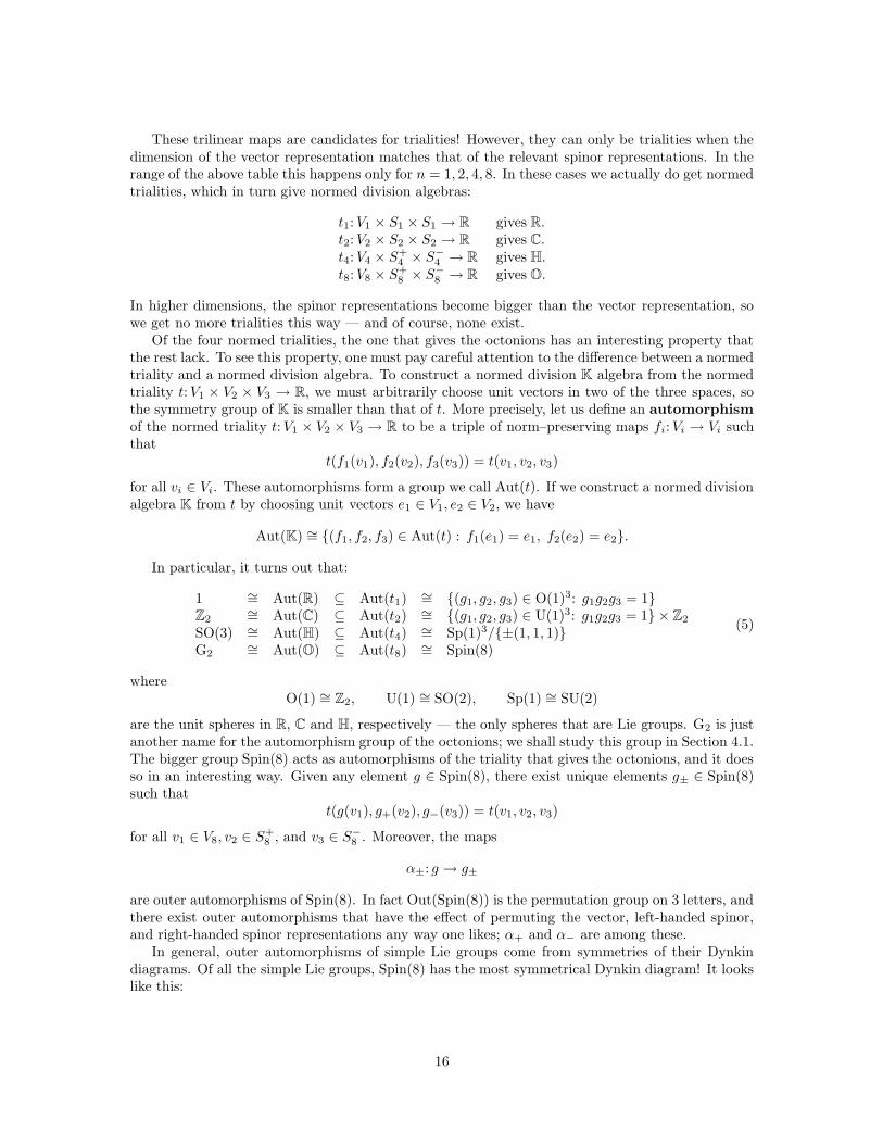
In general, outer automorphisms of simple Lie groups come from symmetries of their Dynkindiagrams. Of all the simple Lie groups, Spin(8) has the most symmetrical Dynkin diagram! It lookslike this:

16

Here the three outer nodes correspond to the vector, left-handed spinor and right-handed spinorrepresentations of Spin(8), while the central node corresponds to the adjoint representation —that is, the representation of Spin(8) on its own Lie algebra, better known as so(8). The outerautomorphisms corresponding to the symmetries of this diagram were discovered in 1925 by Cartan[17], who called these symmetries triality. The more general notion of ‘triality’ we have beendiscussing here came later, and is apparently due to Adams [2].

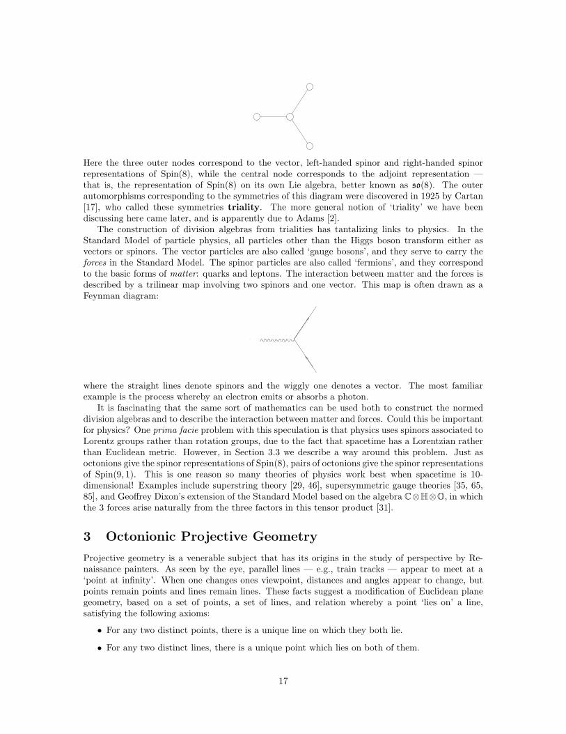
The construction of division algebras from trialities has tantalizing links to physics. In theStandard Model of particle physics, all particles other than the Higgs boson transform either asvectors or spinors. The vector particles are also called ‘gauge bosons’, and they serve to carry theforces in the Standard Model. The spinor particles are also called ‘fermions’, and they correspondto the basic forms of matter: quarks and leptons. The interaction between matter and the forces isdescribed by a trilinear map involving two spinors and one vector. This map is often drawn as aFeynman diagram:

where the straight lines denote spinors and the wiggly one denotes a vector. The most familiarexample is the process whereby an electron emits or absorbs a photon.

It is fascinating that the same sort of mathematics can be used both to construct the normeddivision algebras and to describe the interaction between matter and forces. Could this be importantfor physics? One prima facie problem with this speculation is that physics uses spinors associated toLorentz groups rather than rotation groups, due to the fact that spacetime has a Lorentzian ratherthan Euclidean metric. However, in Section 3.3 we describe a way around this problem. Just asoctonions give the spinor representations of Spin(8), pairs of octonions give the spinor representationsof Spin(9, 1). This is one reason so many theories of physics work best when spacetime is 10-dimensional! Examples include superstring theory [29, 46], supersymmetric gauge theories [35, 65,85], and Geoffrey Dixon’s extension of the Standard Model based on the algebra C⊗H⊗O, in whichthe 3 forces arise naturally from the three factors in this tensor product [31].

3 Octonionic Projective Geometry

Projective geometry is a venerable subject that has its origins in the study of perspective by Re-naissance painters. As seen by the eye, parallel lines — e.g., train tracks — appear to meet at a‘point at infinity’. When one changes ones viewpoint, distances and angles appear to change, butpoints remain points and lines remain lines. These facts suggest a modification of Euclidean planegeometry, based on a set of points, a set of lines, and relation whereby a point ‘lies on’ a line,satisfying the following axioms:

• For any two distinct points, there is a unique line on which they both lie.

• For any two distinct lines, there is a unique point which lies on both of them.

17

• There exist four points, no three of which lie on the same line.

• There exist four lines, no three of which have the same point lying on them.

A structure satisfying these axioms is called a projective plane. Part of the charm of this definitionis that it is ‘self-dual’: if we switch the words ‘point’ and ‘line’ and switch who lies on whom, itstays the same.

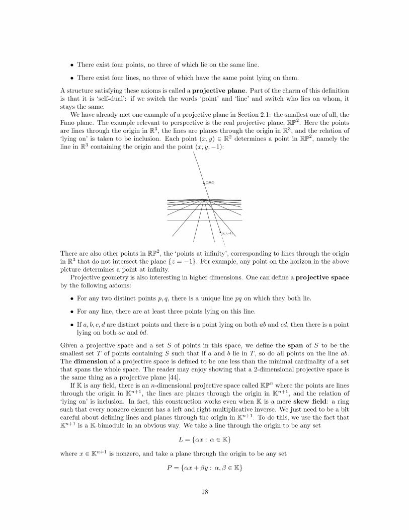
We have already met one example of a projective plane in Section 2.1: the smallest one of all, theFano plane. The example relevant to perspective is the real projective plane, RP2. Here the pointsare lines through the origin in R3, the lines are planes through the origin in R3, and the relation of‘lying on’ is taken to be inclusion. Each point (x, y) ∈ R2 determines a point in RP2, namely theline in R3 containing the origin and the point (x, y,−1):

(0,0,0)

( , ,−1)x y

There are also other points in RP2, the ‘points at infinity’, corresponding to lines through the originin R3 that do not intersect the plane {z = −1}. For example, any point on the horizon in the abovepicture determines a point at infinity.

Projective geometry is also interesting in higher dimensions. One can define a projective spaceby the following axioms:

• For any two distinct points p, q, there is a unique line pq on which they both lie.

• For any line, there are at least three points lying on this line.

• If a, b, c, d are distinct points and there is a point lying on both ab and cd, then there is a pointlying on both ac and bd.

Given a projective space and a set S of points in this space, we define the span of S to be thesmallest set T of points containing S such that if a and b lie in T , so do all points on the line ab.The dimension of a projective space is defined to be one less than the minimal cardinality of a setthat spans the whole space. The reader may enjoy showing that a 2-dimensional projective space isthe same thing as a projective plane [44].

If K is any field, there is an n-dimensional projective space called KPn where the points are linesthrough the origin in Kn+1, the lines are planes through the origin in Kn+1, and the relation of‘lying on’ is inclusion. In fact, this construction works even when K is a mere skew field: a ringsuch that every nonzero element has a left and right multiplicative inverse. We just need to be a bitcareful about defining lines and planes through the origin in Kn+1. To do this, we use the fact thatKn+1 is a K-bimodule in an obvious way. We take a line through the origin to be any set

L = {αx : α ∈ K}

where x ∈ Kn+1 is nonzero, and take a plane through the origin to be any set

P = {αx+ βy : α, β ∈ K}

18

where x, y ∈ Kn+1 are elements such that αx + βy = 0 implies α, β = 0.Given this example, the question naturally arises whether every projective n-space is of the form

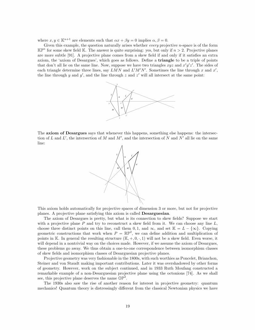
KPn for some skew field K. The answer is quite surprising: yes, but only if n > 2. Projective planesare more subtle [91]. A projective plane comes from a skew field if and only if it satisfies an extraaxiom, the ‘axiom of Desargues’, which goes as follows. Define a triangle to be a triple of pointsthat don’t all lie on the same line. Now, suppose we have two triangles xyz and x′y′z′. The sides ofeach triangle determine three lines, say LMN and L′M ′N ′. Sometimes the line through x and x′,the line through y and y′, and the line through z and z′ will all intersect at the same point:

x

y

M

L

N

y

zz

x

LN

M

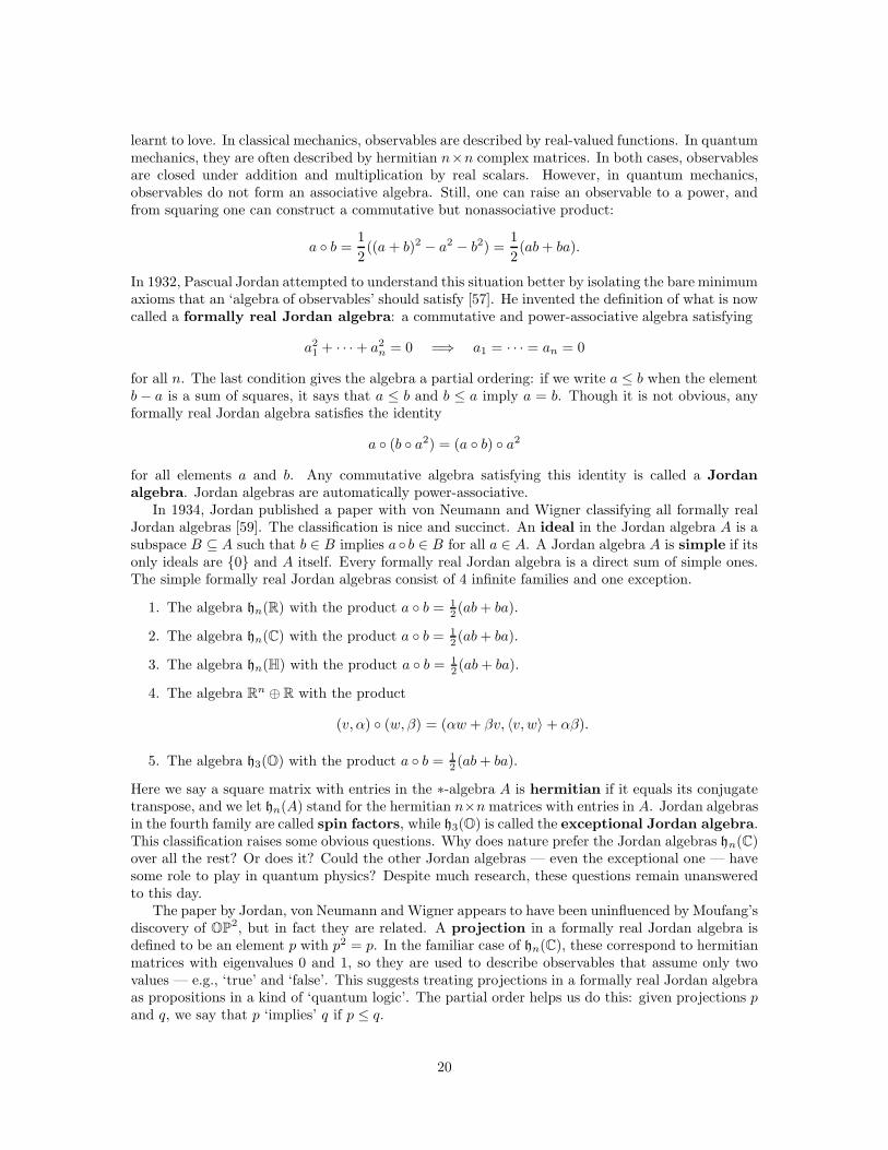
The axiom of Desargues says that whenever this happens, something else happens: the intersec-tion of L and L′, the intersection of M and M ′, and the intersection of N and N ′ all lie on the sameline:

N

M

LL

N

M

This axiom holds automatically for projective spaces of dimension 3 or more, but not for projectiveplanes. A projective plane satisfying this axiom is called Desarguesian.

The axiom of Desargues is pretty, but what is its connection to skew fields? Suppose we startwith a projective plane P and try to reconstruct a skew field from it. We can choose any line L,choose three distinct points on this line, call them 0, 1, and ∞, and set K = L − {∞}. Copyinggeometric constructions that work when P = RP2, we can define addition and multiplication ofpoints in K. In general the resulting structure (K,+, 0, ·, 1) will not be a skew field. Even worse, itwill depend in a nontrivial way on the choices made. However, if we assume the axiom of Desargues,these problems go away. We thus obtain a one-to-one correspondence between isomorphism classesof skew fields and isomorphism classes of Desarguesian projective planes.

Projective geometry was very fashionable in the 1800s, with such worthies as Poncelet, Brianchon,Steiner and von Staudt making important contributions. Later it was overshadowed by other formsof geometry. However, work on the subject continued, and in 1933 Ruth Moufang constructed aremarkable example of a non-Desarguesian projective plane using the octonions [74]. As we shallsee, this projective plane deserves the name OP2.

The 1930s also saw the rise of another reason for interest in projective geometry: quantummechanics! Quantum theory is distressingly different from the classical Newtonian physics we have

19

learnt to love. In classical mechanics, observables are described by real-valued functions. In quantummechanics, they are often described by hermitian n×n complex matrices. In both cases, observablesare closed under addition and multiplication by real scalars. However, in quantum mechanics,observables do not form an associative algebra. Still, one can raise an observable to a power, andfrom squaring one can construct a commutative but nonassociative product:

a ◦ b =1

2((a+ b)2 − a2 − b2) =

1

2(ab+ ba).

In 1932, Pascual Jordan attempted to understand this situation better by isolating the bare minimumaxioms that an ‘algebra of observables’ should satisfy [57]. He invented the definition of what is nowcalled a formally real Jordan algebra: a commutative and power-associative algebra satisfying

a21 + · · ·+ a2

n = 0 =⇒ a1 = · · · = an = 0

for all n. The last condition gives the algebra a partial ordering: if we write a ≤ b when the elementb− a is a sum of squares, it says that a ≤ b and b ≤ a imply a = b. Though it is not obvious, anyformally real Jordan algebra satisfies the identity

a ◦ (b ◦ a2) = (a ◦ b) ◦ a2

for all elements a and b. Any commutative algebra satisfying this identity is called a Jordanalgebra. Jordan algebras are automatically power-associative.

In 1934, Jordan published a paper with von Neumann and Wigner classifying all formally realJordan algebras [59]. The classification is nice and succinct. An ideal in the Jordan algebra A is asubspace B ⊆ A such that b ∈ B implies a ◦ b ∈ B for all a ∈ A. A Jordan algebra A is simple if itsonly ideals are {0} and A itself. Every formally real Jordan algebra is a direct sum of simple ones.The simple formally real Jordan algebras consist of 4 infinite families and one exception.

1. The algebra hn(R) with the product a ◦ b = 12 (ab+ ba).

2. The algebra hn(C) with the product a ◦ b = 12 (ab+ ba).

3. The algebra hn(H) with the product a ◦ b = 12 (ab+ ba).

4. The algebra Rn ⊕ R with the product

(v, α) ◦ (w, β) = (αw + βv, 〈v, w〉 + αβ).

5. The algebra h3(O) with the product a ◦ b = 12 (ab+ ba).

Here we say a square matrix with entries in the ∗-algebra A is hermitian if it equals its conjugatetranspose, and we let hn(A) stand for the hermitian n×n matrices with entries in A. Jordan algebrasin the fourth family are called spin factors, while h3(O) is called the exceptional Jordan algebra.This classification raises some obvious questions. Why does nature prefer the Jordan algebras hn(C)over all the rest? Or does it? Could the other Jordan algebras — even the exceptional one — havesome role to play in quantum physics? Despite much research, these questions remain unansweredto this day.

The paper by Jordan, von Neumann and Wigner appears to have been uninfluenced by Moufang’sdiscovery of OP2, but in fact they are related. A projection in a formally real Jordan algebra isdefined to be an element p with p2 = p. In the familiar case of hn(C), these correspond to hermitianmatrices with eigenvalues 0 and 1, so they are used to describe observables that assume only twovalues — e.g., ‘true’ and ‘false’. This suggests treating projections in a formally real Jordan algebraas propositions in a kind of ‘quantum logic’. The partial order helps us do this: given projections pand q, we say that p ‘implies’ q if p ≤ q.

20

The relation between Jordan algebras and quantum logic is already interesting [34], but thereal fun starts when we note that projections in hn(C) correspond to subspaces of Cn. This setsup a relationship to projective geometry [98], since the projections onto 1-dimensional subspacescorrespond to points in CPn, while the projections onto 2-dimensional subspaces correspond tolines. Even better, we can work out the dimension of a subspace V ⊆ Cn from the correspondingprojection p:Cn → V using only the partial order on projections: V has dimension d iff the longestchain of distinct projections

0 = p0 < · · · < pi = p

has length i = d. In fact, we can use this to define the rank of a projection in any formallyreal Jordan algebra. We can then try to construct a projective space whose points are the rank-1projections and whose lines are the rank-2 projections, with the relation of ‘lying on’ given by thepartial order ≤.

If we try this starting with hn(R), hn(C) or hn(H), we succeed when n ≥ 2, and we obtain theprojective spaces RPn, CPn and HPn, respectively. If we try this starting with the spin factor Rn⊕Rwe succeed when n ≥ 2, and obtain a series of 1-dimensional projective spaces related to Lorentziangeometry. Finally, in 1949 Jordan [58] discovered that if we try this construction starting with theexceptional Jordan algebra, we get the projective plane discovered by Moufang: OP2.

In what follows we describe the octonionic projective plane and exceptional Jordan algebra inmore detail. But first let us consider the octonionic projective line, and the Jordan algebra h2(O).

3.1 Projective Lines

A one-dimensional projective space is called a projective line. Projective lines are not very inter-esting from the viewpoint of axiomatic projective geometry, since they have only one line on whichall the points lie. Nonetheless, they can be geometrically and topologically interesting. This isespecially true of the octonionic projective line. As we shall see, this space has a deep connectionto Bott periodicity, and also to the Lorentzian geometry of 10-dimensional spacetime.

Suppose K is a normed division algebra. We have already defined KP1 when K is associative,but this definition does not work well for the octonions: it is wiser to take a detour through Jordanalgebras. Let h2(K) be the space of 2× 2 hermitian matrices with entries in K. It is easy to checkthat this becomes a Jordan algebra with the product a ◦ b = 1

2 (ab + ba). We can try to build aprojective space from this Jordan algebra using the construction in the previous section. To see ifthis succeeds, we need to ponder the projections in h2(K). A little calculation shows that besidesthe trivial projections 0 and 1, they are all of the form

(x∗

y∗

)(x y

)=

(x∗x x∗yy∗x y∗y

)

where (x, y) ∈ K2 has‖x‖2 + ‖y‖2 = 1.

These nontrivial projections all have rank 1, so they are the points of our would–be projective space.Our would–be projective space has just one line, corresponding to the projection 1, and all the pointslie on this line. It is easy to check that the axioms for a projective space hold. Since this projectivespace is 1-dimensional, we have succeeded in creating the projective line over K. We call the setof points of this projective line KP1.

Given any nonzero element (x, y) ∈ K2, we can normalize it and then use the above formula toget a point in KP1, which we call [(x, y)]. This allows us to describe KP1 in terms of lines throughthe origin, as follows. Define an equivalence relation on nonzero elements of K2 by

(x, y) ∼ (x′, y′) ⇐⇒ [(x, y)] = [(x′, y′)].

21

We call an equivalence class for this relation a line through the origin in K2. We can then identifypoints in KP1 with lines through the origin in K2.

Be careful: when K is the octonions, the line through the origin containing (x, y) is not alwaysequal to

{(αx, αy) : α ∈ K}.This is only true when K is associative, or when x or y is 1. Luckily, we have (x, y) ∼ (y−1x, 1)when y 6= 0 and (x, y) ∼ (1, x−1y) when x 6= 0. Thus in either case we get a concrete description ofthe line through the origin containing (x, y): when x 6= 0 it equals

{(α(y−1x), α) : α ∈ K},

and when y 6= 0 it equals{(α, α(x−1y) : α ∈ K}.

In particular, the line through the origin containing (x, y) is always a real vector space isomorphicto K.

We can make KP1 into a manifold as follows. By the above observations, we can cover it withtwo coordinate charts: one containing all points of the form [(x, 1)], the other containing all pointsof the form [(1, y)]. It is easy to check that [(x, 1)] = [(1, y)] iff y = x−1, so the transition functionfrom the first chart to the second is the map x 7→ x−1. Since this transition function and its inverseare smooth on the intersection of the two charts, KP1 becomes a smooth manifold.

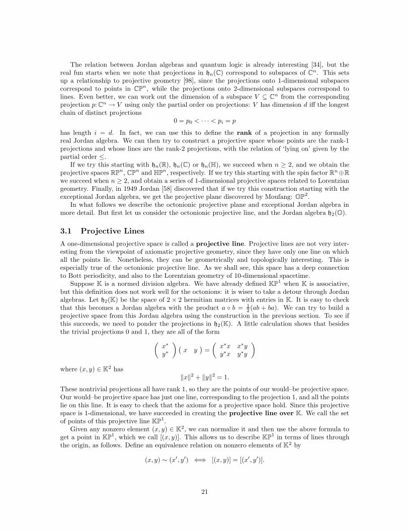
When pondering the geometry of projective lines it is handy to visualize the complex case, sinceCP1 is just the familiar ‘Riemann sphere’. In this case, the map

x 7→ [(x, 1)]

is given by stereographic projection:

x

[ ,1]x

0

where we choose the sphere to have diameter 1. This map from C to CP1 is one-to-one and almostonto, missing only the point at infinity, or ‘north pole’. Similarly, the map

y 7→ [(1, y)]

misses only the south pole. Composing the first map with the inverse of the second, we get themap x 7→ x−1, which goes by the name of ‘conformal inversion’. The southern hemisphere of theRiemann sphere consists of all points [(x, 1)] with ‖x‖ ≤ 1, while the northern hemisphere consistsof all [(1, y)] with ‖y‖ ≤ 1. Unit complex numbers x give points [(x, 1)] = [(1, x−1)] on the equator.

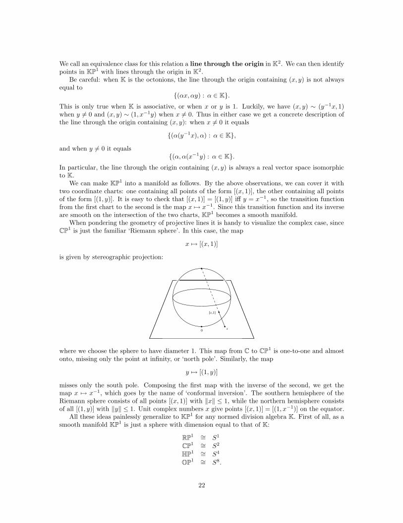
All these ideas painlessly generalize to KP1 for any normed division algebra K. First of all, as asmooth manifold KP1 is just a sphere with dimension equal to that of K:

RP1 ∼= S1

CP1 ∼= S2

HP1 ∼= S4

OP1 ∼= S8.

22

We can think of it as the one-point compactification of K. The ‘southern hemisphere’, ‘northernhemisphere’, and ‘equator’ of K have descriptions exactly like those given above for the complexcase. Also, as in the complex case, the maps x 7→ [(x, 1)] and y 7→ [(1, y)] are angle-preserving withrespect to the usual Euclidean metric on K and the round metric on the sphere.

One of the nice things about KP1 is that it comes equipped with a vector bundle whose fiber overthe point [(x, y)] is the line through the origin corresponding to this point. This bundle is called thecanonical line bundle, LK. Of course, when we are working with a particular division algebra,‘line’ means a copy of this division algebra, so if we think of them as real vector bundles, LR, LC, LHand LO have dimensions 1,2,4, and 8, respectively.

These bundles play an important role in topology, so it is good to understand them in a numberof ways. In general, any k-dimensional real vector bundle over Sn can be formed by taking trivialbundles over the northern and southern hemispheres and gluing them together along the equator viaa map f :Sn−1 → O(k). We must therefore be able to build the canonical line bundles LR, LC, LHand LO using maps

fR: S0 → O(1)fC: S1 → O(2)fH: S3 → O(4)fO: S7 → O(8).

What are these maps? We can describe them all simultaneously. Suppose K is a normed divisionalgebra of dimension n. In the southern hemisphere of KP1, we can identify any fiber of LK with Kby mapping the point (αx, α) in the line [(x, 1)] to the element α ∈ K. This trivializes the canonicalline bundle over the southern hemisphere. Similarly, we can trivialize this bundle over the northernhemisphere by mapping the point (β, βy) in the line [(1, y)] to the element β ∈ K. If x ∈ K hasnorm one, [(x, 1)] = [(1, x−1)] is a point on the equator, so we get two trivializations of the fiberover this point. These are related as follows: if (αx, α) = (β, βx−1) then β = αx. The map α 7→ βis thus right multiplication by x. In short,

fK:Sn−1 → O(n)

is just the map sending any norm-one element x ∈ K to the operation of right multiplication by x.The importance of the map fK becomes clearest if we form the inductive limit of the groups O(n)

using the obvious inclusions O(n) ↪→ O(n + 1), obtaining a topological group called O(∞). SinceO(n) is included in O(∞), we can think of fK as a map from Sn−1 to O(∞). Its homotopy class[fK] has the following marvelous property, mentioned in the Introduction:

• [fR] generates π0(O(∞)) ∼= Z2.

• [fC] generates π1(O(∞)) ∼= Z.

• [fH] generates π3(O(∞)) ∼= Z.

• [fO] generates π7(O(∞)) ∼= Z.

Another nice perspective on the canonical line bundles LK comes from looking at their unitsphere bundles. Any fiber of LK is naturally an inner product space, since it is a line through theorigin in K2. If we take the unit sphere in each fiber, we get a bundle of (n − 1)-spheres over KP1

called the Hopf bundle:pK:EK → KP1

The projection pK is called the Hopf map. The total space EK consists of all the unit vectors in

23

K2, so it is a sphere of dimension 2n− 1. In short, the Hopf bundles look like this:

K = R : S0 ↪→ S1 → S1

K = C : S1 ↪→ S3 → S2

K = H : S3 ↪→ S7 → S4

K = O : S7 ↪→ S15 → S8

We can understand the Hopf maps better by thinking about inverse images of points. The inverseimage p−1

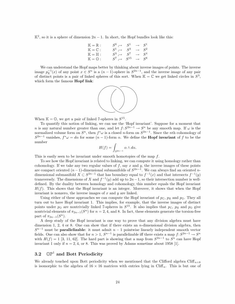
K (x) of any point x ∈ Sn is a (n − 1)-sphere in S2n−1, and the inverse image of any pairof distinct points is a pair of linked spheres of this sort. When K = C we get linked circles in S3,which form the famous Hopf link:

When K = O, we get a pair of linked 7-spheres in S15.To quantify this notion of linking, we can use the ‘Hopf invariant’. Suppose for a moment that

n is any natural number greater than one, and let f :S2n−1 → Sn be any smooth map. If ω is thenormalized volume form on Sn, then f∗ω is a closed n-form on S2n−1. Since the nth cohomology ofS2n−1 vanishes, f∗ω = dα for some (n − 1)-form α. We define the Hopf invariant of f to be thenumber

H(f) =

∫

S2n−1

α ∧ dα.

This is easily seen to be invariant under smooth homotopies of the map f .To see how the Hopf invariant is related to linking, we can compute it using homology rather than

cohomology. If we take any two regular values of f , say x and y, the inverse images of these pointsare compact oriented (n−1)-dimensional submanifolds of S2n−1. We can always find an oriented n-dimensional submanifold X ⊂ S2n−1 that has boundary equal to f−1(x) and that intersects f−1(y)transversely. The dimensions of X and f−1(y) add up to 2n−1, so their intersection number is well-defined. By the duality between homology and cohomology, this number equals the Hopf invariantH(f). This shows that the Hopf invariant is an integer. Moreover, it shows that when the Hopfinvariant is nonzero, the inverse images of x and y are linked.

Using either of these approaches we can compute the Hopf invariant of pC, pH and pO. They allturn out to have Hopf invariant 1. This implies, for example, that the inverse images of distinctpoints under pO are nontrivially linked 7-spheres in S15. It also implies that pC, pH and pO givenontrivial elements of π2n−1(Sn) for n = 2, 4, and 8. In fact, these elements generate the torsion-freepart of π2n−1(Sn).

A deep study of the Hopf invariant is one way to prove that any division algebra must havedimension 1, 2, 4 or 8. One can show that if there exists an n-dimensional division algebra, thenSn−1 must be parallelizable: it must admit n − 1 pointwise linearly independent smooth vectorfields. One can also show that for n > 1, Sn−1 is parallelizable iff there exists a map f :S2n−1 → Sn

with H(f) = 1 [3, 11, 62]. The hard part is showing that a map from S2n−1 to Sn can have Hopfinvariant 1 only if n = 2, 4, or 8. This was proved by Adams sometime about 1958 [1].

3.2 OP1 and Bott Periodicity

We already touched upon Bott periodicity when we mentioned that the Clifford algebra Cliffn+8

is isomorphic to the algebra of 16 × 16 matrices with entries lying in Cliffn. This is but one of

24

many related ‘period-8’ phenomena that go by the name of Bott periodicity. The appearance ofthe number 8 here is no coincidence: all these phenomena are related to the octonions! Since thismarvelous fact is somewhat under-appreciated, it seems worthwhile to say a bit about it. Here weshall focus on those aspects that are related to OP1 and the canonical octonionic line bundle overthis space.

Let us start with K-theory. This is a way of gaining information about a topological space bystudying the vector bundles over it. If the space has holes in it, there will be nontrivial vectorbundles that have ‘twists’ as we go around these holes. The simplest example is the ‘Mobius strip’bundle over S1, a 1-dimensional real vector bundle which has a 180◦ twist as we go around the circle.In fact, this is just the canonical line bundle LR. The canonical line bundles LC, LH and LO providehigher-dimensional analogues of this example.

K-theory tells us to study the vector bundles over a topological space X by constructing anabelian group as follows. First, take the set consisting of all isomorphism classes of real vectorbundles over X . Our ability to take direct sums of vector bundles gives this set an ‘addition’operation making it into a commutative monoid. Next, adjoin formal ‘additive inverses’ for all theelements of this set, obtaining an abelian group. This group is called KO(X), the real K-theoryof X . Alternatively we could start with complex vector bundles and get a group called K(X), buthere we will be interested in real vector bundles.

Any real vector bundle E over X gives an element [E] ∈ KO(X), and these elements generatethis group. If we pick a point in X , there is an obvious homomorphism dim:KO(X) → Z sending[E] to the dimension of the fiber of E at this point. Since the dimension is a rather obvious andboring invariant of vector bundles, it is nice to work with the kernel of this homomorphism, which iscalled the reduced real K-theory of X and denoted KO(X). This is an invariant of pointed spaces,i.e. spaces equipped with a designated point or basepoint.

Any sphere becomes a pointed space if we take the north pole as basepoint. The reduced realK-theory of the first eight spheres looks like this:

KO(S1) ∼= Z2

KO(S2) ∼= Z2

KO(S3) ∼= 0

KO(S4) ∼= ZKO(S5) ∼= 0

KO(S6) ∼= 0

KO(S7) ∼= 0

KO(S8) ∼= Z

where, as one might guess,

• [LR] generates KO(S1).

• [LC] generates KO(S2).

• [LH] generates KO(S4).

• [LO] generates KO(S8).

As mentioned in the previous section, one can build any k-dimensional real vector bundle overSn using a map f :Sn−1 → O(k). In fact, isomorphism classes of such bundles are in one-to-onecorrespondence with homotopy classes of such maps. Moreover, two such bundles determine thesame element of KO(X) if and only if the corresponding maps become homotopy equivalent after

25

we compose them with the inclusion O(k) ↪→ O(∞), where O(∞) is the direct limit of the groupsO(k). It follows that

KO(Sn) ∼= πn−1(O(∞)).

This fact gives us the list of homotopy groups of O(∞) which appears in the Introduction. It alsomeans that to prove Bott periodicity for these homotopy groups:

πi+8(O(∞)) ∼= πi(O(∞)),

it suffices to prove Bott periodicity for real K-theory:

KO(Sn+8) ∼= KO(Sn).

Why do we have Bott periodicity in real K-theory? It turns out that there is a graded ring KOwith

KOn = KO(Sn).

The product in this ring comes from our ability to take ‘smash products’ of spheres and also of realvector bundles over these spheres. Multiplying by [LO] gives an isomorphism

KO(Sn) → KO(Sn+8)x 7→ [LO]x

In other words, the canonical octonionic line bundle over OP1 generates Bott periodicity!There is much more to say about this fact and how it relates to Bott periodicity for Clifford

algebras, but alas, this would take us too far afield. We recommend that the interested reader turnto some introductory texts on K-theory, for example the one by Dale Husemoller [56]. Unfortunately,all the books I know downplay the role of the octonions. To spot it, one must bear in mind therelation between the octonions and Clifford algebras, discussed in Section 2.3 above.

3.3 OP1 and Lorentzian Geometry

In Section 3.1 we sketched a systematic approach to projective lines over the normed division alge-bras. The most famous example is the Riemann sphere, CP1. As emphasized by Penrose [77], thisspace has a fascinating connection to Lorentzian geometry — or in other words, special relativity.All conformal transformations of the Riemann sphere come from fractional linear transformations

z 7→ az + b

cz + d, a, b, c, d ∈ C.

It is easy to see that the group of such transformations is isomorphic to PSL(2,C): 2× 2 complexmatrices with determinant 1, modulo scalar multiples of the identity. Less obviously, it is also isomor-phic to the Lorentz group SO0(3, 1): the identity component of the group of linear transformationsof R4 that preserve the Minkowski metric

x · y = x1y1 + x2y2 + x3y3 − x4y4.

This fact has a nice explanation in terms of the ‘heavenly sphere’. Mathematically, this is the 2-sphere consisting of all lines of the form {αx} where x ∈ R4 has x · x = 0. In special relativity suchlines represent light rays, so the heavenly sphere is the sphere on which the stars appear to lie whenyou look at the night sky. This sphere inherits a conformal structure from the Minkowski metric onR4. This allows us to identify the heavenly sphere with CP1, and it implies that the Lorentz groupacts as conformal transformations of CP1. In concrete terms, what this means is that if you shootpast the earth at nearly the speed of light, the constellations in the sky will appear distorted, butall angles will be preserved.

26

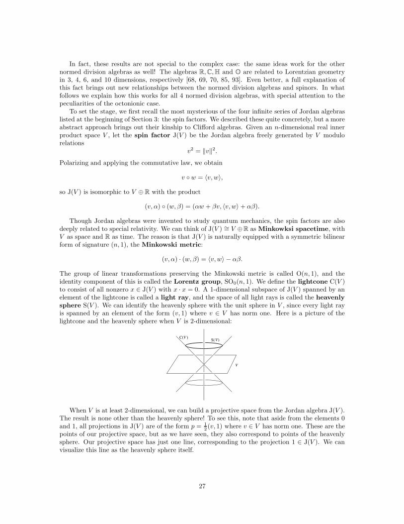
In fact, these results are not special to the complex case: the same ideas work for the othernormed division algebras as well! The algebras R,C,H and O are related to Lorentzian geometryin 3, 4, 6, and 10 dimensions, respectively [68, 69, 70, 85, 93]. Even better, a full explanation ofthis fact brings out new relationships between the normed division algebras and spinors. In whatfollows we explain how this works for all 4 normed division algebras, with special attention to thepeculiarities of the octonionic case.

To set the stage, we first recall the most mysterious of the four infinite series of Jordan algebraslisted at the beginning of Section 3: the spin factors. We described these quite concretely, but a moreabstract approach brings out their kinship to Clifford algebras. Given an n-dimensional real innerproduct space V , let the spin factor J(V ) be the Jordan algebra freely generated by V modulorelations

v2 = ‖v‖2.Polarizing and applying the commutative law, we obtain

v ◦ w = 〈v, w〉,

so J(V ) is isomorphic to V ⊕ R with the product

(v, α) ◦ (w, β) = (αw + βv, 〈v, w〉 + αβ).

Though Jordan algebras were invented to study quantum mechanics, the spin factors are alsodeeply related to special relativity. We can think of J(V ) ∼= V ⊕R as Minkowksi spacetime, withV as space and R as time. The reason is that J(V ) is naturally equipped with a symmetric bilinearform of signature (n, 1), the Minkowski metric:

(v, α) · (w, β) = 〈v, w〉 − αβ.

The group of linear transformations preserving the Minkowski metric is called O(n, 1), and theidentity component of this is called the Lorentz group, SO0(n, 1). We define the lightcone C(V )to consist of all nonzero x ∈ J(V ) with x · x = 0. A 1-dimensional subspace of J(V ) spanned by anelement of the lightcone is called a light ray, and the space of all light rays is called the heavenlysphere S(V ). We can identify the heavenly sphere with the unit sphere in V , since every light rayis spanned by an element of the form (v, 1) where v ∈ V has norm one. Here is a picture of thelightcone and the heavenly sphere when V is 2-dimensional:

VC( )VS( )

V

When V is at least 2-dimensional, we can build a projective space from the Jordan algebra J(V ).The result is none other than the heavenly sphere! To see this, note that aside from the elements 0and 1, all projections in J(V ) are of the form p = 1

2 (v, 1) where v ∈ V has norm one. These are thepoints of our projective space, but as we have seen, they also correspond to points of the heavenlysphere. Our projective space has just one line, corresponding to the projection 1 ∈ J(V ). We canvisualize this line as the heavenly sphere itself.

27

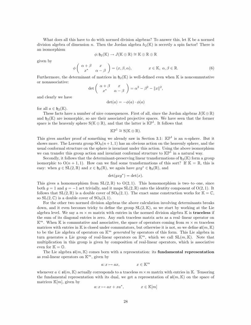
What does all this have to do with normed division algebras? To answer this, let K be a normeddivision algebra of dimension n. Then the Jordan algebra h2(K) is secretly a spin factor! There isan isomorphism

φ: h2(K)→ J(K⊕ R) ∼= K⊕ R⊕ Rgiven by

φ

(α+ β xx∗ α− β

)= (x, β, α), x ∈ K, α, β ∈ R. (6)

Furthermore, the determinant of matrices in h2(K) is well-defined even when K is noncommutativeor nonassociative:

det

(α+ β xx∗ α− β

)= α2 − β2 − ‖x‖2,

and clearly we havedet(a) = −φ(a) · φ(a)

for all a ∈ h2(K).These facts have a number of nice consequences. First of all, since the Jordan algebras J(K⊕R)

and h2(K) are isomorphic, so are their associated projective spaces. We have seen that the formerspace is the heavenly sphere S(K⊕ R), and that the latter is KP1. It follows that

KP1 ∼= S(K⊕ R).

This gives another proof of something we already saw in Section 3.1: KP1 is an n-sphere. But itshows more. The Lorentz group SO0(n+1, 1) has an obvious action on the heavenly sphere, and theusual conformal structure on the sphere is invariant under this action. Using the above isomorphismwe can transfer this group action and invariant conformal structure to KP1 in a natural way.

Secondly, it follows that the determinant-preserving linear transformations of h2(K) form a groupisomorphic to O(n + 1, 1). How can we find some transformations of this sort? If K = R, this iseasy: when g ∈ SL(2,R) and x ∈ h2(R), we again have gxg∗ ∈ h2(R), and

det(gxg∗) = det(x).

This gives a homomorphism from SL(2,R) to O(2, 1). This homomorphism is two–to–one, sinceboth g = 1 and g = −1 act trivially, and it maps SL(2,R) onto the identity component of O(2, 1). Itfollows that SL(2,R) is a double cover of SO0(2, 1). The exact same construction works for K = C,so SL(2,C) is a double cover of SO0(3, 1).

For the other two normed division algebras the above calculation involving determinants breaksdown, and it even becomes tricky to define the group SL(2,K), so we start by working at the Liealgebra level. We say a m×m matrix with entries in the normed division algebra K is traceless ifthe sum of its diagonal entries is zero. Any such traceless matrix acts as a real–linear operator onKm. When K is commutative and associative, the space of operators coming from m×m tracelessmatrices with entries in K is closed under commutators, but otherwise it is not, so we define sl(m,K)to be the Lie algebra of operators on Km generated by operators of this form. This Lie algebra inturn generates a Lie group of real-linear operators on Km, which we call SL(m,K). Note thatmultiplication in this group is given by composition of real-linear operators, which is associativeeven for K = O.

The Lie algebra sl(m,K) comes born with a representation: its fundamental representationas real-linear operators on Km, given by

a:x 7→ ax, x ∈ Km

whenever a ∈ sl(m,K) actually corresponds to a traceless m×m matrix with entries in K. Tensoringthe fundamental representation with its dual, we get a representation of sl(m,K) on the space ofmatrices K[m], given by

a:x 7→ ax+ xa∗, x ∈ K[m]

28

whenever a is a traceless matrix with entries in K. Since ax + xa∗ is hermitian whenever x is, thisrepresentation restricts to a representation of sl(m,K) on hm(K). This in turn can be exponentiatedto obtain a representation of the group SL(m,K) on hm(K).

Now let us return to the case m = 2. One can prove that the representation of SL(2,K) on h2(K)is determinant-preserving simply by checking that

d

dtdet(x + t(ax+ xa∗))

∣∣∣t=0

= 0

when x lies in h2(K) and a ∈ K[2] is traceless. Here the crucial thing is to make sure that thecalculation is not spoiled by noncommutativity or nonassociativity. It follows that we have a homo-morphism

αK: SL(2,K)→ SO0(n+ 1, 1)

One can check that this is onto, and that its kernel consists of the matrices ±1. Thus if we define

PSL(2,K) = SL(2,K)/{±1},

we get isomorphismsPSL(2,R) ∼= SO0(2, 1)PSL(2,C) ∼= SO0(3, 1)PSL(2,H) ∼= SO0(6, 1)PSL(2,O) ∼= SO0(9, 1).

Putting this together with our earlier observations, it follows that PSL(2,K) acts as conformaltransformations of KP1.

We conclude with some words about how all this relates to spinors. The machinery of Cliffordalgebras and spinors extends effortlessly from the case of inner product spaces to vector spacesequipped with an indefinite metric. In particular, the Lorentz group SO0(n + 1, 1) has a doublecover called Spin(n+ 1, 1), and this group has certain representations called spinor representations.When n = 1, 2, 4 or 8, we actually have

Spin(n+ 1, 1) ∼= SL(2,K)

where K is the normed division algebra of dimension n. The fundamental representation of SL(2,K)on K2 is the left-handed spinor representation of Spin(n+ 1, 1). Its dual is the right-handed spinorrepresentation. Moreover, the interaction between vectors and spinors that serves as the basis ofsupersymmetric theories of physics in spacetimes of dimension 3, 4, 6 and 10 is just the action ofh2(K) on K2 by matrix multiplication. In a Feynman diagram, this is represented as follows:

K2

h2(K)

K2

In the case K = C, Penrose [77] has described a nice trick for getting points on the heavenlysphere from spinors. In fact, it also works for other normed division algebras: if (x, y) ∈ K2 isnonzero, the hermitian matrix

(xy

)(x∗ y∗

)=

(xx∗ xy∗

yx∗ yy∗

)

29

is nonzero but has determinant zero, so it defines a point on the heavenly sphere. If we restrict tospinors of norm one, this trick reduces to the Hopf map. Moreover, it clarifies the curious double roleof KP1 as both the heavenly sphere in special relativity and a space of propositions in the quantumlogic associated to the Jordan algebra h2(K): any point on the heavenly sphere corresponds to aproposition specifying the state of a spinor!

3.4 OP2 and the Exceptional Jordan Algebra

The octonions are fascinating in themselves, but the magic really starts when we use them toconstruct the exceptional Jordan algebra h3(O) and its associated projective space, the octonionicprojective plane. The symmetry groups of these structures turn out to be exceptional Lie groups, andtriality gains an eerie pervasive influence over the proceedings, since an element of h3(O) consists of3 octonions and 3 real numbers. Using the relation between normed division algebras and trialities,we get an isomorphism

h3(O) ∼= R3 ⊕ V8 ⊕ S+8 ⊕ S−8

α z y∗

z∗ β xy x∗ γ

7→ ((α, β, γ), x, y, z)

(7)

where α, β, γ ∈ R and x, y, z ∈ O. Examining the Jordan product in h3(O) then reveals a wonderfulfact: while superficially this product is defined using the ∗-algebra structure of O, it can actually bedefined using only the natural maps

V8 × S+8 → S−8 , V8 × S−8 → S+

8 , S+8 × S−8 → V8

together with the inner products on these 3 spaces. All this information is contained in the normedtriality

t8:V8 × S+8 × S−8 → R,

so any automorphism of this triality gives a automorphism of h3(O). In Section 2.4 we saw thatAut(t8) ∼= Spin(8). With a little thought, it follows that

Spin(8) ⊆ Aut(h3(O)).

However, this picture of h3(O) in terms of 8-dimensional Euclidean geometry is just part of abigger picture — a picture set in 10-dimensional Minkowski spacetime! If we regard h2(O) as sittingin the lower right-hand corner of h3(O), we get an isomorphism

h3(O) ∼= R⊕ h2(O)⊕O2

(α ψ∗

ψ a

)7→ (α, a, ψ)

(8)

We saw in Section 3.3 that a ∈ h2(O) and ψ ∈ O2 can be identified with a vector and a spinor in10-dimensional Minkowski spacetime, respectively. Similarly, α is a scalar.

This picture gives a representation of Spin(9, 1) as linear transformations of h3(O). Unfortunately,most of these transformations do not preserve the Jordan product on h3(O). As we shall see, theyonly preserve a lesser structure on h3(O): the determinant. However, the transformations comingfrom the subgroup Spin(9) ⊂ Spin(9, 1) do preserve the Jordan product. We can see this as follows.As a representation of Spin(9), h2(O) splits into ‘space’ and ‘time’:

h2(O) ∼= V9 ⊕ R

30

with the two pieces corresponding to the traceless elements of h2(O) and the real multiples of theidentity, respectively. On the other hand, the spinor representation of so(9) splits as S+

8 ⊕S−8 whenwe restrict it to so(8), so we have

O2 ∼= S9.

We thus obtain an isomorphism

h3(O) ∼= R2 ⊕ V9 ⊕ S9

(α ψ∗

ψ a+ β

)7→ ((α, β), a, ψ)

(9)

where a ∈ h2(O) has vanishing trace and β is a real multiple of the identity. In these terms, one caneasily check that the Jordan product in h3(O) is built from invariant operations on scalars, vectorsand spinors in 9 dimensions. It follows that

Spin(9) ⊆ Aut(h3(O)).

For more details on this, see Harvey’s book [54].This does not exhaust all the symmetries of h3(O), since there are other automorphisms coming

from the permutation group on 3 letters, which acts on (α, β, γ) ∈ R3 and (x, y, z) ∈ O3 in anobvious way. Also, any matrix g ∈ O(3) acts by conjugation as an automorphism of h3(O); sincethe entries of g are real, there is no problem with nonassociativity here. The group Spin(9) is 36-dimensional, but the full automorphism group h3(O) is much bigger: it is 52-dimensional. As weexplain in Section 4.2, it goes by the name of F4.

However, we can already do something interesting with the automorphisms we have: we can usethem to diagonalize any element of h3(O). To see this, first note that the rotation group, and thusSpin(9), acts transitively on the unit sphere in V9. This means we can use an automorphism in ourSpin(9) subgroup to bring any element of h3(O) to the form

α z y∗

z∗ β xy x∗ γ

where x is real. The next step is to apply an automorphism that makes y and z real while leaving xalone. To do this, note that the subgroup of Spin(9) fixing any nonzero vector in V9 is isomorphicto Spin(8). When we restrict the representation S9 to this subgroup, it splits as S+

8 ⊕S−8 , and withsome work [54] one can show that Spin(8) acts on S+

8 ⊕ S−8 ∼= O2 in such a way that any element(y, z) ∈ O2 can be carried to an element with both components real. The final step is to take ourelement of h3(O) with all real entries and use an automorphism to diagonalize it. We can do this byconjugating it with a suitable matrix in O(3).

To understand OP2, we need to understand projections in h3(O). Here is where our abilityto diagonalize matrices in h3(O) via automorphisms comes in handy. Up to automorphism, everyprojection in h3(O) looks like one of these four:

p0 =

0 0 00 0 00 0 0

, p1 =

1 0 00 0 00 0 0

, p2 =

1 0 00 1 00 0 0

, p3 =

1 0 00 1 00 0 1

.

Now, the trace of a matrix in h3(O) is invariant under automorphisms, because we can define itusing only the Jordan algebra structure:

tr(a) =1

9tr(La), a ∈ h3(O)

31

where La is left multiplication by a. It follows that the trace of any projection in h3(O) is 0,1,2, or3. Furthermore, the rank of any projection p ∈ h3(O) equals its trace. To see this, first note thattr(p) ≥ rank(p), since p < q implies tr(p) < tr(q), and the trace goes up by integer steps. Thus weonly need show tr(p) ≤ rank(p). For this it suffices to consider the four projections shown above, asboth trace and rank are invariant under automorphisms. Since p0 < p1 < p2 < p3, it is clear thatfor these projections we indeed have tr(p) ≤ rank(p).

It follows that the points of the octonionic projective plane are projections with trace 1 in h3(O),while the lines are projections with trace 2. A calculation [54] shows that any projection with trace1 has the form

p =

xyz

( x∗ y∗ z∗

)=

xx∗ xy∗ xz∗

yx∗ yy∗ yz∗

zx∗ zy∗ zz∗

(10)

where (x, y, z) ∈ O3 has

(xy)z = x(yz), ‖x‖2 + ‖y‖2 + ‖z‖2 = 1.

On the other hand, any projection with trace 2 is of the form 1− p where p has trace 1. This setsup a one-to-one correspondence between points and lines in the octonionic projective plane. If weuse this correspondence to think of both as trace-1 projections, the point p lies on the line p′ ifand only if p < 1 − p′. Of course, p < 1 − p′ iff p′ < 1 − p. The symmetry of this relation meansthe octonionic projective plane is self-dual! This is also true of the real, complex and quaternionicprojective planes. In all cases, the operation that switches points and lines corresponds in quantumlogic to the ‘negation’ of propositions [98].

We use OP2 to stand for the set of points in the octonionic projective plane. Given any nonzeroelement (x, y, z) ∈ O3 with (xy)z = x(yz), we can normalize it and then use equation (10) to obtaina point [(x, y, z)] ∈ OP2. Copying the strategy that worked for OP1, we can make OP2 into a smoothmanifold by covering it with three coordinate charts:

• one chart containing all points of the form [(x, y, 1)],

• one chart containing all points of the form [(x, 1, z)],

• one chart containing all points of the form [(1, y, z)].

Checking that this works is a simple calculation. The only interesting part is to make sure thatwhenever the associative law might appear necessary, we can either use the alternativity of theoctonions or the fact that only triples with (xy)z = x(yz) give points [(x, y, z)] ∈ OP2.

We thus obtain the following picture of the octonionic projective plane. As a manifold, OP2 is16-dimensional. The lines in OP2 are copies of OP1, and thus 8-spheres. For any two distinct pointsin OP2, there is a unique line on which they both lie. For any two distinct lines, there is a uniquepoint lying on both of them. There is a ‘duality’ transformation that maps points to lines and viceversa while preserving this incidence relation. In particular, since the space of all points lying onany given line is a copy of OP1, so is the space of all lines containing a given point!

To dig more deeply into the geometry of OP2 one needs another important structure on theexceptional Jordan algebra: the determinant. We saw in Section 3.3 that despite noncommutativityand nonassociativity, the determinant of a matrix in h2(O) is a well-defined and useful concept. Thesame holds for h3(O)! We can define the determinant of a matrix in h3(O) by

det

α z y∗

z∗ β xy x∗ γ

= αβγ − (α‖x‖2 + β‖y‖2 + γ‖z‖2) + 2Re(xyz).

We can express this in terms of the trace and product via

det(a) =1

3tr(a3)− 1

2tr(a2)tr(a) +

1

6tr(a)

3.

32

This shows that the determinant is invariant under all automorphisms of h3(O). However, thedeterminant is invariant under an even bigger group of linear transformations. As we shall see inSection 4.4, this group is 78-dimensional: it is a noncompact real form of the exceptional Lie groupE6. This extra symmetry makes it worth seeing how much geometry we can do starting with justthe determinant and the vector space structure of h3(O).

The determinant is a cubic form on h3(O), so there is a unique symmetric trilinear form

(·, ·, ·): h3(O)× h3(O)× h3(O)→ R

such that(a, a, a) = det(a).

By dualizing this, we obtain the so-called cross product

×: h3(O)× h3(O)→ h3(O)∗.

Explicitly, this is given by(a× b)(c) = (a, b, c).

Despite its name, this product is commutative.We have already seen that points of OP2 correspond to trace-1 projections in h3(O). Freudenthal

[40] noticed that these are the same as elements p ∈ h3(O) with tr(p) = 1 and p × p = 0. Evenbetter, we can drop the equation tr(p) = 1 as long as we promise to work with equivalence classes ofnonzero elements satisfying p×p = 0, where two such elements are equivalent when one is a nonzeroreal multiple of the other. Each such equivalence class [p] corresponds to a unique point of OP2, andwe get all the points this way.

Given two points [p] and [q], their cross product p×q is well-defined up to a nonzero real multiple.This suggests that we define a ‘line’ to be an equivalence class of elements p×q ∈ h3(O)∗, where againtwo such elements are deemed equivalent if one is a nonzero real multiple of the other. Freudenthalshowed that we get a projective plane isomorphic to OP2 if we take these as our definitions of pointsand lines and decree that the point [p] lies on the line [L] if and only if L(p) = 0. Note that thisequation makes sense even though L and p are only well-defined up to nonzero real multiples.

One consequence of all this is that one can recover the structure of OP2 as a projective planestarting from just the determinant on h3(O): we did not need the Jordan algebra structure! However,to get a ‘duality’ map switching points and lines while preserving the incidence relation, we need abit more: we need the nondegenerate pairing

〈a, b〉 = tr(ab)

on h3(O). This sets up an isomorphism

h3(O) ∼= h3(O)∗.

This isomorphism turns out to map points to lines, and in fact, it sets up a one-to-one correspondencebetween points and lines. We can use this correspondence to think of both points and lines inOP2 as equivalence classes of elements of h3(O). In these terms, the point p lies on the line ` iff〈`, p〉 = 0. This relationship is symmetrical! It follows that if we switch points and lines using thiscorrespondence, the incidence relation is preserved.

We thus obtain a very pretty setup for working with OP2. If we use the isomorphism betweenh3(O) and its dual to reinterpret the cross product as a map

×: h3(O)× h3(O)→ h3(O),

then not only is the line through distinct points [p] and [q] given by [p × q], but also the point inwhich two distinct lines [`] and [m] meet is given by [` × m]. A triple of points [p], [q] and [r] is

33

collinear iff (p, q, r) = 0, and a triple of lines [`], [m], [n] meets at a point iff (`,m, n) = 0. Inaddition, there is a delightful bunch of identities relating the Jordan product, the determinant, thecross product and the inner product in h3(O).

For more on octonionic geometry, the reader is urged to consult the original papers by Freudenthal[39, 40, 41, 42], Jacques Tits [94, 95] and Tonny Springer [87, 88, 89]. The book by Helmut Salzmannet al is also good [82]. Unfortunately, we must now bid goodbye to this subject and begin our tripthrough the exceptional groups. However, we shall return to study the symmetries of OP2 and theexceptional Jordan algebra in Sections 4.2 and 4.4.

4 Exceptional Lie Algebras

On October 18th, 1887, Wilhelm Killing wrote a letter to Friedrich Engel saying that he had classifiedthe simple Lie algebras. In the next three years, this revolutionary work was published in a series ofpapers [63]. Besides what we now call the ‘classical’ simple Lie algebras, he claimed to have found6 ‘exceptional’ ones — new mathematical objects whose existence had never before been suspected.In fact he gave a rigorous construction of only the smallest of these. In his 1894 thesis, Cartan [14]constructed all of them and noticed that the two 52-dimensional exceptional Lie algebras discoveredby Killing were isomorphic, so that there are really only 5.

The Killing-Cartan classification of simple Lie algebras introduced much of the technology thatis now covered in any introductory course on the subject, such as roots and weights. In what followswe shall avoid this technology, since we wish instead to see the exceptional Lie algebras as octonionicrelatives of the classical ones — slightly eccentric relatives, but still having a close connection togeometry, in particular the Riemannian geometry of projective planes. It is also for this reason thatwe shall focus on the compact real forms of the simple Lie algebras.

The classical simple Lie algebras can be organized in three infinite families:

so(n) = {x ∈ R[n]: x∗ = −x, tr(x) = 0},su(n) = {x ∈ C[n]: x∗ = −x, tr(x) = 0},sp(n) = {x ∈ H[n]: x∗ = −x}.

The corresponding Lie groups are

SO(n) = {x ∈ R[n]: xx∗ = 1, det(x) = 1},SU(n) = {x ∈ C[n]: xx∗ = 1, det(x) = 1},Sp(n) = {x ∈ H[n]: xx∗ = 1}.

These arise naturally as symmetry groups of projective spaces over R, C, and H, respectively. Moreprecisely, they arise as groups of isometries: transformations that preserve a specified Riemannianmetric. Let us sketch how this works, as a warmup for the exceptional groups.

First consider the projective space RPn. We can think of this as the unit sphere in Rn+1 withantipodal points x and −x identified. It thus inherits a Riemannian metric from the sphere, andthe obvious action of the rotation group O(n+ 1) as isometries of the sphere yields an action of thisgroup as isometries of RPn with this metric. In fact, with this metric, the group of all isometries ofRPn is just

Isom(RPn) ∼= O(n+ 1)/O(1)

where O(1) = {±1} is the subgroup of O(n+ 1) that acts trivially on RPn. The Lie algebra of thisisometry group is

isom(RPn) ∼= so(n+ 1).

The case of CPn is very similar. We can think of this as the unit sphere in Cn+1 with pointsx and αx identified whenever α is a unit complex number. It thus inherits a Riemannian metric

34

from this sphere, and the unitary group U(n + 1) acts as isometries. If we consider only the con-nected component of the isometry group and ignore the orientation-reversing isometries coming fromcomplex conjugation, we have

Isom0(CPn) ∼= U(n+ 1)/U(1)

where U(1) is the subgroup that acts trivially on CPn. The Lie algebra of this isometry group is

isom(CPn) ∼= su(n+ 1).

The case of HPn is subtler, since we must take the noncommutativity of the quaternions intoaccount. We can think of HPn as the unit sphere in Hn+1 with points x and αx identified wheneverα is a unit quaternion, and as before, HPn inherits a Riemannian metric. The group Sp(n+ 1) actsas isometries of HPn, but this action comes from right multiplication, so

Isom(HPn) ∼= Sp(n+ 1)/{±1},

since not Sp(1) but only its center {±1} acts trivially on HPn by right multiplication. At the Liealgebra level, this gives

isom(HPn) ∼= sp(n+ 1).

For lovers of the octonions, it is tempting to try a similar construction starting with OP2. Whilenonassociativity makes things a bit tricky, we show in Section 4.2 that it can in fact be done. Itturns out that Isom(OP2) is one of the exceptional Lie groups, namely F4. Similarly, the exceptionalLie groups E6, E7 and E8 are in a certain subtle sense the isometry groups of projective planes overthe algebras C ⊗ O, H ⊗ O and O ⊗ O. Together with F4, these groups can all be defined by theso-called ‘magic square’ construction, which makes use of much of the algebra we have described sofar. We explain three versions of this construction in Section 4.3. We then treat the groups E6,E7

and E8 individually in the following sections. But first, we must introduce G2: the smallest of theexceptional Lie groups, and none other than the automorphism group of the octonions.

4.1 G2

In 1914, Elie Cartan noted that the smallest of the exceptional Lie groups, G2, is the automorphismgroup of the octonions [15]. Its Lie algebra g2 is therefore der(O), the derivations of the octonions.Let us take these facts as definitions of G2 and its Lie algebra, and work out some of the consequences.

What are automorphisms of the octonions like? One way to analyze this involves subalgebras ofthe octonions. Any octonion e1 whose square is −1 generates a subalgebra of O isomorphic to C.If we then pick any octonion e2 with square equal to −1 that anticommutes with e1, the elementse1, e2 generate a subalgebra isomorphic to H. Finally, if we pick any octonion e3 with square equalto −1 that anticommutes with e1, e2, and e1e2, the elements e1, e2, e3 generate all of O. We callsuch a triple of octonions a basic triple. Given any basic triple, there exists a unique way to definee4, . . . , e7 so that the whole multiplication table in Section 2 holds. In fact, this follows from theremarks on the Cayley–Dickson construction at the end of Section 2.3.

It follows that given any two basic triples, there exists a unique automorphism of O mappingthe first to the second. Conversely, it is obvious that any automorphism maps basic triples to basictriples. This gives a nice description of the group G2, as follows.

Fix a basic triple e1, e2, e3. There is a unique automorphism of the octonions mapping this toany other basic triple, say e′1, e

′2, e′3. Now our description of basic triples so far has been purely

algebraic, but we can also view them more geometrically as follows: a basic triple is any triple ofunit imaginary octonions (i.e. imaginary octonions of norm one) such that each is orthogonal to thealgebra generated by the other two. This means that our automorphism can map e1 to any pointe′1 on the 6-sphere of unit imaginary octonions, then map e2 to any point e′2 on the 5-sphere of unit

35

imaginary octonions that are orthogonal to e′1, and then map e3 to any point e′3 on the 3-sphere ofunit imaginary octonions that are orthogonal to e′1, e

′2 and e′1e

′2. It follows that

dim G2 = dimS6 + dimS5 + dimS3 = 14.

The triality description of the octonions in Section 2.4 gives another picture of G2. First, recallthat Spin(8) is the automorphism group of the triality t8:V8 × S+

8 × S−8 → R. To construct theoctonions from this triality we need to pick unit vectors in any two of these spaces, so we can thinkof G2 as the subgroup of Spin(8) fixing unit vectors in V8 and S+

8 . The subgroup of Spin(8) fixinga unit vector in V8 is just Spin(7), and when we restrict the representation S+

8 to Spin(7), we getthe spinor representation S7. Thus G2 is the subgroup of Spin(7) fixing a unit vector in S7. SinceSpin(7) acts transitively on the unit sphere S7 in this spinor representation [2], we have

Spin(7)/G2 = S7.

It follows thatdim G2 = dim(Spin(7))− dimS7 = 21− 7 = 14.

This picture becomes a bit more vivid if we remember that after choosing unit vectors in V8

and S+8 , we can identify both these representations with the octonions, with both unit vectors

corresponding to 1 ∈ O. Thus what we are really saying is this: the subgroup of Spin(8) that fixes1 in the vector representation on O is Spin(7); the subgroup that fixes 1 in both the vector andright-handed spinor representations is G2. This subgroup also fixes the element 1 in the left-handedspinor representation of Spin(8) on O.

Now, using the vector representation of Spin(8) on O, we get homomorphisms

G2 ↪→ Spin(8)→ SO(O)

where SO(O) ∼= SO(8) is the rotation group of the octonions, viewed as a real vector space withthe inner product 〈x, y〉 = Re(x∗y). The map from Spin(8) to SO(O) is two-to-one, but when werestrict it to G2 we get a one-to-one map

G2 ↪→ SO(O).

At the Lie algebra level, this construction gives an inclusion

g2 ↪→ so(O)

where so(O) ∼= so(8) is the Lie algebra of skew-adjoint real-linear transformations of the octonions.Since g2 is 14-dimensional and so(O) is 28-dimensional, it is nice to see exactly where the extra14 dimensions come from. In fact, they come from two copies of Im(O), the 7-dimensional spaceconsisting of all imaginary octonions.

More precisely, we have:so(O) = g2 ⊕ LIm(O) ⊕RIm(O) (11)

(a direct sum of vector spaces, not Lie algebras), where LIm(O) is the space of linear transformationsof O given by left multiplication by imaginary octonions and RIm(O) is the space of linear transfor-mations of O given by right multiplication by imaginary octonions [84]. To see this, we first checkthat left multiplication by an imaginary octonion is skew-adjoint. Using polarization, it suffices tonote that

〈x, ax〉 = Re(x∗(ax)) = Re((x∗a)x) = Re((a∗x)∗x) = −Re((ax)∗x) = −〈ax, x〉

for all a ∈ Im(O) and x ∈ O. Note that this calculation only uses the alternative law, not theassociative law, since x, x∗ and a all lie in the algebra generated by the two elements a and Im(x).

36

A similar argument shows that right multiplication by an imaginary octonion is skew-adjoint. Itfollows that g2, LIm(O) and RIm(O) all naturally lie in so(8). Next, with some easy calculations wecan check that

LIm(O) ∩ RIm(O) = {0}and

g2 ∩ (LIm(O) +RIm(O)) = {0}.Using the fact that the dimensions of the 3 pieces adds to 28, equation (11) follows.

We have seen that G2 sits inside SO(8), but we can do better: it actually sits inside SO(7). Afterall, every automorphism of the octonions fixes the identity, and thus preserves the space of octonionsorthogonal to the identity. This space is just Im(O), so we have an inclusion

G2 ↪→ SO(Im(O))

where SO(Im(O)) ∼= SO(7) is the rotation group of the imaginary octonions. At the Lie algebralevel this gives an inclusion

g2 ↪→ so(Im(O)).

Since g2 is 14-dimensional and so(Im(O)) is 21-dimensional, it is nice to see where the 7 extradimensions come from. Examining equation (11), it is clear that these extra dimensions must comefrom the transformations in LIm(O)⊕RIm(O) that annihilate the identity 1 ∈ O. The transformationsthat do this are precisely those of the form

ada = La −Ra

for a ∈ Im(O). We thus haveso(Im(O)) ∼= der(O)⊕ adIm(O) (12)

where adIm(O) is the 7-dimensional space of such transformations.We may summarize some of the above results as follows:

Theorem 4. The compact real form of the Lie algebra g2 is given by

g2 = der(O) ⊂ so(Im(O)) ⊂ so(O)

and we have

so(Im(O)) = der(O)⊕ adIm(O)

so(O) = der(O)⊕ LIm(O) ⊕RIm(O)

where the Lie brackets in so(Im(O)) and so(O) are built from natural bilinear operations on thesummands.

As we have seen, G2 has a 7-dimensional representation Im(O). In fact, this is the smallestnontrivial representation of G2, so it is worth understanding in as many ways as possible. Thespace Im(O) has at least three natural structures that are preserved by the transformations in G2.These give more descriptions of G2 as a symmetry group, and they also shed some new light on theoctonions. The first two of the structures we describe are analogous to more familiar ones that existon the 3-dimensional space of imaginary quaternions, Im(H). The third makes explicit use of thenonassociativity of the octonions.

First, both Im(H) and Im(O) are closed under the commutator. In the case of Im(H), thecommutator divided by 2 is the familiar cross product in 3 dimensions:

a× b =1

2[a, b].

37

We can make the same definition for Im(O), obtaining a 7-dimensional analog of the cross product.For both Im(H) and Im(O) the cross product is bilinear and anticommutative. The cross productmakes Im(H) into a Lie algebra, but not Im(O). For both Im(H) and Im(O), the cross product hastwo nice geometrical properties. On the one hand, its norm is determined by the formula

‖a× b‖2 + 〈a, b〉2 = ‖a‖2 ‖b‖2,

or equivalently,‖a× b‖ = |sin θ| ‖a‖ ‖b‖,

where θ is the angle between a and b. On the other hand, a× b is orthogonal to a and b. Both theseproperties follow from easy calculations. For Im(H), these two properties are enough to determinex× y up to a sign. For Im(O) they are not — but they become so if we also use the fact that x× ylies inside a copy of Im(H) that contains x and y.

It is clear that the group of all real-linear transformations of Im(H) preserving the cross productis just SO(3), which is also the automorphism group of the quaternions. One can similarly showthat the group of real-linear transformations of Im(O) preserving the cross product is exactly G2.To see this, start by noting that any element of G2 preserves the cross product on Im(O), since thecross product is defined using octonion multiplication. To show that conversely any transformationpreserving the cross product lies in G2, it suffices to express the multiplication of imaginary octonionsin terms of their cross product. Using this identity:

a× b = ab+ 〈a, b〉,

it actually suffices to express the inner product on Im(O) in terms of the cross product. Here thefollowing identity does the job:

〈a, b〉 = − 16 tr(a× (b× · )) (13)

where the right-hand side refers to the trace of the map

a× (b× · ): Im(O)→ Im(O).

Second, both Im(H) and Im(O) are equipped with a natural 3-form, or in other words, analternating trilinear functional. This is given by

φ(x, y, z) = 〈x, yz〉.

In the case of Im(H) this is just the usual volume form, and the group of real-linear transformationspreserving it is SL(3,R). In the case of Im(O), the real-linear transformations preserving φ areexactly those in the group G2. A proof of this by Robert Bryant can be found in Reese Harvey’sbook [54]. The 3-form φ is important in the theory of ‘Joyce manifolds’ [60], which are 7-dimensionalRiemannian manifolds with holonomy group equal to G2.

Third, both Im(H) and Im(O) are closed under the associator. For Im(H) this is boring, sincethe associator vanishes. On the other hand, for Im(O) the associator is interesting. In fact, itfollows from results of Harvey [54] that a real-linear transformation T : Im(O) → Im(O) preservesthe associator if and only if ±T lies in G2. Thus the symmetry group of the associator is slightlybigger than G2: it is G2 × Z2.

Now we must make an embarrassing admission: these three structures on Im(O) are all almostthe same thing! Starting with the cross product

×: Im(O)× Im(O)→ Im(O)

we can recover the usual inner product on Im(O) by equation (13). This inner product allows usto dualize the cross product and obtain a trilinear functional, which is, up to a constant, just the3-form

φ: Im(O)× Im(O)× Im(O)→ R.

38

The cross product also determines an orientation on Im(O) (we leave this as an exercise for thereader). This allows us to take the Hodge dual of φ, obtaining a 4-form ψ, i.e. an alternatingtetralinear functional

ψ: Im(O)× Im(O)× Im(O)× Im(O)→ R.

Dualizing yet again, this gives a ternary operation which, up to a constant multiple, is the associator:

[·, ·, ·]: Im(O)× Im(O)× Im(O)→ Im(O).

We conclude this section with a handy explicit formula for all the derivations of the octonions.In an associative algebra A, any element x defines an inner derivation adx:A→ A by

adx(a) = [x, a]

where the bracket denotes the commutator xa−ax. In a nonassociative algebra, this formula usuallydoes not define a derivation. However, if A is alternative, any pair of elements x, y ∈ A define aderivation Dx,y:A→ A by

Dx,ya = [[x, y], a]− 3[x, y, a] (14)

where [a, b, x] denotes the associator (ab)x− a(bx). Moreover, when A is a normed division algebra,every derivation is a linear combination of derivations of this form. Unfortunately, proving thesefacts seems to require some brutal calculations [84].

4.2 F4

The second smallest of the exceptional Lie groups is the 52-dimensional group F4. The geometricmeaning of this group became clear in a number of nearly simultaneous papers by various mathe-maticians. In 1949, Jordan constructed the octonionic projective plane using projections in h3(O).One year later, Armand Borel [10] noted that F4 is the isometry group of a 16-dimensional projec-tive plane. In fact, this plane is none other than than OP2. Also in 1950, Claude Chevalley andRichard Schafer [21] showed that F4 is the automorphism group of h3(O). In 1951, Freudenthal[39] embarked upon a long series of papers in which he described not only F4 but also the otherexceptional Lie groups using octonionic projective geometry. To survey these developments, one stillcannot do better than to read his classic 1964 paper on Lie groups and the foundations of geometry[42].

Let us take Chevalley and Schafer’s result as the definition of F4:

F4 = Aut(h3(O)).

Its Lie algebra is thusf4 = der(h3(O)).

As we saw in Section 3.4, points of OP2 correspond to trace-1 projections in the exceptional Jordanalgebra. It follows that F4 acts as transformations of OP2. In fact, we can equip OP2 with aRiemannian metric for which F4 is the isometry group. To get a sense of how this works, let usdescribe OP2 as a quotient space of F4.

In Section 3.4 we saw that the exceptional Jordan algebra can be built using natural operationson the scalar, vector and spinor representations of Spin(9). This implies that Spin(9) is a subgroupof F4. Equation (9) makes it clear that Spin(9) is precisely the subgroup fixing the element

1 0 00 0 00 0 0

.

39

Since this element is a trace-one projection, it corresponds to a point of OP2. We have already seenthat F4 acts transitively on OP2. It follows that

OP2 ∼= F4/Spin(9). (15)

This fact has various nice spinoffs. First, it gives an easy way to compute the dimension of F4:

dim(F4) = dim(Spin(9)) + dim(OP2) = 36 + 16 = 52.

Second, since F4 is compact, we can take any Riemannian metric on OP2 and average it with respectto the action of this group. The isometry group of the resulting metric will automatically includeF4 as a subgroup. With more work [6], one can show that actually

F4 = Isom(OP2)

and thusf4 = isom(OP2).

Equation (15) also implies that the tangent space of our chosen point in OP2 is isomorphic tof4/so(9). But we already know that this tangent space is just O2, or in other words, the spinorrepresentation of so(9). We thus have

f4 ∼= so(9)⊕ S9 (16)

as vector spaces, where so(9) is a Lie subalgebra. The bracket in f4 is built from the bracket inso(9), the action so(9)⊗ S9 → S9, and the map S9 ⊗ S9 → so(9) obtained by dualizing this action.We can also rewrite this description of f4 in terms of the octonions, as follows:

f4 ∼= so(O⊕ R)⊕O2

This last formula suggests that we decompose f4 further using the splitting of O⊕R into O andR. It is easily seen by looking at matrices that for all n,m we have

so(n+m) ∼= so(n)⊕ so(m) ⊕ Vn ⊗ Vm. (17)

Moreover, when we restrict the representation S9 to so(8), it splits as a direct sum S+8 ⊕S−8 . Using

these facts and equation (16), we see

f4 ∼= so(8)⊕ V8 ⊕ S+8 ⊕ S−8 (18)

This formula emphasizes the close relation between f4 and triality: the Lie bracket in f4 is completelybuilt out of maps involving so(8) and its three 8-dimensional irreducible representations! We canrewrite this in a way that brings out the role of the octonions:

f4 ∼= so(O)⊕O3

While elegant, none of these descriptions of f4 gives a convenient picture of all the derivationsof the exceptional Jordan algebra. In fact, there is a nice picture of this sort for h3(K) whenever Kis a normed division algebra. One way to get a derivation of the Jordan algebra h3(K) is to take aderivation of K and let it act on each entry of the matrices in h3(K). Another way uses elements of

sa3(K) = {x ∈ K[3]: x∗ = −x, tr(x) = 0}.

Given x ∈ sa3(K), there is a derivation adx of h3(K) given by

adx(a) = [x, a].

40

In fact [5], every derivation of h3(K) can be uniquely expressed as a linear combination of derivationsof these two sorts, so we have

der(h3(K)) ∼= der(K)⊕ sa3(K) (19)

as vector spaces. In the case of the octonions, this decomposition says that

f4 ∼= g2 ⊕ sa3(O).

In equation (19), the subspace der(K) is always a Lie subalgebra, but sa3(K) is not unless K iscommutative and associative — in which case der(K) vanishes. Nonetheless, there is a formula forthe brackets in der(h3(K)) which applies in every case [75]. Given D,D′ ∈ der(K) and x, y ∈ sa3(K),we have

[D,D′] = DD′ −D′D[D, adx] = adDx

[adx, ady] = ad[x,y]0 +1

3

3∑

i,j=1

Dxij ,yij

(20)

where D acts on x componentwise, [x, y]0 is the trace-free part of the commutator [x, y], and Dxij ,yij

is the derivation of K defined using equation (14).Summarizing these different descriptions of f4, we have:

Theorem 5. The compact real form of f4 is given by

f4 ∼= isom(OP2)∼= der(h3(O))∼= der(O)⊕ sa3(O)∼= so(O⊕ R)⊕O2

∼= so(O)⊕O3

where in each case the Lie bracket is built from natural bilinear operations on the summands.

4.3 The Magic Square

Around 1956, Boris Rosenfeld [79] had the remarkable idea that just as F4 is the isometry group ofthe projective plane over the octonions, the exceptional Lie groups E6, E7 and E8 are the isometrygroups of projective planes over the following three algebras, respectively:

• the bioctonions, C⊗O,

• the quateroctonions, H⊗O,

• the octooctonions, O⊗O.

There is definitely something right about this idea, because one would expect these projective planesto have dimensions 32, 64, and 128, and there indeed do exist compact Riemannian manifolds withthese dimensions having E6, E7 and E8 as their isometry groups. The problem is that the bioctonions,quateroctonions and and octooctonions are not division algebras, so it is a nontrivial matter to defineprojective planes over them!

The situation is not so bad for the bioctonions: h3(C⊗O) is a simple Jordan algebra, though nota formally real one, and one can use this to define (C⊗O)P2 in a manner modeled after one of theconstructions of OP2. Rosenfeld claimed that a similar construction worked for the quateroctonionsand octooctonions, but this appears to be false. Among other problems, h3(H⊗O) and h3(O⊗O)do not become Jordan algebras under the product a ◦ b = 1

2 (ab + ba). Scattered throughout the

41

literature [6, 42, 43] one can find frustrated comments about the lack of a really nice constructionof (H ⊗ O)P2 and (O ⊗ O)P2. One problem is that these spaces do not satisfy the usual axiomsfor a projective plane. Tits addressed this problem in his theory of ‘buildings’, which allows oneto construct a geometry having any desired algebraic group as symmetries [97]. But alas, it stillseems that the quickest way to get our hands on the quateroctonionic and octooctonionic ‘projectiveplanes’ is by starting with the Lie groups E7 and E8 and then taking quotients by suitable subgroups.

In short, more work must be done before we can claim to fully understand the geometricalmeaning of the Lie groups E6,E7 and E8. Luckily, Rosenfeld’s ideas can be used to motivate anice construction of their Lie algebras. This goes by the name of the ‘magic square’. Tits [96] andFreudenthal [41] found two very different versions of this construction in about 1958, but we shallstart by presenting a simplified version published by E. B. Vinberg [99] in 1966.

First consider the projective plane KP2 when K is a normed division algebraK. The points of thisplane are the rank-1 projections in the Jordan algebra h3(K), and this plane admits a Riemannianmetric such that

isom(KP2) ∼= der(h3(K)).

Moreover, we have seen in equation (19) that

der(h3(K)) ∼= der(K)⊕ sa3(K).

Combined with Rosenfeld’s observations, these facts might lead one to hope that whenever we havea pair of normed division algebras K and K′, there is a Riemannian manifold (K⊗K′)P2 with

isom((K⊗K′)P2) ∼= der(K)⊕ der(K′)⊕ sa3(K⊗K′)

where for any ∗-algebra A we define

shn(A) = {x ∈ A[n]: x∗ = x, tr(x) = 0}san(A) = {x ∈ A[n]: x∗ = −x, tr(x) = 0}.

This motivated Vinberg’s definition of the magic square Lie algebras:

M(K,K′) = der(K)⊕ der(K′)⊕ sa3(K⊗K′).

Now, when K⊗K′ is commutative and associative, sa3(K⊗K′) is a Lie algebra with the commutatoras its Lie bracket, but in the really interesting cases it is not. Thus to make M(K,K′) into a Liealgebra we must give it a rather subtle bracket. We have already seen the special case K′ = R inequation (20). In general, the Lie bracket in M(K,K′) is given as follows:

1. der(K) and der(K′) are commuting Lie subalgebras of M(K,K′).

2. The bracket of D ∈ der(K) ⊕ der(K′) with x ∈ sa3(K ⊗ K′) is given by applying D to everyentry of the matrix x, using the natural action of der(K)⊕ der(K′) as derivations of K⊗K′.

3. Given X,Y ∈ sa3(K⊗K′),

[X,Y ] = [X,Y ]0 +1

3

3∑

i,j=1

DXij ,Yij .

Here [X,Y ]0 is the traceless part of the 3× 3 matrix [X,Y ], and given x, y ∈ K⊗K′ we defineDx,y ∈ der(K)⊕ der(K′) in the following way: Dx,y is real-bilinear in x and y, and

Da⊗a′,b⊗b′ = 〈a′, b′〉Da,b + 〈a, b〉Da′,b′

where a, b ∈ K, a′, b′ ∈ K′, and Da,b, Da′,b′ are defined as in equation (14).

42

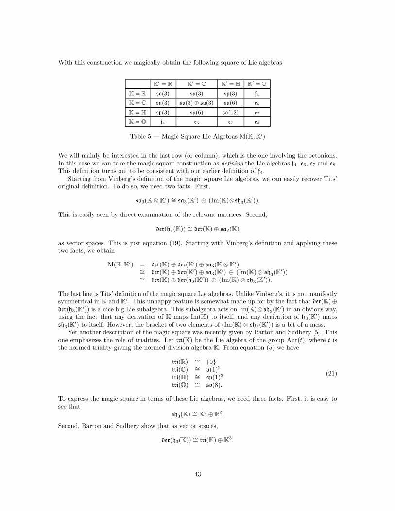
With this construction we magically obtain the following square of Lie algebras:

K′ = R K′ = C K′ = H K′ = OK = R so(3) su(3) sp(3) f4

K = C su(3) su(3)⊕ su(3) su(6) e6

K = H sp(3) su(6) so(12) e7

K = O f4 e6 e7 e8

Table 5 — Magic Square Lie Algebras M(K,K′)

We will mainly be interested in the last row (or column), which is the one involving the octonions.In this case we can take the magic square construction as defining the Lie algebras f4, e6, e7 and e8.This definition turns out to be consistent with our earlier definition of f4.

Starting from Vinberg’s definition of the magic square Lie algebras, we can easily recover Tits’original definition. To do so, we need two facts. First,

sa3(K⊗K′) ∼= sa3(K′) ⊕ (Im(K)⊗sh3(K′)).

This is easily seen by direct examination of the relevant matrices. Second,

der(h3(K)) ∼= der(K)⊕ sa3(K)

as vector spaces. This is just equation (19). Starting with Vinberg’s definition and applying thesetwo facts, we obtain

M(K,K′) = der(K)⊕ der(K′)⊕ sa3(K⊗K′)∼= der(K)⊕ der(K′)⊕ sa3(K′) ⊕ (Im(K)⊗ sh3(K′))∼= der(K)⊕ der(h3(K′)) ⊕ (Im(K)⊗ sh3(K′)).

The last line is Tits’ definition of the magic square Lie algebras. Unlike Vinberg’s, it is not manifestlysymmetrical in K and K′. This unhappy feature is somewhat made up for by the fact that der(K)⊕der(h3(K′)) is a nice big Lie subalgebra. This subalgebra acts on Im(K)⊗sh3(K′) in an obvious way,using the fact that any derivation of K maps Im(K) to itself, and any derivation of h3(K′) mapssh3(K′) to itself. However, the bracket of two elements of (Im(K)⊗ sh3(K′)) is a bit of a mess.

Yet another description of the magic square was recently given by Barton and Sudbery [5]. Thisone emphasizes the role of trialities. Let tri(K) be the Lie algebra of the group Aut(t), where t isthe normed triality giving the normed division algebra K. From equation (5) we have

tri(R) ∼= {0}tri(C) ∼= u(1)2

tri(H) ∼= sp(1)3

tri(O) ∼= so(8).

(21)

To express the magic square in terms of these Lie algebras, we need three facts. First, it is easy tosee that

sh3(K) ∼= K3 ⊕ R2.

Second, Barton and Sudbery show that as vector spaces,

der(h3(K)) ∼= tri(K)⊕K3.

43

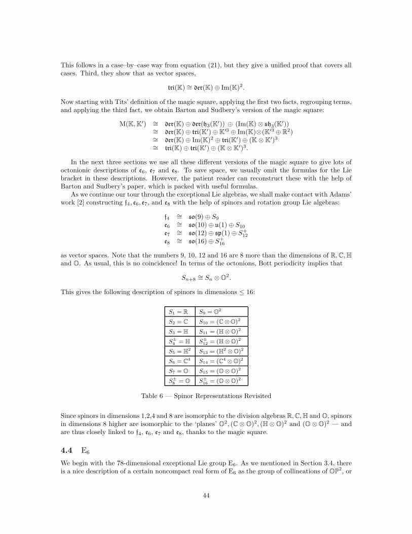
This follows in a case–by–case way from equation (21), but they give a unified proof that covers allcases. Third, they show that as vector spaces,

tri(K) ∼= der(K)⊕ Im(K)2.

Now starting with Tits’ definition of the magic square, applying the first two facts, regrouping terms,and applying the third fact, we obtain Barton and Sudbery’s version of the magic square:

M(K,K′) ∼= der(K)⊕ der(h3(K′)) ⊕ (Im(K)⊗ sh3(K′))∼= der(K)⊕ tri(K′)⊕K′3 ⊕ Im(K)⊗(K′3 ⊕ R2)∼= der(K)⊕ Im(K)2 ⊕ tri(K′)⊕ (K⊗K′)3

∼= tri(K)⊕ tri(K′)⊕ (K⊗K′)3.

In the next three sections we use all these different versions of the magic square to give lots ofoctonionic descriptions of e6, e7 and e8. To save space, we usually omit the formulas for the Liebracket in these descriptions. However, the patient reader can reconstruct these with the help ofBarton and Sudbery’s paper, which is packed with useful formulas.

As we continue our tour through the exceptional Lie algebras, we shall make contact with Adams’work [2] constructing f4, e6, e7, and e8 with the help of spinors and rotation group Lie algebras:

f4 ∼= so(9)⊕ S9

e6∼= so(10)⊕ u(1)⊕ S10

e7∼= so(12)⊕ sp(1)⊕ S+

12

e8∼= so(16)⊕ S+

16

as vector spaces. Note that the numbers 9, 10, 12 and 16 are 8 more than the dimensions of R,C,Hand O. As usual, this is no coincidence! In terms of the octonions, Bott periodicity implies that

Sn+8∼= Sn ⊗O2.

This gives the following description of spinors in dimensions ≤ 16:

S1 = R S9 = O2

S2 = C S10 = (C⊗O)2

S3 = H S11 = (H⊗O)2

S±4 = H S±12 = (H⊗O)2

S5 = H2 S13 = (H2 ⊗O)2

S6 = C4 S14 = (C4 ⊗O)2

S7 = O S15 = (O⊗O)2

S±8 = O S±16 = (O⊗O)2

Table 6 — Spinor Representations Revisited

Since spinors in dimensions 1,2,4 and 8 are isomorphic to the division algebras R,C,H and O, spinorsin dimensions 8 higher are isomorphic to the ‘planes’ O2, (C ⊗O)2, (H⊗O)2 and (O⊗O)2 — andare thus closely linked to f4, e6, e7 and e8, thanks to the magic square.

4.4 E6

We begin with the 78-dimensional exceptional Lie group E6. As we mentioned in Section 3.4, thereis a nice description of a certain noncompact real form of E6 as the group of collineations of OP2, or

44

equivalently, the group of determinant-preserving linear transformations of h3(O). But before goinginto these, we consider the magic square constructions of the Lie algebra e6. Vinberg’s constructiongives

e6 = der(O)⊕ sa3(C⊗O).

Tits’ construction, which is asymmetrical, gives

e6∼= der(h3(O))⊕ sh3(O)

and alsoe6∼= der(O)⊕ der(h3(C)) ⊕ (Im(O)⊗sh3(C)).

The Barton-Sudbery construction gives

e6∼= tri(O)⊕ tri(C)⊕ (C⊗O)3.

We can use any of these to determine the dimension of e6. For example, we have

dim(e6) = dim(der(h3(O))) + dim(sh3(O)) = 52 + 26 = 78.

Starting from the Barton-Sudbery construction and using the concrete descriptions of tri(O) andtri(C) from equation (21), we obtain

e6∼= so(O)⊕ so(C)⊕ Im(C)⊕ (C⊗O)3

Using equation (17), we may rewrite this as

e6∼= so(O⊕ C)⊕ Im(C)⊕ (C⊗O)2

and it turns out that the summand so(O⊕C)⊕ Im(C) is actually a Lie subalgebra of e6. This resultcan also be found in Adams’ book [2], phrased as follows:

e6∼= so(10)⊕ u(1)⊕ S10

In fact, he describes the bracket in e6 in terms of natural operations involving so(10) and its spinorrepresentation S10. The funny-looking factor of u(1) comes from the fact that this spinor represen-tation is complex. The bracket of an element of u(1) and an element of S10 is another element ofS10, defined using the obvious action of u(1) on this complex vector space.

If we define E6 to be the simply connected group with Lie algebra e6, it follows from results ofAdams that the subgroup generated by the Lie subalgebra so(10)⊕u(1) is isomorphic to (Spin(10)×U(1))/Z4. This lets us define the bioctonionic projective plane by

(C⊗O)P2 = E6 / ((Spin(10)×U(1))/Z4)

and conclude that the tangent space at any point of this manifold is isomorphic to S10∼= (C⊗O)2.

Since E6 is compact, we can put an E6-invariant Riemannian metric on the bioctonionic projectiveplane by averaging any metric with respect to the action of this group. It turns out [6] that theisometry group of this metric is exactly E6, so we have

E6∼= Isom((C⊗O)P2).

It follows thate6∼= isom((C⊗O)P2).

Summarizing, we have 6 octonionic descriptions of e6:

45

Theorem 6. The compact real form of e6 is given by

e6∼= isom((C⊗O)P2)∼= der(O)⊕ der(h3(C))⊕ (Im(O)⊗sh3(C))∼= der(h3(O))⊕ sh3(O)∼= der(O)⊕ sa3(C⊗O)∼= so(O⊕ C)⊕ Im(C)⊕ (C⊗O)2

∼= so(O)⊕ so(C)⊕ Im(C)⊕ (C⊗O)3

where in each case the Lie bracket of e6 is built from natural bilinear operations on the summands.

The smallest nontrivial representations of E6 are 27-dimensional: in fact it has two inequivalentrepresentations of this dimension, which are dual to one another. Now, the exceptional Jordanalgebra is also 27-dimensional, and in 1950 this clue led Chevalley and Schafer [21] to give a nicedescription of E6 as symmetries of this algebra. These symmetries do not preserve the product, butonly the determinant.

More precisely, the group of determinant-preserving linear transformations of h3(O) turns out tobe a noncompact real form of E6. This real form is sometimes called E6(−26), because its Killing formhas signature −26. To see this, note that any automorphism of h3(O) preserves the determinant, sowe get an inclusion

F4 ↪→ E6(−26).

This means that F4 is a compact subgroup of E6(−26). In fact it is a maximal compact subgroup, since

if there were a larger one, we could average a Riemannian metric group on OP2 with respect to thisgroup and get a metric with an isometry group larger than F4, but no such metric exists. It followsthat the Killing form on the Lie algebra e6(−26) is negative definite on its 52-dimensional maximalcompact Lie algebra, f4, and positive definite on the complementary 26-dimensional subspace, givinga signature of 26− 52 = −26.

We saw in Section 3.4 that the projective plane structure of OP2 can be constructed startingonly with the determinant function on the vector space h3(O). It follows that E6(−26) acts as

collineations on OP2, that is, line-preserving transformations. In fact, the group of collineationsof OP2 is precisely E6(−26):

E6(−26)∼= Coll(OP2).

Moreover, just as the group of isometries of OP2 fixing a specific point is a copy of Spin(9), thegroup of collineations fixing a specific point contains Spin(9, 1). This fact follows with some workstarting from equation (8), and it gives us a commutative square of inclusions:

Spin(9) −→ Isom(OP2) ∼= F4

↓ ↓Spin(9, 1) −→ Coll(OP2) ∼= E6(−26)

where the groups on the top are maximal compact subgroups of those on the bottom. Thus in avery real sense, F4 is to 9-dimensional Euclidean geometry as E6(−26) is to 10-dimensional Lorentziangeometry.

4.5 E7

Next we turn to the 133-dimensional exceptional Lie group E7. In 1954, Freudenthal [41] de-scribed this group as the automorphism group of a 56-dimensional octonionic structure now called

46

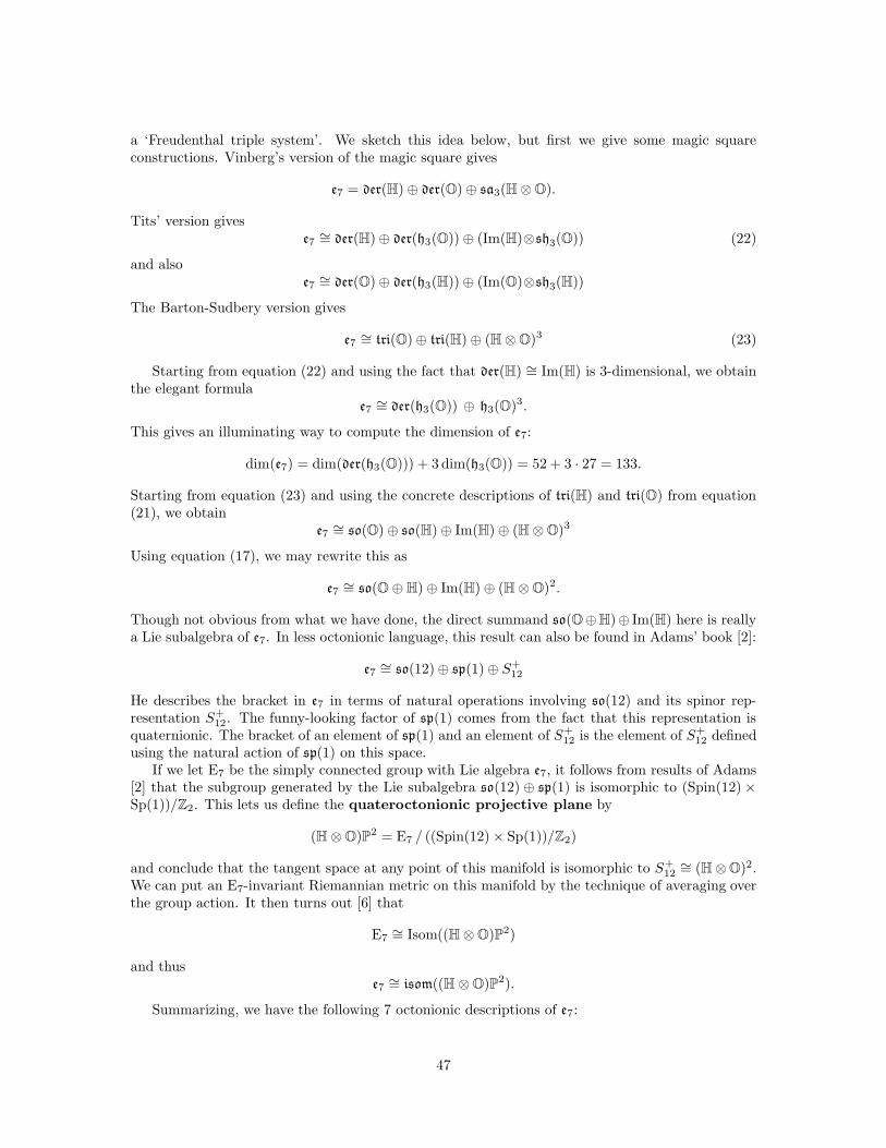
a ‘Freudenthal triple system’. We sketch this idea below, but first we give some magic squareconstructions. Vinberg’s version of the magic square gives

e7 = der(H)⊕ der(O)⊕ sa3(H⊗O).

Tits’ version givese7∼= der(H)⊕ der(h3(O))⊕ (Im(H)⊗sh3(O)) (22)

and alsoe7∼= der(O)⊕ der(h3(H))⊕ (Im(O)⊗sh3(H))

The Barton-Sudbery version gives

e7∼= tri(O)⊕ tri(H)⊕ (H⊗O)3 (23)

Starting from equation (22) and using the fact that der(H) ∼= Im(H) is 3-dimensional, we obtainthe elegant formula

e7∼= der(h3(O)) ⊕ h3(O)3.

This gives an illuminating way to compute the dimension of e7:

dim(e7) = dim(der(h3(O))) + 3 dim(h3(O)) = 52 + 3 · 27 = 133.

Starting from equation (23) and using the concrete descriptions of tri(H) and tri(O) from equation(21), we obtain

e7∼= so(O)⊕ so(H)⊕ Im(H)⊕ (H⊗O)3

Using equation (17), we may rewrite this as

e7∼= so(O⊕H)⊕ Im(H)⊕ (H⊗O)2.

Though not obvious from what we have done, the direct summand so(O⊕H)⊕ Im(H) here is reallya Lie subalgebra of e7. In less octonionic language, this result can also be found in Adams’ book [2]:

e7∼= so(12)⊕ sp(1)⊕ S+

12

He describes the bracket in e7 in terms of natural operations involving so(12) and its spinor rep-resentation S+

12. The funny-looking factor of sp(1) comes from the fact that this representation isquaternionic. The bracket of an element of sp(1) and an element of S+

12 is the element of S+12 defined

using the natural action of sp(1) on this space.If we let E7 be the simply connected group with Lie algebra e7, it follows from results of Adams

[2] that the subgroup generated by the Lie subalgebra so(12) ⊕ sp(1) is isomorphic to (Spin(12)×Sp(1))/Z2. This lets us define the quateroctonionic projective plane by

(H⊗O)P2 = E7 / ((Spin(12)× Sp(1))/Z2)

and conclude that the tangent space at any point of this manifold is isomorphic to S+12∼= (H⊗O)2.

We can put an E7-invariant Riemannian metric on this manifold by the technique of averaging overthe group action. It then turns out [6] that

E7∼= Isom((H⊗O)P2)

and thuse7∼= isom((H⊗O)P2).

Summarizing, we have the following 7 octonionic descriptions of e7:

47

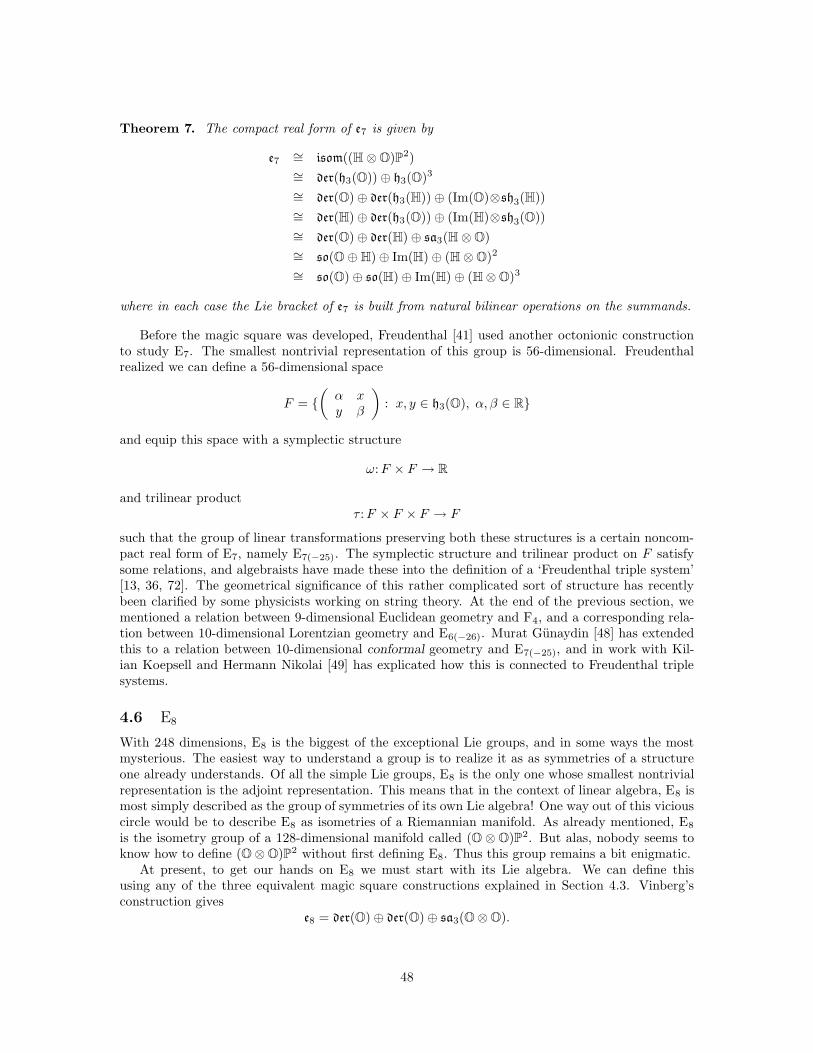
Theorem 7. The compact real form of e7 is given by

e7∼= isom((H⊗O)P2)∼= der(h3(O))⊕ h3(O)3

∼= der(O)⊕ der(h3(H))⊕ (Im(O)⊗sh3(H))∼= der(H)⊕ der(h3(O))⊕ (Im(H)⊗sh3(O))∼= der(O)⊕ der(H)⊕ sa3(H⊗O)∼= so(O⊕H)⊕ Im(H)⊕ (H⊗O)2

∼= so(O)⊕ so(H)⊕ Im(H)⊕ (H⊗O)3

where in each case the Lie bracket of e7 is built from natural bilinear operations on the summands.

Before the magic square was developed, Freudenthal [41] used another octonionic constructionto study E7. The smallest nontrivial representation of this group is 56-dimensional. Freudenthalrealized we can define a 56-dimensional space

F = {(α xy β

): x, y ∈ h3(O), α, β ∈ R}

and equip this space with a symplectic structure

ω:F × F → R

and trilinear productτ :F × F × F → F

such that the group of linear transformations preserving both these structures is a certain noncom-pact real form of E7, namely E7(−25). The symplectic structure and trilinear product on F satisfysome relations, and algebraists have made these into the definition of a ‘Freudenthal triple system’[13, 36, 72]. The geometrical significance of this rather complicated sort of structure has recentlybeen clarified by some physicists working on string theory. At the end of the previous section, wementioned a relation between 9-dimensional Euclidean geometry and F4, and a corresponding rela-tion between 10-dimensional Lorentzian geometry and E6(−26). Murat Gunaydin [48] has extendedthis to a relation between 10-dimensional conformal geometry and E7(−25), and in work with Kil-ian Koepsell and Hermann Nikolai [49] has explicated how this is connected to Freudenthal triplesystems.

4.6 E8

With 248 dimensions, E8 is the biggest of the exceptional Lie groups, and in some ways the mostmysterious. The easiest way to understand a group is to realize it as as symmetries of a structureone already understands. Of all the simple Lie groups, E8 is the only one whose smallest nontrivialrepresentation is the adjoint representation. This means that in the context of linear algebra, E8 ismost simply described as the group of symmetries of its own Lie algebra! One way out of this viciouscircle would be to describe E8 as isometries of a Riemannian manifold. As already mentioned, E8

is the isometry group of a 128-dimensional manifold called (O ⊗O)P2. But alas, nobody seems toknow how to define (O⊗O)P2 without first defining E8. Thus this group remains a bit enigmatic.

At present, to get our hands on E8 we must start with its Lie algebra. We can define thisusing any of the three equivalent magic square constructions explained in Section 4.3. Vinberg’sconstruction gives

e8 = der(O)⊕ der(O)⊕ sa3(O⊗O).

48

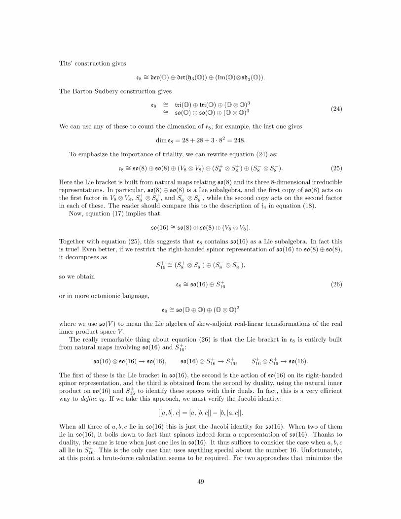
Tits’ construction gives

e8∼= der(O)⊕ der(h3(O))⊕ (Im(O)⊗sh3(O)).

The Barton-Sudbery construction gives

e8∼= tri(O)⊕ tri(O)⊕ (O⊗O)3

∼= so(O)⊕ so(O)⊕ (O⊗O)3 (24)

We can use any of these to count the dimension of e8; for example, the last one gives

dim e8 = 28 + 28 + 3 · 82 = 248.

To emphasize the importance of triality, we can rewrite equation (24) as:

e8∼= so(8)⊕ so(8)⊕ (V8 ⊗ V8)⊕ (S+

8 ⊗ S+8 )⊕ (S−8 ⊗ S−8 ). (25)

Here the Lie bracket is built from natural maps relating so(8) and its three 8-dimensional irreduciblerepresentations. In particular, so(8) ⊕ so(8) is a Lie subalgebra, and the first copy of so(8) acts onthe first factor in V8 ⊗ V8, S+

8 ⊗ S+8 , and S−8 ⊗ S−8 , while the second copy acts on the second factor

in each of these. The reader should compare this to the description of f4 in equation (18).Now, equation (17) implies that

so(16) ∼= so(8)⊕ so(8)⊕ (V8 ⊗ V8).

Together with equation (25), this suggests that e8 contains so(16) as a Lie subalgebra. In fact thisis true! Even better, if we restrict the right-handed spinor representation of so(16) to so(8)⊕ so(8),it decomposes as

S+16∼= (S+

8 ⊗ S+8 )⊕ (S−8 ⊗ S−8 ),

so we obtaine8∼= so(16)⊕ S+

16 (26)

or in more octonionic language,

e8∼= so(O⊕O)⊕ (O⊗O)2

where we use so(V ) to mean the Lie algebra of skew-adjoint real-linear transformations of the realinner product space V .

The really remarkable thing about equation (26) is that the Lie bracket in e8 is entirely builtfrom natural maps involving so(16) and S+

16:

so(16)⊗ so(16)→ so(16), so(16)⊗ S+16 → S+

16, S+16 ⊗ S+

16 → so(16).

The first of these is the Lie bracket in so(16), the second is the action of so(16) on its right-handedspinor representation, and the third is obtained from the second by duality, using the natural innerproduct on so(16) and S+

16 to identify these spaces with their duals. In fact, this is a very efficientway to define e8. If we take this approach, we must verify the Jacobi identity:

[[a, b], c] = [a, [b, c]]− [b, [a, c]].

When all three of a, b, c lie in so(16) this is just the Jacobi identity for so(16). When two of themlie in so(16), it boils down to fact that spinors indeed form a representation of so(16). Thanks toduality, the same is true when just one lies in so(16). It thus suffices to consider the case when a, b, call lie in S+

16. This is the only case that uses anything special about the number 16. Unfortunately,at this point a brute-force calculation seems to be required. For two approaches that minimize the

49

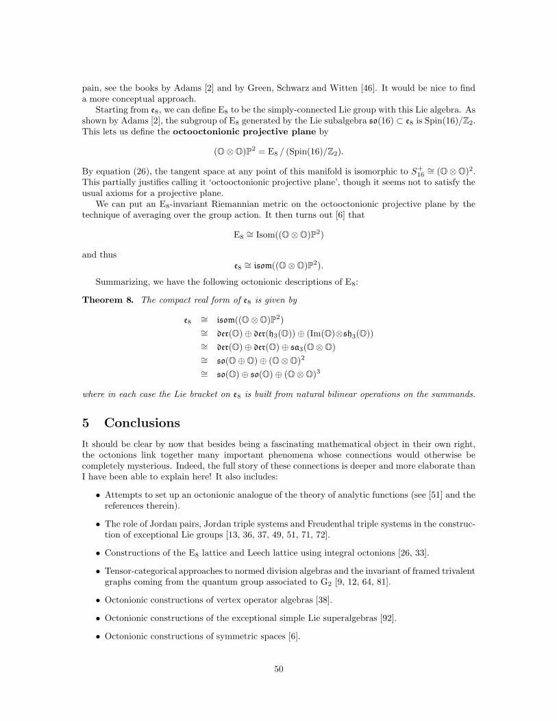
pain, see the books by Adams [2] and by Green, Schwarz and Witten [46]. It would be nice to finda more conceptual approach.

Starting from e8, we can define E8 to be the simply-connected Lie group with this Lie algebra. Asshown by Adams [2], the subgroup of E8 generated by the Lie subalgebra so(16) ⊂ e8 is Spin(16)/Z2.This lets us define the octooctonionic projective plane by

(O⊗O)P2 = E8 / (Spin(16)/Z2).

By equation (26), the tangent space at any point of this manifold is isomorphic to S+16∼= (O⊗O)2.

This partially justifies calling it ‘octooctonionic projective plane’, though it seems not to satisfy theusual axioms for a projective plane.

We can put an E8-invariant Riemannian metric on the octooctonionic projective plane by thetechnique of averaging over the group action. It then turns out [6] that

E8∼= Isom((O⊗O)P2)

and thuse8∼= isom((O⊗O)P2).

Summarizing, we have the following octonionic descriptions of E8:

Theorem 8. The compact real form of e8 is given by

e8∼= isom((O⊗O)P2)∼= der(O)⊕ der(h3(O))⊕ (Im(O)⊗sh3(O))∼= der(O)⊕ der(O)⊕ sa3(O⊗O)∼= so(O⊕O)⊕ (O⊗O)2

∼= so(O)⊕ so(O)⊕ (O⊗O)3

where in each case the Lie bracket on e8 is built from natural bilinear operations on the summands.

5 Conclusions

It should be clear by now that besides being a fascinating mathematical object in their own right,the octonions link together many important phenomena whose connections would otherwise becompletely mysterious. Indeed, the full story of these connections is deeper and more elaborate thanI have been able to explain here! It also includes:

• Attempts to set up an octonionic analogue of the theory of analytic functions (see [51] and thereferences therein).

• The role of Jordan pairs, Jordan triple systems and Freudenthal triple systems in the construc-tion of exceptional Lie groups [13, 36, 37, 49, 51, 71, 72].

• Constructions of the E8 lattice and Leech lattice using integral octonions [26, 33].

• Tensor-categorical approaches to normed division algebras and the invariant of framed trivalentgraphs coming from the quantum group associated to G2 [9, 12, 64, 81].

• Octonionic constructions of vertex operator algebras [38].

• Octonionic constructions of the exceptional simple Lie superalgebras [92].

• Octonionic constructions of symmetric spaces [6].

50

• Octonions and the geometry of the ‘squashed 7-spheres’, that is, the homogeneous spacesSpin(7)/G2, Spin(6)/SU(3), and Spin(5)/SU(2), all of which are diffeomorphic to S7 with itsusual smooth structure [22].

• The theory of ‘Joyce manifolds’, that is, 7-dimensional Riemannian manifolds with holonomygroup G2 [60].

• The octonionic Hopf map and instanton solutions of the Yang-Mills equations in 8 dimensions[47].

• Octonionic aspects of 10-dimensional superstring theory and 10-dimensional super-Yang-Millstheory [25, 29, 35, 65, 85, 86].

• Octonionic aspects of 11-dimensional supergravity and supermembrane theories, and the roleof Joyce manifolds in compactifying 11-dimensional supergravity to obtain theories of physicsin 4 dimensions [32].

• Geoffrey Dixon’s extension of the Standard Model based on the algebra C⊗H⊗O [31].

• Other attempts to use the octonions in physics [20, 51, 67, 76].

I urge the reader to explore these with the help of the references.

Acknowledgements

I thank John Barrett, Toby Bartels, Robert Bryant, Geoffrey Dixon, James Dolan, Tevian Dray,Bertram Kostant, Linus Kramer, Pertti Lounesto, Corinne Manogue, John McKay, David Rusin,Tony Smith, Anthony Sudbery, and Matthew Wiener for useful discussions.

References

[1] John F. Adams, On the non-existence of elements of Hopf invariant one, Ann. Math. 72 (1960),20–104.

[2] John F. Adams, Lectures on Exceptional Lie Groups, eds. Zafer Mahmud and Mamoru Mimira,University of Chicago Press, Chicago, 1996.

[3] Michael Atiyah and Friedrich Hirzebruch, Bott periodicity and the parallelizability of thespheres. Proc. Cambridge Philos. Soc. 57 (1961), 223–226.

[4] Helena Albuquerque and Shahn Majid, Quasialgebra structure of the octonions, preprint avail-able as math.QA/9802116.

[5] Chris H. Barton and Anthony Sudbery, Magic squares of Lie algebras, preprint available asmath.RA/0001083.

[6] Arthur L. Besse, Einstein Manifolds, Springer, Berlin, 1987, pp. 313–316.

[7] F. van der Blij, History of the octaves, Simon Stevin 34 (1961), 106—125.

[8] F. van der Blij and Tonny A. Springer, Octaves and triality, Nieuw Arch. v. Wiskunde 8 (1960),158–169.

[9] Dominik Boos, Ein tensorkategorieller Zugang zum Satz von Hurwitz, Diplomarbeit, ETHZurich, March 1998.

51

[10] Armand Borel, Le plan projectif des octaves et les spheres commes espaces homogenes, Compt.Rend. Acad. Sci. 230 (1950), 1378–1380.

[11] Raoul Bott and John Milnor, On the parallelizability of the spheres, Bull. Amer. Math. Soc.64 (1958) 87–89.

[12] Murray Bremner, Quantum octonions, Comm. Alg. 27 (1999), 2809–2831.

[13] Robert B. Brown, Groups of type E7, Jour. Reine Angew. Math. 236 (1969), 79–102.

[14] Elie Cartan, Sur la structure des groupes de tranformations finis et continus, These, Paris,Nony, 1894.

[15] Elie Cartan, Les groupes reels simples finis et continus, Ann. Sci. Ecole Norm. Sup. 31 (1914),255–262.

[16] Elie Cartan, Nombres complexes, in Encyclopedie des sciences mathematiques, 1, ed. J. Molk,1908, 329–468.

[17] Elie Cartan, Le principe de dualite et la theorie des groupes simple et semi-simples, Bull. Sci.Math. 49 (1925), 361–374.

[18] Arthur Cayley, On Jacobi’s elliptic functions, in reply to the Rev. B. Bronwin; and on quater-nions, Philos. Mag. 26 (1845), 208–211.

[19] Arthur Cayley, On Jacobi’s elliptic functions, in reply to the Rev. B. Bronwin; and on quater-nions (appendix only), in The Collected Mathematical Papers, Johnson Reprint Co., New York,1963, p. 127.

[20] Sultan Catto, Carlos J. Moreno and Chia-Hsiung Tze, Octonionic Structures in Physics, toappear.

[21] Claude Chevalley and Richard D. Schafer, The exceptional simple Lie algebras F4 and E6, Proc.Nat. Acad. Sci. USA 36 (1950), 137–141.

[22] Yvonne Choquet-Bruhat and Cecile DeWitt-Morette, Analysis, Manifolds and Physics, part II,Elsevier, Amsterdam, 2000, pp. 263–274.

[23] William K. Clifford, Applications of Grassmann’s extensive algebra, Amer. Jour. Math. 1(1878), 350–358.

[24] Frederick R. Cohen, On Whitehead squares, Cayley–Dickson algebras and rational functions,Bol. Soc. Mat. Mexicana 37 (1992), 55–62.

[25] E. Corrigan and T. J. Hollowood, The exceptional Jordan algebra and the superstring, Comm.Math. Phys. 122 (1989), 393–410.

[26] Harold Scott MacDonald Coxeter, Integral Cayley numbers, Duke Math. Jour. 13 (1946), 561–578.

[27] Michael J. Crowe, A History of Vector Analysis, University of Notre Dame Press, Notre Dame,1967.

[28] C. W. Curtis, The four and eight square problem and division algebras, in Studies in ModernAlgebra, ed. A. Albert, Prentice–Hall, Englewood Cliffs, New Jersey, 1963, pp. 100–125.

[29] Pierre Deligne et al, eds., Quantum Fields and Strings: A Course for Mathematicians, 2 volumes,Amer. Math. Soc., Providence, Rhode Island, 1999.

52

[30] Leonard E. Dickson, On quaternions and their generalization and the history of the eight squaretheorem, Ann. Math. 20 (1919), 155–171.

[31] Geoffrey M. Dixon, Division Algebras: Octonions, Quaternions, Complex Numbers and theAlgebraic Design of Physics, Kluwer, Dordrecht, 1994.

[32] M. J. Duff, ed., The World in Eleven Dimensions: Supergravity, Supermembranes and M-Theory, Institute of Physics Publishing, Bristol, 1999.

[33] Noam Elkies and Benedict H. Gross, The exceptional cone and the Leech lattice, Internat.Math. Res. Notices 14 (1996), 665–698.

[34] Gerard G. Emch, Algebraic Methods in Statistical Mechanics and Quantum Field Theory,Wiley-Interscience, New York, 1972.

[35] J. M. Evans, Supersymmetric Yang–Mills theories and division algebras, Nucl. Phys. B298(1988), 92–108.

[36] John R. Faulkner, A construction of Lie algebras from a class of ternary algebras, Trans. Amer.Math. Soc. 155 (1971), 397–408.

[37] John R. Faulkner and Joseph C. Ferrar, Exceptional Lie algebras and related algebraic andgeometric structures, Bull. London Math. Soc. 9 (1977), 1–35.

[38] Alex J. Feingold, Igor B. Frenkel, and John F. X. Ries, Spinor Construction of Vertex Operator

Algebras, Triality, and E(1)8 , Contemp. Math. 121, Amer. Math. Soc., Providence, Rhode Island,

1991.

[39] Hans Freudenthal, Oktaven, Ausnahmegruppen und Oktavengeometrie, mimeographed notes,1951. Also available in Geom. Dedicata 19 (1985), 7–63.

[40] Hans Freudenthal, Zur ebenen Oktavengeometrie, Indag. Math. 15 (1953), 195–200.

[41] Hans Freudenthal, Beziehungen der e7 und e8 zur Oktavenebene, I, II, Indag. Math. 16 (1954),218–230, 363–368. III, IV, Indag. Math. 17 (1955), 151–157, 277–285. V — IX, Indag. Math.21 (1959), 165–201, 447–474. X, XI, Indag. Math. 25 (1963) 457–487.

[42] Hans Freudenthal, Lie groups in the foundations of geometry, Adv. Math. 1 (1964), 145–190.

[43] Hans Freudenthal, Bericht uber die Theorie der Rosenfeldschen elliptischen Ebenen, inRaumtheorie, Wege Der Forschung, CCLXX, Wissenschaftliche Buchgesellschaft, Darmstadt,1978, pp. 283–286.

[44] Lynn E. Garner, An Outline of Projective Geometry, North Holland, New York, 1981.

[45] Robert Perceval Graves, Life of Sir William Rowan Hamilton, 3 volumes, Arno Press, NewYork, 1975.

[46] Michael B. Green, John H. Schwarz and Edward Witten, Superstring Theory, volume 1, Cam-bridge University Press, Cambridge, 1987, pp. 344–349.

[47] B. Grossman, T. E. Kephart, and James D. Stasheff, Solutions to Yang-Mills field equations ineight dimensions and the last Hopf map, Comm. Math. Phys. 96 (1984), 431–437.

[48] Murat Gunaydin, Generalized conformal and superconformal group actions and Jordan alge-bras, Mod. Phys. Lett. A8 (1993), 1407–1416.

53

[49] Murat Gunaydin, Kilian Koepsell, and Hermann Nicolai, Conformal and quasiconformal real-izations of exceptional Lie groups, preprint available as hep-th/0008063.

[50] Murat Gunaydin, C. Piron and H. Ruegg, Moufang plane and octonionic quantum mechanics,Comm. Math. Phys. 61 (1978), 69–85.

[51] Feza Gursey and Chia-Hsiung Tze, On the Role of Division, Jordan, and Related Algebras inParticle Physics, World Scientific, Singapore, 1996.

[52] William Rowan Hamilton, Four and eight square theorems, in Appendix 3 of The MathematicalPapers of William Rowan Hamilton, vol. 3, eds. H. Halberstam and R. E. Ingram, CambridgeUniversity Press, Cambridge, 1967, pp. 648–656.

[53] Thomas L. Hankins, Sir William Rowan Hamilton, John Hopkins University Press, Baltimore,1980.

[54] F. Reese Harvey, Spinors and Calibrations, Academic Press, San Diego, 1990.

[55] Adolf Hurwitz, Uber die Composition der quadratischen Formen von beliebig vielen Variabeln,Nachr. Ges. Wiss. Gottingen (1898) 309–316.

[56] Dale Husemoller, Fibre Bundles, Springer, Berlin, 1994.

[57] Pascual Jordan, Uber eine Klasse nichtassociativer hyperkomplexer Algebren, Nachr. Ges. Wiss.Gottingen (1932), 569–575.

[58] Pascual Jordan, Uber eine nicht-desarguessche ebene projektive Geometrie, Abh. Math. Sem.Hamburg 16 (1949), 74–76.

[59] Pascual Jordan, John von Neumann, Eugene Wigner, On an algebraic generalization of thequantum mechanical formalism, Ann. Math. 35 (1934), 29–64.

[60] Dominic Joyce, Compact Manifolds with Special Holonomy, Oxford U. Press, Oxford, 2000.

[61] I. L. Kantor and A. S. Solodovnikov, Hypercomplex Numbers — an Elementary Introductionto Algebras, Springer, Berlin, 1989.

[62] Michel Kervaire, Non-parallelizability of the n sphere for n > 7, Proc. Nat. Acad. Sci. USA 44(1958), 280–283.

[63] Wilhelm Killing, Die Zusammensetzung der stetigen endlichen Transformationsgruppen I, Math.Ann. 31 (1888), 252–290. II, 33 (1889) 1–48. III, 34 (1889), 57–122. IV 36 (1890), 161–189.

[64] Greg Kuperberg, Spiders for rank 2 Lie algebras, Comm. Math. Phys. 180 (1996), 109–151.

[65] T. Kugo and P.–K. Townsend, Supersymmetry and the division algebras, Nucl. Phys. B221(1983), 357–380.

[66] J. M. Landsberg and L. Manivel: The projective geometry of Freudenthal’s magic square,preprint available as math.AG/9908039.

[67] Jaak Lohmus, Eugene Paal, and Leo Sorgsepp, Nonassociative Algebras in Physics, HadronicPress, Palm Harbor, Florida, 1994.

[68] Corinne A. Manogue and Tevian Dray, Octonionic Mobius transformations, Mod. Phys. Lett.A14 (1999), 1243–1256.

[69] Corinne A. Manogue and Jorg Schray, Finite Lorentz transformations, automorphisms, anddivision algebras, Jour. Math. Phys. 34 (1993), 3746–3767.

54

[70] Corinne A. Manogue and Jorg Schray, Octonionic representations of Clifford algebras and tri-ality, Found. Phys. 26 (1996), 17–70.

[71] Kevin McCrimmon, Jordan algebras and their applications, Bull. Amer. Math. Soc. 84 (1978),612–627.

[72] K. Meyberg, Eine Theorie der Freudenthalschen Tripelsysteme, I, II, Indag. Math. 30 (1968),162–190.

[73] R. Guillermo Moreno, The zero divisors of the Cayley–Dickson algebras over the real numbers,preprint available at q-alg/9710013.

[74] Ruth Moufang, Alternativkorper und der Satz vom vollstandigen Vierseit, Abh. Math. Sem.Hamburg 9 (1933), 207–222.

[75] A. L. Onishchik and E. B. Vinberg, eds., Lie Groups and Lie Algebras III, Springer, Berlin,1991, pp. 167–178.

[76] Susumu Okubo, Introduction to Octonion and Other Non-Associative Algebras in Physics,Cambridge University Press, Cambridge, 1995.

[77] Roger Penrose and Wolfgang Rindler, Spinors and Space-Time, 2 volumes, Cambridge U. Press,Cambridge, 1985-86.

[78] Ian R. Porteous, Topological Geometry, Cambridge U. Press, 1981.

[79] Boris A. Rosenfeld, Geometrical interpretation of the compact simple Lie groups of the class E(Russian), Dokl. Akad. Nauk. SSSR (1956) 106, 600-603.

[80] Boris A. Rosenfeld, Geometry of Lie Groups, Kluwer, Dordrecht, 1997.

[81] Markus Rost, On the dimension of a composition algebra, Doc. Math. 1 (1996), 209–214.

[82] Helmut Salzmann et al, Compact Projective Planes: With an Introduction to Octonion Geom-etry, de Gruyter, Berlin, 1995.

[83] Richard D. Schafer, On algebras formed by the Cayley–Dickson process, Amer. Jour. of Math.76 (1954) 435–446.

[84] Richard D. Schafer, Introduction to Non-Associative Algebras, Dover, New York, 1995.

[85] Jorg Schray, Octonions and Supersymmetry, Ph.D. thesis, Department of Physics, Oregon StateUniversity, 1994.

[86] G. Sierra, An application of the theories of Jordan algebras and Freudenthal triple systems toparticles and strings, Class. Quant. Grav. 4 (1987), 227–236.

[87] Tonny A. Springer, The projective octave plane, I–II, Indag. Math. 22 (1960), 74–101.

[88] Tonny A. Springer, Characterization of a class of cubic forms, Indag. Math. 24 (1962), 259–265.

[89] Tonny A. Springer, On the geometric algebra of the octave planes, Indag. Math. 24 (1962),451–468.

[90] Tonny A. Springer and Ferdinand D. Veldkamp, Octonions, Jordan Algebras and ExceptionalGroups, Springer, Berlin, 2000.

[91] Frederick W. Stevenson, Projective Planes, W. H. Freeman and Company, San Francisco, 1972.

55

[92] Anthony Sudbery, Octonionic description of exceptional Lie superalgebras, Jour. Math. Phys.24 (1983), 1986–1988.

[93] Anthony Sudbery, Division algebras, (pseudo)orthogonal groups and spinors, Jour. Phys. A17(1984), 939–955.

[94] Jacques Tits, Le plan projectif des octaves et les groupes de Lie exceptionnels, Bull. Acad. Roy.Belg. Sci. 39 (1953), 309–329.

[95] Jacques Tits, Le plan projectif des octaves et les groupes exceptionnels E6 et E7, Bull. Acad.Roy. Belg. Sci. 40 (1954), 29–40.

[96] Jacques Tits, Algebres alternatives, algebres de Jordan et algebres de Lie exceptionnelles, Indag.Math. 28 (1966), 223–237.

[97] Jacques Tits, Buildings of Spherical Type and Finite BN-Pairs, Lecture Notes in Mathematics,Vol. 386, Springer, Berlin, 1974.

[98] V. S. Varadarajan, Geometry of Quantum Theory, Springer-Verlag, Berlin, 1985.

[99] E. B. Vinberg, A construction of exceptional simple Lie groups (Russian), Tr. Semin. Vektorn.Tensorn. Anal. 13 (1966), 7–9.

[100] Max Zorn, Theorie der alternativen Ringe, Abh. Math. Sem. Univ. Hamburg 8 (1930), 123–147.

[101] Max Zorn, Alternativkorper und quadratische Systeme, Abh. Math. Sem. Univ. Hamburg 9(1933), 395–402.

56