1. Introduction.

The importance of rapid ambulance response to emergency medical crises has been

well-documented. Indeed, according to the American Heart Association, early access to

advanced care is a crucial link in the Cardiac Chain of Survival1. A study in Ontario,

Canada concluded that in order to improve survival rates after cardiac arrest, ambulance

response times must be reduced and the frequency of bystander-initiated CPR increased2.

A study performed in King County, Washington determined survival rate to decrease by

2.1% per minute without intervention by Advanced Cardiac Life Support (ACLS) 3

.

Urban response time in a Southwestern metropolitan county of population 620,000 was

correlated with myocardial infarction survival rate, and it was found that a response time

of under 5 minutes would have a beneficial impact on survival4. Similarly, studies have

shown that response time and transport time are correlated with survival rates for

abdominal gunshot wound victims, and that the overall total Emergency Medical Services

(EMS) pre-hospital time interval was significantly lower for trauma survivors than for

non-survivors5,6

.

While any decrease in ambulance response time is likely to be beneficial, several

studies have taken the approach of spatial-temporal modeling of response times in order

to identify particular areas where improvements might have the most effect. For

instance, a study of response times in Houston, Texas used a queuing model to show that

increased dispersion of ambulances in areas away from those of high demand improves

the tail of the response time distribution7. Similarly, a computer-based model developed

for Los Angeles County was able to reliably predict response time and search for an

optimum pattern of ambulance deployment in order to minimize mean response time as

well as response time excesses8.

The goal of this paper is to investigate the dependence of ambulance response time on

system load. For a fixed region with a finite number of ambulances, one may anticipate

that response times may increase during times when a substantial portion of the

ambulances are unavailable due to previous emergencies. The focus of this paper is on

the spatial-temporal pattern of response times in Santa Barbara County, California,

during 2006, and particular attention is paid to the impact of the number of spatial-

temporally proximate emergency calls on response times.

2. Materials and Methods.

Santa Barbara County ambulance dispatch data for the year 2006 were provided by

Santa Barbara’s EMS agency for the UCLA Statistics Department’s EMS study group.

All analysis of the data is done using the R Language and Environment for Statistical

Computing [9]. Variables recorded include the incident time, geographical address,

incident type, response code, response district, response district type, ambulance dispatch

time, ambulance on scene time, hospital arrival time, and incident clear time. The

addresses were geocoded by the EMS study group using Yahoo! Geocoder into longitude

and latitude coordinates, and subsequently transformed into kilometer units using the

universal mercator transformation.

As measures of ambulance response performance, both response time and response

time regulation compliance were used, with ambulance response times defined as the

time elapsed between ambulance dispatch and ambulance on scene arrival. Events for

which ambulance response time could not be determined due to missing data were

excluded. Events where the location could not be determined are excluded from analysis

as well. Finally, since the focus of this study is on emergency calls, only Code 2 and

Code 3 dispatched calls were considered. Codes 3 and 2 refer to emergency calls where

ambulances respond with or without lights and sirens, respectively10

. In all there

remained a total of 21,944 emergency ambulance dispatch events in 2006 of which

15,883 (72.4%) were Code 3 responses and 6,061 (27.6%) were Code 2 responses.

The distribution of response times varies according to the response code and the

response zone type (Figure 1). With this in mind, Santa Barbara County adapted response

time regulations dependent upon population density and response code effective January

2005 governing response time standards and enforcement (Table 1). Overall, 95.1% of

Code 2 and Code 3 ambulance responses had response times within the limits set by these

regulations. Of the 861 events that were in violation of the regulations, 564 (65.5%) were

Code 3 events and 297 (34.5%) were Code 2 events. In total, 3.55% of Code 3 calls had

response times in violation, compared with 4.90% of Code 2 calls.

As a measure of system load at the time of each call, we define the statistic ß for each

call, as follows. If {(ti, xi); i = 1, ..., 21,944} represents the collection of times (ti) and

locations (x i) of recorded calls, let ßi(∆t , ∆x) = ∑ j < i 1{ti - tj ≤ ∆t} 1{d(xi , xj) ≤ ∆x},

where 1 denotes the indicator function, and d(xi , xj) denotes the spatial distance between

locations xi and xj. Thus ßi(∆t , ∆x) represents the number of calls prior to call i that were

within ∆t hours and within ∆x km of call i; such calls are subsequently referred to as

predecessors of call i.

After many choices of the parameters ∆t and ∆x were inspected, particular attention was

focused on the case where ∆t = 1 hour and ∆x = 20km, which appears to have the highest

correlation with response time. The parameter ∆x may be interpreted as an approximation

of the average area of an ambulance dispatch region, while a possible interpretation of

∆t may be the mean time required for an ambulance to return to service after it has been

dispatched to a previous call.

If M represents the total number of ambulances available for service in a particular area,

and k represents the number of ambulances that are actively responding to incidents, then

M-k is the number of ambulances in service that are available to respond to new calls.

One would expect response time to depend less heavily on k in regions where M is larger.

Similarly, in such regions, one would anticipate a one-unit increase in ß to be associated

with a smaller increase in mean response times for such regions.

To see how variation in the number ß of predecessors is associated with response time,

the incidents were first blocked for response code and district type. Within each block,

incident response times are sorted in ascending order, and the relationship between ß and

response time was smoothed using a moving average (MA) filter.

Response time regulations effective January 2005 provided standards for the timeliness

of an ambulance response given its response code and the population density of the area

of the emergency to which it is responding. From these regulations it was determined

whether or not each dispatch event was in compliance with the standard. A one-sided

Fisher's exact test was used to determine whether the proportion of violations was

significantly greater for incidents where ß>0, compared with incidents where ß=0. The

relationship between the number of predecessors and the probability of a violation was

summarized using logistic regression.

The spatial call distribution was estimated non-parametrically using kernel intensity

estimation, with an edge-corrected, isotropic Gaussian kernel11

. Due to geo-coding

precision inaccuracies, 24 call incidents lay outside of Santa Barbara County boundaries;

for the kernel intensity estimate, these points were excluded.

One aim of the present study is to look for evidence of spatial clustering of violation

incidents, and in particular for clustering of violation incidents which had a positive

number of predecessors. The inhomogeneous K-function was used for these purposes12

.

The inhomogeneous K-function can be used as a measure of the degree of clustering or

inhibition in points above and beyond what one would expect from a baseline model13

.

Here, we used the kernel estimate of the call rate at each location, scaled by the

proportion of calls which were violations, as a baseline model. Since many of the points

in the data set lie near the county borders, the choice of edge correction technique may

have a substantial impact on the estimated inhomogeneous K-function, so a variety of

edge-correction methods were used11,14

.

To identify areas where ß shows more of an effect on the proportion of violations, the

fraction of calls that were violations among calls with predecessors was compared with

the same fraction among calls without predecessors, for each spatial-temporal sub-region.

This difference was computed for all calls within 4 kilometers of each incident, provided

there were at least 10 incidents within 4 kilometers. These reflect regions that might

benefit the most from increased ambulance units or from optimizing the deployment

pattern of existing ambulances.

An exponential distribution was fitted to the distribution of incident inter-arrival times,

which are defined simply as the elapsed time between each incident and the event

preceding it. The exponential distribution for inter-arrival times is consistent with a time-

homogeneous Poisson process for call arrivals. As an alternative to the time-

homogeneous Poisson process, we considered an inhomogeneous Poisson process with

the temporal rate given by a kernel density estimate of the call times.

All multiple hypothesis testing was performed controlling family-wise error rate at

α=0.05 using Holm's stepwise p-value correction15

.

3. Results.

Figure 2 shows the distribution of the number ß of predecessors, within the previous

hour and within a radius of twenty km, for all Code 2 and Code 3 events in 2006. The

rapid decrease in frequency of calls with number of predecessors is readily evident in

Figure 2. The majority (68.5%) of events have fewer than 2 predecessors, and less than

2% of calls have more than 4 predecessors.

For calls where ß=0, i.e. calls without predecessors within 1hr and within 20km,

the proportion of response time violations was 2.96%, whereas for calls with ß>0, the

proportion of violations was 4.56%. The increase in probability of violation associated

with having predecessors is highly significant (Fisher's exact test; p = 7.2 x 10-10

). As ß

increases, both the response time and the probability of a response time violation were

seen to increase. The fit of a logistic regression model to the relationship between

violation and ß implies that on average, for each additional predecessor, the log odds ratio

log{p ÷ (1-p)} of the probability of violation increased by 19.1% (p = 6.3 x 10-11

). The

increase in response time associated with increasing ß is seen in Figure 3, which shows

the response time as a function of number of predecessors, smoothed using a moving

average (MA) filter. The positive association between ß and response time across

different response codes and population densities is evident in Figure 3. However, the

difference in probability of violation associated with changing ß is seen to vary across

response codes and district types. The increase in proportion of violations is most

pronounced in semi-rural calls, and its impact is slightly greater among Code 3 violations

rather than Code 2 violations.

Overall, the inter-arrival times between calls follows approximately an exponential

distribution with a rate of 2.51 calls per hour. The rate of call arrivals seems to vary,

however, according to the time of day, with the highest frequency of calls at mid-day.

Indeed, the frequency of calls is between 9am and 6pm is approximately three times

higher than that between 2am and 6am (Figure 4). Not surprisingly, the proportion of

calls where ß>0 varies according to the time of day as well. A multiple-comparison one-

sided Fisher's exact test shows that for the hours 9-10am, 12-1pm, 5-6pm, 8-9pm, and 10-

11pm, there is a statistically significantly higher proportion of calls that have

predecessors. The difference in proportion of calls that were violations for ß=0 and ß>0

varies according to the hour of day as well (Figure 5), with the highest proportion

between 6-7am and between 5-6pm, perhaps due to traffic incidence. In Figure 5, the

calls are divided into two categories: those for which the number ß of predecessors is

positive and those for which ß is zero. One sees that certain hours appear to have a

greater predecessor effect than others. For instance, between 6am and 8am, 5-6pm, 8-

9pm, and 11pm-11:59pm, the proportion of calls with ß > 0 that are violations is much

higher than that for calls with ß = 0. By contrast, during other hours the proportions are

similar, and between 4am and 5am, the proportion of calls that are violations is actually

higher for calls without predecessors than for calls with predecessors, perhaps due to lack

of available personnel.

The spatial distribution of ambulance response events consists of several areas of high

concentration, surrounded by vast areas of very low concentration, within the 9814 km^2

that comprise Santa Barbara County. Figure 6 shows a kernel intensity estimate of the

spatial call rates. One sees that the vast majority of calls are clustered within the main

urban parts of Santa Barbara County, especially in the cities of Santa Barbara,

Carpinteria, and Goleta (in the South-East), with one cluster in Santa Maria (in the North-

West), and another in Lompoc (toward the South-West).

Using the inhomogeneous K-function, one can assess the extent to which the observed

points exhibit significant clustering beyond what one would expect from an

inhomogeneous Poisson process. The inhomogeneous K-function, for calls which were in

violation and which had a positive number of predecessors, is shown in Figure 7.

It is clear from Figure 7 that there are areas where violations are more likely to coincide

with predecessors than expected under the null hypothesis that the violations occur

according to an inhomogeneous Poisson process. Hence the relationship between system

load and occurrence of response time violations is not only inhomogeneous in time, but

in space as well. To highlight this effect, Figure 8 shows the spatial distribution of

violations, organized according to the number of predecessors for each call, and Figure 9

shows the same for all calls. Essentially, the inhomogeneous K-function in Figure 7

suggests that the distributions shown in Figures 8 and 9 are significantly different, i.e.

that the violations are more clustered at a scale of 0-3 km than one would expect if they

were randomly sampled from the distribution of all calls.

Since there is spatial clustering in the points where calls with predecessors were

violations, it is useful to identify areas where this clustering is occurring. Locally, the

difference in proportion of violations between ß=0 and ß>0 ambulance responses was

calculated. This was done by calculating the difference for a radius of 4 km about each

location, provided that at least 10 calls had occurred within 4 km of the location in

question. Contours were drawn around regions where the difference in proportion

of violations was 5% or greater for Code 3 calls, and 3% or greater for Code 2 calls, and

the results are presented in Figures 10-11. The regions within these contours have a

statistically significantly greater proportion of violations for calls where ß>0 than calls

where ß=0. These regions represent areas where ambulance response time appears to be

significantly more sensitive to system load than elsewhere.

4. Discussion.

For calls which were preceded by at least one other call within the previous hour and

within 20km, the proportion that are violations is 4.56% compared with 2.96% for calls

without such predecessors. This 54% increase in the probability of a violation is perhaps

not surprising, since the role of system load on the incidence of violations is well known.

It is somewhat surprising, however, that this effect of preceding calls seems to be

especially pronounced during busy morning and evening commuting hours, whereas

during the very early morning (2-5am), the effect is negligible or perhaps even slightly

reversed. A possible explanation for this may be that violations in such nighttime hours

may be more closely related to the lack of any nearby personnel on duty, rather than

unavailability due to system load.

The impact of system load is also seen in the fact that the violations themselves are

significantly clustered, even after accounting for clustering due to population

inhomogeneity. Indeed, at a scale of 0-3km, it appears that violations are significantly

more clustered than one would expect if these calls were a random sampling from all

calls. It is difficult to think of an explanation for this observation other than the influence

of system load. This effect appears to be especially pronounced within semi-rural

neighborhoods.

Santa Barbara County is a somewhat unique blend of urban and rural neighborhoods,

with few locations of extremely high population density and also few locations that are

extremely far from any urban neighborhood. Extension of the present analysis to larger

domains and to domains other than Santa Barbara are important directions for future

work.

References:

1. Cummins RO, Ornato JP, Thies WH, Pepe PE. Improving survival from sudden

cardiac arrest: the 'chain of survival' concept. A statement for health professionals

from the Advanced Cardiac Life Support Subcommittee and the Emergency

Cardiac Care Committee, American Heart Association. Circulation 1991;

83:1832--1847.

2. References S, Brison R, Davidson R, Dreyer J, Rowe B. Cardiac arrest in Ontario:

circumstances, community response, role of prehospital defibrillation and

predictors of survival. Canadian Medical Association Journal 1992; 147: 191--

199.

3. Larsen MP, Eisenberg MS, Cummins RO, Hallstrom AP. Predicting survival from

out-of-hospital cardiac arrest: a graphic model. Annals of Emergency

Medicine1993; 22: 1652--1658.

4. Blackwell TH, Kaufman JS. Response time effectiveness: comparison of response

time and survival in an urban emergency medical services system. Academic

Emergency Medicine 2002; 9: 288.

5. Fiedler MD, Jones LM, Miller SF, Finley RK. A correlation of response time and

results of abdominal gunshot wounds. Archives of Surgery 1986; 121: 902--904.

6. Feero S, Hedges JR, Simmons E, Irwin L. Does out-of-hospital EMS time affect

trauma survival? American Journal of Emergency Medicine 1995; 13: 133--135.

7. Scott DW, Factor LE, Gorry GA. Predicting the response time of an urban ambulance

system. Health Serv. Res. 1978; 13: 404--417.

8. Fitzsimmons JA. A methodology for emergency ambulance deployment. Management

Science 1973; 19: 627--636.

9. R Development Core Team. R: A Language and Environment for Statistical

Computing. Vienna, Austria: R Foundation for Statistical Computing; 2007.

10. Ho J, Casey B.Time saved with use of emergency warning lights and sirens during

response to requests for emergency medical aid in an urban environment. Annals

of Emergency Medicine 1998; 32: 585--588.

11. Silverman BW. Density Estimation. London: Chapman and Hall; 1986.

12. Baddeley A, M{o}ller J, Waagepetersen R. Non-and semi-parametric estimation of

interaction in inhomogeneous point patterns. Statistica Neerlandica 2000; 54:

329--350.

13. Veen A, Schoenberg FP. Assessing spatial point process models using weighted K-

functions: analysis of California earthquakes. In: Baddeley A, Gregori P, Mateu

J, Stoica R, Stoyan D, eds. Lecture Notes in Statistics. New York NY: Springer;

2005: 269--297.

14. Ripley BD. Statistical Inference for Spatial Processes. Cambridge: Cambridge

University Press; 1988.

15. Holm S. A simple sequentially rejective multiple test procedure. Scandinavian

Journal of Statistics 1979; 6: 65--67.

Response Code Population Density First Responder Ambulance Arrival

Code 3 Urban < 8 min. < 10 min.

Code 3 Semi-rural < 15 min. < 17 min.

Code 3 Rural < 30 min. < 33 min.

Code 2 Urban < 15 min. < 17 min.

Code 2 Semi-rural < 25 min. < 27 min.

Code 2 Rural < 40 min. < 43 min.

Table 1: Conditions for compliance (non-violation status), depending on response code

and population density, according to Santa Barbara County ambulance response time

regulations effective January 2005.

FIGURE CAPTIONS:

Figure 1. Kernel density estimates of response times, across different Code and area

types.

Figure 2. Histogram of the number of predecessors (ß) within 20 kilometers and within

the previous hour of recorded calls.

Figure 3. Number of predecessors (ß) versus response time, for different Code and area

types. Results for ß and response time are averaged within pixels, and filtered using a

moving average (MA) filter.

Figure 4. Total Code 2 and Code 3 dispatch events for 2006 by hour of incidence.

Figure 5. Proportion of calls which are violations by hour of day, for calls with

predecessors (shaded bins) and for calls without predecessors (unshaded bins).

Figure 6. Kernel density estimate of the number of calls per squared kilometer over 2006.

An isotropic Gaussian kernel was used. The points overlaid are the call locations.

Figure 7. Inhomogeneous K-function for calls which were violations and which had

predecessors.

Figure 8. Maps of call locations, sorted by number of predecessors.

Figure 9. Localized increase in probability of Code 2 violation for calls with predecessors

versus calls without predecessors. Shown is a smoothed plot of the proportion of Code 2

calls with ß > 0 which were violations minus the proportion of Code 2 calls with ß = 0

which were violations.

Figure 10. Smoothed plot of the proportion of Code 3 calls with ß > 0 which were

violations minus the proportion of Code 3 calls with ß = 0 which were violations.

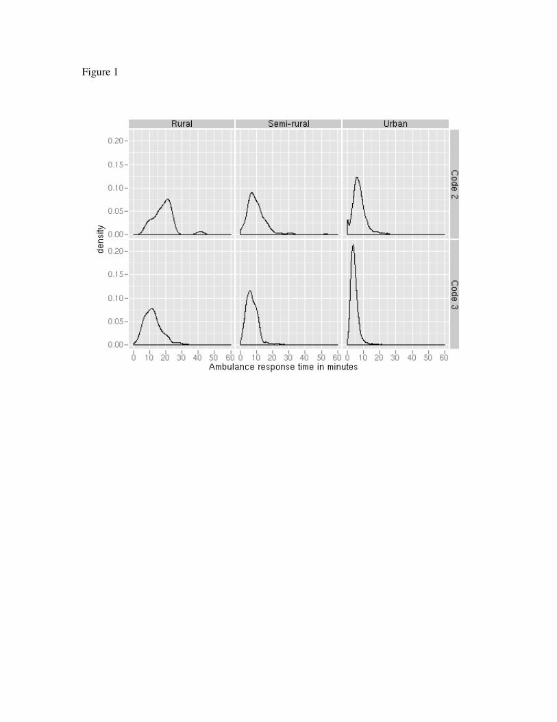
Figure 1

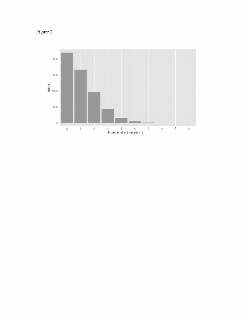
Figure 2

Figure 3

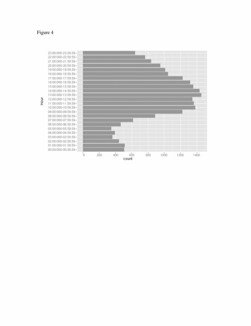
Figure 4

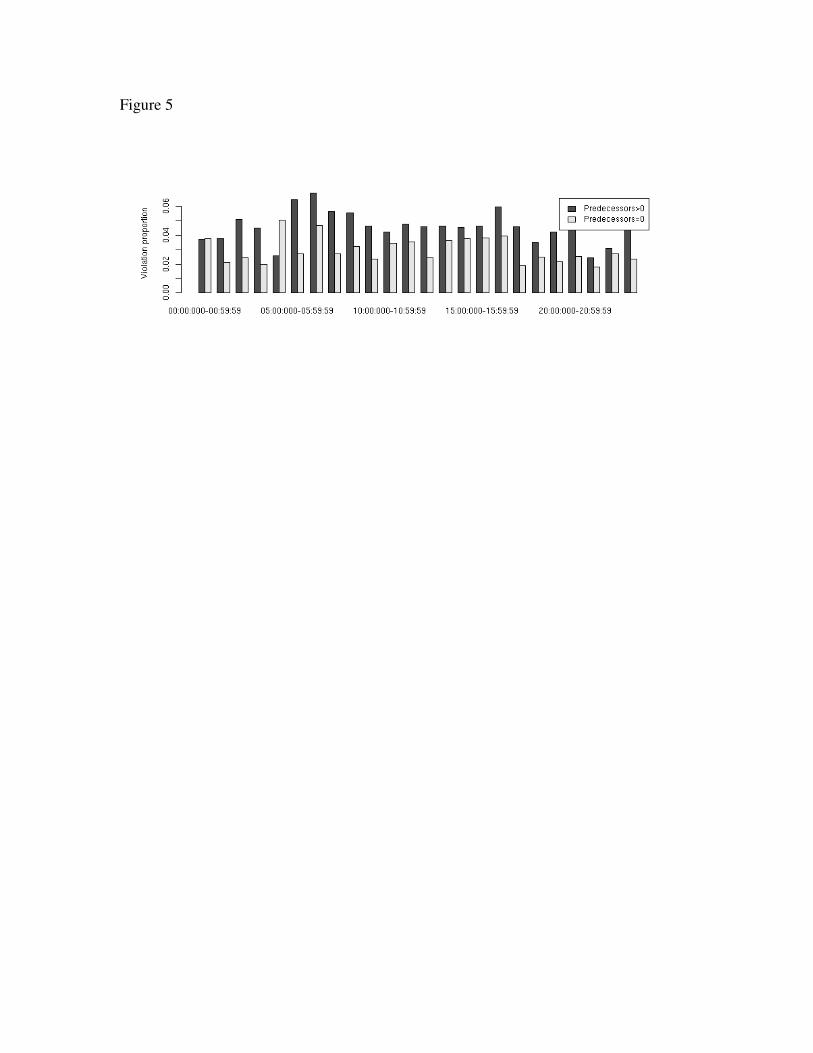
Figure 5

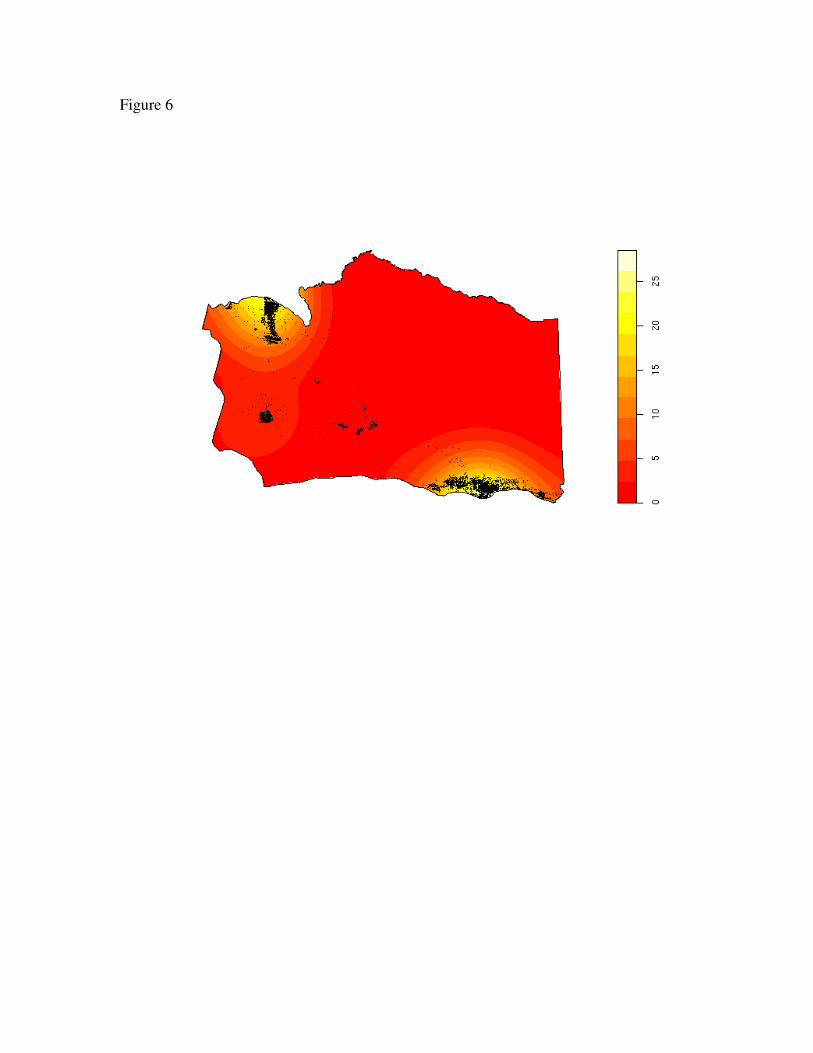
Figure 6

Figure 7

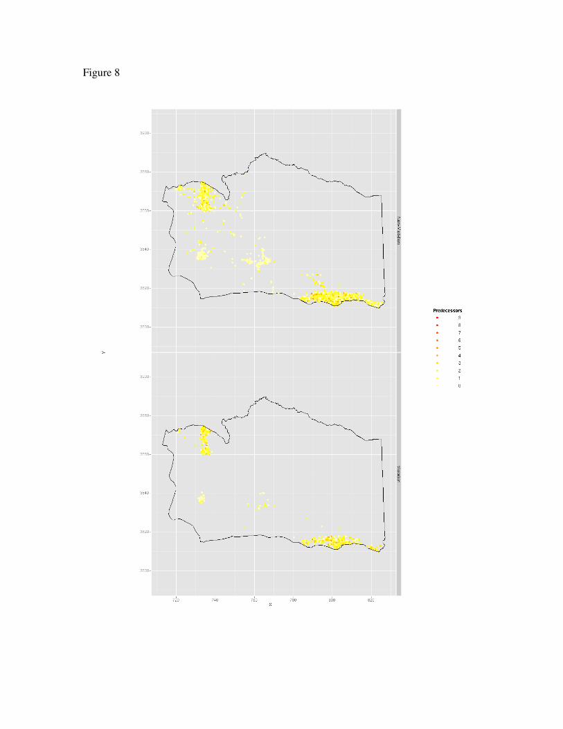
Figure 8

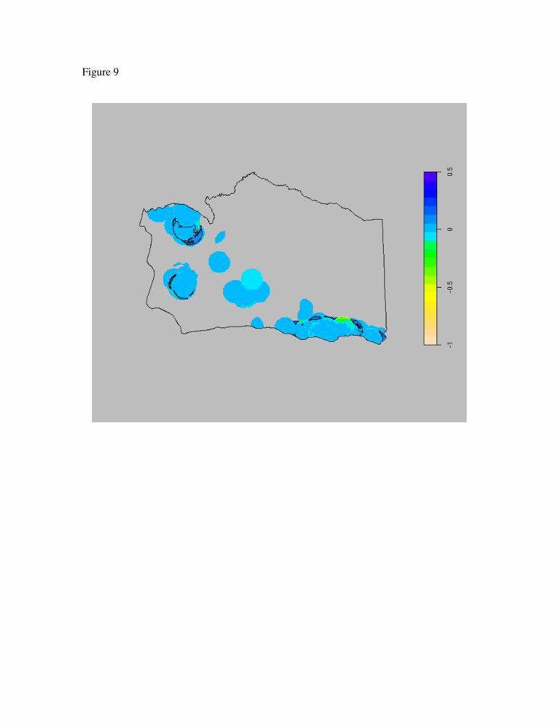
Figure 9

Figure 10