Embed Size (px)
Citation preview

1
Investigating M3 money demand in the euro area Christian Dreger and Jürgen Wolters 1
Abstract: Monetary growth in the euro area has exceeded its target since 2001. Like
wise, recent empirical studies did not find evidence in favour of a stable long run money
demand function. The equation appears to be increasingly unstable if more recent data
are used. If the link between money balances and the macroeconomy is fragile, the ra
tionale of monetary aggregates in the ECB strategy has to be doubted. In contrast to the
bulk of the literature, we are able to identify a stable long run money demand relation
ship, where recursively estimated parameters are almost constant. This result can be
obtained when the analysis is done without imposing a short run homogeneity restric
tion between money and prices. The corresponding error correction model survives a
huge battery of specification tests. The basic equation can be further improved by allow
ing for asymmetric adjustment. Due to a period of low inflation, opportunity costs of
holding money have decreased. Thus, the apparent monetary overhang can be recon
ciled within standard models of money demand.
Keywords: Cointegration analysis, error correction, asymmetric adjustment, money de
mand, monetary policy
JEL Classification: C22, C52, E41
1 Dreger: German Institute for Economic Research (DIW Berlin), KöniginLuiseStr. 5, D10551 Berlin, [email protected], Wolters: Freie Universität Berlin, Boltzmannstr. 20, D14195 Berlin, wolters@wiwiss. fuberlin.de.
2
1 Introduction
Monetary aggregates play a crucial role in the alignment of the two pillar monetary pol
icy strategy of the ECB. One pillar is based on the economic analysis of price risks in
the short term, and the other pillar includes the monetary analysis of risks to price sta
bility in the medium and long term (ECB, 2003). The reference value for monetary
growth is taken as a benchmark for assessing monetary developments. Since the end of
2001, M3 reference growth rates have continoulsy exceeded its target value of about 4.5
percent by more than 2.5 percentage points. However, inflation did not accelerate at all,
thereby questioning the rationale of monetary aggregates in the ECB strategy. If the link
between money and prices has become unstable, money growth is not a welldesigned
tool to analyze future inflation prospects and support policy decisions.
For monitoring the inflation process, a stable money demand function is extremely im
portant, at least as a long run reference. If this condition is met, money demand can be
linked to the real economy. However, recent evidence has cast serious doubts concern
ing the robustness of the relationship. If data up to 2001 are used, standard money de
mand functions for the euro area can be firmly established, see Fagan and Henry (1998),
Funke (2001), Coenen and Vega (2001), Bruggemann, Donati and Warne (2003), Brand
and Cassola (2004) and Holtemöller (2004a, b). Extending the sample to a more recent
period destroys these findings, as cointegration between the variables cannot be detected
anymore, see Gerlach and Svensson (2003), Carstensen (2004) and Greiber and Lemke
(2005). This has led some authors to focus on the relationships not between the original
variables, but between their core components, either generated by the Hodrick Prescott
filter or moving averages, see Gerlach (2004) and Neumann and Greiber (2004). In

3
other studies, measures of uncertainty are allowed to enter the long run equation. Using
the extended model, Carstensen (2004) and Greiber and Lemke (2005) find support for
a money demand relationship. However, in principle, proxies for uncertainty should be
stationary, implying that this approach is not really convincing. Brüggemann and Lüt
kepohl (2005) have found a stable money demand equation for the euro area based on
data up to 2002. In contrast to all other papers, they used German series until the end of
1998.
Despite the results from the previous literature, this paper presents strong evidence in
favour of a stable long run money demand relationship which is specified in terms of
observable variables. The inclusion of the inflation rate is crucial for the existence of
this equation. Inflation might capture opportunity costs of holding real assets and can be
related to portfolio adjustment processes. In addition, two impulse dummies are consid
ered. While the first one (1990.2) refers to the German unification, the other one
(2001.1) points to the burst of the stock market bubble. Stability of the money demand
relation is shown by recursive estimates of the cointegration space and the cointegration
vector. The error correction model is resistent to a huge battery of specification tests.
Only the Ramsey test indicates evidence against the basic equation. This problem can
be fixed, however, if the adjustment process depends on the monetary reference value.
If money growth exceeds this figure, the speed of adjustment towards equilibrium is
increased. Further improvement can be achieved if the threshold is related to the error
correction term. If the real money stock exceeds its equilibrium, the speed of adjustment
is higher. Thus, the apparent monetary overhang can be reconciled within standard
models of money demand.

4
The rest of the paper is organized as follows. Section 2 reviews the specification of the
longrun money demand function. In section 3, the data series used in the empirical
analysis are discussed. Specification and estimation of money demand functions in error
correction form has been the customary approach to capture the nonstationary behaviour
of the time series involved. Robust evidence regarding the cointegration properties is
provided in section 4. In section 5, error correction models for money demand are pre
sented. Section 6 concludes.
2 Specification of money demand
In this paper, a widely used specification of money demand is chosen as the point of
departure. According to Ericsson (1998), the bulk of theories of money demand behav
iour imply a long run relationship of the form
(1) / ( , ) M P f Y OC =
where M denotes nominal money, P price level, Y income, representing the transaction
volume in the economy and OC a vector of opportunity costs of holding money. Price
homogeneity is assumed to be valid as a longrun condition. In fact, the money stock
and the price level might be integrated of order 2, I(2). If these variables are cointe
grated, real money balances could be I(1). Then, the long run homogeneity restriction
maps the money demand analysis into an I(1) system, see Holtemöller (2004b). Accord
ing to textbook presentations, the scale variable is expected to exert a positive effect on
nominal and real money balances. Typical models in the literature differ in the concrete
specification of opportunity costs, see Golinelli and Pastorello (2002) for a survey. If

5
the costs measure the earnings of alternative financial assets, possibly relative to the
own yield of money balances, their coefficients should enter with a negative sign. Infla
tion is usually interpreted as a part of the opportunity costs, as it represents the costs of
holding money in spite of holding real assets, see Ericsson (1998). But, the inclusion of
inflation can be justified by different arguments. In presence of adjustment costs and
nominal inertia, Wolters and Lütkepohl (1997) have shown that the variable should en
ter the long run relation for real balances, even if it does not enter the equation for
nominal balances. Hence, inflation allows to discriminate whether the adjustment proc
ess is in nominal or real terms (Hwang, 1985). Alternatively, the inclusion of the infla
tion rate provides a convenient way to generalize the short run homogeneity restriction
imposed between money and prices. While the restriction is justified from a theoretical
point of view, there might be a lack of support in the particular observation period.
Usually, a semi logarithmic linear specification of long run money demand is preferred
in the empirical analysis
(2) 0 1 2 3 t t t t t m p y r δ δ δ δ π − = + + +
where mp is log real money balances, y is log of real income, r the nominal return of
financial assests and π the annualized inflation rate, i.e. π=4Δp in case of quarterly data,
and t the time index. The parameters δ1>0, δ2<0, and δ3 denote the income elasticity,
and the semielasticities with respect to the return of other financial assets and inflation,
respectively. Due to the ambuigity in the interpretation of the inflation variable, the sign
of its impact cannot be specified on theoretical reasoning.
3 Data and preliminary analysis

6
Since the introduction of the euro on January 1, 1999 the ECB is responsible for the
implementation and conduction of monetary policy in the euro area. Integral part of the
monetary strategy of the ECB is the announcement of a target regarding the evolution of
the nominal M3 aggregate (ECB, 2004). The reference value is based on price stability
which is consistent with consumer price inflation of below 2 percent. Potential output
growth is estimated at 22.5 percent, and a negative trend in velocity lead to an increase
of money growth in a range between 0.5 and 1 percent. Given these assumptions, the
target for money growth has been set at 4.5 percent per annum.
As the time series under the new institutional framework are too short to draw robust
conclusions, they have to be extented by artificial data. Usually, euro area series prior to
1999 are obtained by aggregating national time series, see for example Artis and Beyer
(2004). But, different aggregation methods are available and can lead to different re
sults. By comparing aggregation based on methods using variable or fixed period ex
change rates, Bosker (2006) has emphasized that the differences are substantial prior to
1983, in particular for interest and inflation rates. But they are almost negligible for
money demand variables from 1983 onwards. The European Monetary System started
working in 1983, and the financial markets of the member countries were much more
integrated since then. Therefore, the observation period in this study is 1983.12004.4,
where quarterly seasonally adjusted series are used.
Nominal money balances are taken from the ECB monthly bulletin database and refer to
M3 and end of period values. The short and long term interest rates rs and rl are also
obtained from this source and defined by the end of period 3month Euribor and 10 years
government bond rate, respectively. Income is nominal GDP taken from Eurostat as
well as the GDP deflator (1995=100). Both series begin in 1991.1. Due to evidence pre

7
sented by Holtemöller (2004a), the Brand and Cassola (2004) GDP data should be used
in earlier periods, as these data yield stable and economically interpretable results. Note
that this choice does not affect any conclusions in this paper, as the instability of money
demand is only a problem in recent years. All variables are in logarithms except of in
terest rates. Inflation is defined as π=4Δp, where p is the logarithm of the GDP deflator
and Δ the first difference operator. In order to obtain real money balances (mp) and real
income (y), the nominal series are deflated with the GDP deflator (1995=100). Figure 1
shows the evolution of series in levels in the 1983.12004.4 period, while figure 2 pre
sents the first differences.
Figures 1 and 2 about here
Several comments are in order. First, all variables are integrated of order 1, I(1), imply
ing that they are nonstationary in the levels representation, but stationary in first differ
ences. This well known result has been reported in many empirical studies, see Coenen
and Vega (2001), Golinelli and Pastorello (2002) and Holtemöller (2004a, b), among
others. The results of the integration tests are omitted here in order to save space, but
can be obtained from the authors upon request. Second, outliers occur in real money
balances, see the graph for the first differences. The first one (1990.2) is due to the
German unification, while the other one (2001.1) refers to stock market turbulences, see
Kontolemis (2002). In particular, the large decrease in stock markets have raised the
demand for liquid assets. In the subsequent analysis, these outliers are acknowledged by

8
two impulse dummies, which are equal to 1 in the respective period and 0 otherwise
(d902 and d011).
4 Cointegration analysis
In systems including real money balances, real income, interest rates and inflation, at
least one cointegration relationship should represent a long run money demand equation
in the style of (2). Furthermore, there is a second possible cointegration vector. Examin
ing German data, Hubrich (2001) and Lütkepohl and Wolters (2003) have detected a
stationary real interest rate because of the Fisher effect, i.e. a relation between the nomi
nal interest rate and inflation. To investigate the cointegration properties of different
systems of variables, the Johansen (1995) trace test is used as the workhorse, see table 1
for the results. To correct for finite samples, the trace statistic is multiplied by the scale
factor (Tpk)/T, where T is the number of the observations, p the number of the variables
and k the lag order of the underlying VAR model in levels (Reimers, 1992). The lag
length of the VARs is determined by the Schwarz criterion. In systems including real
money balances, the constant is unrestricted and enters together with the two impulse
dummies. However, if linear trends can be excluded from the level variables, the con
stant is restricted to the cointegration vector, and dummies are not involved. This is the
case for systems comprising only interest rates and inflation.
There is a strong indication for exactly one cointegrating relation in the (mp, y, rs, π),
(mp, y, π) and (rs, π) system, respectively. This evidence can be consistent with a
money demand relationship in the long run, possibly excluding the interest rate, and the

9
Fisher equation. However, a second cointegration relation in the four variable system is
supported only at the 0.2 level of significance.
Table 1 about here
Regarding money demand, the two sets (mp, y, rs, Δp) and (mp, y, Δp) are of interest.
The exclusion of the interest rate from the cointegration relation in the former system is
supported by a likelihood ratio test (chi square 1.37, pvalue 0.24). The implied cointe
gration relationships can be normalized on real money balances,
(3a) (mp, y, π): ec1=(mp)1.238y+5.160π
(3b) (mp, y, rs, π): ec2=(mp)1.201y+5.615π
and are almost perfectly correlated over the observation period. For reasons of a parsi
monious model, the error correction term (3a) is favoured as the base of the subsequent
analysis. However, all results remain valid with the alternative (3b).
It is remarkable that similar cointegrating relationships have been found by Wolters,
Teräsvirta and Lütkepohl (1998) and Lütkepohl and Wolters (2003) for the German
economy. The meanadjusted deviations from the long run relation are displayed in fig
ure 3. No abnormal behaviour can be detected in the series even after 2001. To com
plete the discussion, the cointegration evidence in the (rs, π) system is only a weak sup
port for the Fisher equation. In fact, the null that the cointegration parameters of infla
tion and interest rates are equal but of opposite sign, leads to a chisquare test statistic of
3.66, with a pvalue of 0.06.

10
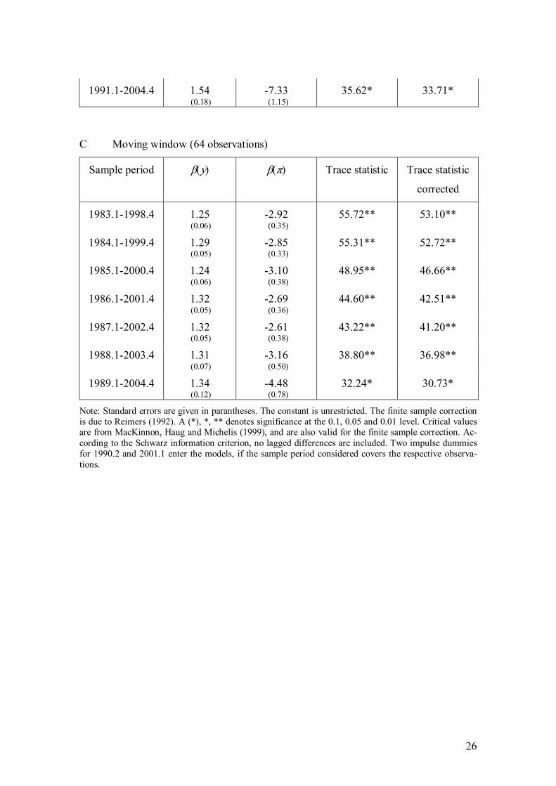
To gain insights into the stability of the cointegration property and the long run vector
in the (mp, y, π) system, recursive estimation techniques are applied. Table 2 exhibits
the results from this exercise, where the trace statistic and the cointegration vector are
estimated using forward and backward methods. Furthermore, the cointegration vector
is estimated by means of a moving window approach. Overall, the relationships seem to
be very stable, even in the pretented instability period after 2001. In particular, the coin
tegration finding can be confirmed in any case. There might be an upward shift in the
inflation coefficient in absolute value towards the end of the sample, but this change is
hardly significant.
Figure 3 and table 2 about here
5 Er ror correction modeling
Whether or not the cointegrating relationship can be interpreted in terms of a money
demand function is inferred from the error correction model. However, as we are mostly
interested in the stability of a money demand equation, the analysis is concentrated on
conditional single equation models (Johansen, 1995). A conditional model may lead to
constant coefficients even if a shift is present in the reduced form. Given the identifica
tion problems in full systems, a structural model for an individual variable might be
easier to develop using the single equation context.
At the initial stage of the estimation process, the contemporaneous and the first two lags
of the changes of all variables, a constant and the two impulse dummies are considered
in addition to the error correction term. It is also examined whether the dynamics are

11
affected by wealth effects, arising from the stock and housing markets (e.g. Kontolemis,
2002). In the first round, these variables could control for possible short run instabilities
in money demand. Then, the variables with the lowest and insignificant tvalues have
been eliminated subsequently (0.1 level). The final money demand relationship is (t
values in parantheses)
1 ( 1.60) ( 2.86) (7.11) (6.73) ( 5.13)
1 1 2 ( 2.58) (2.83) (1.92)
(4) ( ) 0.007 0.023 0.033 902 0.032 011 0.218 ( )
ˆ 0.113 ( ) 0.208 ( ) 0.140 ( )
t t t
t t t t
m p ec d d
m p m p u
π
π
− − − −
− − − −
∆ − = − − + + − ∆
− ∆ + ∆ − + ∆ − +
T=88 (1983.12004.4).
According to the negative coefficient of the error correction term ec, excess money low
ers money growth, as one expects in a stable model. In addition, changes in inflation are
significant. The results point to substantial inertia in the adjustment of real money bal
ances, as the feedback coefficient is very low and two lagged changes of money demand
are relevant in the specification. Finally, as the tvalues indicate, the impulse dummies
d902 and d011 should enter this equation.
Figure 4 and table 3 about here
Standard specification tests are largely supportive for the model, see the upper part of
table 3. LM is a Lagrange Multiplier test for autocorrelation in the residuals up to order
1, 4 and 8. The pvalues show, that no problems with autocorrelated residuals occur.
ARCH is a Lagrange multiplier test for conditional heteroskedasticity. Again, the re

12
siduals do not exhibit such kind of behaviour. Furthermore, they are distributed as nor
mal, as indicated by the JarqueBera test. The cusum of squares test does not indicate
any structural break in the regression coefficients, see the upper panel of figure 4. How
ever, the Ramsey RESET test points to a misspecification of the equation, as the third
order power of the fitted endogenous variable is significant at the 0.05 level. Nonlineari
ties in the relationship might account for this result. In fact, Carstensen (2004) and sev
eral other autors (e.g. Chen and Wu, 2005 for the US and the UK) have emphasized the
presence of nonlinearities in money demand behaviour. Lütkepohl, Teräsvirta and
Wolters (1999) have also detected nonlinearities in the development of the German M1
aggregate.
Due to the finding of the Ramsey test, a nonlinear analysis along the smooth transition
regression (STR) techniques as proposed by Granger and Teräsvirta (1993) and Teräs
virta (2004) has been carried out. However, the null of linearity cannot be rejected. The
results are omitted here to save space but are available from the authors upon request.
Compared to STR alternatives, the linear model is the superior choice.
Another modification of the basic equation (4) is able to overcome the problem. In par
ticular, a threshold autoregressive (TAR) specification of the error correction behaviour
which leads to an asymmetric adjustment process might be appropriate. In particular,
the existence of a monetary target can affect money demand. If money growth is above
its reference value, agents might reduce the demand for real money balances, as they
expect a rise in future inflation and a more restrictive monetary policy. To check the
robustness of the results, two models with different thresholds are estimated to investi
gate the TAR hypothesis.

13
The first choice for the threshold is related to the monetary target. Nominal money
growth in the euro area should be around 4.5 percent per annum. A dummy (tar1) is
introduced which is equal to 1 if actual growth is above the reference value and 0 oth
erwise. In most cases, nominal money growth exceeded this threshold, except of the
19941998 subperiod.
1 1 ( 2.57) ( 4.04) ( 3.71) (7.18)
1 1 (6.37) ( 5.49) ( 1.78) (2.19)
(5) ( ) 0.012 0.037 1 0.030 (1 1 ) 0.033 902
ˆ 0.030 011 0.231 ( ) 0.074 ( ) 0.165 ( )
t t t t t
t t t t
m p ec tar ec tar d
d m p u π π
− − − − −
− − − −
∆ − = − − − − +
+ − ∆ − ∆ + ∆ − +
T=88 (1983.12004.4)
The inclusion of the monetary target affects the speed of adjustment, see equation (5), as
the feedback coefficient is significantly larger (Wald test pvalue 0.0098) in absolute
value in periods of faster money growth than in periods of low money growth. Accord
ing to the evaluation tests, the specification of the equation has been improved (table 3,
figure 4). However, there are now some problems with higher order autocorrelation, and
the Ramsey statistic of order 2 is not far away from the critical 10 percent value. Thus, a
second choice for the threshold is considered (tar2). It refers to the sign of the mean
adjusted error correction term and is equal to 1 if the real money stock in the period
before the adjustment occurs is above its equilibrium and 0 otherwise.
1 2 ( 3.36) ( 4.97) ( 4.74) (6.94)
1 (6.93) ( 5.00) (3.45)
(6) ( ) 0.015 0.042 2 0.036 (1 2 ) 0.032 902
ˆ 0.033 011 0.206 ( ) 0.253 ( )
t t t t t
t t t
m p ec tar ec tar d
d m p u π
− − − − −
− −
∆ − = − − − − +
+ − ∆ + ∆ − +
T=88 (1983.12004.4)

14
This final equation survives all the tests, see the lower parts of table 3 and figure 4. Es
pecially, the pvalue for RESET(2) has further improved. In addition, the dynamic struc
ture has simplified. As in the previous model (5), the speed of adjustment is affected by
the monetary evolution. Again the feedback coefficient in absolute value is significantly
larger (pvalue 0.0051) for a positive deviation from equilibrium than for a negative
deviation. If either nominal money growth is above the reference value or the real
money stock exceeds its equilibrium, agents expect a rise in future inflation. Hence, the
opportunity costs of holding money will increase, thereby lowering money demand.
Overall, the empirical evidence in favour of a stable money demand equation for the
euro area is strongly supported by the error correction analysis.
6 Conclusion
In this paper we have analysed money demand behaviour in the euro area, where special
emphasis is given to the issue of stability. In fact, many researchers have detected insta
bilities especially when data after 2001 are included in the analysis. Such a result casts
serious doubts concerning the rationale of monetary aggregates in the monetary strategy
of the ECB. In contrast to the bulk of the literature, we report strong evidence in favour
of a stable money demand relationship. This result can be achieved by including infla
tion in the cointegration vector. If the analysis is done in this way a short run homoge
neity restriction between money and prices is not imposed. A long run money demand
relationship is identified, where recursive estimation lead to stable long run parameters.
In addition, the corresponding error correction model is robust to a wide range of speci
fication tests. Furthermore, the possibility of asymmetric adjustment by the inclusion of

15
a TAR specification of the error correction process improves the empirical fit of the
equation. In particular, the speed of adjustment is higher in periods of fast nominal
money growth and/or when the real money stock exceeds its equilibrium value, as the
agents expect a rise in future inflation. Therefore, the apparent monetary overhang is in
line with standard models of money demand behaviour, and can be rationalized by the
low opportunity costs of holding money.
16
References
Artis, M., Beyer, A. (2004): Issues in money demand. The case of Europe, Journal of
Common Market Studies 42, 717736.
Bosker, E.M. (2006): On the aggregation of eurozone data, Economics Letters 90, 260
265.
Brand, C., Cassola, N. (2004): A money demand system for euro area M3, Applied
Economics 8, 817838.
Brüggemann, R., Lütkepohl, H. (2005): A small monetary system for the euro area
based on German data, Journal of Applied Econometrics, forthcoming.
Bruggemann, A. P. Donati and A. Warne (2003), Is the Demand for Euro Area M3 Sta
ble?, in Issing, O. (ed.): Background Studies for the ECB’s Evaluation of Monetary Pol
icy Strategy, ECB Frankfurt, 245300.
Carstensen, K. (2004): Is European money demand still stable?, Kiel Institute of World
Economics, Working Paper 1179.
Chen, S.L., Wu, J.L. (2005): Long run money demand revisited: Evidence from a
nonlinear approach; Journal of International Money and Finance 24, 1937.
Coenen, G., Vega, J.L. (2001): The demand for M3 in the euro area, Journal of Applied
Econometrics 16, 727748.
Ericsson, NR. (1998): Empirical modelling of money demand, Empirical Economics 23,
295315.
European Central Bank (2003): Editorial, Monthly Bulletin, May, 58.

17
European Central Bank (2004): The monetary policy of the ECB.
Fagan, G., Henry, J. (1998): Long run money demand in the EU: Evidence for area
wide aggregates, Empirical Economics 23, 483506.
Funke, M. (2001): Money demand in Euroland, Journal of International Money and
Finance 20, 701713.
Gerlach (2004): The two pillars of the European Central Bank, Economic Policy 19,
389439.
Gerlach, S., Svensson, L. O. E. (2003): Money and Inflation in the Euro Area: a Case
for Monetary Indicators?, Journal of Monetary Economics 50, 164972.
Golinelli, R., Pastorello, S. (2002): Modelling the demand for M3 in the Euro Area.
European Journal of Finance 8, 371401.
Granger, C.W.J., Teräsvirta, T. (1993): Modeling nonlinear economic relationships,
Oxford University Press, Oxford.
Greiber, C., Lemke, W. (2005): Money demand and macroeconomic uncertainty, Deut
sche Bundesbank Discussion Paper 26/05.
Holtemöller, O. (2004a): Aggregation of national data and stability of euro area money
demand, in Dreger, C., Hansen, G. (eds): Advances in macroeconometric modelling.
Papers and Proceedings of the 3rd IWH Workshop in Macroeconometrics, Nomos, Ba
denBaden, 181203.
Holtemöller, O. (2004b), A monetary vector error correction model of the euro area and
implications for monetary policy, Empirical Economics 29, 553574.

18
Hubrich, K. (2001): Cointegration analysis in a German monetary system, Physica,
Heidelberg.
Hwang, H.S. (1985): Test of the adjustment process and linear homogeneity in a stock
adjustment model of money demand, Review of Economics and Statistics 67, 689692.
Johansen, S. (1995): Likelihood based inference in cointegrated vector autoregressive
models, Oxford University Press, Oxford.
Kontolemis, Z.G. (2002): Money demand in the euro area. Where do we stand?, IMF
Working Paper WP 02/185.
Lütkepohl, H., Teräsvirta, T., Wolters, J. (1999): Investigating stability and linearity of
a German M1 money demand function, Journal of Applied Econometrics 14, 511525.
Lütkepohl, H., Wolters, J. (2003): Transmission of German monetary policy in the pre
euro period, Macroeconomic Dynamics 7, 711733.
MacKinnon, G., Haug, A., Michelis, L. (1999): Numerical distribution functions of like
lihood ratio tests for cointegration, Journal of Applied Econometrics 14, 563577.
Neumann, M.J.M., Greiber, K. (2004): Inflation and core money growth in the euro
area, Deutsche Bundesbank Discussion Paper 36/04.
Reimers, H.E. (1992): Comparisons of tests for multivariate cointegration, Statistical
Papers 33, 335359.
Teräsvirta, T. (2004): Smooth transition regression modeling, in Lütkepohl, H., Krätzig,
M. (eds.): Applied time series econometrics, Cambridge University Press, Cambridge,
UK, 222242.

19
Wolters, J., Lütkepohl, H. (1997): Die Geldnachfrage für M3: Neue Ergebnisse für das
vereinigte Deutschland, ifo Studien 43, 3554.
Wolters, J., Teräsvirta, T., Lütkepohl, H. (1998): Modeling the demand for M3 in the
Unified Germany, Review of Economics and Statistics 80, 399409.

20
Figure 1: Variables used in the empirical analysis (levels)
7.6
7.8
8.0
8.2
8.4
8.6
8.8
84 86 88 90 92 94 96 98 00 02 04
Real money balances
6.8
6.9
7.0
7.1
7.2
7.3
7.4
7.5
84 86 88 90 92 94 96 98 00 02 04
Real income
.00
.02
.04
.06
.08
.10
.12
84 86 88 90 92 94 96 98 00 02 04
Short terminterest rate
.02
.04
.06
.08
.10
.12
.14
84 86 88 90 92 94 96 98 00 02 04
Long terminterest rate
.04
.02
.00
.02
.04
.06
.08
.10
84 86 88 90 92 94 96 98 00 02 04
Inflation
Note: Sample period 1983.12004.4. Real money and real GDP in logarithms and deflated by the GDP deflator.

21
Figure 2: Variables used in the empirical analysis (first differences)
.01
.00
.01
.02
.03
.04
.05
84 86 88 90 92 94 96 98 00 02 04
Real moneybalances
.008
.004
.000
.004
.008
.012
.016
.020
.024
.028
84 86 88 90 92 94 96 98 00 02 04
Real income
.03
.02
.01
.00
.01
.02
84 86 88 90 92 94 96 98 00 02 04
Short terminterest rate
.012
.008
.004
.000
.004
.008
.012
84 86 88 90 92 94 96 98 00 02 04
Long terminterest rate
.04
.03
.02
.01
.00
.01
.02
.03
.04
84 86 88 90 92 94 96 98 00 02 04
Inflation
Note: Sample period 1983.12004.4. Real money and real GDP in logarithms and deflated by the GDP
deflator.

22
Figure 3: Meanadjusted deviations from the long run
.3
.2
.1
.0
.1
.2
.3
84 86 88 90 92 94 96 98 00 02 04
Note: Sample period 1983.12004.4. Long run estimated according to equation (3a).

23
Figure 4: Cusum of squares of the error correction models
top: equation (4), mid: equation (5), bottom: equation (6)
0.2
0.0
0.2
0.4
0.6
0.8
1.0
1.2
86 88 90 92 94 96 98 00 02 04
0.4
0.0
0.4
0.8
1.2
1.6
95 96 97 98 99 00 01 02 03 04
0.2
0.0
0.2
0.4
0.6
0.8
1.0
1.2
86 88 90 92 94 96 98 00 02 04
Note: Sample period 1983.12004.4. Dashed lines represent 0.05 significance levels.

24
Table 1: Cointegration tests for sample period 1983.12004.4
Johansen trace test Variables Deterministics Rank null
hypothesis Lag order
Finite sample
correction
mp, y con_u, dum 0 1
9.04 2.01 [n=1]
rl, π con_r 0 1
19.82(*) 4.40 [n=2]
18.92(*)
rs, π con_r 0 1
32.10** 4.82 [n=1]
31.37**
rl, rs con_r 0 1
17.35 4.23 [n=2]
rl, rs, π con_r 0 1 2
32.55(*) 17.06(*) 4.49 [n=2]
30.33 15.89
mp, y, π con_u, dum 0 1 2
50.03** 8.39 2.25 [n=1]
48.32**
mp, y, rl con_u, dum 0 1 2
19.12 5.68 1.35 [n=1]
mp, y, rs con_u, dum 0 1 2
25.57 10.78 0.03 [n=1]
mp, y, π, rs con_u, dum 0 1 2 3
67.56** 24.34 10.59 0.001 [n=1]
64.49**
Note: con_u, con_r = constant unrestricted, restricted, dum = impulse dummies for 1990.2 and 2001.1, respectively. The finite sample correction is due to Reimers (1992). A (*), *, ** denotes significance at the 0.1, 0.05 and 0.01 level. Critical values are from MacKinnon, Haug and Michelis (1999), and are also valid for the finite sample correction. The lag order of the VAR in levels is determined by the Schwarz criterion with maximum lag order 8, and indicated by the number in brackets below the test values. The AIC and HQ criteria also point to the same lag order in all cases.

25
Table 2: Estimated cointegration parameters and trace tests
A Forward recursive estimates
Sample period β(y) β(π) Trace statistic Trace statistic
corrected
1983.11998.4 1.25 (0.06)
2.92 (0.35)
55.72** 53.10**
1983.11999.4 1.26 (0.05)
2.90 (0.33)
60.32** 57.66**
1983.12000.4 1.20 (0.06)
3.29 (0.37)
57.97** 55.56**
1983.12001.4 1.29 (0.05)
2.80 (0.34)
55.91** 53.70**
1983.12002.4 1.32 (0.05)
2.89 (0.36)
54.47** 52.43**
1983.12003.4 1.30 (0.06)
3.67 (0.49)
52.53** 50.66**
1983.12004.4 1.24 (0.09)
5.16 (0.72)
50.03** 48.32**
B Backward recursive estimates
Sample period β(y) β(π) Trace statistic Trace statistic
corrected
1983.12004.4 1.24 (0.09)
5.16 (0.72)
50.03** 48.32**
1984.12004.4 1.28 (0.08)
5.02 (0.70)
46.21** 44.56**
1985.12004.4 1.30 (0.08)
4.67 (0.70)
42.76** 41.16**
1986.12004.4 1.33 (0.08)
4.61 (0.71)
40.46** 38.86**
1987.12004.4 1.28 (0.09)
4.59 (0.75)
38.08** 36.50**
1988.12004.4 1.30 (0.10)
4.27 (0.72)
36.21** 34.61*
1989.12004.4 1.34 (0.12)
4.48 (0.78)
32.24* 30.73*
1990.12004.4 1.44 (0.16)
5.95 (0.98)
33.59* 31.91*
26
1991.12004.4 1.54 (0.18)
7.33 (1.15)
35.62* 33.71*
C Moving window (64 observations)
Sample period β(y) β(π) Trace statistic Trace statistic
corrected
1983.11998.4 1.25 (0.06)
2.92 (0.35)
55.72** 53.10**
1984.11999.4 1.29 (0.05)
2.85 (0.33)
55.31** 52.72**
1985.12000.4 1.24 (0.06)
3.10 (0.38)
48.95** 46.66**
1986.12001.4 1.32 (0.05)
2.69 (0.36)
44.60** 42.51**
1987.12002.4 1.32 (0.05)
2.61 (0.38)
43.22** 41.20**
1988.12003.4 1.31 (0.07)
3.16 (0.50)
38.80** 36.98**
1989.12004.4 1.34 (0.12)
4.48 (0.78)
32.24* 30.73*
Note: Standard errors are given in parantheses. The constant is unrestricted. The finite sample correction is due to Reimers (1992). A (*), *, ** denotes significance at the 0.1, 0.05 and 0.01 level. Critical values are from MacKinnon, Haug and Michelis (1999), and are also valid for the finite sample correction. Ac cording to the Schwarz information criterion, no lagged differences are included. Two impulse dummies for 1990.2 and 2001.1 enter the models, if the sample period considered covers the respective observa tions.

27
Table 3: Standard specification tests of error correction models
top: equation (4), mid: equation (5), bottom equation (6)
R2=0.59 SE=0.0046 SC=7.62
JB=1.44 (0.49)
LM(1)=0.07 (0.79) LM(4)=1.77 (0.14) LM(8)=1.30 (0.26)
ARCH(1)=1.71 (0.19) ARCH(4)=1.26 (0.29) ARCH(8)=0.64(0.74)
RESET(1)=2.52 (0.12) RESET(2)=3.65 (0.03) RESET(3)=2.40(0.07)
R2=0.61 SE=0.0045 SC=7.66
JB=1.70 (0.43)
LM(1)=0.32 (0.57) LM(4)=1.74 (0.15) LM(8)=1.87 (0.08)
ARCH(1)=0.60 (0.44) ARCH(4)=0.78 (0.54) ARCH(8)=0.33(0.95)
RESET(1)=0.44 (0.51) RESET(2)=2.06 (0.13) RESET(3)=1.36 (0.26)
R2=0.60 SE=0.0046 SC=7.67
JB=1.86 (0.40)
LM(1)=0.02 (0.89) LM(4)=1.72 (0.15) LM(8)=1.48 (0.18)
ARCH(1)=0.58 (0.45) ARCH(4)=1.17 (0.33) ARCH(8)=0.53(0.83)
RESET(1)=1.50 (0.22) RESET(2)=1.57 (0.21) RESET(3)=1.04(0.38)
Note: Sample period 1983.12004.4. R2=R squared adjusted, SE=standard error of regression, SC= Schwarz criterion, JB=JarqueBera test, LM=Lagrange multiplier test for no autocorrelation in the residu als, ARCH=Lagrange multiplier test against conditional heteroscedasticity, RESET=Ramsey test, p values in parantheses.


![A When and How to Use Multi-Level Modelling · Models and modelling play a cornerstone role in the Model-Driven Engineering (MDE) development paradigm [V¨olter and Stahl 2006]. In](https://img.dokumen.tips/doc/110x75/5f57d97200b6f74c484b13c6/a-when-and-how-to-use-multi-level-models-and-modelling-play-a-cornerstone-role-in.jpg)