#1. Flood Frequency Analysis Exercise

(1) Assume the design discharge is 30,000 cfs and determine the return period of this annual

maximum discharge in the period 1900 to 1940, and in the period 1941-2010. What was the

annual probability, p, of having a flood discharge of at least 30,000 cfs flowing through Austin in

the Colorado River before 1940? After 1940?

Years with annual maximum discharge equaling or exceeding 30,000 cfs 1900-1940 Exceedence Interval Recurrence

Interval (years) 1900 1902 2

1902 1903 1

1903 1904 1

1904 1905 1

1905 1906 1

1906 1908 2

1908 1909 1

1909 1913 4

1913 1914 1

1914 1915 1

1915 1916 1

1916 1918 2

1918 1919 1

1919 1920 1

1920 1921 1

1921 1922 1

1922 1923 1

1923 1924 1

1924 1925 1

1925 1926 1

1926 1927 1

1927 1928 1

1928 1929 1

1929 1930 1

1930 1931 1

1931 1932 1

1932 1933 1

1933 1934 1

1934 1935 1

1935 1936 1

1936 1937 1

1937 1938 1

1938 1940 2

Average 1.21

� = 1.21�����

�� > �� =1

�

�� > �� =1

1.21

�� > �� = 0.83

Years with annual maximum discharge equaling or exceeding 30,000 cfs 1941-2010

Exceedence Interval

Recurrence Interval (years)

1941 1957 16

1957 1958 1

1958 1960 2

1960 1961 1

1961 1975 14

1975 1977 2

1977 1987 10

1987 1992 5

1992 1997 5

1997 1999 2

1999 2002 3

2002 2005 3

2005 2010 5

Average 5.31

� � 5.31���

� � � ��� �1

�

� � � ��� �1

5.31

� � � ��� � 0.19

(2) A plot of the flood discharges for the annual peak flows of the Colorado River at Austin

including all the data and the historical flood.

(3) A plot and a table of results for the frequency analysis for the Colorado River at Austin for

the period 1900 to 1940.

Computed Curve

Expected Probability

Percent Chance

Exceedance

Confidence Limits 0.05 0.95

Flow (cfs) Flow (cfs)

1,066,182.40 1,428,381.40 0.2 2,141,525.60 651,738.60

716,499.60 885,877.70 0.5 1,322,901.40 463,397.80

523,817.00 613,816.60 1 906,087.30 353,765.40

377,632.30 423,193.50 2 611,165.30 266,414.00

237,958.70 254,000.80 5 352,078.00 177,787.40

162,453.60 168,950.20 10 224,569.80 126,485.00

105,994.10 108,007.90 20 137,399.40 85,413.70

51,931.20 51,931.20 50 63,653.20 42,101.10

28,923.50 28,596.00 80 36,010.70 22,158.10

22,338.40 21,906.10 90 28,379.90 16,470.30

18,468.40 17,940.70 95 23,895.70 13,193.50

13,624.10 12,982.40 99 18,227.30 9,214.50

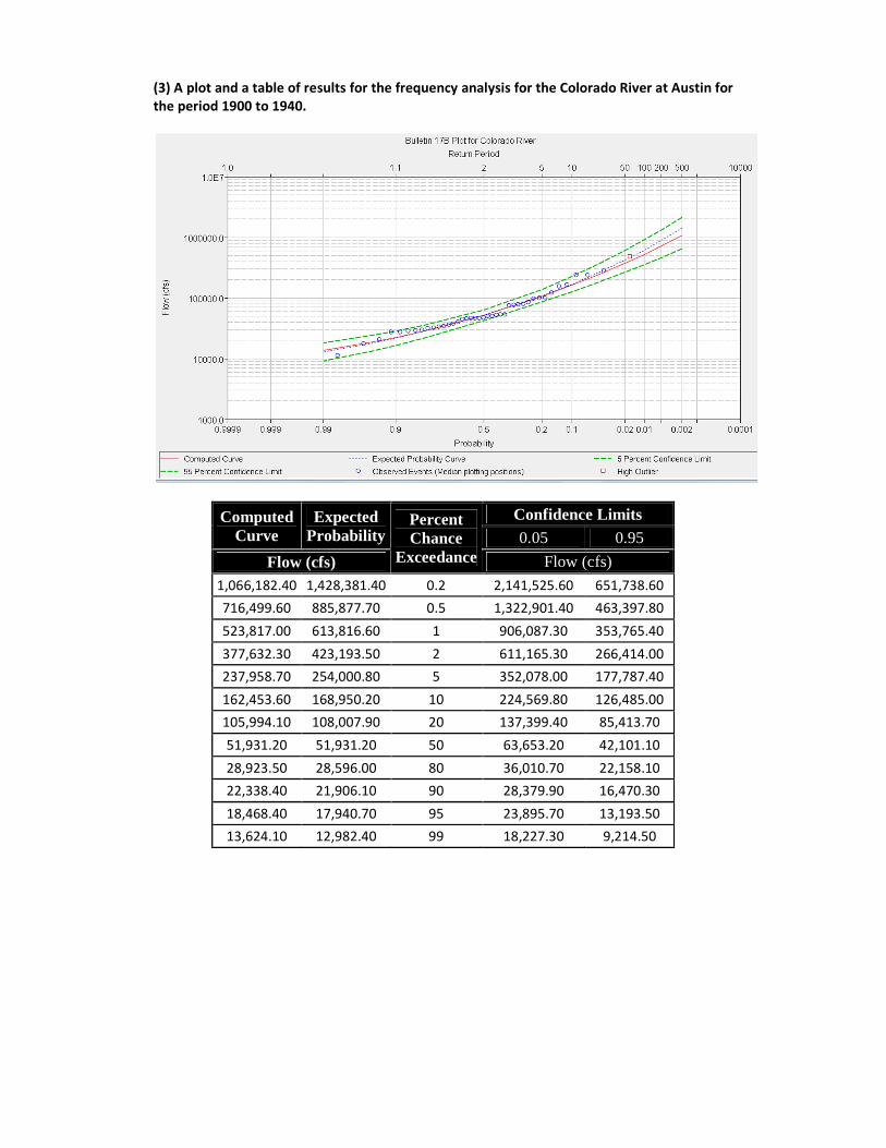
(4) A plot and a table of results for the frequency analysis for the Colorado River at Austin for

the period 1941 to 2010. Using the “Computed Curve Flows” make a comparison of the 2, 5,

10, 50 and 100 year design discharges for the two periods. By what amount did the

construction of the dams reduce the 100 year flood flow of the Colorado River at Austin?

What are the 95% confidence limits on the 100 year flood discharge estimate for the “After

Dams” condition?

Computed Curve

Expected Probability

Percent Chance

Exceedance

Confidence Limits 0.05 0.95

Flow (cfs) Flow (cfs)

127,143.80 141,741.30 0.2 193,368.70 91,919.20

97,256.90 105,519.80 0.5 142,135.30 72,391.40

78,196.30 83,293.10 1 110,703.40 59,562.20

61,802.30 64,776.30 2 84,618.60 48,218.80

43,684.70 44,962.80 5 57,068.30 35,229.80

32,288.30 32,873.90 10 40,624.90 26,711.30

22,558.70 22,766.80 20 27,320.90 19,111.70

11,619.50 11,619.50 50 13,539.10 9,963.90

6,161.40 6,111.10 80 7,277.30 5,081.70

4,473.30 4,405.10 90 5,396.30 3,566.30

3,454.10 3,372.00 95 4,256.40 2,668.10

2,156.70 2,054.40 99 2,779.30 1,563.30

Flow Before/After

Dams conditions

(%)

Percent

Chance

Exceedance

Return

Period

(years) 1900-1940 1941-2010

(cfs) (cfs)

523,817 78,196 15% 1 100

377,632 61,802 16% 2 50

267,286 47,756 18% 4 25

162,454 32,288 20% 10 10

105,994 22,559 21% 20 5

51,931 11,620 22% 50 2

The 100-year flood flow is reduced by:

523,817 − 78,196

445,621���

5% Confidence Limit: 110,703���

95% Confidence Limit: 59,562���

#2. 12.1.3 Calculate the probability that a 100-year flood will occur at a given site at least

once during the next 5, 10, 50 and 100 years. What is the chance that a 100-year flood will

not occur at this site during the next 100 years?

��� ≥ ��� = 1 − 1 −1

��

= 100�

� = 5, 10,50���100�

� ��� ≥ ���

5 0.05

10 0.10

50 0.39

100 0.63

What is the chance that a 100-year flood will not occur at this site during the next 100 years?

��� < ��� = 1 − ��� ≥ ���

��� < ��� = 1 − 0.63

��� < ��� = 0.37

#3. 12.5.1 Perform a frequency analysis for the annual maximum discharge of Walnut Creek

using the data given in Table 12.5.1, employing the log-Pearson Type III distribution without

the U.S. Water Resources Council corrections for skewness and outliers. Compare your

results with those given in Table 12.5.2 for the 2-, 5-, 10-, 25-,50- and 100-year events.

Year Flow (cfs) y=log(x) ��− ���� ��− ����

1967 303 2.4814 1.3395 -1.5502

1968 5,640 3.7513 0.0127 0.0014

1969 1,050 3.0212 0.3814 -0.2356

1970 6,020 3.7796 0.0198 0.0028

1971 3,740 3.5729 0.0043 -0.0003

1972 4,580 3.6609 0.0005 0.0000

1973 5,140 3.7110 0.0052 0.0004

1974 10,560 4.0237 0.1481 0.0570

1975 12,840 4.1086 0.2207 0.1037

1976 5,140 3.7110 0.0052 0.0004

1977 2,520 3.4014 0.0564 -0.0134

1978 1,730 3.2380 0.1606 -0.0644

1979 12,400 4.0934 0.2067 0.0940

1980 3,400 3.5315 0.0115 -0.0012

1981 14,300 4.1553 0.2668 0.1378

1982 9,540 3.9795 0.1161 0.0396

Total 58.2206 2.9555 -1.4280

n= 16

Sy= 0.4439

��= 3.6388

Cs= -1.2440

A B C D

Return Period

[yr]

Frequency factor

(��)

��=log(Qt) Qt [cfs]

2 0.202 3.7285 5,351

5 0.841 4.0121 10,282

10 1.076 4.1164 13,074

25 1.264 4.1999 15,844

50 1.355 4.2403 17,388

100 1.420 4.2691 18,583

Column B: Interpolating from Table 12.3.1

Column C: �� = �� + ����

Column D: �� = 10��

#4. 14.2.1 Determine the 10-year, 1-hour design rainfall intensity and depth for Chicago from

the IDF curve given in Fig. 14.2.1.

= 10�

� = 1ℎ = 60���

(Fig. 14.2.1)

� = 2.1��/ℎ

The results are similar for 2-, 5- and 10-year events. For the rest, the computed results are

almost significantly smaller.

#5. 14.5.1 Use Eq. (14.5.1) for the world’s greatest recorded rainfalls to develop and plot a

24-hour design hyetograph in 1-hour time increments by the alternating block method.

� = 422��.�

Duration Td

[hr]

Cumulative

Precipitation

[mm]

Incremental

Precipitation

[mm]

Precipitation

[mm]

1 422 422 39

2 587 165 41

3 711 125 43

4 815 104 46

5 906 91 49

6 988 82 53

7 1,063 75 58

8 1,133 70 65

9 1,198 65 75

10 1,260 61 91

11 1,318 58 125

12 1,374 56 422

13 1,427 53 165

14 1,478 51 104

15 1,527 49 82

16 1,575 48 70

17 1,621 46 61

18 1,666 45 56

19 1,709 43 51

20 1,751 42 48

21 1,792 41 45

22 1,832 40 42

23 1,871 39 40

24 1,909 38 38

0

50

100

150

200

250

300

350

400

450

1 2 3 4 5 6 7 8 9 10 11 12 13 14 15 16 17 18 19 20 21 22 23 24

Pre

cip

ita

tio

n [

mm

]

Time [hr]