1 Finding Similar Items

This chapter discusses the various measures of distance used to find out similarity betweenitems in a given set. After introducing the basic similarity measures, we look at how to dividea document into pieces called as k-shingles and use them to compare two documents. Next,the concept of min-hashing is introduced which provides a novel signature for the documents.Finally, we explore the topic of Locality Sensitive Hashing (LSH) which is a very neat method ofcomputing nearest neighbors in a much more computationally efficient manner. Needless to say,all these techniques discussed in this chapter find several applications in the real-world today dueto the massive explosion in the scale of data. Examples of modern day LSH applications includefingerprint matching, removing duplicate results from the search results page of search enginesand matching music tracks by looking at segments of them (eg: apps like Shazam, SoundHounduse related techniques to perform blazingly fast similarity matches in real-time).

1.1 Popular Measures of Similarity between items

In Recommender Systems, collaborative filtering is a widely used technique to recommend itemsto users that were liked by other users having similar interests. Suppose we wish to find outif two netflix users - Alice and Bob have the same movie viewing pattern. Given their watchhistory, which contains a set of movies they have watched in the past few months, if we cancompute some notion of how similar these two sets are, then that gives us a rough indication ofthe similarity between Alice and Bob. Although not the most efficient way to solve this problem,this is a good start.

Consider the following concrete example, where M1 and M2 are Alice’s and Bob’s viewing his-tory over the past month.M1 = {"ride along", "the hundred foot journey", "love is in the air", "it felt like love", "interstellar"},andM2 = {"interstellar", "big men", "tarzan", "into the storm", "the hundred foot journey"} .

The Jaccard Similarity of the sets M1 and M2 is given by |M1∩M2||M1∪M2| , that is, the fraction of the

elements which are common to both the sets given the total number of (combined) elements inthe two sets. In this example, the Jaccard Similarity between Alice and Bob would be 2

8 = 14 .

Jaccard Distance1 between M1 and M2 is then simply defined as 1− 14 = 3

4 .

Now, suppose we took the entire set of movies available on netflix, say a million of them andformed a million-dimensional euclidean space out of them (with each dimension representinga movie). Then Alice and Bob can be represented as two points in this euclidean space, wheretheir corresponding position vectors will have 1’s for the movie they watched recently and 0’severywhere else. The problem of finding similiarity between them boils down to computing the

1Although this section uses both the terms similarity and distance, they are just inverses of each other. For everysim(.) measure, the corresponding dist(.) measure can be expressed as 1− sim(.), provided the similarity measure isnormalized appropriately.

1

cosine similarity between their vectors m1 and m2, which is given by:

sim(m1, m2) = cos(m1, m2) =m1 ·m2

‖m1‖‖m2‖ (1)

Another way to measure the distance between the vectors m1 and m2, is to use the HammingDistance which is defined as the number of components in which the two vectors differ. In ourexample, the hamming distance between Alice and Bob would be 3 (as they differ in 3 moviesout of the 5 considered in the list).

Euclidean Distance is another widely used distance measure in such cases which is defined as:

d(m1, m2) =

√√√√ d

∑i=1

(m(i)1 −m(i)

2 )2 (2)

where, d is the number of components or dimensions of m1 and m2. Also known as the l2 normbetween the vectors m1 and m2, this measure is a special case of the general lp norm family. Thelp norm between two vectors is defined as:

d(m1, m2) = (d

∑i=1|m(i)

1 −m(i)2 |

p)

1p (3)

As can be seen, on setting p = 2 we obtain the Euclidean norm as a special case and settingp = 1 we obtain the l1 norm (also called the Manhattan Distance) between two vectors. In theextreme case, when p = ∞, we obtain the l∞ norm, which is defined as largest difference in thedimensions (as the other dimensions do not matter when p goes to ∞). ie,

l∞ = maxi|m(i)

1 −m(i)2 | (4)

Earlier in this section when we computed the Jaccard Similarity between the sets M1 and M2, wecounted an item to be in the intersection of both of them if had exactly the same movie name(ie, the movie strings matched textually). For example, both M1 and M2 had the movie "the hun-dred foot journey". However, if one of these movie names was stated in a different way or hadspelling errors such as "the hundred ft journey", the above method would not work. Thereforewe have to look for a way to match strings approximately tolerating all of these possibilities.Edit Distance is one such method that provides a measure of how far a source string is froma destination string by recording the number of character insertions, character deletions and/orcharacter substitutions that need to be made to convert the source string into the target string.In our case, the edit distance between the strings "the hundred foot journey" and "the hundred ftjourney" is equal to 2.

All the above measures we discussed above qualify to be a valid distance metric because they obeythe following properties:If x, y are two points and d(·) is the distance metric between them, then:

• distance is non-negative. ie, d(x, y) is always ≥ 0

2

• distance between similar points is zero. ie, d(x, y) = 0 if x = y

• distance is symmetric. ie, d(x, y) = d(y, x)

• distances obey the triangle inequality. ie, d(x, y) ≤ d(x, z) + d(z, y). What this essentiallymeans is that, when traveling from point x to y, there is really no benefit in traveling viasome particular third point z.

1.2 Shingles and Min-Hashing

Given that we discussed about measuring similarities between sets in the previous section, howdo we represent two documents in the form of sets so that we can use measures like Jaccard Sim-ilarity on them? One effective way to do this is by constructing a set of all k-length substringsout of a document called shingles of length-k or k-shingles. Note that each shingle could appearone or more times in the document. Shingles help in capturing the short portions of text thatare often shared across the documents. Lets look at a toy example. Suppose our document Dcontains the text "abcdabd", the set of all 2-shingles for D is {ab, bc, cd, da, bd}. Observe that whenthe document contains words delimited by spaces, depending on whether spaces are ignored ornot, different shingles would be produced. Also, the length of the shingle determines the levelof granularity desired in capturing the repetitive text across documents. What this means is that,with very low values of k (eg: say k=1), almost all documents will have common characters andhence all of them will have high similarity. On the contrary, if k is set to very large value, sayequal to average size of all the documents being compared, there is a chance that there is hardlyany repetitive segment found and hence all of the documents will have zero similarity. Thuschoosing the appropriate size for the k-shingle is important and two factors to be considered arehow long typically documents are and how large the typical set of characters is. A good rule ofthumb in general is: k should be picked large enough that the probability of any given shingle appearingin any given document is low.

A key question to ask now is how to represent and store these sets of shingles? Suppose wehave a corpus of email documents. Typically only letters and a general whitespace characterappear in emails, so the total number of shingles (assuming for instance that k=5) would be275 = 14, 348, 907 shingles. Such large number of shingles may sometimes not even fit in thememory and even if they did, the number of pairs to compare similarities for will be astron-ishingly large. We need to compress the shingles in such a way that also lets us compare themeasily. Fortunately, we can do this pretty effectively by representing these sets compactly intotheir signatures and then using the signatures to estimate similarities like Jaccard. The natureof these signatures is such that they do not guarantee exactly similarity of the sets they repre-sent, but provide very close estimates, and these estimates get better when have larger signatures.

This is great, but how do we compute these signatures efficiently? This can be achieved thanksto a neat technique called MinHashing. Lets look at an example to see what MinHash computes.

Going by the same example as earlier, suppose we have the data about the users on netflix

3

and what movies they watched recently. Let each movie m ∈ M be indexed by a unique id fromthe set {1 . . . M} and each user u ∈ U be indexed by an alphabet in the set {A . . . Z}. Clearly, agiven user is a set whose elements are equal to the movie-id’s he watched, and each user is thusa subset ofM. Now, consider the two sets (or users) A = {1, 2}, B = {2, 3}.

Steps to compute MinHash:

• Pick a permutation π of the setM uniformly at random.

• Hash each subset S ⊆ U to the minimum value it contains according to π

Assume that π = (2 < 1 < 3), then the minhash of A is computed as h(A) = 2, as 2 is theminimum value in the set A according to the ordering imposed by π. Likewise, h(B) = 2 aswell. Now, lets enumerate all the possible permutations along with their corresponding min-hashes for the sets A and B. That gives us the signature for all the set of users (or documents- if we are looking for similar text documents). This will also lead us to an interesting observation.

π = (1 < 2 < 3), h(A) = 1, h(B) = 2, π = (2 < 3 < 1), h(A) = 2, h(B) = 2π = (1 < 3 < 2), h(A) = 1, h(B) = 3, π = (3 < 1 < 2), h(A) = 1, h(B) = 3π = (2 < 1 < 3), h(A) = 2, h(B) = 2, π = (3 < 2 < 1), h(A) = 2, h(B) = 3

Shown here are all the possible 6 permutations for the set U . The minhashes of the sets Aand B are equal for 2 out of 6 permutations, (ie: 1

3 times); but more importantly observe that thisfraction 1

3 is actually equal to the Jaccard Similarity between the sets A and B.

In other words, the probability that the minhash function h(·) for a random permutation π producesthe same value for two sets A and B equals the Jaccard Similarity between the sets A and B. This isa remarkable connection. What this means is that minhashes can be used to calculate JaccardSimilarities in a much more quick and space-efficient manner.

Creating the compact signatures for the documents (or, users in this example) is now easy. Wecan think of the each movie m ∈ M as a row of a matrix (we call this the signature matrix) andeach user u ∈ U as a column. In our original representation, each column would thus have avalue (say 0 or 1) against the relevant row, but in the signature representation we replace thesewith the minhash value corresponding to the user and the permutation. Note that we haveshrunk M rows of binary values to just one row of minhashes for that permutation. Computingthe minhashes for say a 100 permutations, we obtain our final signature matrix composed ofseveral rows of minhashes. It should be noted that however, the minhash functions used for eachrow could all be different (ie. h1(), h2(), ..). It is easy to see that the signature matrix has size(100×U ) much smaller than the original matrix (M×U ).

In reality, computing the permutations of the rows from theM×U matrix can be very expensive.Even picking a random permutation from millions of rows could be time-consuming. Thus, hashfunctions are used as technique to simulate the effect of a random permutation of the rows. Thesefunctions map the row numbers to as many buckets as there are rows. There is a small chance

4

that one of these functions might map two different rows to the same bucket; however in practiceoften number of rows is so large that these minimal collisions do not matter. In summary, insteadof picking n permutations of the rows, n randomly chosen hash functions h1(), h2(), · · · hn() arepicked to operate on the rows. Rest of the process of constructing the signature matrix remainsthe same as discussed previously.

1.3 Locality Sensitive Hashing (LSH)

Although the technique of minhashing helps us compute signatures effectively and computesimilarity of pairs of documents quickly, it does not alleviate the task of considering all possi-ble pairs. If we have a million documents and use signatures of length 250, even if takes just amicro-second to compute the similarity of two signatures, we might still spend around 6 dayscomputing the similarities across all pairs of documents. Therefore we want to avoid looking at allexisting pairs and focus only on those which have very high probability of being similar. Locality-SensitiveHashing (LSH) provides a theory for how to choose such important pairs. In many real-world use-cases,the saving in terms of computation and time obtained by using these techniques is massive.

LSHs represent similarities between objects using probability distributions over hash functionsand operate on the key idea that Hash collisions capture object similarity.

1.3.1 LSH: Gap Definition

The original definition of LSH (also called the Gap Definition) states the following. Consider asimilarity function over a universe U of objects, S : U × U → [0, 1]. An (r, R, p, P)-LSH for asimilarity S is a probability distribution defined over a set H of hash functions such that:

• S(A, B) ≥ R⇒ Prh∈H[h(A) = h(B)] > P

• S(A, B) < r ⇒ Prh∈H[h(A) = h(B)] < p

for each A, B ∈ U. Also, r < R and p < P.

What this means is that - if the similarity between objects A and B is at least R, then the probability thattheir hashes collide (or are the same) is atleast P. Likewise, if the similarity between A and B is atmost r,then the probability that their hashes will be the same is atmost p. Note that there is a gap between Rand r, and between P and p; hence the name Gap Definition.

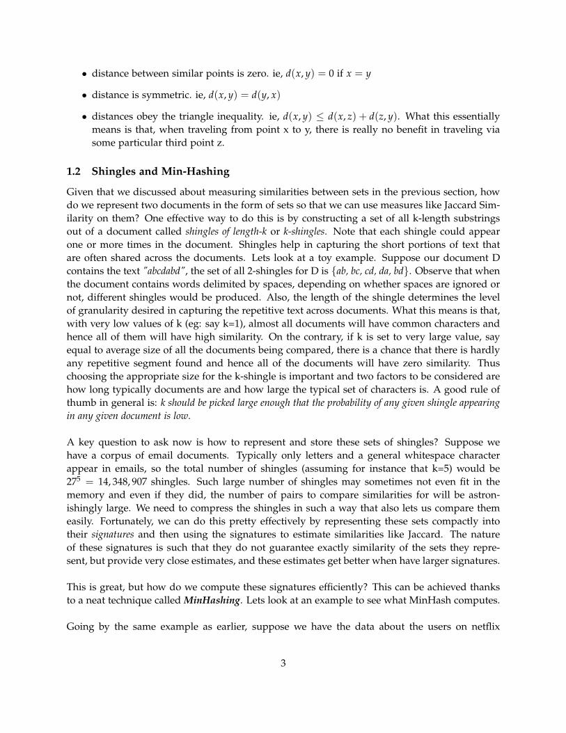
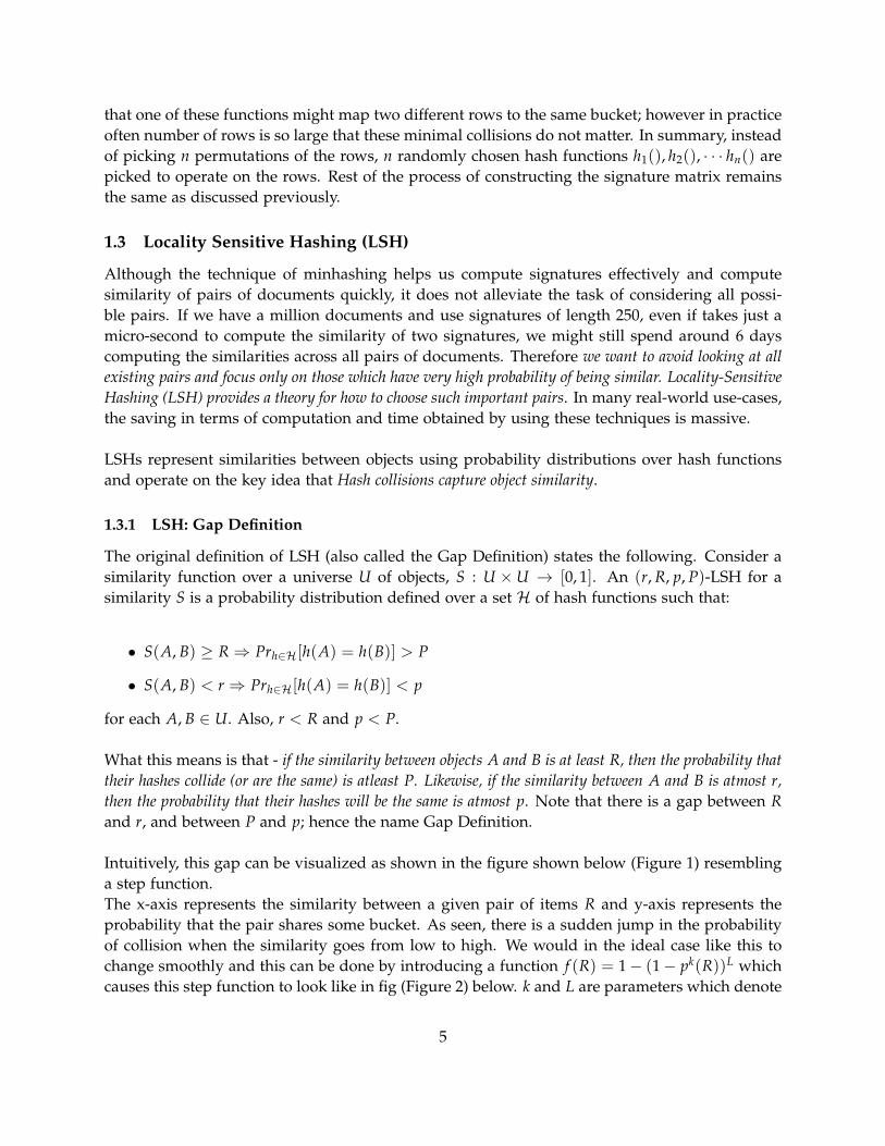
Intuitively, this gap can be visualized as shown in the figure shown below (Figure 1) resemblinga step function.The x-axis represents the similarity between a given pair of items R and y-axis represents theprobability that the pair shares some bucket. As seen, there is a sudden jump in the probabilityof collision when the similarity goes from low to high. We would in the ideal case like this tochange smoothly and this can be done by introducing a function f (R) = 1− (1− pk(R))L whichcauses this step function to look like in fig (Figure 2) below. k and L are parameters which denote

5

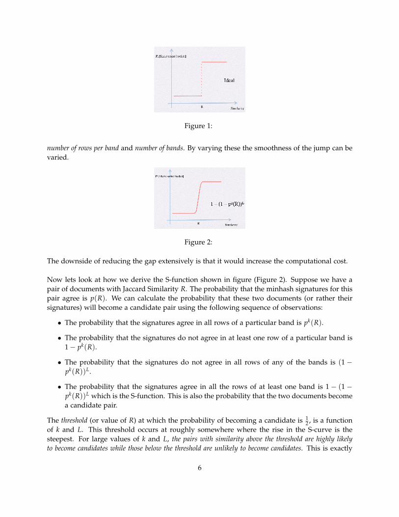
Figure 1:

number of rows per band and number of bands. By varying these the smoothness of the jump can bevaried.

Figure 2:

The downside of reducing the gap extensively is that it would increase the computational cost.

Now lets look at how we derive the S-function shown in figure (Figure 2). Suppose we have apair of documents with Jaccard Similarity R. The probability that the minhash signatures for thispair agree is p(R). We can calculate the probability that these two documents (or rather theirsignatures) will become a candidate pair using the following sequence of observations:

• The probability that the signatures agree in all rows of a particular band is pk(R).

• The probability that the signatures do not agree in at least one row of a particular band is1− pk(R).

• The probability that the signatures do not agree in all rows of any of the bands is (1−pk(R))L.

• The probability that the signatures agree in all the rows of at least one band is 1− (1−pk(R))L which is the S-function. This is also the probability that the two documents becomea candidate pair.

The threshold (or value of R) at which the probability of becoming a candidate is 12 , is a function

of k and L. This threshold occurs at roughly somewhere where the rise in the S-curve is thesteepest. For large values of k and L, the pairs with similarity above the threshold are highly likelyto become candidates while those below the threshold are unlikely to become candidates. This is exactly

6

the ideal behavior we want. For most practical purposes, ( 1L )

1k is a good approximation of this

optimal value for the threshold.

Below is an algorithm that uses LSH to find documents that are truly similar.

Algorithm

1: Choose a value of k and construct a set of k-shingles from the documents. An alternateis to hash the k-shingles to shorter bucket numbers to make it more efficient.

2: Sort the document-shingle pairs to order them by shingle.3: Pick a length n for the minhash signatures. Compute the minhash signatures for all the

documents.4: Choose a threshold t that decides how similar documents have to be in order for them to

be regarded as a desired similar pair.5: Divide n into multiple bands L each of size k rows. Calculate the threshold t as ( 1

L )1k .

The choice of L and k also controls the number of false positives and false negatives.Depending on whether the priority is to avoid false negatives or false positives, the valuesof b and r need to be chosen to produce a threshold lower or higher than t respectively.

6: Construct candidate pairs by applying the LSH technique described earlier.7: Examine each candidate pair’s signatures and determine whether the fraction of compo-

nents in which they agree is at least t.8: Optionally, if the signatures are sufficiently similar, go to the documents themselves and

check that they are indeed similar, rather than documents that, by luck, had similarsignatures.

1.3.2 Constructing LSH families for common distance measures

We saw earlier that for a similarity metric (or equivalently every distance measure) to have anLSH, the gap definition needs to be satisfied. Lets see how we can find LSH’s for some commonlyused distance measures and the rationale behind them.

• Hamming SimilarityLet HS(x, y) denote the Hamming Similarity between x and y. We then define SamplingHash as H = {h1, .., hn}, where hi(x) = xi (ie. the i-th hash function outputs the i-th bitof x). It is easy to see that this hash function forms an LSH for the Hamming Similaritybecause:

Pr[h(x) = h(y)] = Pri[hi(x) = hi(y)] = HS(x, y) (5)

• Jaccard SimilarityLet JS(x, y) denote the Jaccard Similarity between x and y. If we define a MinHash as we

7

discussed in section (reference section), then clearly this hash function forms an LSH forthe Jaccard Similarity because:

Pr[h(A) = h(B)] =|A ∩ B||A ∪ B| = J(A, B) (6)

This can also be easily verified using the fig below (Figure 3).

Figure 3:

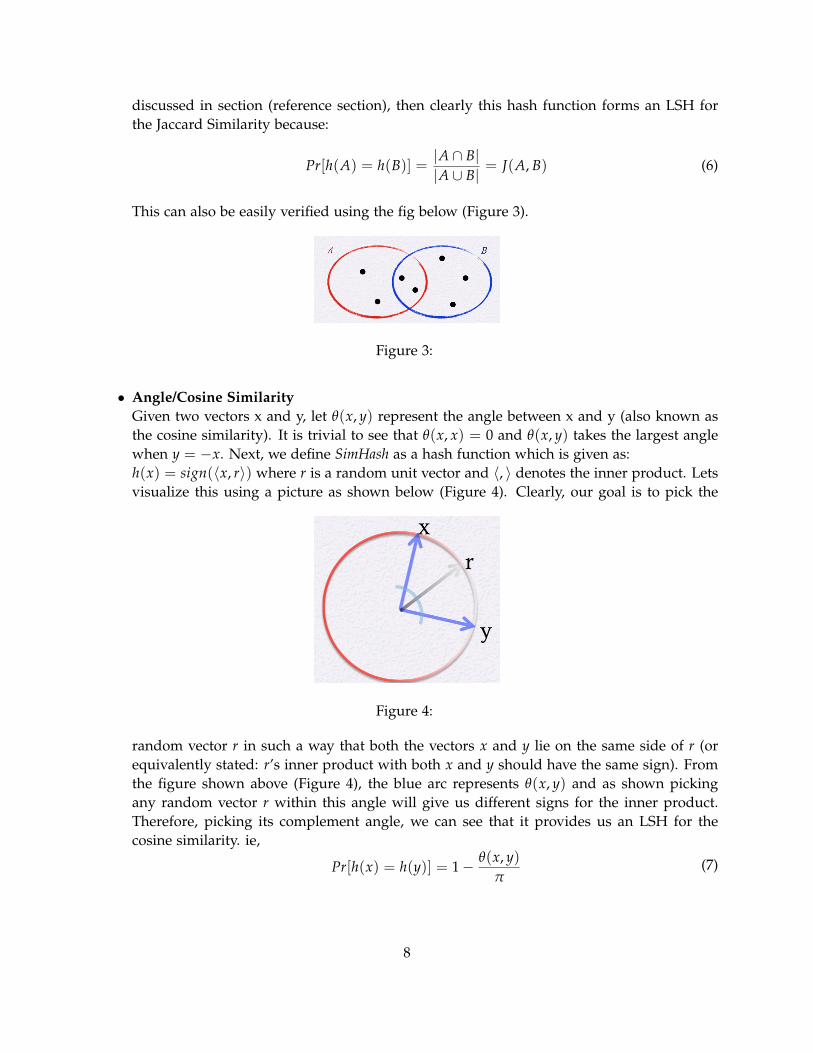
• Angle/Cosine SimilarityGiven two vectors x and y, let θ(x, y) represent the angle between x and y (also known asthe cosine similarity). It is trivial to see that θ(x, x) = 0 and θ(x, y) takes the largest anglewhen y = −x. Next, we define SimHash as a hash function which is given as:h(x) = sign(〈x, r〉) where r is a random unit vector and 〈, 〉 denotes the inner product. Letsvisualize this using a picture as shown below (Figure 4). Clearly, our goal is to pick the

Figure 4:

random vector r in such a way that both the vectors x and y lie on the same side of r (orequivalently stated: r’s inner product with both x and y should have the same sign). Fromthe figure shown above (Figure 4), the blue arc represents θ(x, y) and as shown pickingany random vector r within this angle will give us different signs for the inner product.Therefore, picking its complement angle, we can see that it provides us an LSH for thecosine similarity. ie,

Pr[h(x) = h(y)] = 1− θ(x, y)π

(7)

8

1.4 Applications

• Entity ResolutionEntity Resolution is the problem of finding whether two user records (such as mailingaddresses of restaurants in a city) are the same or not. For simplicity lets assume the recordconsists of three fields only - name, street, phone. This is an essential problem to solve in reallife applications where the records come from diverse data sources and each data sourcescould have encoded the address in different ways, with spelling errors and other missinginformation (such as zip code being absent, etc). A simple strategy that would work isto score a pair based on difference in the available fields. However, when we have largenumber of records, it is not feasible to score every possible pair (this number could rise upto a trillion for example) and hence we need an LSH to focus on the most likely candidates.How could we generate one? We use "three" hash functions for this purpose. The first onehashes the records based on the name field, second one based on the street field and thirdone based on the phone field. A clever trick can help us avoid computing these hashes. First,we sort the records based on name field; this would cause all records with identical namesto appear consecutively and get scored for overall similarity of name, street and phone.Next, we apply another sorting based on the street field; the records get sorted by streetand those with same street are scored. Finally, the records are sorted by phone field andthe records with identical phones are scored.

• Fingerprint MatchingUnlike many other identity matching applications, fingerprints are not matched by theirimage; instead a set of locations in each fingerprint which determine the uniqueness of thefingerprint (termed as minutiae) are identified and two fingerprints are matched by check-ing if a set of grid squares contains these minutiae in both the fingerprints. Typically wehave two use-cases:- many-one problem: This is the case when a fingerprint has been found on a gun and wewish to compare it with all the fingerprints in a large database. This is the more commonscenario.- many-many problem: In this case, we take the entire database and check if there are anypairs which represent the same individual. For instance, taking the first page of googlesearch results and identifying if there are any pairs representing the same result.

Lets look at how we can make these comparisons faster using a variant of LSH that suitsthis problem. Suppose the probability of finding a minutia in a random grid square ofa random fingerprint is 20%. Next, assume that if two fingerprints come from the samefinger and one has a minutia in a given grid square, then the probability that the other doestoo is 80%. We propose a LSH family of hash functions F in the following manner. Eachf ∈ F is defined as below (using a context of three specific grid squares):f (x, y) = yes, if two fingerprints x & y have minutiae in all three grid squares,f (x, y) = no, otherwise.Another interpretation of the function f is that f sends to a single bucket all fingerprintsthat have minutiae in all three grid squares, and sends each other fingerprint to a bucket of

9

its own.

How to solve the many-one problem using this LSH? Invoking several functions from the familyF we precompute their buckets of fingerprints to which they answer "yes". Then, givena fingerprint under investigation, we determine which of these buckets it belongs to andcompare it with all the fingerprints found in any of those buckets.

How to solve the many-many problem using this LSH? We compute the buckets for each ofthese functions and compare all fingerprints in each of the buckets.

Analysis: How many functions do we need to achieve a reasonable probability of detecting amatch? (without of course, having to compare the fingerprint on the gun with the millionsof fingerprints in the database) Observe that, the probability that two fingerprints fromdifferent fingers would be in the same bucket for a function f ∈ F is (0.2)6 = 0.000064.These two fingerprints would go into the same bucket if they each have a minutia in eachof the three grid squares associated with f . Now, lets consider the probability that twofingerprints from the same finger end up in the bucket for f . Probabiliy that the first fin-gerprint has minutiae in each of the three grid squares belonging to f is (0.2)3 = 0.008.Then, the probability that the other fingerprint also has minutiae in the same grid squaresis (0.8)3 = 0.512. Hence, if the two fingerprints are from the same finger, then there is aprobabiliy of 0.008× 0.512 = 0.004096 that they will both be in the bucket of f . Noticethat this is not a big number, but if we make use of many more functions from the familyF , then we can arrive at a reasonable probability of matching fingerprints from the samefinger. We also will be able to avoid having too many false positives.

1.5 Methods for High Degrees of Similarity

LSH based methods are very effective when the degree of similarity we want to accept is rela-tively low. However, there are use cases where we would want to find pairs which are almostidentical and in such cases, there are other methods that are much faster. Since these methodsare based on exact similarity, there are no false negatives as in the case of LSH.

• Finding Identical ItemsAssume for example that we need to find web-pages which are identical exactly, ie, character-by-character. Our goal is to avoid comparing every pair of documents. The first idea couldbe to hash documents based on either the first few characters of the document or the entiredocument itself. However, documents often have the same HTML header in which case theformer fails and the later approach has a downside that we need to look at every characterin the document to compute the hash, which could be expensive. An alternative approachwould be to pick certain random locations in the document and compute hashes at thosesegments. If the documents are indeed similar, then such a hash function would returnexactly the same value. Also, we do not need to consider documents of varying lengthanyways.

• Length-Based Filtering

10

Lets look at a more harder problem of finding from a huge collection of sets, all the pairshaving a high Jaccard Similarity, say at least 0.9. We represent a set by sorting the elementsof the universal set in some fixed order, and representing any set by listing its elements inthis order. For instance, if the universal set contains the 26 lower-case letters and we usethe normal alphabetical order; then, the set {d, a, b} is represented by the string abd.

Now, lets look at how we can exploit this construction. The simplest way is to sort thestrings by length. Then, each string s is compared with those strings t that follow s in thelist, but are not too long. Suppose there exists an upper bound J on the Jaccard Distancebetween two strings. Let Lx denote the length of a string x. Note that Lx ≤ Lt. The intersec-tion of the sets represented by s and t cannot have more than Ls elements, while their unionwill have at least Lt elements. Therefore, the Jaccard Similarity of s and t, JS(s, t) ≤ Ls

Lt. This

means in order for s and t to require comparison, it must be that J ≤ LsLt

, or equivalently,Lt ≤ Ls

J . This gives us an estimate of the length of the candidate strings t that we need toconsider to compare s with in order to achieve our desired Jaccard Similarity.

• Prefix IndexingRetaining the same construction as above, lets look at other features of strings that can beexploited to reduce the number of pairwise comparisons. One such method is to createan index for each symbol from our universal set. For each string s, we select a prefix of sconsisting of the first p symbols of s. How large p must be depends on Ls and J (definedin the method in previous paragraph). We add string s to the index for each of its first psymbols.

The index for each symbol becomes a bucket of strings that must be compared. We needto be certain that any other string t such as JS(s, t) ≥ J will have at least one symbol in itsprefix that also appears in the prefix of s.However, if JS(s, t) ≥ J, but t has none of the firstp symbols of s. Then the higest Jaccard Similarity that s and t can have occurs when t isa suffix of s, consisting of everything but the first p symbols of s. The JS of s and t wouldthen be (Ls−p)

Ls. In order to be sure that we do not have to compare s with t, we must be

certain that J > (Ls−p)Ls

. ie, p ≥ b(1− J)Lsc + 1. Note that, we want p to be as small aspossible, so that we do not index the string s in more buckets than we need to. Thus, wetake p = b(1− J)Lsc+ 1 as length of the prefix to be indexed.

• Using Position and Suffix IndexesLike the above methods, we can also index strings by the position of that character withinthe prefix as well as the length of the characterâAZs suffix âAS the number of positions thatfollow it in the string. In the former case, we can reduce the number of pairs of strings thatmust be compared, because if two strings share a character that is not in the first positionin both strings, then we know that either there are some preceding characters that are inthe union but not the intersection, or there is an earlier symbol that appears in both strings.The later case reduces the number of pairs that must be compared, because a commonsymbol with different suffix lengths implies additional characters that must be in the union

11

but not in the intersection.

1.6 Acknowledgements

This document is a compressed version of Chapter: 3 "Finding Similar Items" from the book "Min-ing of Massive Datasets" by Jure Leskovec, Anand Rajaraman and Jeffrey D. Ullman. While most partsof this document are directly based on this chapter, some have been re-written from scratch.Another source of inspiration for this document is the talk by Ravi Kumar (Google) on LSH atMachine Learning Summer School (MLSS 2012), UC Santa Cruz. Some of the material in Section 1.3(including the figures) are derived from slides based on this talk.

12