1

Experimental StatisticsExperimental Statistics - week 3 - week 3Experimental StatisticsExperimental Statistics - week 3 - week 3

• Statistical Inference2-sample Hypothesis Tests

Review ContinuedReview Continued

Chapter 8: Inferences about More Than 2 Population Central Values

2

Note:Thursday we will have class in the computer lab (Room 15 Clements - basement. Enter from North side, west stairs.)

I suggest that you download the file “car.dat” from my internet site onto a 3 1/4” diskette and bring that to lab.

3

Two Independent SamplesTwo Independent SamplesTwo Independent SamplesTwo Independent Samples

• Assumptions: Measurements from Each Population are

– Mutually Independent Independent within Each Sample

Independent Between Samples

– Normally Distributed (or the Central Limit Theorem can be Invoked)

• Analysis Differs Based on Whether the Two Populations Have the Same Standard Deviation

4

Two Types of Independent Two Types of Independent SamplesSamples

Two Types of Independent Two Types of Independent SamplesSamples

• Population Standard Deviations Equal– Can Obtain a Better Estimate of the Common

Standard Deviation by Combining or “Pooling” Individual Estimates

• Population Standard Deviations Different– Must Estimate Each Standard Deviation

– Very Good Approximate Tests are Available

If Unsure, Do Not AssumeEqual Standard Deviations

5

Equal Population Standard Equal Population Standard DeviationsDeviations

Equal Population Standard Equal Population Standard DeviationsDeviations

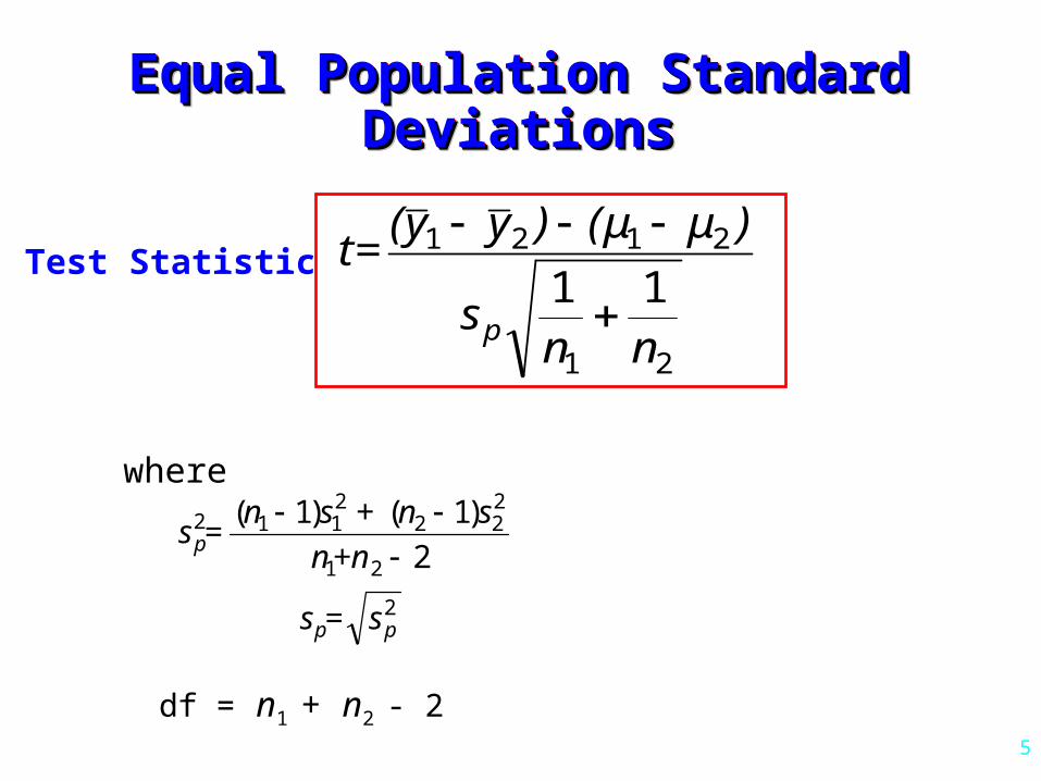
Test Statistic

df = n1 + n2 - 2

nns

)μ(μ)yy( t=

p21

2121

11

s= s

+nn

sn + sn=s

pp

p

2

21

222

2112

2

)1()1(

where

6

Behrens-Fisher ProblemBehrens-Fisher ProblemBehrens-Fisher ProblemBehrens-Fisher Problem

y

2

22

1

21

2121 t~

ns

ns

)(y

1 2 If

7

Satterthwaite’s Approximate t Satterthwaite’s Approximate t StatisticStatistic

Satterthwaite’s Approximate t Satterthwaite’s Approximate t StatisticStatistic

y

1 t

ns

ns

)(y

2

22

1

21

212

1 2 If

2 2 21 2

2 21 2

1 2

( ), ,

1 1

a b s sa b

a b n nn n

df = Approximate t df

(i.e. approximate t)

8

Often-Recommended Strategy Often-Recommended Strategy for Tests on Meansfor Tests on Means

Often-Recommended Strategy Often-Recommended Strategy for Tests on Meansfor Tests on Means

Test Whether 1 = 2 (F-test )– If the test is not rejected, use the 2-sample t statistics,

assuming equal standard deviations– If the test is rejected, use Satterthwaite’s approximate t

statistic

NOTE: This is Not a Wise Strategy– the F-test is highly susceptible to non-normality

Recommended Strategy:– If uncertain about whether the standard deviations are

equal, use Satterthwaite’s approximate t statistic

9

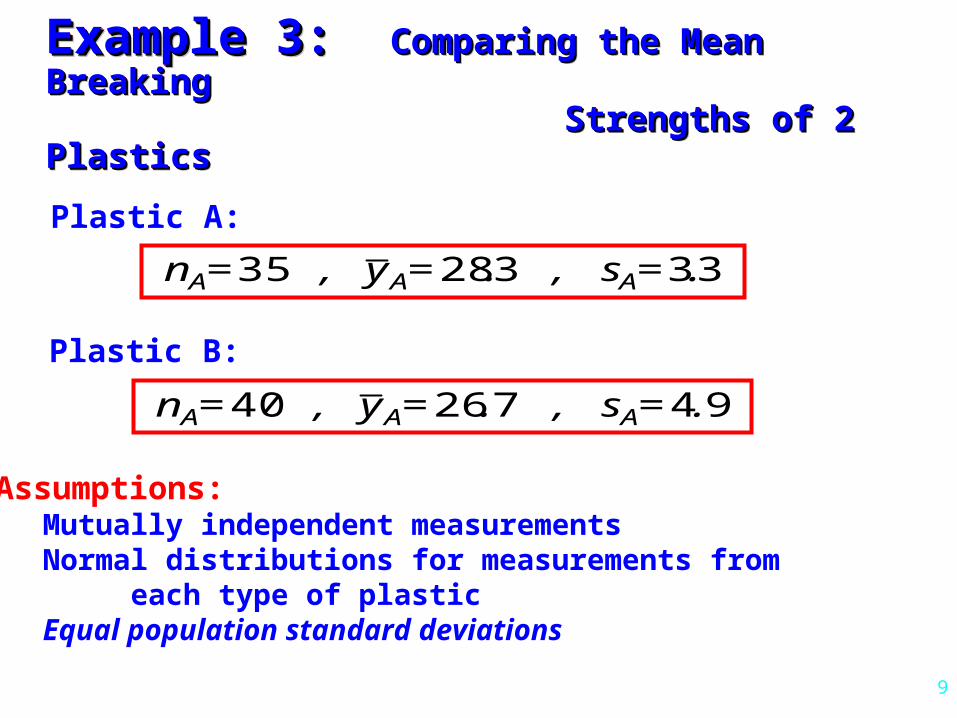
Example 3: Example 3: Comparing the Mean BreakingComparing the Mean Breaking Strengths of 2 Plastics Strengths of 2 PlasticsExample 3: Example 3: Comparing the Mean BreakingComparing the Mean Breaking Strengths of 2 Plastics Strengths of 2 Plastics

Plastic A:

Plastic B:

.= , s.=y , = n AAA 3332835

Assumptions:Mutually independent measurementsNormal distributions for measurements from each type of plasticEqual population standard deviations

.= , s.=y , = n AAA 9472640

10

New diet -- Is it effective?New diet -- Is it effective?

Design:Design:

50 people: randomly assign 25 to go on diet and 25 to eat normally for next month.

Assess results by comparing weights at end of 1 month.

Diet: No Diet:Diet: No Diet:

D

D

X

SND

ND

X

S

Run 2-sample t-test using guidelines we have discussed.

Is this a good design?

11

Better Design:Better Design:

Randomly select subjects and measure them before and after 1-month on the diet.

Subject Before After 1 150 147 2 210 195 : : :

n 187 190

Difference 3 15 :

-3

Procedure: Calculate differences, and analyze differences using a 1-sample test

““Paired t-Test”Paired t-Test”

12

Example 4:Example 4: International Gymnastics International Gymnastics JudgingJudging

Example 4:Example 4: International Gymnastics International Gymnastics JudgingJudging

Contestant 1 2 3 4 5 6 7 8 9 10 11 12Native J udge 6.8 4.5 8.0 7.2 8.7 4.5 6.6 5.8 6.0 8.8 8.7 4.4Foreign J udges 6.7 4.3 8.1 7.2 8.3 4.6 5.4 5.9 6.1 9.1 8.7 4.3

Question: Do judges from a contestant’s country rate their own contestant higher than do foreign judges?

0 : N FH i.e. test

:a N FH

Data:

13

Assignment -- Due Tuesday, Feb. 1

Problems in Ott and Longnecker:# 5.57, page 241 -- parts (a), (b), and (c).

# 6.71, page 330

# 6.83, page 334 (a)

For the hypothesis tests, run the tests using the 4-step procedure I gave in class. Also, in each case, find the p-value.

14

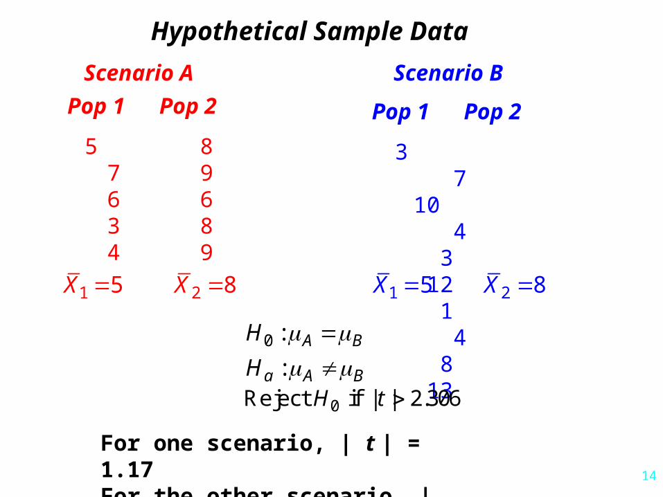
Hypothetical Sample Data

Scenario A

Pop 1 Pop 2

5 8 7 9 6 6 3 8 4 9

Scenario B

Pop 1 Pop 2

3 7 10 4 3 12 1 4 8 131 5X 2 8X 1 5X 2 8X

0 :

:A B

a A B

H

H

0 | | 2.306H t Reject if

For one scenario, | t | = 1.17For the other scenario, | t | = 3.35

15

In general, for 2-sample t-tests:

To show significance, we want the difference between groups 1 2X X( i.e. ) to be large

compared to the variability within groups

1 2

1 1ps

n n(as measured for example by )

16

Begin Thursday, Jan 27 lecture

17

Completely Randomized Design1-Factor Analysis of Variance

(ANOVA)

2 2 21 2 t -

Setting (Assumptions):

- t populations

- populations are normal2

i i

i

- and denote the mean and variance

of the th population

- the sample sizes do not have to all be equal

- mutually independent random samples are taken from the populations

18

1-Factor ANOVA1-Factor ANOVA1-Factor ANOVA1-Factor ANOVA

. . .

19

Question:

1 2 IS ?t

0 1 2: tH

: the means are not all equalaH

Notes:- not directional

i.e. no “1-sided / 2-sided” issues

- alternative doesn’t say that all means are distinct

i.e we test the null hypothesis

20

Completely Randomized Design1-Factor Analysis of Variance

Example data setup where t = 5 and n = 4

21

Notation:

ijy j i- denotes th observation from th population

in i- denotes sample size from th population

.iy i- denotes sample average from th population

..y- denotes sample average of all observations

22

2 2 2.. . .. .

1 1 1 1 1

( ) ( ) ( )t n t t n

ij i ij ii j i i j

y y n y y y y

A Sum-of-Squares Identity

Note: This is for the case in which all sample sizes are equal ( n )

TSS SSB SSW Notation:

In words:

Total SS = SS between samples + within sample SS

Note: Formula for unequal sample sizes given on page 388

23

2 2 2.. . .. .

1 1 1 1 1

( ) ( ) ( )t n t t n

ij i ij ii j i i j

y y n y y y y

TSS SSB SSW Notation:

In words:

TSS(total SS) = total sample variability

SSB(SS between samples) = variability due to factor effects

SSW(within sample SS) = variability due to uncontrolled error

24

Pop 1 5 5 5 5

Pop 2 9 9 9 9

Pop 3 7 7 7 7

2. ..

1

( )t

ii

SSB n y y

What is

2.

1 1

( )t n

ij ii j

SSW y y

What is

25

Pop 1 4 8 3 9

Pop 2 6 10 2 6

Pop 3 5 8 7 4

2. ..

1

( )t

ii

SSB n y y

What is

2.

1 1

( )t n

ij ii j

SSW y y

What is

26

To show significance, we want the difference between groups 1 2y y( i.e. ) to be large

compared to the variability within groups

1 2

1 1ps

n n(as measured for example by )

Recall: For 2-sample t-test to test we use

1 2

1 2

1 1

p

y yt

sn n

0 1 2:H

27

Note: Our test statistic for testing

will be of the form

0 1 2: tH :aH the means are not all equal

/( 1)

/( )

SSB tF

SSW tn t

This has an F distribution

-1 -t tn twith and df when

0H is true

Question: What type of F values lead you to believe the null is NOT TRUE?

28

Analysis of Variance TableAnalysis of Variance TableAnalysis of Variance TableAnalysis of Variance Table

Note:

1 2

T

t

n nt

n n n

if sample sizes are equal

otherwise

2

0 2( 1, )B

TW

sH F F t n t

s We reject at significance level if

29

Note:

2 2W ps s is a generalization of

30

CAR DATA Example

For this analysis, 5 gasoline types (A - E) were to be tested. Twenty carswere selected for testing and were assigned randomly to the groups (i.e. the gasoline types). Thus, in the analysis, each gasoline type was tested on 4 cars. A performance-based octane reading was obtained for each car,and the question is whether the gasolines differ with respect to this octanereading.  

  A

91.7 91.2 90.9 90.6

B

91.7 91.9 90.9 90.9

C

92.4 91.2 91.6 91.0

D

91.8 92.2 92.0 91.4

E

93.1 92.9 92.4 92.4

31

ANOVA Table Output - car data 

 

Source SS df MS F p-value 

Between 6.108 4 1.527 6.80 0.0025  samples

Within 3.370 15 0.225  samples

Totals 9.478 19 

32

F-table -- p.1106

33

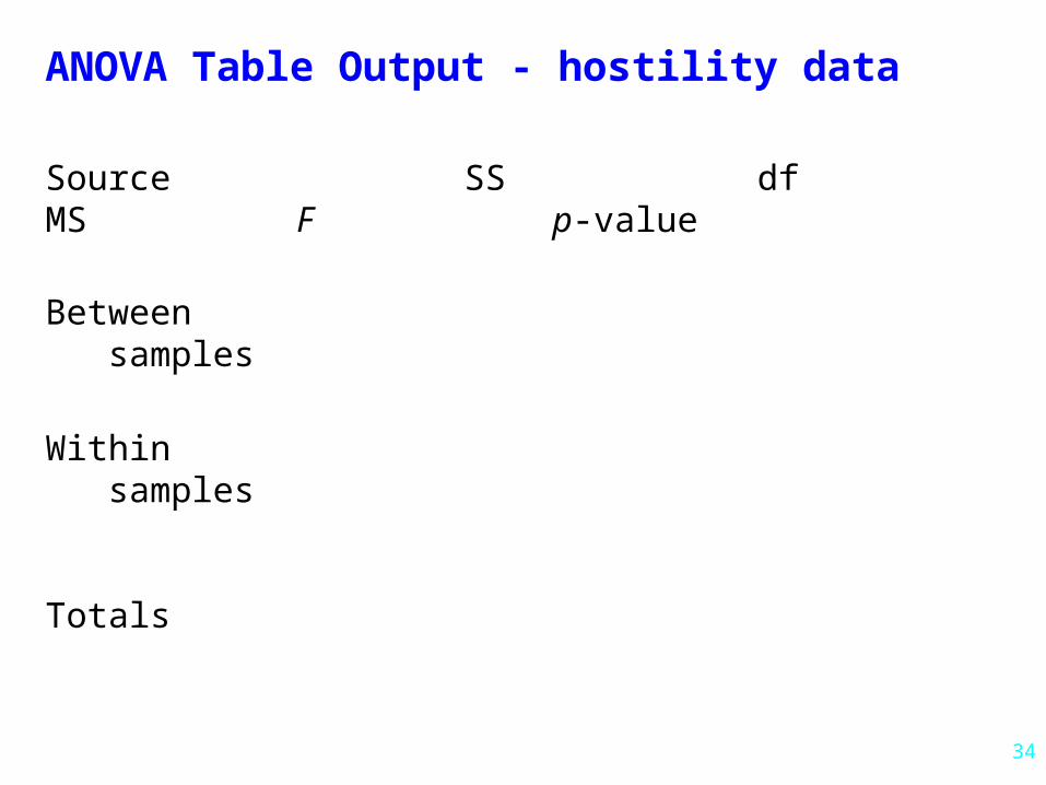
Extracted from From Ex. 8.2, page 390-391

3 Methods for Reducing Hostility

12 students displaying similar hostility were randomly assigned to 3 treatment methods. Scores (HLT) at end of study recorded.

Method 1 96 79 91 85

Method 2 77 76 74 73

Method 3 66 73 69 66

Test: 0 1 2 3:H

34

ANOVA Table Output - hostility data 

 

Source SS df MS F p-value 

Between  samples

Within  samples

Totals