1

ECE 776 Project

Information-theoretic Approaches for Sensor Selection and Placement in Sensor Networks for Target Localization and Tracking

Renita Machado

2

Wireless sensor networks and their applications

Wireless sensor networks (WSNs) are networks of large number of nodes deployed over a region to sense, gather and process data about their environment.

The self organizing capabilities of WSNs enable their use in applications ranging from surveillance, ecology monitoring, bio-monitors and various other applications for developing smart environments.

3

Key challenges in WSNs

Performance measures Coverage Connectivity Optimal redundancy Reliability of network operation

Constraints Power limited nodes Economic constraints for dense deployments

4

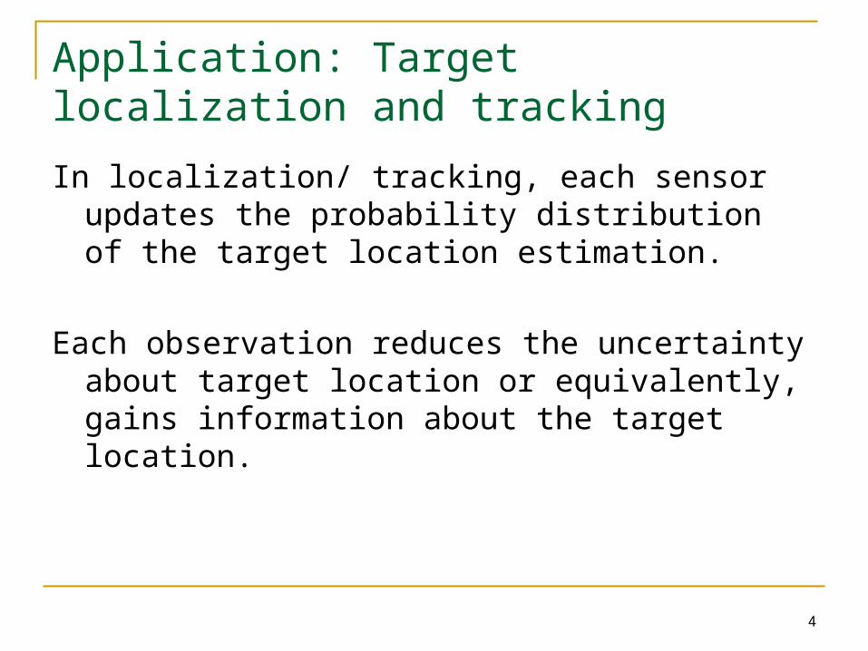
Application: Target localization and tracking

In localization/ tracking, each sensor updates the probability distribution of the target location estimation.

Each observation reduces the uncertainty about target location or equivalently, gains information about the target location.

5

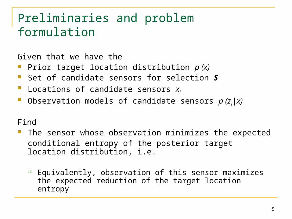
Preliminaries and problem formulation

Given that we have the Prior target location distribution p (x) Set of candidate sensors for selection S Locations of candidate sensors xi

Observation models of candidate sensors p (zi|x)

Find The sensor whose observation minimizes the expected

conditional entropy of the posterior target location distribution, i.e.

Equivalently, observation of this sensor maximizes the expected reduction of the target location entropy

6

Entropy difference in minimizing the uncertainty of localization Reduction of localization uncertainty attributable to a sensor depends

on the difference between

A. Entropy of noise free sensor observation

B. Entropy of that sensor observation model corresponding to the true target location

7

A. Sensor observation model

Sensor observation model corresponding to the true target location Probability distribution of the sensor observation

conditioned on true target location Incorporates observation error from all sources, including

Target Signal modeling error in estimation algorithm used by the sensor Inaccuracy of the sensor hardware

Amount of uncertainty in sensor observation model may depend on the target location.

8

Determination of the sensor observation model Since true target location is unknown during the process of target

localization and tracking, we have to use an estimated target location to approximate the true target location to determine the sensor observation model.

9

Single-modal target location

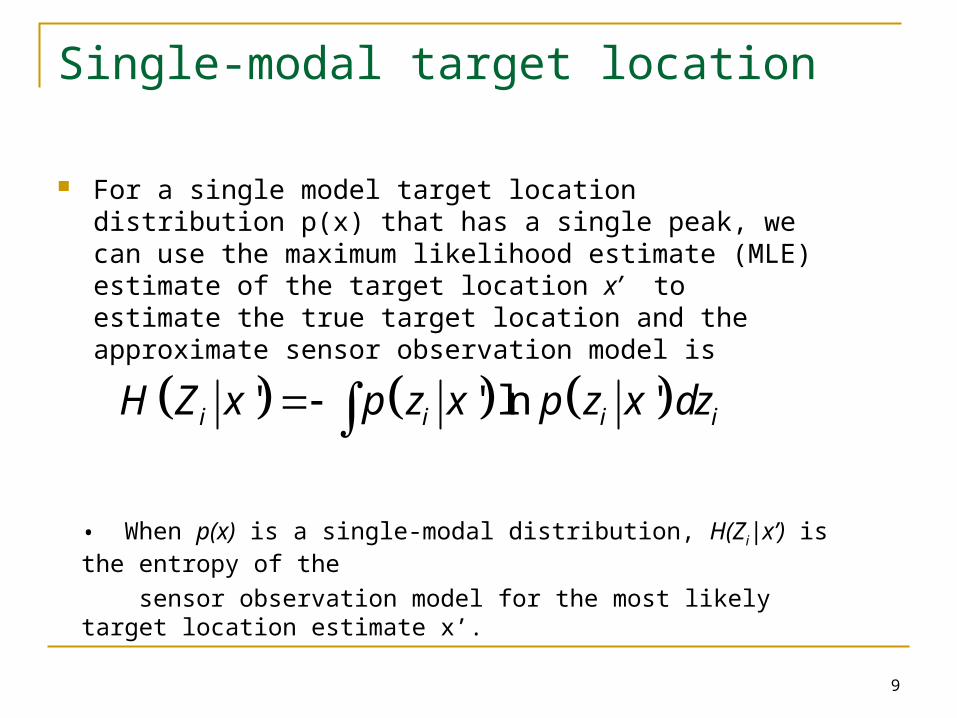
For a single model target location distribution p(x) that has a single peak, we can use the maximum likelihood estimate (MLE) estimate of the target location x’ to estimate the true target location and the approximate sensor observation model is

' ' ln 'i i i iH Z x p z x p z x dz

• When p(x) is a single-modal distribution, H(Zi|x’) is the entropy of the

sensor observation model for the most likely target location estimate x’.

10

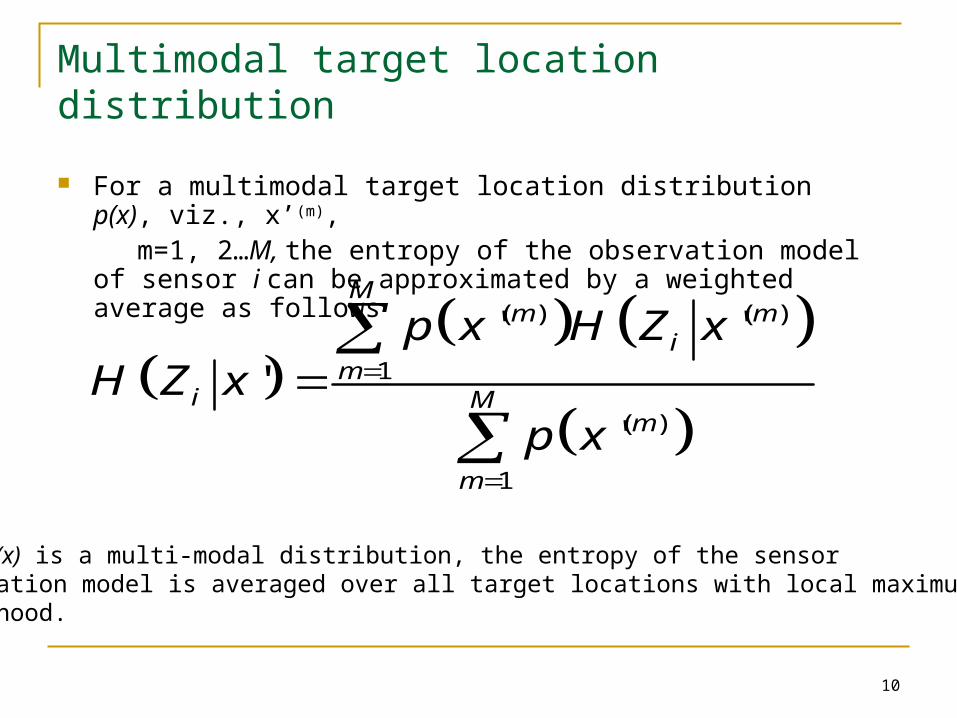
Multimodal target location distribution

For a multimodal target location distribution p(x), viz., x’(m), m=1, 2…M, the entropy of the observation model of sensor i can be

approximated by a weighted average as follows

( ) ( )

1

( )

1

' ''

'

Mm m

im

i Mm

m

p x H Z xH Z x

p x

When p(x) is a multi-modal distribution, the entropy of the sensor observation model is averaged over all target locations with local maximum likelihood.

11

Relationship of H (Zi|x) to H(Zi|x’)

H (Zi|x) is actually the entropy of the sensor observation model averaged over all possible target locations.

When the entropy of the sensor observation model H(Zi|x) changes slowly with respect to the target location x, H(Zi|x’) reasonably approximates H (Zi|x).

12

B. Noise free sensor observation

Noise free sensor observation No error is introduced in the sensor observation

Let Ziv = noise-free observation of sensor i.

Ziv assumes no randomness in the process of observation regarding the

target location. Hence it is a function of target location X and sensor location xi.

The target location X is a random variable, sensor location xi is a deterministic quantity.

Hence the noise free sensor observation is a random variable.

13

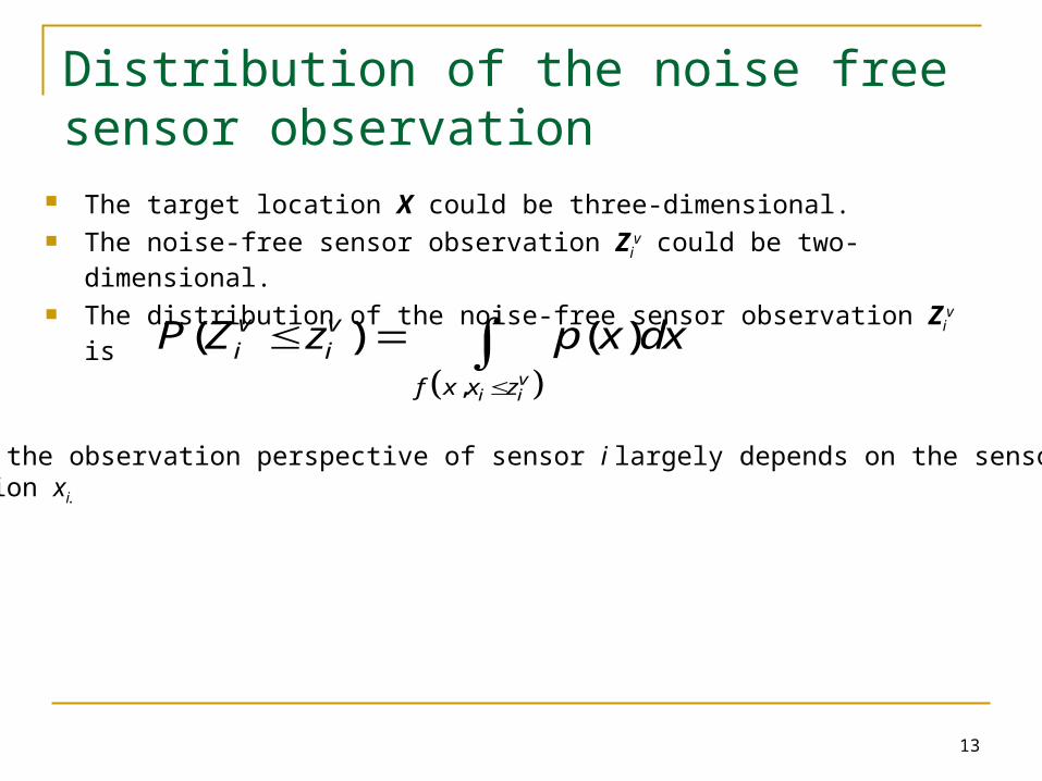
Distribution of the noise free sensor observation

The target location X could be three-dimensional. The noise-free sensor observation Zi

v could be two-dimensional.

The distribution of the noise-free sensor observation Ziv is

,

( ) ( )v

i i

v vi i

f x x z

P Z z p x dx

where the observation perspective of sensor i largely depends on the sensorlocation xi.

14

Computing the noise free sensor observation distribution and its entropy Let X be the set of target location grid values with non-trivial probability

density, Let Z be the set of noise-free sensor observation grid values of non-trivial

probability density For each grid point zi

v є Z, initialize p(ziv) to zero;

For each grid point x є X, the corresponding grid point ziv є Z is calculated

using

Ziv = f (X, xi)

The probability is updated as p (zi

v)= p (ziv) + p (x)

Normalize p (ziv) to make the total probability of Z to be 1.

From p (ziv), we calculate the noise-free sensor observation entropy H(Zi

v).

15

Relationship of H(Ziv) to H(Zi)

H(Zi) is the entropy of the predicted sensor observation distribution,

( )i ip z p z x p x

The predicted sensor observation distribution p(Zi) becomes the noise-freesensor observation p(zi

v) when the sensor observation model p(zi|x) is deterministic without any uncertainty.

The uncertainty in the sensor observation model p(zi|x) makes the predicted sensor observation entropy H(Zi) larger than the noise-free sensor observation entropy H(Zi

v) .

16

Since ( )vi iH Z H Z and ( ') ( )i iH Z x H Z x

( ; ) ( ) ( | )

( ) ( ')

i i i

vi i

I X Z H Z H Z X

H Z H Z x

Thus, the sensor with the maximum entropy difference

( ; ) ( ) ( ')vi i iI X Z H Z H Z x

probably also has the maximum mutual information.

When the sensor observation model has only a small amount of uncertainty,

( )vi iH Z H Z

Approximations to the mutual-information calculation

17

Why not select the mutual information I(X;Zi)? For target location X and the predicted sensor observation Zi

( , )( ; ) ( , ) ln

( ) ( )i

i i ii

p x zI X Z p x z dxdz

p x p z

The target location could be 3-dimensional and the sensor observation could be 2-dimensional.

Then I(X;Zi) could be a complex integral in the joint state space of 5 dimensions.

Thus, the total cost to select one of K candidate sensors is O(n5).

18

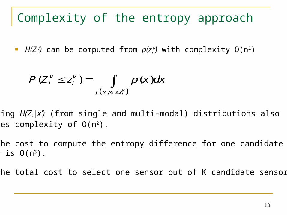
Complexity of the entropy approach

H(Ziv) can be computed from p(zi

v) with complexity O(n2)

,

( ) ( )v

i i

v vi i

f x x z

P Z z p x dx

Computing H(Zi|x’) (from single and multi-modal) distributions also requires complexity of O(n2).

Thus the cost to compute the entropy difference for one candidate sensor is O(n3).

Thus the total cost to select one sensor out of K candidate sensors isO(n3).

19

Reduction in complexity

The computational complexity of the mutual information approach is greater than that of the entropy difference approach.

With power constraints and processing complexity constraints, the entropy difference approach fares better than the mutual information approach for selecting a sensor for target localization.

20

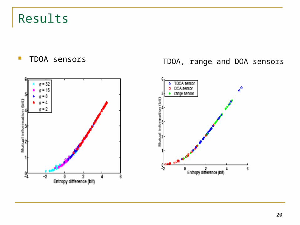
Results

TDOA sensors TDOA, range and DOA sensors

21

Conclusions

The entropy difference approach is simpler to calculate than the mutual information criterion for sensor selection.

A sub-optimal sensor can be selected without retrieving sensor data.

Reference H.Wang, K.Yao and D.Estrin, “Information-theoretic approaches for sensor selection

and placement in sensor networks for target localization and tracking”, CENS Technical Report #52, 2005.