materials

Article

Response Surface Method Analysis of Chemically StabilizedFiber-Reinforced Soil

Abdullah Almajed 1,* , Dinesh Srirama 2 and Arif Ali Baig Moghal 2

�����������������

Citation: Almajed, A.; Srirama, D.;

Moghal, A.A.B. Response Surface

Method Analysis of Chemically

Stabilized Fiber-Reinforced Soil.

Materials 2021, 14, 1535. https://

doi.org/10.3390/ma14061535

Academic Editors: Bahman Ghiassi

and Angelo Marcello Tarantino

Received: 29 December 2020

Accepted: 18 March 2021

Published: 21 March 2021

Publisher’s Note: MDPI stays neutral

with regard to jurisdictional claims in

published maps and institutional affil-

iations.

Copyright: © 2021 by the authors.

Licensee MDPI, Basel, Switzerland.

This article is an open access article

distributed under the terms and

conditions of the Creative Commons

Attribution (CC BY) license (https://

creativecommons.org/licenses/by/

4.0/).

1 Department of Civil Engineering, College of Civil Engineering, King Saud University,Riyadh 11421, Saudi Arabia

2 Department of Civil Engineering, National Institute of Technology, Warangal 506004, Telangana State, India;dinesh1991@student.nitw.ac.in (D.S.); baig@nitw.ac.in or reach2arif@gmail.com (A.A.B.M.)

* Correspondence: alabduallah@ksu.edu.sa

Abstract: One of the significant issues persisting in the study of soil stabilization is the establishmentof the optimum proportions of the quantity of stabilizer to be added to the soil. Determining optimumsolutions or the most feasible remedies for the utilization of stabilizing products in terms of theirdose rates has become a significant concern in major civil engineering design projects. Using theresponse surface methodology, this study primarily focused on investigating the optimal levels ofreinforcement fiber length (FL), fiber dosage (FD), and curing time (CT) for geotechnical parametersof stabilized soil. To realize this objective, an experimental study was undertaken on the Californiabearing ratio (CBR) and unconfined compressive strength (UCS). Hydraulic conductivity (HC) testswere also performed, with stabilizer proportions of 6–12 mm for the FL and 0.2–0.6% for the FDcalculated for the total dry weight of soil and 6% lime (total weight of dry soil). The curing timesused for testing were 0, 7, and 14 days for the CBR tests; 60, 210, and 360 days for the UCS tests; and7, 17, and 28 days for the HC tests. All practical experiments were conducted with experimentaltechniques using stabilizer proportions and curing times. The FL, FD, CT, CBR, UCS, and HCresponse factors were determined using the central composite design. The results point toward astatistically significant model constructed (p ≤ 0.05) using the analysis of variance. The results fromthis optimization procedure show that the optimal values for the FL, FD, and CT were 11.1 mm, 0.5%,and 13.2 days, respectively, as these provided the maximum values for the CBR; 11.7 mm for the FL,0.3% for the FD, and 160 days for the CT corresponded to the maximum values for the UCS; and10.5 mm for the FL, 0.5% for the FD, and 15 days for the CT led to the minimum value for the HC. Inpractice, the suggested values may be useful for experiments, especially for preliminary assessmentsprior to stabilization.

Keywords: response surface methodology; optimization; lime; fiber; stabilization

1. Introduction

Site feasibility is the major hindrance in most civil engineering projects. In the majorityof civil engineering projects worldwide, expansive soils have substantial geotechnical andstructural design-related issues, with economic difficulties estimated to entail costs ofseveral billion dollars annually [1–3]. These soils are usually rich in montmorillonite min-eral, which causes significant volume changes (shrink/swell) with variations in moisturecontent [4,5].

In many instances, naturally available soils require lasting alternatives because theydo not meet specific geotechnical properties [6]. Improvement in the various geotechnicalproperties of soil can be achieved by stabilization with suitable materials. Recent advanceshave shown a rising interest in chemical and bio-geochemical alterations of soils hatenhance their geotechnical properties [5,7]. Among these methods, lime stabilization is themost sought after technique due to its versatility and innate potential in addressing thedistress-related issues of expansive plastic fines [8–11]. Even though lime usage affects the

Materials 2021, 14, 1535. https://doi.org/10.3390/ma14061535 https://www.mdpi.com/journal/materials

Materials 2021, 14, 1535 2 of 18

rapid and significant loss in strength resulting from brittle failure characteristics, manyresearchers have found it most effective in enhancing expansive soil properties. Thepast few years have seen growing attention paid to expansive soil reinforcement withdifferent fibers. The reinforcements of various shapes and dimensions are made out ofgeo-synthetic materials or short fiber strips [12]. A notable increase in the soil index andengineering properties of cohesive soil was achieved after strengthening with discretepolypropylene fiber [13]. Many researchers have studied the effects of polypropylene fibercontent, polypropylene fiber length (FL), lime content, and curing time (CT) on the variousengineering properties of expansive soil [9,14,15]. When amended with the soil medium,polypropylene fiber materials demonstrate proven functionality in durability and sustainsoil index and engineering properties improvements in the long run [14,15].

Fiber Cast (FC) fibers have a better swell-limiting efficiency in the absence of limetreatment [16]. The nature and type of fiber, dosage and length have a considerable impacton the California bearing ratio (CBR) values of natural soils and soils stabilized usinglime [17]. Mean FC and Fiber Mesh (FM) dimensions and concentrations are vital in design-ing the variables of fiber-reinforced lime-amended expansive soils, predominantly affectingthe subgrade stability [18]. One of the significant issues persisting in soil stabilizationis the establishment of an optimum quantity of stabilizer to be added to the soil. Thisinvolves an excessive amount of energy and time for investigation and necessitates anenormous number of experiments. These downsides could be well avoided by determin-ing the optimal or best possible solutions using approximation concepts, mathematicalsystem modeling, or optimization procedures [6–15]. The inspiration behind the usage ofoptimization procedures lies in quality improvement and in cost reduction.

Experimentation based on the measurement of one or more responses (variables)plays a significant part in several science and technology areas. Planning and designingexperiments, analyzing the results and observing the process and the system operation arenecessary to obtain a final result. The response surface methodology (RSM) is one of themost commonly used experimental designs for optimization [19]. It is a compilation of bothnumerical and statistical methods helpful for building an empirical model and optimizationprocess parameters and is mostly used in finding the interaction of numerous affectingfactors [20]. Through the design of experiments, the RSM expels systematic errors andreduces the number of experiments required to obtain the optimum values. It comprises aset of mathematical and analytical methods that are valuable for establishing the buildingof the empirical design and enhancing and maximizing process specification. The RSM canalso be utilized to discover the interaction of numerous impacting aspects [21]. The RSMoptimization involves three primary steps: (1) statistically calculated trials; (2) estimatingthe coefficients; and (3) predicting the response and validating the model adequacy withthe experimental arrangement [22].

The present study examined the determination of input variables (i.e., amount andlength of fibers and CT) that could potentially offer the optimum values of various geotech-nical parameters, such as the unconfined compression strength (UCS), hydraulic con-ductivity (HC), and California bearing ratio, through optimization using face-centeredcentral composite design (FCCCD) in conjunction with an RSM study of regular expansivesemi-arid soil from the municipality of Al-Ghat. The addition of lime (quick lime) wasconsidered to ensure the proper bonding between clay particles and fiber components,with 6% lime dosage [23]. The impacts of various values for the soil fiber dosage (FD)(0.2%, 0.4%, and 0.6% by dry weight), the FL (6, 9, and 12 mm), and the CT (0–14 days forthe CBR, 60–360 for the UCS, and 7–28 days for the HC) on the geotechnical parametersstudied for the targeted soil using the RSM were evaluated. The optimum values for soilstabilization for various applications are presented.

Materials 2021, 14, 1535 3 of 18

2. Experimental Investigation2.1. Materials

The soil used in this study was obtained from the municipality of Al-Ghat where thesoil is known to have distinct mineralogical and plasticity properties. The soil is classifiedas clay of high plasticity (CH) according to the Unified Soil Classification System (USCS).The maximum dry density and optimum moisture content were 1.64 kN/m3 and 23%,respectively. Its plasticity index is 31%. In its natural state, the soil has 3.2% moisturecontent and had a specific gravity value of 2.85. Analytical grade quick lime (supplied byWinlab Chemicals, UK) was utilized as a chemical additive. Polypropylene fibers (FiberCast) acquired from Propex Operating Company (LLC, UK) were used. This fiber hasvery low electrical conductivity and high acid and salt resistance. The tensile strengthwas found to be 440 N/mm2. The melting and ignition points were found to be 324 ◦F(162 ◦C) and 1100 ◦F (593 ◦C), respectively. The fiber is alkali-proof and has zero waterabsorption ability.

2.2. Software Used

Design-Expert, released by Stat-Ease Inc., is an open-source statistical software pack-age for building full quadratic models using RSM and performing analysis of variance(ANOVA). It provides powerful tools for designing an ideal experiment in terms of process,mixture, or a combination of factors and components.

2.3. Sample Preparation and Experimental Procedure

Lime addition (6% by dry weight of soil) to dry soil was carried out prior to mixingfibers. Close attention was paid to the mixing process to maintain a homogenous mix-ture [24]. All samples were compacted at their maximum dry density values in accordancewith ASTM D698 [25]. Following the proper mixing of the respective fibers for each mix(based on the dry weight of soil), tests were performed following the relevant codes men-tioned in Table 1. For hydraulic conductivity tests, the compacted specimen along witha Perspex hydraulic conductivity mold were kept in a desiccator, maintaining a relativehumidity of more than 95%, and cured for 7 and 28 days. For the unconfined compressiontests, the compacted soil samples wrapped in plastic were preserved in humidity-controlledchambers (maintained at 100% relative humidity) to avoid any moisture movements. Thesamples were cured for 60 and 360 days, following which the specimen weight was noted.Any sample which recorded a loss of weight of 5% due to heat or hydration was rejectedprior to testing. For CBR tests, the force required for a penetration of up to 12.5 mm wasdetermined on the samples cured for 14 days (and also for the immediate case at 0 days ofthe curing period), which were tested at their respective optimum moisture content andmaximum dry density values. For each geotechnical parameter, samples were tested intriplicate. The dispersion of the results was found to be within 5% confidence limits, as perrelevant ASTM standards, for each test considered. The experimental CBR values underthe soaked condition, the UCS values, the and HC values were determined for respectivecuring times of 0–14 days for the CBR, 60–360 days for the UCS, and 7–28 days for the HC(Tables 2–4, respectively).

Table 1. Testing procedures adopted.

Property Value for Untreated Soil (Without Limeand Fiber) Relevant Code

Liquid limit, plastic limit and plasticity Index 66%, 32%, and 34% ASTM D4318 [26]Specific gravity 2.85 ASTM D854 [27]

Bar linear shrinkage test 31% Tex-107-E [28]Unconfined compression strength test 598.11 kPa ASTM D2166 [29]One-dimensional fixed ring oedometer

Consolidation test0.109 (compression index) and 0.069

(swell index) ASTM D2435 [30]

Hydraulic conductivity 6.77 × 10−7 (cm/s) ASTM D5084 [31]California bearing ratio test 5.96 ASTM D1883 [32]

Materials 2021, 14, 1535 4 of 18

Table 2. Experimental California bearing ratio (CBR) values under the soaked condition.

Fiber Length (mm) Fiber Dosage (%) Curing Time (days) CBR (%)

6 0.2 0 116 0.4 0 11.76 0.6 0 12.56 0.2 7 16.36 0.4 7 17.76 0.6 7 19.16 0.2 14 24.66 0.4 14 27.16 0.6 14 29.79 0.2 0 11.49 0.4 0 12.19 0.6 0 12.99 0.2 7 17.29 0.4 7 18.59 0.6 7 19.99 0.2 14 26.29 0.4 14 28.59 0.6 14 30.812 0.2 0 11.812 0.4 0 12.612 0.6 0 13.312 0.2 7 18.112 0.4 7 19.312 0.6 7 20.612 0.2 14 27.912 0.4 14 29.912 0.6 14 31.8

Table 3. Experimental values of the unconfined compression strength (UCS).

Fiber Length (MM) Fiber Dosage (%) Curing Time (days) UCS (kPa)

6 0.2 60 17676 0.4 60 20706 0.6 60 23906 0.2 210 19966 0.4 210 19986 0.6 210 21106 0.2 360 25056 0.4 360 19126 0.6 360 262012 0.2 60 257912 0.4 60 241212 0.6 60 228712 0.2 210 317112 0.4 210 291212 0.6 210 267312 0.2 360 288112 0.4 360 258912 0.6 360 2412

Materials 2021, 14, 1535 5 of 18

Table 4. Experimental values of the hydraulic conductivity (HC).

Fiber Length (mm) Fiber Dosage (%) Curing Time (days) HydraulicConductivity (cm/s)

6 0.2 7 6.21 × 10−7

6 0.4 7 8.23 × 10−7

6 0.6 7 3.14 × 10−6

6 0.2 17 2.55 × 10−8

6 0.4 17 6.72 × 10−8

6 0.6 17 8.27 × 10−7

6 0.2 28 1.69 × 10−8

6 0.4 28 5.63 × 10−8

6 0.6 28 4.77 × 10−7

12 0.2 7 4.15 × 10−6

12 0.4 7 3.71 × 10−6

12 0.6 7 1.85 × 10−5

12 0.2 17 3.66 × 10−7

12 0.4 17 5.28 × 10−7

12 0.6 17 8.37 × 10−6

12 0.2 28 2.63 × 10−7

12 0.4 28 4.22 × 10−7

12 0.6 28 3.86 × 10−6

2.4. Experimental Results

Table 2 reveals that CBR characteristics were significantly increased with curingperiod. The presence of lime triggered the formation of cementitious compounds, resultingin higher CBR values. Along similar lines, the UCS values increased significantly up to210 days, after which there was not much of a significant increase in the values. Beyond210 days of the curing period, the readily available reactive silica was consumed, resultingin a net reduction in the pH of the soil-system, and thus there was no further contributionto any increase in strength. Hence, the rate of gain in the UCS from 210 to 360 daysproceeded at a slower pace, as seen from Table 3. On the other hand, the HC values offiber-treated lime-amended specimens increased with the addition of fiber compared to theuntreated case, as seen from Table 4. With an increase in curing period, the HC values werereduced significantly, which can be attributed to the formation of cementitious compoundsdue to the addition of lime, making the treated soil less conductive. Similar observationshave been reported by Moghal et al. [14–18] for fiber-reinforced lime-blended expansivesemi-arid soils.

3. RSM3.1. Experimental Design

For the experimental design, a face-centered central composite design (FCCCD) wasemployed to build the RSM model. A three-factor experimental design, consisting ofeight factor points representing the upper and lower limits of the three input variables,six axial points representing how far outside the factorial limits a parametric value can becomprehensive, and six center points representing the mean values of the input variables,was created.

3.2. Model Development

The inclusion rates of the independent variables were the fiber lengths of 6, 9, and12 mm, fiber dosages of 0.2, 0.4, and 0.6% by soil dry weight, and CTs of 0–14 days. TheFCCCD was employed, which used only three levels, “1,” “0”, and “−1”, representing themaximum, mean, and minimum actual values of the input variables, respectively. Table 5lists the experimental levels of each variable. A quadratic model with three factors and threelevels with 95% confidence levels was employed to evaluate the RSM model. The backwardelimination technique was applied with only statistically significant terms to represent

Materials 2021, 14, 1535 6 of 18

the relationship between the input factors and the output response variables (p ≤ 0.05).Tables 6–8 present the values obtained from the experimental procedure and measured andpredicted values from the RSM models of the CBR, UCS, and HC, respectively.

Table 5. Experimental levels of each variable.

VariablesLevel

−1 0 1

Fiber length 6 mm 9 mm 12 mmFiber dosage 0.2% 0.4% 0.6%

CBR curing time 0 days 7 days 14 daysUCS curing time 60 days 210 days 360 daysHC curing time 7 days 17 days 28 days

Table 6. Face-centered central composite design (FCCCD) experiment values and CBR results.

Design Program CBR (%)

FL FD CT FL(mm) FD (%) CT (Days) Actual RSM

−1 −1 −1 6 0.2 0 11 10.88−1 1 −1 6 0.6 0 12.5 12.63−1 −1 1 6 0.2 14 24.6 24.78−1 1 1 6 0.6 14 29.7 29.54−1 0 0 6 0.4 7 17.7 17.630 −1 0 9 0.2 7 17.2 17.070 1 0 9 0.6 7 19.9 20.0240 0 −1 9 0.4 0 12.1 12.110 0 1 9 0.4 14 28.5 28.471 −1 −1 12 0.2 0 11.8 11.951 1 −1 12 0.6 0 13.3 13.111 −1 1 12 0.2 14 27.9 27.761 1 1 12 0.6 14 31.8 31.911 0 0 12 0.4 7 19.3 19.36

Table 7. FCCCD experiment values and UCS results.

Design Program UCS (kPa)

FL FD CT FL(mm) FD (%) CT (Days) Actual RSM

−1 −1 1 6 0.2 60 1766.17 1781.52−1 1 1 6 0.6 60 2390.65 2285.8−1 −1 −1 6 0.2 360 2505.39 2414.71−1 1 −1 6 0.6 360 2620.12 2581.46−1 0 0 6 0.4 210 1998.26 2290.240 −1 0 9 0.2 210 2582.61 2503.180 1 0 9 0.6 210 2391.21 2493.610 0 1 9 0.4 60 2223.01 2125.130 0 0 9 0.4 210 2453.82 2407.941 −1 1 12 0.2 60 2579.15 2641.421 1 1 12 0.6 60 2287.39 2388.041 −1 −1 12 0.2 360 2880.73 2953.501 1 −1 12 0.6 360 2411.96 2362.591 0 0 12 0.4 210 2911.87 2642.87

Materials 2021, 14, 1535 7 of 18

Table 8. FCCCD experiment values and HC results.

Design Program HC (cm/s)

FL FD CT FL(mm) FD (%) CT (Days) Actual RSM

−1 −1 1 6 0.2 7 6.21 × 10−7 1.47 × 10−7

1 −1 1 12 0.2 7 4.15 × 10−6 4.64 × 10−6

−1 1 1 6 0.6 7 3.14 × 10−6 4.7 × 10−6

1 1 1 12 0.6 7 1.85 × 10−5 1.65 × 10−5

−1 −1 −1 6 0.2 28 1.69 × 10−8 1.92 × 10−6

1 −1 −1 12 0.2 28 2.63 × 10−8 −7.8 × 10−7

−1 1 −1 6 0.6 28 4.77 × 10−7 4.81 × 10−7

1 1 −1 12 0.6 28 3.86 × 10−6 5.06 × 10−6

−1 0 0 6 0.4 17 6.72 × 10−8 −2.4 × 10−6

1 0 0 12 0.4 17 5.28 × 10−7 3.37 × 10−6

0 −1 0 9 0.2 17 1.95 × 10−7 −4.9 × 10−7

0 1 0 9 0.6 17 4.59 × 10−6 5.7 × 10−6

0 0 1 9 0.4 7 2.26 × 10−6 3.87 × 10−6

0 0 −1 9 0.4 28 2.39 × 10−7 −9.5 × 10−7

0 0 0 9 0.4 17 2.97 × 10−7 2.43 × 10−7

3.3. Validation of the Built Model

In the response surface method, the relationships between the independent anddependent variables were determined using multiple regression techniques. The regressionequations used to build models to determine the relationships between variables andrepresent the total effect of all variables obtained from the experimental or actual valueshad to be validated with the approximation values obtained from the models. It was alsoessential to verify whether any of the least-squares regression assumptions have beenviolated. The coefficient (R2), adjusted R2 (Adj R2), predicted R2 (Pred R2), and adequateprecision (AP) values were then computed.

4. Results and Discussions4.1. Statistical Assessment of the Experimental Results of the CBR

The influence on the ANOVA dependent variable resulting from different independentfactors was evaluated using a parametric statistical technique. The influence of independentfactors (i.e., FL, FD, and CT) and their interactions on the response variable (i.e., theCBR value) was studied with ANOVA, which is a useful statistical tool for describingthe interactions of variables with each other. As previously mentioned, the statisticalsignificance of independent parameters (i.e., FL, FD, and CT) with regard to the dependentvariable (i.e., the CBR value) experimental results at a 95% confidence level was analyzedusing a full quadratic model. The statistically insignificant terms, with p greater than 0.05,were removed by performing a backward analysis on the full quadratic equation. Thepercentage contributions to the response parameters in the model built were determined.ANOVA was performed, with the results containing enumerated terms (Table S1).

Table 6 compiles the CBR values obtained through the experiments performed inthe lab and measured from the FCCCD experiments designed using Design-Expert soft-ware. The following models (Equation (1)) were developed for the CBR values using theregression coefficients summarized in Table S4.

CRB = (8.65646 + (0.251732 × FD) + (5.10504 × FL) + (0.239471 × CT) − (0.250000 × (FD × FL))+ (0.022619 × (FD × CT)) + (0.535714 × (FL × CT)) + (0.036507 × CT2)

(1)

Table S1 shows p < 0.05, which indicates significant model terms.The model F value of 33,444.15 indicates the model significance. This calculation

determines the ratio of explained to unexplained variance. Computations were performedfor the statistically significant parameters, whereas insignificant parameters (with p > 0.05)were removed using backward analysis from a complete RSM quadratic model. Figure 1

Materials 2021, 14, 1535 8 of 18

depicts the plot of predicted versus actual values for the CBR and Figure 2 depicts thecontributions of each parameter to the constructed RSM model.

Materials 2021, 14, 1535 8 of 19

Table 6 compiles the CBR values obtained through the experiments performed in the lab and measured from the FCCCD experiments designed using Design-Expert software. The following models (Equation (1)) were developed for the CBR values using the regres-sion coefficients summarized in Table S4. 𝐶𝐵𝑅 = 8.65646 + (0.251732 × 𝐹𝐷) + (5.10504 × 𝐹𝐿) + (0.239471 × 𝐶𝑇) − 0.250000 × (𝐹𝐷 × 𝐹𝐿)+ 0.022619 × (𝐹𝐷 × 𝐶𝑇) + 0.535714 × (𝐹𝐿 × 𝐶𝑇) + (0.036507 × 𝐶𝑇 ) (1)

Table S1 shows p < 0.05, which indicates significant model terms. The model F value of 33,444.15 indicates the model significance. This calculation de-

termines the ratio of explained to unexplained variance. Computations were performed for the statistically significant parameters, whereas insignificant parameters (with p > 0.05) were removed using backward analysis from a complete RSM quadratic model. Figure 1 depicts the plot of predicted versus actual values for the CBR and Figure 2 depicts the contributions of each parameter to the constructed RSM model.

The CBR values built using the RSM model and Equation (1) were validated for the R2, Adj R2, Pred R2, and AP statistics (Table 7). With a difference of less than 0.2, the Pred R2 of 0.9996 was in reasonable agreement with the Adj R2 of 0.9997. As shown in Table S1, the R2 of the model was 0.9996 (close to 1), indicating the variation of the response variable through input factors by robust fitting.

Adequate precision is desirable, with a ratio greater than 4. A 510.030 ratio indicates an adequate signal to ensure the possibility of using the model in navigating the design space. The Pred R2, explaining the variance in the new data of the constructed model, was 0.9996 (Table S1), indicating that approximately 99.96% of the variability in the estimation of the new response values can be explained by the built RSM model.

Figure 1. Plot of predicted vs. actual values for the CBR

Figure 1 shows that the prediction provided by the model equation vs. the experi-mental values was a statistically good match. Figure 2 displays the average probability of residuals for a response, confirming whether a normal distribution follows the standard deviations between the actual and predicted response values [33,34].

Actual

Pred

icted

10

15

20

25

30

35

10 15 20 25 30 35

Figure 1. Plot of predicted vs. actual values for the CBR

Materials 2021, 14, 1535 9 of 19

Figure 2. Plot of normal probability of residuals

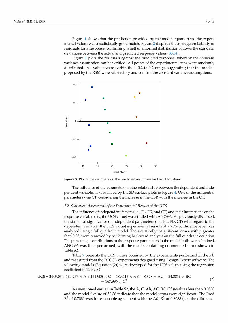
Figure 3 plots the residuals against the predicted response, whereby the constant var-iance assumption can be verified. All points of the experimental runs were randomly dis-tributed. All values were within the −0.2 to 0.2 range, suggesting that the models proposed by the RSM were satisfactory and confirm the constant variance assumptions.

Figure 3. Plot of the residuals vs. the predicted responses for the CBR values

The influence of the parameters on the relationship between the dependent and in-dependent variables is visualized by the 3D surface plots in Figure 4. One of the influential parameters was CT, considering the increase in the CBR with the increase in the CT.

Residuals

Norm

al %

Prob

abilit

y

-0.2 -0.1 0 0.1 0.2

1

510

2030

50

7080

9095

99

Predicted

Resid

uals

-0.2

-0.1

0

0.1

0.2

10 15 20 25 30 35

0

Figure 2. Plot of normal probability of residuals

The CBR values built using the RSM model and Equation (1) were validated for theR2, Adj R2, Pred R2, and AP statistics (Table 7). With a difference of less than 0.2, the PredR2 of 0.9996 was in reasonable agreement with the Adj R2 of 0.9997. As shown in Table S1,the R2 of the model was 0.9996 (close to 1), indicating the variation of the response variablethrough input factors by robust fitting.

Adequate precision is desirable, with a ratio greater than 4. A 510.030 ratio indicatesan adequate signal to ensure the possibility of using the model in navigating the designspace. The Pred R2, explaining the variance in the new data of the constructed model, was0.9996 (Table S1), indicating that approximately 99.96% of the variability in the estimationof the new response values can be explained by the built RSM model.

Materials 2021, 14, 1535 9 of 18

Figure 1 shows that the prediction provided by the model equation vs. the experi-mental values was a statistically good match. Figure 2 displays the average probability ofresiduals for a response, confirming whether a normal distribution follows the standarddeviations between the actual and predicted response values [33,34].

Figure 3 plots the residuals against the predicted response, whereby the constantvariance assumption can be verified. All points of the experimental runs were randomlydistributed. All values were within the −0.2 to 0.2 range, suggesting that the modelsproposed by the RSM were satisfactory and confirm the constant variance assumptions.

Materials 2021, 14, 1535 9 of 19

Figure 2. Plot of normal probability of residuals

Figure 3 plots the residuals against the predicted response, whereby the constant var-iance assumption can be verified. All points of the experimental runs were randomly dis-tributed. All values were within the −0.2 to 0.2 range, suggesting that the models proposed by the RSM were satisfactory and confirm the constant variance assumptions.

Figure 3. Plot of the residuals vs. the predicted responses for the CBR values

The influence of the parameters on the relationship between the dependent and in-dependent variables is visualized by the 3D surface plots in Figure 4. One of the influential parameters was CT, considering the increase in the CBR with the increase in the CT.

Residuals

Norm

al %

Prob

abilit

y

-0.2 -0.1 0 0.1 0.2

1

510

2030

50

7080

9095

99

Predicted

Resid

uals

-0.2

-0.1

0

0.1

0.2

10 15 20 25 30 35

0

Figure 3. Plot of the residuals vs. the predicted responses for the CBR values

The influence of the parameters on the relationship between the dependent and inde-pendent variables is visualized by the 3D surface plots in Figure 4. One of the influentialparameters was CT, considering the increase in the CBR with the increase in the CT.

4.2. Statistical Assessment of the Experimental Results of the UCS

The influence of independent factors (i.e., FL, FD, and CT) and their interactions on theresponse variable (i.e., the UCS value) was studied with ANOVA. As previously discussed,the statistical significance of independent parameters (i.e., FL, FD, CT) with regard to thedependent variable (the UCS value) experimental results at a 95% confidence level wasanalyzed using a full quadratic model. The statistically insignificant terms, with p greaterthan 0.05, were removed by performing backward analysis on the full quadratic equation.The percentage contributions to the response parameters in the model built were obtained.ANOVA was then performed, with the results containing enumerated terms shown inTable S2.

Table 7 presents the UCS values obtained by the experiments performed in the laband measured from the FCCCD experiments designed using Design-Expert software. Thefollowing models (Equation (2)) were developed for the UCS values using the regressioncoefficient in Table S2.

UCS = 2445.03 + 160.257 × A + 151.905 × C − 189.415 × AB − 80.28 × AC − 84.3816 × BC− 167.996 × C2 (2)

As mentioned earlier, in Table S2, the A, C, AB, AC, BC, C2 p-values less than 0.0500and the model f value of 50.36 indicate that the model terms were significant. The PredR2 of 0.7881 was in reasonable agreement with the Adj R2 of 0.8088 (i.e., the difference

Materials 2021, 14, 1535 10 of 18

was less than 0.2). An Adequate precision ratio of 30.037 indicated an adequate signal.The Pred R2 of the model was 0.7881 (Table S2). The model adequacy was checked bycorrelating the observed and predicted data. Figure 5 shows that the model equationprediction experimental values for the UCS were a statistically good match.

Materials 2021, 14, 1535 10 of 19

4.2. Statistical Assessment of the Experimental Results of the UCS The influence of independent factors (i.e., FL, FD, and CT) and their interactions on

the response variable (i.e., the UCS value) was studied with ANOVA. As previously dis-cussed, the statistical significance of independent parameters (i.e., FL, FD, CT) with regard to the dependent variable (the UCS value) experimental results at a 95% confidence level was analyzed using a full quadratic model. The statistically insignificant terms, with p greater than 0.05, were removed by performing backward analysis on the full quadratic equation. The percentage contributions to the response parameters in the model built were obtained. ANOVA was then performed, with the results containing enumerated terms shown in Table S2.

Figure 4. Three-dimensional surface plots showing relationships between responses and variables

Table 7 presents the UCS values obtained by the experiments performed in the lab and measured from the FCCCD experiments designed using Design-Expert software. The following models (Equation (2)) were developed for the UCS values using the regression coefficient in Table S2. 𝑈𝐶𝑆 = 2445.03 + 160.257 × 𝐴 + 151.905 × 𝐶 − 189.415 × 𝐴𝐵 − 80.28 × 𝐴𝐶 − 84.3816 × 𝐵𝐶− 167.996 × 𝐶

(2)

As mentioned earlier, in Table S2, the A, C, AB, AC, BC, C2 p-values less than 0.0500 and the model f value of 50.36 indicate that the model terms were significant. The Pred R2 of 0.7881 was in reasonable agreement with the Adj R2 of 0.8088 (i.e., the difference was less than 0.2). An Adequate precision ratio of 30.037 indicated an adequate signal. The

Figure 4. Three-dimensional surface plots showing relationships between responses and variables

Materials 2021, 14, 1535 11 of 19

Pred R2 of the model was 0.7881 (Table S2). The model adequacy was checked by corre-lating the observed and predicted data. Figure 5 shows that the model equation prediction experimental values for the UCS were a statistically good match.

Figure 5. Predicted vs. actual values of the UCS

Figure 6 represents the average probability of the response residuals, indicating that the experimental values were distributed comparatively close to the straight line. A satis-factory correlation was found between these values.

Figure 6. Normal probabilities of the UCS residuals

The residual plotted against the predicted response verified the constant variance assumption for CBR values as seen from Figure 7. All points of the experimental runs were randomly distributed. All values lay mostly within the range of −150 and 150. These re-sults suggest that the models proposed by the RSM were satisfactory and that the constant variance assumptions were confirmed.

Actual

Pred

icted

1600

1800

2000

2200

2400

2600

2800

3000

1600 1800 2000 2200 2400 2600 2800 3000

Residuals

Norm

al %

Prob

abilit

y

-300 -200 -100 0 100 200 300

1

510

2030

50

7080

9095

99

Figure 5. Predicted vs. actual values of the UCS

Materials 2021, 14, 1535 11 of 18

Figure 6 represents the average probability of the response residuals, indicating thatthe experimental values were distributed comparatively close to the straight line. Asatisfactory correlation was found between these values.

Materials 2021, 14, 1535 11 of 19

Pred R2 of the model was 0.7881 (Table S2). The model adequacy was checked by corre-lating the observed and predicted data. Figure 5 shows that the model equation prediction experimental values for the UCS were a statistically good match.

Figure 5. Predicted vs. actual values of the UCS

Figure 6 represents the average probability of the response residuals, indicating that the experimental values were distributed comparatively close to the straight line. A satis-factory correlation was found between these values.

Figure 6. Normal probabilities of the UCS residuals

The residual plotted against the predicted response verified the constant variance assumption for CBR values as seen from Figure 7. All points of the experimental runs were randomly distributed. All values lay mostly within the range of −150 and 150. These re-sults suggest that the models proposed by the RSM were satisfactory and that the constant variance assumptions were confirmed.

Actual

Pred

icted

1600

1800

2000

2200

2400

2600

2800

3000

1600 1800 2000 2200 2400 2600 2800 3000

Residuals

Norm

al %

Prob

abilit

y

-300 -200 -100 0 100 200 300

1

510

2030

50

7080

9095

99

Figure 6. Normal probabilities of the UCS residuals

The residual plotted against the predicted response verified the constant varianceassumption for CBR values as seen from Figure 7. All points of the experimental runswere randomly distributed. All values lay mostly within the range of −150 and 150. Theseresults suggest that the models proposed by the RSM were satisfactory and that the constantvariance assumptions were confirmed.

Materials 2021, 14, 1535 12 of 19

Figure 7. Plot of the residuals vs. predicted responses for the CBR values

The effect of the parameters on the relationship between the responses and the vari-ables is visualized by the 3D surface plots in Figure 8. One of the influential parameters is the FL considering the increase in the UCS with the increase in the FL.

4.3. Statistical Assessment of the Experimental Results of the HC The influence of independent factors (i.e., FL, FD, and CT) and their interactions on

the response variable (i.e., the HC value) was studied with ANOVA. As previously dis-cussed, for the experimental results, the statistical significance of independent parameters (i.e., FL, FD, and CT) on the dependent variable (i.e., the HC value) at a 95% confidence level was analyzed using a full quadratic model. Statistically insignificant terms, with p greater than 0.05, were removed by performing backward analysis on the full quadratic equation. The percentage contributions to the response parameters in the model built were determined. ANOVA was performed. The results containing enumerated terms are shown in Table S3.

The model F value of 99.82 suggests that the model was significant. Due to noise, there was only a 0.01% chance that an F value this large could occur. Values less than 0.0500 showed that the model terms were significant. A, B, C, AB, AC, BC, B2, and C2 were significant model terms in this case. Values greater than 0.1000 meant that the model terms were insignificant. The Pred R2 of 0.8820 was in suitable agreement with the Adj R2 of 0.8944 (i.e., the difference was less than 0.2). The signal-to-noise ratio was measured by model precision. Figure 9 shows that the prediction of the model equation was a statisti-cally and moderately good match with the experimental results. The ratio of 39.268 repre-sents an adequate signal.

Predicted

Resid

uals

-300

-200

-100

0

100

200

300

1600 1800 2000 2200 2400 2600 2800 3000

0

Figure 7. Plot of the residuals vs. predicted responses for the CBR values

The effect of the parameters on the relationship between the responses and the vari-ables is visualized by the 3D surface plots in Figure 8. One of the influential parameters isthe FL considering the increase in the UCS with the increase in the FL.

Materials 2021, 14, 1535 12 of 18

Materials 2021, 14, 1535 13 of 19

0.2 0.3

0.4 0.5

0.6

6 7

8 9

10 11

12

1600 1800 2000 2200 2400 2600 2800 3000

UCS (

kPa)

A: FIBER LENGTH (MM)B: FIBER DOSAGE (%)

Materials 2021, 14, 1535 14 of 19

Figure 8. Three-dimensional plots showing the relationships between the response and the varia-ble.

HC = (6.24739 × (10−6)) + ((1.65974 × (10−8)) × A) − (0.000049 × B) − ((1.51641 × (10−7)) × C) + ((3.03021 × (10−6)) × (A × B)) − ((5.70034 × (10−8)) × (A × C)) − ((7.13123 × (10−7)) × (B × C)) + (0.000059 × B2) + ((2.05851 × (10−8)) ×

C2) (3)

Figure 9. Predicted vs. actual values of the HC

In Figure 10, the lower portion depicts the average probability of the residuals for the response, indicating that the experimental values were distributed relatively close to the straight line. A satisfactory correlation was found between these values.

Actual

Pred

icted

-0.5

0

0.5

1

1.5

2

-0.5 0 0.5 1 1.5 2

Figure 8. Three-dimensional plots showing the relationships between the response and the variable.

Materials 2021, 14, 1535 13 of 18

4.3. Statistical Assessment of the Experimental Results of the HC

The influence of independent factors (i.e., FL, FD, and CT) and their interactions on theresponse variable (i.e., the HC value) was studied with ANOVA. As previously discussed,for the experimental results, the statistical significance of independent parameters (i.e., FL,FD, and CT) on the dependent variable (i.e., the HC value) at a 95% confidence level wasanalyzed using a full quadratic model. Statistically insignificant terms, with p greater than0.05, were removed by performing backward analysis on the full quadratic equation. Thepercentage contributions to the response parameters in the model built were determined.ANOVA was performed. The results containing enumerated terms are shown in Table S3.

The model F value of 99.82 suggests that the model was significant. Due to noise,there was only a 0.01% chance that an F value this large could occur. Values less than0.0500 showed that the model terms were significant. A, B, C, AB, AC, BC, B2, and C2 weresignificant model terms in this case. Values greater than 0.1000 meant that the model termswere insignificant. The Pred R2 of 0.8820 was in suitable agreement with the Adj R2 of0.8944 (i.e., the difference was less than 0.2). The signal-to-noise ratio was measured bymodel precision. Figure 9 shows that the prediction of the model equation was a statisticallyand moderately good match with the experimental results. The ratio of 39.268 representsan adequate signal.

HC = (6.24739 × (10−6)) + ((1.65974 × (10−8)) × A) − (0.000049 × B) − ((1.51641 × (10−7)) × C)+ ((3.03021 × (10−6)) × (A × B)) − ((5.70034 × (10−8)) × (A × C)) − ((7.13123 × (10−7)) × (B × C))

+ (0.000059 × B2) + ((2.05851 × (10−8)) × C2)(3)

Materials 2021, 14, 1535 14 of 19

Figure 8. Three-dimensional plots showing the relationships between the response and the varia-ble.

HC = (6.24739 × (10−6)) + ((1.65974 × (10−8)) × A) − (0.000049 × B) − ((1.51641 × (10−7)) × C) + ((3.03021 × (10−6)) × (A × B)) − ((5.70034 × (10−8)) × (A × C)) − ((7.13123 × (10−7)) × (B × C)) + (0.000059 × B2) + ((2.05851 × (10−8)) ×

C2) (3)

Figure 9. Predicted vs. actual values of the HC

In Figure 10, the lower portion depicts the average probability of the residuals for the response, indicating that the experimental values were distributed relatively close to the straight line. A satisfactory correlation was found between these values.

Actual

Pred

icted

-0.5

0

0.5

1

1.5

2

-0.5 0 0.5 1 1.5 2

Figure 9. Predicted vs. actual values of the HC

In Figure 10, the lower portion depicts the average probability of the residuals for theresponse, indicating that the experimental values were distributed relatively close to thestraight line. A satisfactory correlation was found between these values.

Materials 2021, 14, 1535 14 of 18Materials 2021, 14, 1535 15 of 19

Figure 10. Average probability of the residuals for the HC

The plot of the residuals against the predicted response verifies the constant variance assumption as seen from Figure 11. All points of the experimental runs were randomly distributed. All values lay mostly within the range of −2.00 × 10−6 to 2.00 × 10−6. These re-sults show that the models proposed by the RSM were satisfactory. The contact variance assumptions were confirmed.

Figure 11. Plot of the residuals against the predicted response

The 3D plot visualizes the effect of the parameters on the relationship between the responses and the independent parameters. One of the influential parameters was the FL, as HC was found to increase with increase in FL as seen from Figure 12.

Residuals

Norm

al %

Prob

abilit

y

-0.3 -0.2 -0.1 0 0.1 0.2 0.3

1

510

2030

50

7080

9095

99

Predicted

Resid

uals

-0.3

-0.2

-0.1

0

0.1

0.2

0.3

-0.5 0 0.5 1 1.5 2

0

Figure 10. Average probability of the residuals for the HC

The plot of the residuals against the predicted response verifies the constant varianceassumption as seen from Figure 11. All points of the experimental runs were randomlydistributed. All values lay mostly within the range of −2.00 × 10−6 to 2.00 × 10−6. Theseresults show that the models proposed by the RSM were satisfactory. The contact varianceassumptions were confirmed.

Materials 2021, 14, 1535 15 of 19

Figure 10. Average probability of the residuals for the HC

The plot of the residuals against the predicted response verifies the constant variance assumption as seen from Figure 11. All points of the experimental runs were randomly distributed. All values lay mostly within the range of −2.00 × 10−6 to 2.00 × 10−6. These re-sults show that the models proposed by the RSM were satisfactory. The contact variance assumptions were confirmed.

Figure 11. Plot of the residuals against the predicted response

The 3D plot visualizes the effect of the parameters on the relationship between the responses and the independent parameters. One of the influential parameters was the FL, as HC was found to increase with increase in FL as seen from Figure 12.

Residuals

Norm

al %

Prob

abilit

y

-0.3 -0.2 -0.1 0 0.1 0.2 0.3

1

510

2030

50

7080

9095

99

Predicted

Resid

uals

-0.3

-0.2

-0.1

0

0.1

0.2

0.3

-0.5 0 0.5 1 1.5 2

0

Figure 11. Plot of the residuals against the predicted response

The 3D plot visualizes the effect of the parameters on the relationship between theresponses and the independent parameters. One of the influential parameters was the FL,as HC was found to increase with increase in FL as seen from Figure 12.

Materials 2021, 14, 1535 15 of 18Materials 2021, 14, 1535 16 of 19

Figure 12. Three-dimensional plots showing the relationship between the responses and the independent parameters

4.4. Optimization Results The optimal proportions for the response variables (i.e., FL, FD, and CT) in the soil

with lime and fiber mixture for each dependent response variable (i.e., CBR, UCS, and HC) were established by employing the approach of desirability functions (di). In this procedure, an individual desirability function (di) ranging between 0 and 1 was converted from each dependent variable (yi). When the response variables (i.e., CBR, UCS, and HC) were outside of an appropriate area, the desirability function was equal to 0, while it was 1 if these variables were within an appropriate range, indicating that the proposed opti-mum values were statistically acceptable for the independent variables. The independent variables (i.e., FL, FD, and CT) of the mixture were chosen based on the highest values of the total desirability (D). The total desirability was determined as the geometrical mean. 𝐷 = (𝑑 𝑑 𝑑 ⋯ 𝑑 ) (4)

The ranges for the FL, FD, and CT variables in the optimization phase were selected according to the levels used for the experimental iterations for the CBR, UCS, and HC, as shown in Tables 6–8, with 0.2, 0.4, and 0.6% by soil dry weight for the FD; 6, 9, and 12 mm for the FL; and 0–14 days CT for the CBR, 60–360 days CT for the UCS, and 7–28 days CT for the HC. An optimization study was conducted to predict the optimum quantities of the FL, FD, and CT to achieve the required values of the geotechnical parameters based on the ranges given above. In Tables S4–S6, it can be seen that the CBR, UCS, and HC had

Figure 12. Three-dimensional plots showing the relationship between the responses and the independent parameters

4.4. Optimization Results

The optimal proportions for the response variables (i.e., FL, FD, and CT) in the soilwith lime and fiber mixture for each dependent response variable (i.e., CBR, UCS, and HC)were established by employing the approach of desirability functions (di). In this procedure,an individual desirability function (di) ranging between 0 and 1 was converted from eachdependent variable (yi). When the response variables (i.e., CBR, UCS, and HC) were outsideof an appropriate area, the desirability function was equal to 0, while it was 1 if thesevariables were within an appropriate range, indicating that the proposed optimum valueswere statistically acceptable for the independent variables. The independent variables(i.e., FL, FD, and CT) of the mixture were chosen based on the highest values of the totaldesirability (D). The total desirability was determined as the geometrical mean.

D = (d1d2 d3 · · ·dm)1m (4)

The ranges for the FL, FD, and CT variables in the optimization phase were selectedaccording to the levels used for the experimental iterations for the CBR, UCS, and HC, asshown in Tables 6–8, with 0.2, 0.4, and 0.6% by soil dry weight for the FD; 6, 9, and 12 mmfor the FL; and 0–14 days CT for the CBR, 60–360 days CT for the UCS, and 7–28 days CTfor the HC. An optimization study was conducted to predict the optimum quantities ofthe FL, FD, and CT to achieve the required values of the geotechnical parameters based

Materials 2021, 14, 1535 16 of 18

on the ranges given above. In Tables S4–S6, it can be seen that the CBR, UCS, and HC hadoptimum values with different candidate solutions that satisfied the ranges of variablesmentioned above, utilizing the optimization approach presented throughout this study.Tables S4–S6 also show a total desirability (D) equal to 1, suggesting the ability of thesecandidate solutions to provide the right suitor values for training experimenters.

However, the best approach from all the effective ones for optimum values from TablesS4 and S5 is that with the independent parameters that render 11.15 mm for FL, 0.5% forFD, and 13.2 days for CT, as these yield a maximum value of 29.2% for the CBR, 11.7 for theFL, 0.3% for the FD, and 160 days for the CT, as well as a maximum value of 2655.579 kPafor UCS. The values obtained were exponential; thus, an alternate method for finding theright candidate for optimum values should be used. However, Table S6 shows that the bestapproach utilized independent variables yielding 10.455 mm for the FL, 0.491% for the FD,and 14.569 days for the CT, as these resulted in a minimum value of 5.17104 × 10−7 (cm/s)for the HC.

5. Conclusions

In this study response surface methodology analysis was employed to better un-derstand the improvement in geotechnical properties such as unconfined compressionstrength, California bearing ratio, and hydraulic conductivity. The effect of fiber length andfiber dosage, along with curing time, in the presence of lime has been critically evaluated.The developed RSM model consists of full quadratic and backward analyses for predictingthe optimum potential values of the input variables for the FD (0.2, 0.4, and 0.6% by soil dryweight), FL (6, 9, and 12 mm), and CT for the CBR, UCS, and HC. ANOVA was performedto determine the statistical significance of the RSM model and better understand the effectsof the significant parameters (i.e., FL, FD, CT, FL*FD, FL*CT, FD*CT, FL2, FD2, and CT2)on the response variables of targeted geotechnical properties (i.e., the CBR, UCS, and HC).Curing periods of up to 14 days were considered for the CBR; 60–360 days for the UCS;and 7–28 days for HC, and these were used as performance indicators. The followingconclusions can be drawn from the study.

i. The experimental results and RSM analysis showed that the curing period had aconsiderable effect on the CBR and UCS data.

ii. Fiber dosage had a considerable effect on the HC data as, at higher fiber dosages,HC values increased significantly.

iii. RSM analysis revealed that lime-blended cases with an FL of 11.1 mm (~11 mm),0.5% FD, and 13.2 (~13) days CT gave the maximum CBR value of 29.2%.

iv. For the UCS, an FL of 11.7 (~12 mm) mm, 0.3% FD, and 160 days CT gave themaximum value of 2656 kPa.

v. For the HC, an FL of 10.5 mm, 0.5% FD, and 15 days CT gave the best HC value of5.17 × 10−7 cm/s.

Supplementary Materials: The following are available online at https://www.mdpi.com/1996-1944/14/6/1535/s1, Table S1: ANOVA for Quadratic model for CBR; Table S2: ANOVA for Quadraticmodel for UCS; Table S3: ANOVA for Quadratic model for HC; Table S4: Optimized Results of CBR;Table S5: Optimized Results of UCS; Table S6: Optimized Results of HC.

Author Contributions: Data curation, A.A.B.M.; Funding acquisition, A.A.; Investigation, A.A. andA.A.B.M.; Resources, A.A.B.M.; Writing—original draft, D.S.; Writing—review & editing, A.A. andA.A.B.M. All authors have read and agreed to the published version of the manuscript.

Funding: This work was funded by Researchers Supporting Project number (RSP-2020/279), KingSaud University, Riyadh, Saudi Arabia.

Institutional Review Board Statement: Not Applicable.

Informed Consent Statement: Not Applicable.

Data Availability Statement: Data is contained within the article.

Materials 2021, 14, 1535 17 of 18

Acknowledgments: The authors gratefully acknowledge the Researchers Supporting Project number(RSP-2020/279), King Saud University, Riyadh, Saudi Arabia, for their financial support for theresearch work reported in this article.

Conflicts of Interest: The authors declare no conflict of interest.

References1. Petry, T.M.; Little, D.N. Review of Stabilization of Clays and Expansive Soils in Pavements and Lightly Loaded Structures—

History, Practice, and Future. J. Mater. Civ. Eng. 2002, 14, 447–460. [CrossRef]2. Punthutaecha, K.; Puppala, A.J.; Vanapalli, S.K.; Inyang, H. Volume Change Behaviors of Expansive Soils Stabilized with Recycled

Ashes and Fibers. J. Mater. Civ. Eng. 2006, 18, 295–306. [CrossRef]3. Puppala, A.; Hoyos, L.; Viyanant, C.; Musenda, C. Fiber and Fly Ash Stabilization Methods to Treat Soft Expansive Soils. Soft

Ground Technol. 2001, 136–145. [CrossRef]4. Isenhower, W.M. Expansive soils—problems and practice in foundation and pavement engineering. Int. J. Numer. Anal. Methods

Géoméch. 1993, 17, 745–746. [CrossRef]5. Moghal, A.A.B.; Vydehi, K.V. State-of-the-art review on efficacy of xanthan gum and guar gum inclusion on the engineering

behavior of soils. Innov. Infrastruct. Solut. 2021, 6, 1–14. [CrossRef]6. Rehman, A.U.; Moghal, A.A.B. The Influence and Optimization of Treatment Strategy in Enhancing Semiarid Soil Geotechnical

Properties. Arab. J. Sci. Eng. 2017, 43, 5129–5141. [CrossRef]7. Moghal, A.; Lateef, M.; Mohammed, S.; Ahmad, M.; Usman, A.; Almajed, A. Heavy Metal Immobilization Studies and

Enhancement in Geotechnical Properties of Cohesive Soils by EICP Technique. Appl. Sci. 2020, 10, 7568. [CrossRef]8. Aamir, M.; Mahmood, Z.; Nisar, A.; Farid, A.; Shah, S.A.R.; Abbas, M.; Ismaeel, M.; Khan, T.A.; Waseem, M. Performance

Evaluation of Sustainable Soil Stabilization Process Using Waste Materials. Processing 2019, 7, 378. [CrossRef]9. Malekzadeh, M.; Bilsel, H. Effect of Polypropylene Fiber on Mechanical Behaviour of Expansive Soils. Available online:

http://www.ejge.com/2012/Ppr12.006elr.pdf (accessed on 21 March 2021).10. Basma, A.A.; Tuncer, E.R. Effect of Lime on Volume Change and Compressibility of Expansive Clays. Available online: http:

//onlinepubs.trb.org/Onlinepubs/trr/1991/1295/1295-007.pdf (accessed on 21 March 2021).11. Leroueil, S.; Vaughan, P.R. The general and congruent effects of structure in natural soils and weak rocks. Géotechnique 1990, 40,

467–488. [CrossRef]12. Cabalar, A.F.; Karabash, Z. California Bearing Ratio of a Sub-Base Material Modified with Tire Buffings and Cement Addition.

J. Test. Eval. 2014, 43, 1279–1287. [CrossRef]13. Sogancı, A.S. The Effect of Polypropylene Fiber in the Stabilization of Expansive Soils. Int. J. Geol. Environ. Eng. 2015, 9, 994–997.14. Moghal, A.A.B.; Basha, B.M.; Chittoori, B.; Al-Shamrani, M.A. Effect of Fiber Reinforcement on the Hydraulic Conductivity

Behavior of Lime-Treated Expansive Soil—Reliability-Based Optimization Perspective. Geo-China 2016, 2016, 25–34.15. Moghal, A.A.B.; Basha, B.M.; Ashfaq, M.; Moghal, A.A.B. Probabilistic Study on the Geotechnical Behavior of Fiber Reinforced

Soil. In Developments in Geotechnical Engineering; Springer Science and Business Media LLC: Berlin/Heidelberg, Germany, 2019;pp. 345–367.

16. Moghal, A.A.B.; Chittoori, B.C.S.; Basha, B.M.; Al-Mahbashi, A.M. Effect of polypropylene fibre reinforcement on the consolidation,swell and shrinkage behaviour of lime-blended expansive soil. Int. J. Geotech. Eng. 2018, 12, 462–471. [CrossRef]

17. Moghal, A.A.B.; Chittoori, B.C.; Basha, B.M. Effect of fibre reinforcement on CBR behaviour of lime-blended expansive soils:Reliability approach. Road Mater. Pavement Des. 2017, 19, 690–709. [CrossRef]

18. Moghal, A.A.B.; Chittoori, B.C.S.; Basha, B.M.; Al-Shamrani, M.A. Target Reliability Approach to Study the Effect of FiberReinforcement on UCS Behavior of Lime Treated Semiarid Soil. J. Mater. Civ. Eng. 2017, 29, 04017014. [CrossRef]

19. Aydar, A.Y. Utilization of Response Surface Methodology in Optimization of Extraction of Plant Materials. In Statistical Approacheswith Emphasis on Design of Experiments Applied to Chemical Processes; IntechOpen: London, UK, 2018.

20. Preece, D.A.; Montgomery, D.C. Design and Analysis of Experiments. Int. Stat. Rev. 1978, 46, 120. [CrossRef]21. Azargohar, R.; Dalai, A. Production of activated carbon from Luscar char: Experimental and modeling studies. Microporous

Mesoporous Mater. 2005, 85, 219–225. [CrossRef]22. Mahalik, K.; Sahu, J.; Patwardhan, A.V.; Meikap, B. Statistical modelling and optimization of hydrolysis of urea to generate

ammonia for flue gas conditioning. J. Hazard. Mater. 2010, 182, 603–610. [CrossRef] [PubMed]23. Eades, J.L. A Quick Test to Determine Lime Requirements for Lime Stabilization. Available online: http://onlinepubs.trb.org/

Onlinepubs/hrr/1966/139/139-005.pdf (accessed on 21 March 2021).24. Güllü, H.; Fedakar, H.I. Response surface methodology for optimization of stabilizer dosage rates of marginal sand stabilized

with Sludge Ash and fiber based on UCS performances. KSCE J. Civ. Eng. 2016, 21, 1717–1727. [CrossRef]25. ASTMD698-12e2. Standard Test Methods for Laboratory Compaction Characteristics of Soil Using Standard Effort (12 400 ft-lbf/ft3

(600 kN-m/m3)); ASTM International: West Conshohocken, PA, USA, 2012. [CrossRef]26. ASTM D4318-17e1. Standard Test Methods for Liquid Limit, Plastic Limit, and Plasticity Index of Soils; ASTM International: West

Conshohocken, PA, USA, 2017. [CrossRef]27. ASTM D854-14. Standard Test Methods for Specific Gravity of Soil Solids by Water Pycnometer; ASTM International: West Con-

shohocken, PA, USA, 2014. [CrossRef]

Materials 2021, 14, 1535 18 of 18

28. Test Procedure for Determining the Bar Linear Shrinkage of Soils. Available online: https://ftp.dot.state.tx.us/pub/txdot-info/cst/TMS/100-E_series/pdfs/soi107.pdf (accessed on 21 March 2021).

29. ASTM D2166/D2166M-16. Standard Test Method for Unconfined Compressive Strength of Cohesive Soil; ASTM International: WestConshohocken, PA, USA, 2016. [CrossRef]

30. ASTM D2435/D2435M-11. Standard Test Methods for One-Dimensional Consolidation Properties of Soils Using Incremental Loading;ASTM International: West Conshohocken, PA, USA, 2020. [CrossRef]

31. ASTM D5856-15. Standard Test Method for Measurement of Hydraulic Conductivity of Porous Material Using a Rigid-Wall, Compaction-Mold Permeameter; ASTM International: West Conshohocken, PA, USA, 2015. [CrossRef]

32. ASTM D1883-16. Standard Test Method for California Bearing Ratio (CBR) of Laboratory-Compacted Soils; ASTM International: WestConshohocken, PA, USA, 2016. [CrossRef]

33. Myers, R.H.; Montgomery, D.C.; Anderson-Cook, C.M. Response Surface Methodology: Process and Product Optimization UsingDesigned Experiments, 4th ed.; John Wiley Sons: Hoboken, NJ, USA, 2009.

34. Lee, K.-M.; Gilmore, D.F. Formulation and process modeling of biopolymer (polyhydroxyalkanoates: PHAs) production fromindustrial wastes by novel crossed experimental design. Process. Biochem. 2005, 40, 229–246. [CrossRef]