1

Design and Analysis of Optimal Threshold

Offloading Algorithm for LTE

Femtocell/Macrocell Networks

Wei-Han Chen, Yi Ren, Chia-Wei Chang, and Jyh-Cheng Chen, Fellow, IEEE

Abstract

LTE femtocells have been commonly deployed by network operators to increase network capacity

and offload mobile data traffic from macrocells. A User Equipment (UE) camped on femtocells has the

benefits of higher transmission rate and longer battery life due to its proximity to the base stations.

However, various user mobility behaviors may incur network signaling overhead and degrade femto-

cell offloading capability. To efficiently offload mobile data traffic, we propose an optimal Threshold

Offloading (TO) algorithm considering the trade-off between network signaling overhead and femtocell

offloading capability. In this paper, we develop an analytical model to quantify the trade-off and validate

the analysis through extensive simulations. The results show that the TO algorithm can significantly

reduce signaling overhead at minor cost of femtocell offloading capability. Moreover, this work offers

network operators guidelines to set optimal offloading threshold in accordance with their management

policies in a systematical way.

Keywords

LTE, Offloading, Femtocell, Performance Analysis

I. INTRODUCTION

The Long Term Evolution-Advanced (LTE-A) [1] standardized by the 3rd Generation Partner-

ship Project (3GPP) provides high speed wireless data transmission services: up to 100 Mbit/s

peak data rates for high mobility access and 1 Gbit/s for low mobility users. LTE-A together with

The authors are with the Department of Computer Science, National Chiao Tung University, Hsinchu 300, Taiwan (E-mail:{whchen, yiren, chwchang, jcc}@cs.nctu.edu.tw)

arX

iv:1

605.

0112

6v3

[cs

.NI]

13

Jul 2

016

2

ubiquitous Internet access offered by various mobile devices leads to explosive growth of mobile

data traffic in the past few years. According to the 2014 annual report from AT&T, mobile data

traffic on their network increased 100,000% from 2007 to 2014 [2]. A Cisco report states global

mobile data traffic has reached 2.5 exabytes per month at the end of 2014. It also forecasts that

mobile data traffic will increase almost tenfold between 2014 and 2019 [3]. The unprecedented

data traffic growth pushes mobile networks to their operational limits and motivates network

operators to seek for efficient solutions that can help relieve network congestion.

Data offloading is one of such solutions that alleviate network congestion by moving mobile

data traffic from a congested Radio Access Network (RAN) to a capacious target RAN. Generally,

data offloading can be classified into two categories: (1) homogeneous network data offloading,

and (2) heterogeneous network data offloading. The former offloads mobile data traffic of a User

Equipment (UE) within 3GPP RANs, e.g., from a macrocell to a femtocell. In LTE-A network, a

macrocell refers to the radio coverage of an evolved NodeB (eNB), and a femtocell (also called

a small cell) refers to that of a Home evolved NodeB (HeNB). Fig. 1 illustrates the general

LTE-A architecture. On the other hand, the latter one offloads the mobile data traffic from a

3GPP RAN to a non-3GPP RAN, e.g., from a macrocell to a Wi-Fi network.

In this paper, we focus on data offloading in homogeneous networks. The emergent femtocell

extends the coverage of cellular networks and makes data offloading in homogeneous networks

a promising solution. From network operators’ point of view, femtocells can extend network

coverage, offload mobile data traffic from macrocells, and increase network capacity [4]. From

users’ point of view, femtocells enable higher transmission rate and longer battery life since

UEs receive better signal strength and consume less energy [5]. With all these attractive benefits,

femtocells are commonly accepted by network operators as an effective offloading technique and

massively deployed in urban and metropolitan areas. According to [6] reported in 2014, Korea

Telecom (KT) has deployed more than 10,000 small cells in the Seoul metropolitan area and a

further 8,000 in greater Seoul, which houses over half population in South Korea.

However, many researchers have pointed out that femtocell offloading may not always guar-

antee aforementioned benefits and may cause network signaling overhead due to various user

mobility behaviors [7]–[14]. For instance, if high mobility users reside in a femtocell for a short

period of time, only small amount of data can be offloaded. However, they trigger two handover

procedures and incur signaling overhead in the core network when they move into and out of a

3

femtocell. For simplicity, we call this behavior as transient handover. The transient handovers

not only degrade Quality of Experience (QoE) of mobile users but also reduce the availability

of femtocells for legitimate users, i.e., reduce system capacity. Thus, in order to tackle the

transient handover issue and offload mobile data traffic from macrocells in a cost-effective way,

it is important to address when and how should a UE handover into a femtocell when the UE

approaches the boundary of the femtocell. It is essentially a trade-off between network signaling

overhead and femtocell offloading capability.

In this paper, we propose an optimal algorithm to offload mobile data traffic to femtocells and

provide a mathematical model to quantify its performance. Our analytical model and simulation

results show consistent findings that the proposed algorithm significantly reduces signaling

overhead and sacrifices little femtocell offloading capability. The contributions of this paper

are twofold:

• First, we propose an effective algorithm for femtocell traffic offloading considering the

trade-off between network signaling overhead and femtocell offloading capability. More-

over, the proposed algorithm is simple. Thus, it is easy to implement.

• Second, we provide an analytical model to investigate the performance of our proposed

algorithm, which is further validated through extensive simulations. In addition, our math-

ematical analysis offers guidelines for network operators on setting optimal offloading

threshold in a systematic way.

The remaining parts of the paper are organized as follows. Section II introduces the back-

ground. Section III presents the related work. Section IV describes the proposed Threshold

Offloading (TO) algorithm. The analytical model is presented in Section V. The simulation

and numerical results are given in Section VI. Section VII presents the optimal TO algorithm.

Section VIII summarizes the paper.

II. BACKGROUND

Fig. 1 shows an exemplary scenario that a UE has an active session while passing through

the coverage areas of an eNB and a set of HeNBs, typically with radius within 2,000 meters

and 20 meters, respectively [4]. The UE connects to the core network via either the eNB or

one of the HeNBs. In the core network, a Mobility Management Entity (MME) handles bearer

management, mobility management, and control plane signaling. A Serving Gateway (S-GW)

4

HeNB 1

HeNB 2

HeNB 4

HeNB 5

HeNB 6

P-GWMME Internet

Core network

S1

S5

HeNB GW

SGi

S1

eNB

HeNB 3

UE

: Macrocell

: Femtocell

S-GWS11

Fig. 1: The general LTE-A architecture and an exemplary handover scenario.

forwards user packets between the UE and the core network. The routing between the core

network and the Internet is responsible by a Packet Data Network Gateway (P-GW). Details of

the core network, MME, S-GW and P-GW can be found in [1].

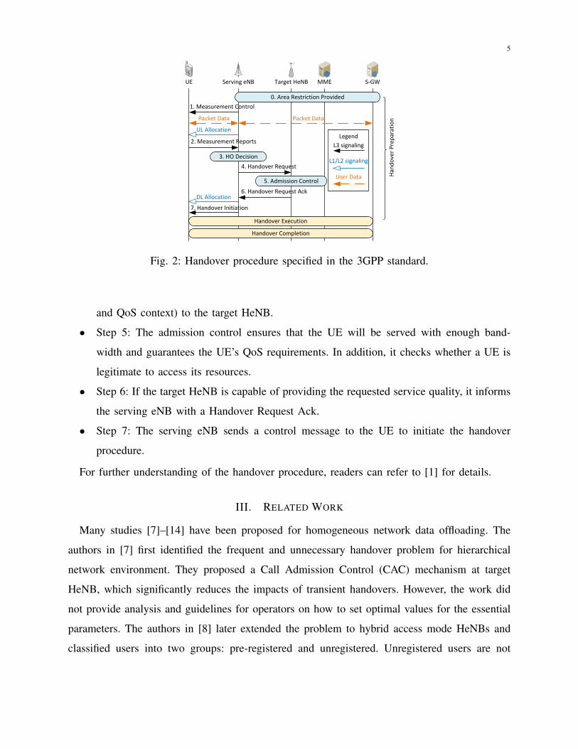
Fig. 2 shows the handover procedure specified in the 3GPP standard [1], referred to as the

baseline handover procedure in this paper. In the figure, solid lines indicate signaling messages,

and dashed lines represent user data traffic. There are three phases in the baseline procedure:

handover preparation, handover execution, and handover completion. Since the proposed algo-

rithm only involves in handover preparation phase, we elaborate the handover preparation phase

as follows:

• Step 1: The serving eNB informs the UE in which event the received signal strength should

be reported through a configuration message, and the UE keeps track of the received signal

strength of its serving cell and neighboring cells.

• Step 2: Upon a specified event1 happens, the UE sends measurement reports to the eNB.

• Step 3: The serving eNB decides whether to initiate a handover (HO) procedure to the

selected target cell based on the information received from the UE measurement reports

and the status of the neighboring cells.

• Step 4: The serving eNB sends a handover request as well as the UE context (e.g., security

1There are several measurement report triggering events defined in the 3GPP standard: event A1-A6, B1, B2, C1, and C2. Forexample, event A3 is triggered when signal level from neighbor cell becomes amount-of-offset better than serving cell. Furtherdetails can be found in [15].

5

UE Serving eNB Target HeNB MME S-GW

1. Measurement Control

UL Allocation

2. Measurement Reports

3. HO Decision

4. Handover Request

5. Admission Control

7. Handover Initiation

Handover Execution

Handover Completion

Legend

Han

do

ver

Pre

par

atio

nPacket Data Packet Data

L3 signaling

L1/L2 signaling

User Data

6. Handover Request AckDL Allocation

0. Area Restriction Provided

Fig. 2: Handover procedure specified in the 3GPP standard.

and QoS context) to the target HeNB.

• Step 5: The admission control ensures that the UE will be served with enough band-

width and guarantees the UE’s QoS requirements. In addition, it checks whether a UE is

legitimate to access its resources.

• Step 6: If the target HeNB is capable of providing the requested service quality, it informs

the serving eNB with a Handover Request Ack.

• Step 7: The serving eNB sends a control message to the UE to initiate the handover

procedure.

For further understanding of the handover procedure, readers can refer to [1] for details.

III. RELATED WORK

Many studies [7]–[14] have been proposed for homogeneous network data offloading. The

authors in [7] first identified the frequent and unnecessary handover problem for hierarchical

network environment. They proposed a Call Admission Control (CAC) mechanism at target

HeNB, which significantly reduces the impacts of transient handovers. However, the work did

not provide analysis and guidelines for operators on how to set optimal values for the essential

parameters. The authors in [8] later extended the problem to hybrid access mode HeNBs and

classified users into two groups: pre-registered and unregistered. Unregistered users are not

6

allowed to handover into femtocells so a portion of frequent handovers are efficiently avoided.

However, the frequent handover problem still exists for pre-registered users.

In [10]–[12], the authors considered Received Signal Strength (RSS) and UE’s moving speed

to reduce unnecessary handover executions. The authors in [10] designed two novel handover

algorithms based on RSS and velocity information from UEs: Velocity and Signal Handover

(VSHO) and Unequal Handover (UHO). In VSHO, a UE will handover into a femtocell if its

velocity is within the maximum handover velocity level and its RSS level is above the minimum

RSS level. As an improvement of VSHO, UHO further considers the difference of signal levels

between the eNB and the HeNB. The authors in [12] took UE mobility state and application

type into consideration, where UE mobility behaviors are classified into three states: low (0-15

km/h), medium (15-30 km/h), and high (above 30 km/h). Transient handovers caused by high

mobility UEs are avoided effectively. In [11], in addition to UE mobility state and application

type, the authors further used proactive handover procedure to reduce packet loss for real-time

services. However, in LTE networks, velocity measurement of a UE causes extra costs and may

not be accurately obtained.

Recent works [9], [13], [14] further considered UE’s signal information. In [13], the authors

proposed Double Threshold Algorithm (DTA) which uses two thresholds of Signal to Interference

and Noise Ratio (SINR) to determine whether a handover procedure should be performed.

Because DTA heavily depends on accurate measurement of SINR, serious interference in densely-

deployed metropolitan areas will cause inaccurate measurements and makes it ineffective in those

areas. In [9], the authors proposed a novel Reducing Handover Cost (RHC) mechanism in that

femtocell-to-macrocell handover requests are delayed for a period of time when UEs move out

of a femtocell. The work reduces signaling cost caused by transient handovers. However, RHC

may not have the desired outcome if the HeNBs are not in close proximity to each other. Our

recent work [14] proposes a threshold offloading algorithm considering the trade-off between

network signaling overhead and femtocell offloading capability. The algorithm significantly

reduces signaling overhead at minor cost of femtocell offloading capability. However, the work

did not consider how to select an optimal threshold value for the trade-off.

There are many studies on heterogeneous network data offloading, but we only list some

representative ones since our focus is on homogeneous network data offloading. A system called

Wiffler proposed in [16] exploits the delay tolerance of content and the contacts with fixed Access

7

Points (APs). Wiffler predicts future encounters with APs and defers data transmission only if the

transfer can be finished within the application’s tolerable threshold and reduce cellular data usage.

The work [17] proposes to use cognitive radio techniques to offload mobile traffic to wireless

APs, where the trade-off between optimal mobile traffic offloading and energy consumption

was studied. The scheme is proved to work well and can save at least 50% energy of base

stations. The authors in [18] conducted quantitative studies on the benefit of Wi-Fi offloading

with respect to network operators and mobile users. They collected trace data for two and a half

weeks from Seoul, Korea, and analyzed Wi-Fi availability. The results reveal that non-delayed

Wi-Fi offloading could already relieve a large portion of cellular data traffic, and confirm that

delayed Wi-Fi offloading has even more promising potential.

IV. PROPOSED THRESHOLD OFFLOADING (TO)

The transient handover consists of two parts: macrocell-to-femtocell and femtocell-to-macrocell

handover. The proposed Threshold Offloading (TO) is employed at the serving eNB to prevent un-

desired macrocell-to-femtocell transient handovers, and so the following femtocell-to-macrocell

handovers are also prevented.

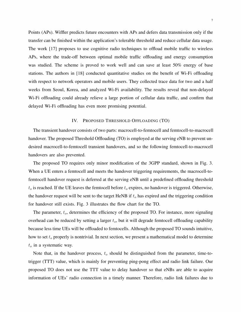
The proposed TO requires only minor modification of the 3GPP standard, shown in Fig. 3.

When a UE enters a femtocell and meets the handover triggering requirements, the macrocell-to-

femtocell handover request is deferred at the serving eNB until a predefined offloading threshold

to is reached. If the UE leaves the femtocell before to expires, no handover is triggered. Otherwise,

the handover request will be sent to the target HeNB if to has expired and the triggering condition

for handover still exists. Fig. 3 illustrates the flow chart for the TO.

The parameter, to, determines the efficiency of the proposed TO. For instance, more signaling

overhead can be reduced by setting a larger to, but it will degrade femtocell offloading capability

because less time UEs will be offloaded to femtocells. Although the proposed TO sounds intuitive,

how to set to properly is nontrivial. In next section, we present a mathematical model to determine

to in a systematic way.

Note that, in the handover process, to should be distinguished from the parameter, time-to-

trigger (TTT) value, which is mainly for preventing ping-pong effect and radio link failure. Our

proposed TO does not use the TTT value to delay handover so that eNBs are able to acquire

information of UEs’ radio connection in a timely manner. Therefore, radio link failures due to

8

UE Serving eNB Target HeNB MME S-GW

1. Measurement Control

UL Allocation

2. Measurement Reports

3. HO Decision

4. Handover Request

5. Admission Control

7. Handover Initiation

Handover Execution

Handover Completion

Legend

Han

do

ver

Pre

par

atio

n

Packet Data Packet Data

L3 signaling

L1/L2 signaling

User Data

6. Handover Request AckDL Allocation

0. Area Restriction Provided

Pro

po

sed

TO

alg

ori

thm

to expires?

HO condition still exists?

Clear timer to

and Drop HO Request

Start timer to

Clear timer to

YESNO

NO

YES

Fig. 3: The proposed TO algorithm.

the delayed handover process are avoided.

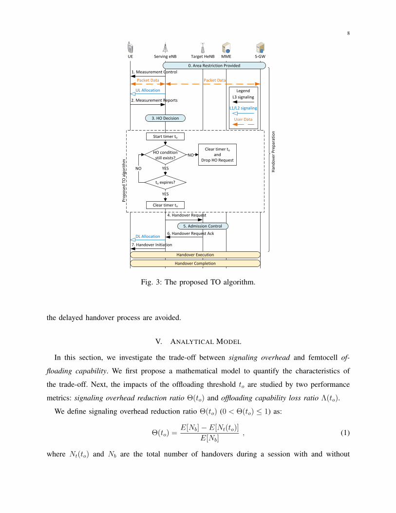
V. ANALYTICAL MODEL

In this section, we investigate the trade-off between signaling overhead and femtocell of-

floading capability. We first propose a mathematical model to quantify the characteristics of

the trade-off. Next, the impacts of the offloading threshold to are studied by two performance

metrics: signaling overhead reduction ratio Θ(to) and offloading capability loss ratio Λ(to).

We define signaling overhead reduction ratio Θ(to) (0 < Θ(to) ≤ 1) as:

Θ(to) =E[Nb]− E[Nt(to)]

E[Nb], (1)

where Nt(to) and Nb are the total number of handovers during a session with and without

9

TO, respectively. Θ(to) indicates at what percentage the proposed TO reduces total number

of handovers in a session. The higher Θ(to) is, the better the TO performs. Next, we define

offloading capability loss ratio Λ(to) (0 < Λ(to) ≤ 1) as:

Λ(to) =E[Tt(to)]

E[Tb], (2)

where Tt(to) and Tb are the total time that the session is served in femtocell with and without

TO, respectively. No assumptions made on traffic types or traffic distributions, we use time ratio

to represent the possibility that a UE’s session can be served by femtocells. Since the TO will

reduce the amount of time offloaded to femtocell during a session, Λ(to) indicates how much

offloading capability the TO can remain compared to the baseline scheme in 3GPP standard.

There is an inverse relationship between the two performance metrics, so our design goal is

to find an optimal to such that it can bring Θ(to) and Λ(to) to their possible maxima.

The radio coverage areas of femtocells overlapped with a macrocell may be continuous or

discontinuous. The difference between them is that, in discontinuous case, a UE can be at most

under one femtocell coverage, therefore there is only one target HeNB to handover. While in

continuous case, a UE can be under multiple femtocell coverage, and there are multiple target

HeNBs, which complicates UEs’ measurement reporting and handover decision. In this study,

we first consider the discontinuous case and leave the continuous one as our future work.

Because the cell shape (e.g. hexagonal or circular), the cell size, UE moving speed, and their

moving direction are hard to be characterized, in this paper, the mobility behavior of a UE is

modeled by the length of Cell Residence Time (CRT). This is commonly adopted in previous

studies [9], [19]. In our analytical model, when a UE travels in the macrocell, it alternately

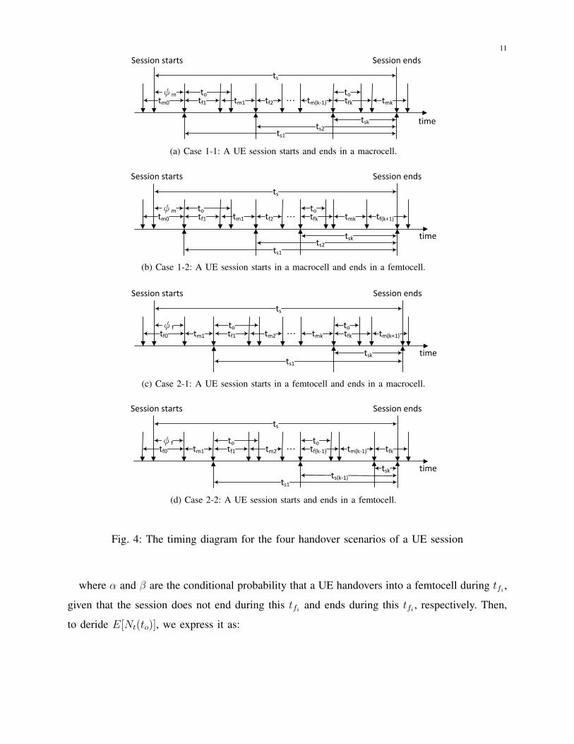
stays in the macrocell and the femtocells. A UE’s session can be categorized into four cases, as

shown in Fig. 4. In Fig. 4a, a UE’s session starts and ends in a macrocell. In Fig. 4b, a UE’s

session starts in a macrocell but ends in a femtocell. Fig. 4c shows that a UE’s session starts in

a femtocell and ends in a macrocell. A UE’s session starts and ends in a femtocell is depicted

in Fig. 4d.

During a UE’s session, for i ≥ 1, the ith CRT in a macrocell is denoted by tmi and the ith

CRT in a femtocell is denoted by tfi . For i = 0, tm0 refers to previous macrocell residence time

in which a session starts, and the same for tf0 . Next, we list the assumptions in our analysis:

10

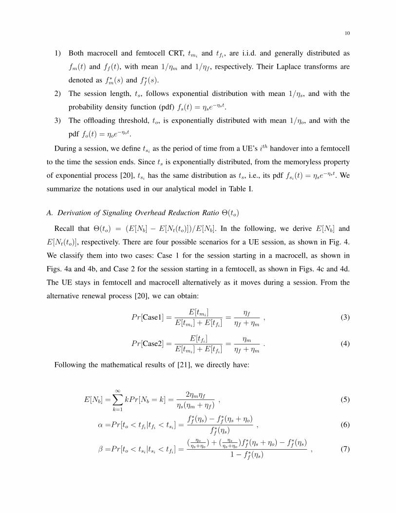
1) Both macrocell and femtocell CRT, tmi and tfi , are i.i.d. and generally distributed as

fm(t) and ff (t), with mean 1/ηm and 1/ηf , respectively. Their Laplace transforms are

denoted as f ∗m(s) and f ∗f (s).

2) The session length, ts, follows exponential distribution with mean 1/ηs, and with the

probability density function (pdf) fs(t) = ηse−ηst.

3) The offloading threshold, to, is exponentially distributed with mean 1/ηo, and with the

pdf fo(t) = ηoe−ηot.

During a session, we define tsi as the period of time from a UE’s ith handover into a femtocell

to the time the session ends. Since ts is exponentially distributed, from the memoryless property

of exponential process [20], tsi has the same distribution as ts, i.e., its pdf fsi(t) = ηse−ηst. We

summarize the notations used in our analytical model in Table I.

A. Derivation of Signaling Overhead Reduction Ratio Θ(to)

Recall that Θ(to) = (E[Nb] − E[Nt(to)])/E[Nb]. In the following, we derive E[Nb] and

E[Nt(to)], respectively. There are four possible scenarios for a UE session, as shown in Fig. 4.

We classify them into two cases: Case 1 for the session starting in a macrocell, as shown in

Figs. 4a and 4b, and Case 2 for the session starting in a femtocell, as shown in Figs. 4c and 4d.

The UE stays in femtocell and macrocell alternatively as it moves during a session. From the

alternative renewal process [20], we can obtain:

Pr[Case1] =E[tmi ]

E[tmi ] + E[tfi ]=

ηfηf + ηm

, (3)

Pr[Case2] =E[tfi ]

E[tmi ] + E[tfi ]=

ηmηf + ηm

. (4)

Following the mathematical results of [21], we directly have:

E[Nb] =∞∑k=1

kPr[Nb = k] =2ηmηf

ηs(ηm + ηf ), (5)

α =Pr[to < tfi |tfi < tsi ] =f ∗f (ηs)− f ∗f (ηs + ηo)

f ∗f (ηs), (6)

β =Pr[to < tsi|tsi < tfi ] =( ηoηs+ηo

) + ( ηsηs+ηo

)f ∗f (ηs + ηo)− f ∗f (ηs)

1− f ∗f (ηs), (7)

11

time

ts

tfktm(k-1) tmktm1tf1tm0 …

Session starts

ψm to to

Session ends

tskts2

tf2

ts1

(a) Case 1-1: A UE session starts and ends in a macrocell.

time

ts

tmktfk tf(k+1)tm1tf1tm0 … ψm to to

tskts2

tf2

ts1

Session starts Session ends

(b) Case 1-2: A UE session starts in a macrocell and ends in a femtocell.

time

ts

tfktmk tm(k+1)tf1tm1tf0 … ψf to to

tsk

tm2

ts1

Session starts Session ends

(c) Case 2-1: A UE session starts in a femtocell and ends in a macrocell.

time

ts

tm(k-1)tf(k-1) tfktf1tm1tf0 … ψf to to

tsk

tm2

ts1

ts(k-1)

Session starts Session ends

(d) Case 2-2: A UE session starts and ends in a femtocell.

Fig. 4: The timing diagram for the four handover scenarios of a UE session

where α and β are the conditional probability that a UE handovers into a femtocell during tfi ,

given that the session does not end during this tfi and ends during this tfi , respectively. Then,

to deride E[Nt(to)], we express it as:

12

TABLE I: List of Parameters

ParameterSession length tsFemtocell residence time tfMacrocell residence time tmOffloading threshold toOffloading time during the sessionwith TO

Tt

Offloading time during the sessionwithout TO

Tb

Total number of handovers during thesession with TO

Nt

Total number of handovers during thesession without TO

Nb

Number of macrocell-to-femtocellcrossings during the session

Nf

Number of femtocell-to-macrocellcrossings during the session

Nm

Number of macrocell-to-femtocellhandovers during the session

Nh

Residual life of macrocell residencetime

ψm

Residual life of femtocell residencetime

ψf

Probability density function of ts fs(t)Probability density function of tf ff (t)Probability density function of tm fm(t)Probability density function of to fo(t)Mean session length 1/ηsMean femtocell residence time 1/ηfMean macrocell residence time 1/ηmMean offloading threshold 1/ηo

E[Nt(to)]

=Pr[Case1]E[Nt(to)|Case1] + Pr[Case2]E[Nt(to)|Case2] . (8)

Let Nf and Nm be the total number of macrocell-to-femtocell crossings during ts and the

13

total number of femtocell-to-macrocell corssings during ts, respectively, where Nf +Nm = Nb.

Case 1-1: The number of cell crossings is even, i.e., N1,b = 2i, ∀i ∈ N>0, and Nf = Nm =N1,b

2. For Case 1-1, thus, we have:

E[Nt(to)|Case1-1]

=∞∑i=1

i∑k=0

(i+ k)Pr[Nt(to) = i+ k|N1,b = 2i]Pr[N1,b = 2i]

=∞∑i=1

i∑k=0

[(i+ k)

(i

k

)αk(1− α)i−k]Pr[N1,b = 2i]

=∞∑i=1

[(1 + α)i](ηmηs

)f ∗f (ηs)[1− f ∗m(ηs)]2[f ∗m(ηs)f

∗f (ηs)]

i−1

=ηmf

∗f (ηs)[1− f ∗m(ηs)]

2(1 + α)

ηs(1− f ∗m(ηs)f ∗f (ηs))2. (9)

Case 1-2: The number of cell crossings is odd, i.e., N1,b = 2i+ 1, ∀i ∈ N, Nf =N1,b+1

2and

Nm =N1,b−1

2. For Case 1-2, thus, we have:

E[Nt(to)|Case1-2]

=∞∑i=0

[β +

i∑k=0

(i+ k)Pr[Nt(to) = i+ k|N1,b = 2i+ 1]]

× Pr[N1,b = 2i+ 1]

=∞∑i=0

(β +

i∑k=0

(i+ k)

(i

k

)αk(1− α)i−k

)Pr[N1,b = 2i+ 1]

=∞∑i=0

[(1 + α)i+ β](ηmηs

)[1− f ∗f (ηs)][1− f ∗m(ηs)][f∗m(ηs)f

∗f (ηs)]

i

=ηm[1− f ∗f (ηs)][1− f ∗m(ηs)][β + (1 + α− β)f ∗m(ηs)f

∗f (ηs)]

ηs(1− f ∗m(ηs)f ∗f (ηs))2. (10)

Case 2-1: The number of cell crossings is odd, i.e., N2,b = 2i+ 1, ∀i ∈ N, Nf =N2,b−1

2and

14

Nm =N2,b+1

2. For Case 2-1, thus, we have:

E[Nt(to)|Case2-1]

=∞∑i=0

i∑k=0

(i+ 1 + k)Pr[Nt(to) = i+ k|N2,b = 2i+ 1]

× Pr[N2,b = 2i+ 1]

=∞∑i=0

i∑k=0

[(i+ 1 + k)

(i

k

)αk(1− α)i−k]Pr[N2,b = 2i+ 1]

=∞∑i=1

[1 + (1 + α)i](ηfηs

)[1− f ∗f (ηs)][1− f ∗m(ηs)][f∗m(ηs)f

∗f (ηs)]

i

=ηf [1− f ∗f (ηs)][1− f ∗m(ηs)][1 + αf ∗m(ηs)f

∗f (ηs)]

ηs(1− f ∗m(ηs)f ∗f (ηs))2. (11)

Case 2-2: The number of cell crossings is even, i.e., N2,b = 2i, ∀i ∈ N>0, and Nf = Nm =N2,b

2. For Case 2-2, thus, we have:

E[Nt(to)|Case2-2]

=∞∑i=1

(β +

i−1∑k=0

(i+ k)Pr[Nt(to) = i+ k|N2,b = 2i])

× Pr[N2,b = 2i]

=∞∑i=1

(β +

i−1∑k=0

(i+ k)

(i− 1

k

)αk(1− α)i−1−k

)Pr[N2,b = 2i]

=∞∑i=1

[(i+ α)i− α + β](ηfηs

)f ∗m(ηs)[1− f ∗f (ηs)]2[f ∗m(ηs)f

∗f (ηs)]

i−1

=ηff

∗m(ηs)[1− f ∗f (ηs)]

2[1 + β + (α− β)f ∗m(ηs)f∗f (ηs)]

ηs(1− f ∗m(ηs)f ∗f (ηs))2. (12)

By applying (3), (4), (9), (10), (11), and (12) into (8), we obtain:

E[Nt(to)]

=(1 + α)X1 + [1 + β + (1 + 2α− β)f ∗m(ηs)f∗f (ηs)]X2

+ [1 + β + (α− β)f ∗m(ηs)f∗f (ηs)]X3, (13)

15

where

X1 =ηfηmf

∗f (ηs)[1− f ∗m(ηs)]

2

ηs(ηf + ηm)(1− f ∗m(ηs)f ∗f (ηs))2,

X2 =ηfηm[1− f ∗f (ηs)][1− f ∗m(ηs)]

ηs(ηf + ηm)(1− f ∗m(ηs)f ∗f (ηs))2,

X3 =ηfηmf

∗f (ηs)[1− f ∗m(ηs)]

2

ηs(ηf + ηm)(1− f ∗f (ηs)f ∗m(ηs))2.

Therefore, our first performance metric Θ(to) can be obtained by:

Θ(to) =E[Nb]− E[Nt(to)]

E[Nb]=ηs + ηof

∗f (ηs + ηo)

2(ηs + ηo). (14)

B. Derivation of Offloading Capability Loss Ratio Λ(to)

Recall that Λ(to) = E[Tt(to)]/E[Tb]. We first derive E[Tb] for the baseline scheme without

TO and then E[Tt(to)] for the TO algorithm.

1) Derivation of E[Tb]: For the baseline scheme, let τ be the average residual life of tf0 during

ts, i.e., the average offloading time in tf0 . We then have:

τ =E[ψf |ts > ψf ]

=

∫∞tψf=0

∫∞ts=tψf

tψffψf (tψf )ηse−ηstsdtsdtψf

Pr[ts > ψf ]

=E[tψf e

−ηstψf ]

f ∗ψf (ηs). (15)

Let σ be the average age for tfi during ts, where the session ends in this tfi , i.e., the average

offloading time in the last tfi . According to the residual life theorem [20], we have:

σ = τ . (16)

Let ξ be the average offloading time in tfi , where the session does not start or end in this tfi .

16

We then have:

ξ =E[tf |ts > tf ]

=

∫∞tf=0

∫∞ts=tf

tfff (tf )ηse−ηstsdtsdtf

Pr[ts > tf ]

=E[tfe

−ηstf ]

f ∗f (ηs). (17)

Again, E[Tb] can be derived from the four scenarios and be expressed as:

E[Tb] = Pr[Case1]E[Tb|Case1] + Pr[Case2]E[Tb|Case2] . (18)

Case 1-1: Given N1,b = 2i, ∀i ∈ N>0, Nf = Nm = i, the total offloading time during ts is∑ij=1 tfj . Thus, we have:

E[Tb|Case1-1]

=∞∑i=1

E[(i∑

j=1

tfj)|N1,b = 2i]Pr[N1,b = 2i]

=∞∑i=1

iξ(ηmηs

)f ∗f (ηs)[1− f ∗m(ηs)]2[f ∗m(ηs)f

∗f (ηs)]

i−1

=ηmf

∗f (ηs)[1− f ∗m(ηs)]

2ξ

ηs(1− f ∗m(ηs)f ∗f (ηs))2. (19)

Case 1-2: Given N1,b = 2i + 1, ∀i ∈ N, Nf = i + 1 and Nm = i, the total offloading time

during ts is (∑i

j=1 tfj) + tsi+1. Thus, we have:

E[Tb|Case1-2]

=∞∑i=0

E[(i∑

j=1

tfj) + tsi+1|N1,b = 2i+ 1]Pr[N1,b = 2i+ 1]

=∞∑i=1

(iξ + σ)(ηmηs

)[1− f ∗f (ηs)][1− f ∗m(ηs)][f∗m(ηs)f

∗f (ηs)]

i

=ηm[1− f ∗f (ηs)][1− f ∗m(ηs)][σ + (ξ − σ)f ∗m(ηs)f

∗f (ηs)]

ηs(1− f ∗m(ηs)f ∗f (ηs))2. (20)

Case 2-1: Given N2,b = 2i + 1, ∀i ∈ N, Nf = i and Nm = i + 1, the total offloading time

17

during ts is ψf +∑i

j=1 tfj . Thus, we have:

E[Tb|Case2-1]Pr[Case2-1]

=∞∑i=0

E[ψf +i∑

j=1

tfj |N2,b = 2i+ 1]Pr[N2,b = 2i+ 1]

=∞∑i=1

(τ + iξ)(ηfηs

)[1− f ∗f (ηs)][1− f ∗m(ηs)][f∗m(ηs)f

∗f (ηs)]

i

=ηf [1− f ∗f (ηs)][1− f ∗m(ηs)][τ + (ξ − τ)f ∗m(ηs)f

∗f (ηs)]

ηs(1− f ∗m(ηs)f ∗f (ηs))2. (21)

Case 2-2: Given Nb = 2i, ∀i ∈ N>0, Nf = Nm = i, the total offloading time during ts is

ψf + (∑i−1

j=1 tfj) + tsi . Thus, we have:

E[Tb|Case2-2]Pr[Case2-2]

=∞∑i=1

E[ψf + (i−1∑j=1

tfj) + tsi |N2,b = 2i]Pr[N2,b = 2i]

=∞∑i=1

[τ + (i− 1)ξ + σ](ηfηs

)f ∗m(ηs)[1− f ∗f (ηs)]2

× [f ∗m(ηs)f∗f (ηs)]

i−1

=ηff

∗f (ηs)[1− f ∗m(ηs)]

2[τ + σ + (ξ − τ − σ)f ∗m(ηs)f∗f (ηs)]

ηsηf (1− f ∗m(ηs)f ∗f (ηs))2. (22)

By applying (3), (4), (19), (20), (21), and (22) into (18), we obtain:

E[Tb]

=ξX1 + [τ + σ + (2ξ − τ − σ)f ∗m(ηs)f∗f (ηs)]X2

+ [τ + σ + (ξ − τ − σ)f ∗m(ηs)f∗f (ηs)]X3, (23)

where X1, X2, and X3 are the same as those in Eq. (13).

18

2) Derivation of E[Tt(to)]: For the TO algorithm, let φ be the average offloading time for tfiduring ts, where the session does not start or end in this tfi . We then have:

φ =E[tfi − to|(to < tfi |tfi < tsi)]

=

∫ ∞to=0

∫ ∞tfi=to

∫ ∞tsi=tfi

(tfi − to)

× ηoe−ηotoff (tfi)ηse

−ηstsi

Pr[to < tfi |tfi < tsi ]Pr[tfi < tsi ]dtsidtfidto

=E[tfie

−ηstfi ] + 1ηo

(f ∗f (ηs + ηo)− f ∗f (ηs))

αf ∗f (ηs). (24)

Let ρ be the average offloading time for tfi during ts, where the session ends in this tfi . We

then have:

ρ = E[tsi − to|(to < tsi |tsi < tfi)]

=

∫ ∞to=0

∫ ∞tsi=to

∫ ∞tfi=tsi

(tsi − to)

× ηoe−ηotoηse

−ηstsiff (tfi)

Pr[to < tsi|tsi < tfi ]Pr[tsi < tfi ]dtfidtsidto

=

1ηs

+ ( 1ηo− 1

ηs)f ∗f (ηs)− E[tfie

−ηstfi ]− ηo+ηsf∗f (ηs+ηo)

ηo(ηs+ηo)

β(1− f ∗f (ηs)). (25)

Similar to the derivation of E[Tb], we express E[Tt(to)] as:

E[Tt(to)]

=Pr[Case1]E[Tt(to)|Case1] + Pr[Case2]E[Tt(to)|Case2] . (26)

Let Nh be the total number of macrocell-to-femtocell handovers during ts. E[Tt(to)] is derived

from the four scenarios as follows:

Case 1-1: Given N1,b = 2i, Nf = i, ∀i ∈ N>0, Nh is in the range 0 ≤ Nh ≤ i. The average

19

offloading time during ts is (∑i

j=0 jφPr[Nh = j]). Thus, we have:

E[Tt(to)|Case1-1]

=∞∑i=1

i∑k=0

(kφ)Pr[Nh = k|N1,b = 2i]Pr[N1,b = 2i]

=∞∑i=1

i∑k=0

[(kφ)

(i

k

)αk(1− α)i−k]Pr[N1,b = 2i]

=∞∑i=1

[αφi](ηmηs

)f ∗f (ηs)[1− f ∗m(ηs)]2[f ∗m(ηs)f

∗f (ηs)]

i−1

=ηmf

∗f (ηs)[1− f ∗m(ηs)]

2(αφ)

ηs(1− f ∗m(ηs)f ∗f (ηs))2. (27)

Case 1-2: Given N1,b = 2i+ 1, Nf = i+ 1, ∀i ∈ N, Nh is in the range 1 ≤ Nh ≤ i+ 1. The

average offloading time during ts is (βρ+∑i

j=0 jφPr[Nh = j + 1]). Thus, we have:

E[Tt(to)|Case1-2]

=∞∑i=0

(βρ+

i∑k=0

(kφ)Pr[Nh = k + 1|N1,b = 2i+ 1])

× Pr[N1,b = 2i+ 1]

=∞∑i=0

(βρ+

i∑k=0

(kφ)

(i

k

)αk(1− α)i−k

)× Pr[N1,b = 2i+ 1]

=∞∑i=0

[αφi+ βρ](ηmηs

)[1− f ∗f (ηs)][1− f ∗m(ηs)]

× [f ∗m(ηs)f∗f (ηs)]

i

=ηm[1− f ∗f (ηs)][1− f ∗m(ηs)][βρ+ (αφ− βρ)f ∗m(ηs)f

∗f (ηs)]

ηs(1− f ∗m(ηs)f ∗f (ηs))2. (28)

Case 2-1: Given N2,b = 2i+ 1, Nf = i, ∀i ∈ N, Nh is in the range 0 ≤ Nh ≤ i. The average

20

offloading time during ts is (τ +∑i

j=0 jφPr[Nh = j]). Thus, we have:

E[Tt(to)|Case2-1]

=∞∑i=0

(τ +

i∑k=0

(kφ)Pr[Nh = k|N2,b = 2i+ 1])

× Pr[N2,b = 2i+ 1]

=∞∑i=0

(τ +

i∑k=0

(kφ)

(i

k

)αk(1− α)i−k

)× Pr[N2,b = 2i+ 1]

=∞∑i=0

[τ + αφi](ηfηs

)[1− f ∗f (ηs)][1− f ∗m(ηs)][f∗m(ηs)f

∗f (ηs)]

i

=ηf [1− f ∗f (ηs)][1− f ∗m(ηs)][τ + (αφ− τ)f ∗m(ηs)f

∗f (ηs)]

ηs(1− f ∗m(ηs)f ∗f (ηs))2. (29)

Case 2-2: Given N2,b = 2i, Nf = i, ∀i ∈ N>0, Nh is in the range 1 ≤ Nh ≤ i. The average

offloading time during ts is (τ + βρ+∑i−1

j=0 jφPr[Nh = j + 1]). Thus, we have:

E[Tt(to)|Case2-2]

=∞∑i=1

(τ + βρ+

i−1∑k=0

(kφ)Pr[Nh = k + 1|N2,b = 2i])Pr[N2,b = 2i]

=∞∑i=1

(τ + βρ+

i−1∑k=0

(kφ)

(i− 1

k

)αk(1− α)i−1−k

)Pr[N2,b = 2i]

=∞∑i=1

[τ + βρ+ αφ(i− 1)](ηfηs

)f ∗m(ηs)[1− f ∗f (ηs)]2[f ∗m(ηs)f

∗f (ηs)]

i−1

=ηmf

∗m(ηs)[1− f ∗f (ηs)]

2[τ + βρ]

ηs(1− f ∗m(ηs)f ∗f (ηs))2

+ηmf

∗m(ηs)[1− f ∗f (ηs)]

2[(αφ− τ − βρ)f ∗m(ηs)f∗f (ηs)]

ηs(1− f ∗m(ηs)f ∗f (ηs))2. (30)

21

By applying (3), (4), (27), (28), (29), and (30) into (26), we have:

E[Tt(to)]

=αφX1 + [τ + βρ+ (2αφ− τ − βρ)f ∗m(ηs)f∗f (ηs)]X2

+ [τ + βρ+ (αφ− τ − βρ)f ∗m(ηs)f∗f (ηs)]X3, (31)

where X1, X2, and X3 are the same as those in Eq. (13).

Therefore, our second performance metric Λ(to) can be obtained by:

Λ(to) =E[Tt(to)]

E[Tb]=ηfηo − ηf (ηs + ηo)f

∗f (ηs) + ηfηsf

∗f (ηs + ηo) + η2s(ηs + ηo)Y2

ηs(ηs + ηo)(ηfY1 + 2ηsY2). (32)

where Y1 = E[tfe−ηstf ] and Y2 = E[tψf e

−ηstψf ] .

VI. SIMULATION AND NUMERICAL RESULTS

In this section, we provide numerical results for the analysis presented in Section V. The

analysis is validated through extensive simulations by using ns-2 [22], version 2.35. In addition,

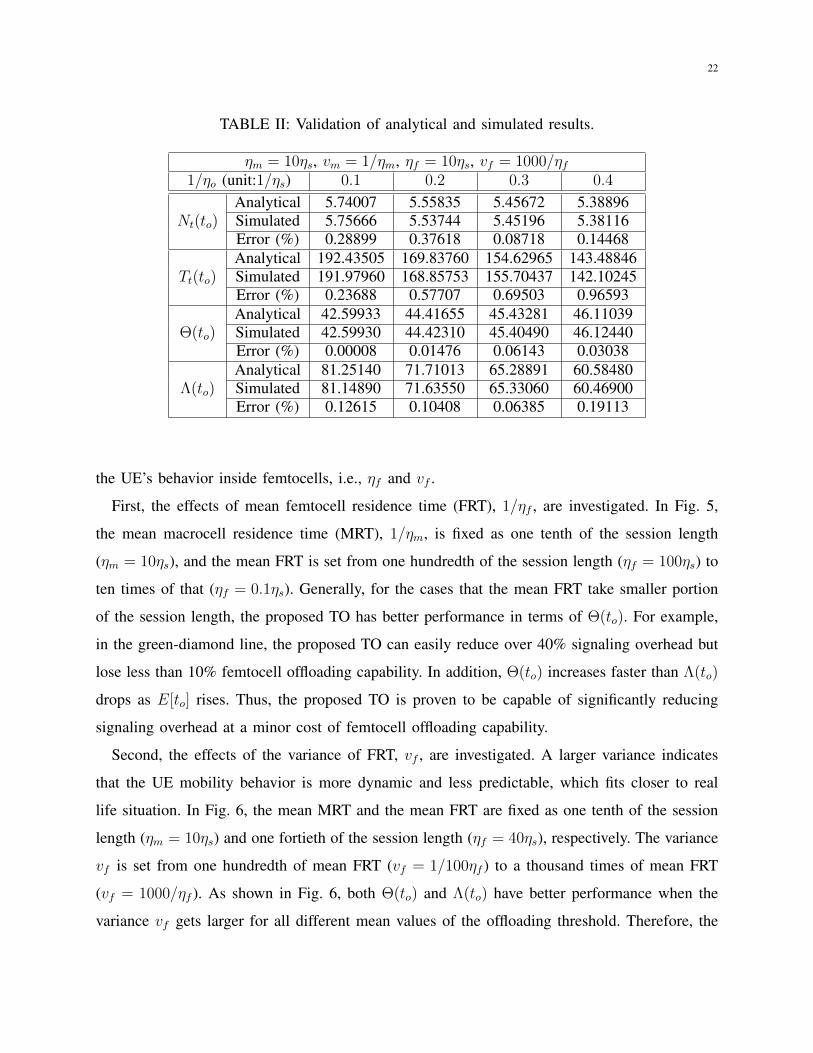
the errors between the analytical and simulated results are verified to fall within one percent.

Due to page limitation, we only show one table of our results, Table II.

The two performance metrics, i.e., (14) and (32), can be organized into a meaningful form only

if f ∗f (s) and f ∗m(s) have closed-form solutions. Thus, we choose to apply Gamma distribution

for both femtocell residence time and macrocell residence time because the Gamma distribution

has two characteristics: (1) it is a more general kind of distribution and can approximate many

other distributions, and (2) a closed-form Laplace transform solution for it exists. Also, the

Gamma distribution has been commonly adopted in many previous papers (e.g. [19], [23]) to

study various UE mobility behaviors.

Then, we observe that two factors affects the performance of our proposed TO: the effects of

UE mobility and the session length. Their impact are investigated and the results are illustrated

in Figs. 5–7.

A. Effects of UE Mobility

As shown in Eqs. (14) and (32), the UE’s behavior inside the macrocell (ηm and vm) have no

impacts on the two performance metrics, the effects of UE mobility can be simply reflected by

22

TABLE II: Validation of analytical and simulated results.

ηm = 10ηs, vm = 1/ηm, ηf = 10ηs, vf = 1000/ηf1/ηo (unit:1/ηs) 0.1 0.2 0.3 0.4

Nt(to)Analytical 5.74007 5.55835 5.45672 5.38896Simulated 5.75666 5.53744 5.45196 5.38116Error (%) 0.28899 0.37618 0.08718 0.14468

Tt(to)Analytical 192.43505 169.83760 154.62965 143.48846Simulated 191.97960 168.85753 155.70437 142.10245Error (%) 0.23688 0.57707 0.69503 0.96593

Θ(to)Analytical 42.59933 44.41655 45.43281 46.11039Simulated 42.59930 44.42310 45.40490 46.12440Error (%) 0.00008 0.01476 0.06143 0.03038

Λ(to)Analytical 81.25140 71.71013 65.28891 60.58480Simulated 81.14890 71.63550 65.33060 60.46900Error (%) 0.12615 0.10408 0.06385 0.19113

the UE’s behavior inside femtocells, i.e., ηf and vf .

First, the effects of mean femtocell residence time (FRT), 1/ηf , are investigated. In Fig. 5,

the mean macrocell residence time (MRT), 1/ηm, is fixed as one tenth of the session length

(ηm = 10ηs), and the mean FRT is set from one hundredth of the session length (ηf = 100ηs) to

ten times of that (ηf = 0.1ηs). Generally, for the cases that the mean FRT take smaller portion

of the session length, the proposed TO has better performance in terms of Θ(to). For example,

in the green-diamond line, the proposed TO can easily reduce over 40% signaling overhead but

lose less than 10% femtocell offloading capability. In addition, Θ(to) increases faster than Λ(to)

drops as E[to] rises. Thus, the proposed TO is proven to be capable of significantly reducing

signaling overhead at a minor cost of femtocell offloading capability.

Second, the effects of the variance of FRT, vf , are investigated. A larger variance indicates

that the UE mobility behavior is more dynamic and less predictable, which fits closer to real

life situation. In Fig. 6, the mean MRT and the mean FRT are fixed as one tenth of the session

length (ηm = 10ηs) and one fortieth of the session length (ηf = 40ηs), respectively. The variance

vf is set from one hundredth of mean FRT (vf = 1/100ηf ) to a thousand times of mean FRT

(vf = 1000/ηf ). As shown in Fig. 6, both Θ(to) and Λ(to) have better performance when the

variance vf gets larger for all different mean values of the offloading threshold. Therefore, the

23

0 0.1 0.2 0.3 0.4 0.5(A) E[to] (unit: 1/ηs)

0

12.5

25

37.5

50

Θ(t

o)(%

)

Math, ηf = 100ηs Math, ηf = 10ηs Math, ηf = ηs Math, ηf = 0.1ηs

0 0.1 0.2 0.3 0.4(B) E[to] (unit: 1/ηs)

53

62.5

75

87.5

100

Λ(t

o)(%

)

(0.04040, 40.24250)

(0.04040, 90.01340)

Sim., ηf = 100ηs Sim., ηf = 10ηs Sim., ηf = ηs Sim., ηf = 0.1ηs

Fig. 5: The effects of mean femtocell residence time ηf on Θ(to) and Λ(to) (ηm = 10ηs).

(A) Variance vf (unit: 1/ηf )0 200 400 600 800 1000

Θ(t

o)(%

)

0

12.5

25

37.5

50

Math, ηo = 1000ηs Math, ηo = 100ηs Math, ηo = 10ηs Math, ηo = ηs

(B) Variance vf (unit: 1/ηf )0 200 400 600 800 1000

Λ(t

o)(%

)

0

25

50

75

100

Sim., ηo = 1000ηs Sim., ηo = 100ηs Sim., ηo = 10ηs Sim., ηo = ηs

Fig. 6: The effects of variance of femtocell residence time vf on Θ(to) and Λ(to) (ηm = 10ηs,ηf = 40ηs).

proposed TO is considered effective against various UE mobility behaviors in real life.

B. Effects of Session Length

In Fig. 7, the mean MRT and the mean FRT are fixed as 60 and 15 seconds, respectively.

The mean session length is set from 0 to 150 seconds (i.e., 10/ηf ). We observe that the mean

session length has prominent effects on the two performance metrics only when it is smaller than

the mean FRT, i.e., ηs > ηf , while it tends to be less perceivable when ηs < ηf . In the case of

24

(A) E[ts] (unit: 1/ηf )0 2 4 6 8 10

Θ(t

o)(%

)

44

46

48

50

Math, ηo = 1000ηs Math, ηo = 100ηs Math, ηo = 10ηs Math, ηo = ηs

(B) E[ts] (unit: 1/ηf )0 2 4 6 8 10

Λ(t

o)(%

)

40

55

70

85

100

Sim., ηo = 1000ηs Sim., ηo = 100ηs Sim., ηo = 10ηs Sim., ηo = ηs

Fig. 7: The effects of mean session length ηs on Θ(to) and Λ(to) (1/ηm = 60s, 1/ηf = 15s).

ηs > ηf , Θ(to) decreases when the session length increases. It is because the offloading threshold

takes smaller proportion of the session length when ts gets larger. On the other hand, for ηs > ηf ,

Λ(to) increases when the session length increases because the offloading time lengthens along

with the session length. Thus, depending on whether the mean session length is smaller than the

mean FRT, the significance of the session length can be determined. Overall, for ηs > ηf , both

UE mobility behaviors and the session length have impacts on the two performance metrics,

while the effects of UE mobility dominate for the case of ηs < ηf .

VII. OPTIMAL TO ALGORITHM

A. Determination of Optimal Offloading Threshold

It is of high priority for network operators to select a proper offloading threshold to, such

that the TO algorithm is efficient. A large offloading threshold to will reduce massive network

signaling overhead but sacrifice femtocell offloading capability. On the other hand, a small

offloading threshold to reserves more femtocell offloading capability but costs higher network

signaling overhead. Recall that to is an exponential random variable, and our goal is to find

the optimal mean offloading threshold, aka the optimal distribution, such that Θ(to) and Λ(to)

together achieve maximum. From Eqs. (14) and (32), both Θ(to) and Λ(to) are functions of ηo,

thus we formulate the objective function as:

25

0 50 100 150 200(A) E[to] (unit: second)

100

110

120

130

140

150

f(η

o)(%

)

ηf = 20ηsηf = 10ηsηf = 5ηsηf = 2.5ηs

0 5 10 15 20 25100

110

120

130

140

150(2.11170, 140.09716)

(4.60375, 133.61637)

(9.67217, 124.53416)

(18.41140, 113.73035)

Fig. 8: Determination of the optimal offloading threshold.

maximizeηo

f(ηo) = Θ(ηo) + Λ(ηo)

subject to 0 < ηo ≤ δ ,

(33)

where δ is the upperbound of ηo, which can be determined by operators according to their

historical statistic data, and define the optimal offloading threshold as:

E[to]∗ =

1

η∗o. (34)

Then, according to Calculus, such η∗o can be found by solving the differential equation

f′(ηo) = 0 and checking the boundary values, i.e., f(0) and f(δ). Since the closed-form

solution to the differential equation does not have a meaningful and simplified expression, we

instead acquire the answer by using MATLAB. The mean computing time for the η∗o obtained by

using a normal PC (Intel Core i5-3470 with 8G RAM) is 121.56 ms with the standard deviation

of 1.97 ms.

Fig. 8 illustrates a graphical plot of f(ηo) with 4 different settings. In this example, the session

length ts and the upperbound δ are set as 600 second and 200 second, respectively. We solve the

equation f′(ηo) = 0 and compare it with the boundary values for each line, and the maximum

values are denoted as crosses in the figure. For the green line (ηf = 10ηs), the optimal offloading

threshold E[to]∗ is computed as 4.60375, with the corresponding η∗o as 0.21721. Thus, operators

can achieve the best performance for the TO algorithm by setting the optimal η∗o .

26

Algorithm 1 Selecting an optimal offloading threshold.Input: δOutput: η∗oEnsure: η∗o ∈ (0, δ]

1: if f ′(ηo) = 0 has a real solution η′o then2: if f(δ) > f(0) then3: if f(η

′o) > f(δ) then

4: return η′o

5: else6: return f(δ)7: end if8: else9: if f(η

′o) > f(0) then

10: return η′o

11: else12: return f(0)13: end if14: end if15: else if f(δ) > f(0) then16: return δ17: else18: return 019: end if

Next, we propose an algorithm (shown as Algorithm 1) to systematically find η∗o . Algorithm 1

takes one input value: δ, which is the upperbound for ηo. Again, operators can refer to their

historical statistics on femtocell CRT and determine δ accordingly. First, Algorithm 1 checks if

f′(ηo) = 0 has a real solution, say, η′o. If no, then return the larger boundary value. Otherwise,

it compares η′o with the two boundary values, and return whichever the largest as the optiaml

offloading threshold. Note that when η∗o is returned as 0, E[to]∗ would goes to infinity. In practice,

this can be solved by just setting η∗o as an arbitrary small number.

B. Implementation Issues

To use the TO algorithm, we need to gather statistics of E[tf ], E[tm], and E[ts] in advance.

First, HeNBs can continuously collect each UE’s duration in the femtocells by observing the

time stamps when it performs handover in and handover out. The HeNBs then upload their own

E[tf ] to the eNB, which in turn will compute a combined E[tf ] from all HeNBs. Note that the

frequency for uploading E[tf ] involves the tradeoff between the precision of the TO algorithm

27

and extra signaling overhead. Second, eNBs can obtain E[tm] when HeNBs obtain E[tf ]. Last,

E[ts] can be acquired by recording the lifetime of traffic flows at the entities in the core network,

such as P-GW or Policy Charging Rule Function (PCRF) [24].

VIII. CONCLUSIONS

In this paper, we propose the TO algorithm by considering the trade-off between network

signaling overhead and femtocell offloading capability. The TO algorithm is evaluated by two

performance metrics: signaling overhead reduction ratio Θ(to) and offloading capability loss ratio

Λ(to). Our analytical model and simulation results show consistent findings that the proposed TO

algorithm is capable of significantly reducing signaling overhead against various UE mobility

behaviors while little femtocell offloading capability is compromised, particularly for UEs with

more dynamic mobility behaviors (i.e., larger vf ). Moreover, our work provides guidelines for

network operators on how to set an optimal offloading threshold to achieve the best performance.

REFERENCES

[1] 3GPP TS 36.300 V12.5.0, Evolved Universal Terrestrial Radio Access (E-UTRA) and Evolved Universal Terrestrial Radio

Access Network (E-UTRAN); Overall description; Stage 2 (Release 12), Std., Mar. 2015.

[2] “2014 Annual Report,” AT&T, Tech. Rep., 2014.

[3] “Cisco Visual Networking Index: Global Mobile Data Traffic Forecast Update 2014V2019 White Paper,” Cisco, Tech.

Rep., Feb. 2015.

[4] “Small Cell Forum,” http://www.smallcellforum.org/.

[5] V. Chandrasekhar, J. G. Andrews, and A. Gatherer, “Femtocell networks: a survey,” IEEE Commun. Mag., vol. 46, no. 9,

pp. 59–67, 2008.

[6] “Urban small cells in the real world: case studies,” Small Cell Forum, Tech. Rep., 2014.

[7] M. Z. Chowdhury, W. Ryu, E. Rhee, and Y. M. Jang, “Handover between macrocell and femtocell for UMTS based

networks,” in Proc. IEEE 11th Int’l Conf. Advanced Communication Technology, ICACT, 2009, pp. 237–241.

[8] J.-S. Kim and T.-J. Lee, “Handover in UMTS networks with hybrid access femtocells,” in Proc. IEEE 12th Int’l Conf.

Advanced Communication Technology, ICACT, vol. 1, 2010, pp. 904–908.

[9] C.-P. Lee, K.-F. Huang, P. Lin, H.-J. Su, and C.-L. Wang, “Reducing handover cost for LTE femtocell/macrocell network,”

in Proc. IEEE GLOBECOM, 2013, pp. 4988–4993.

[10] W. Shaohong, Z. Xin, Z. Ruiming, Y. Zhiwei, F. Yinglong, and Y. Dacheng, “Handover study concerning mobility in the

two-hierarchy network,” in Proc. IEEE Veh. Technol. Conf., VTC, 2009, pp. 1–5.

[11] A. Ulvan, R. Bestak, and M. Ulvan, “The study of handover procedure in LTE-based femtocell network,” in Proc. 3rd

Joint IFIP Wireless and Mobile Networking Conference, WMNC, 2010, pp. 1–6.

28

[12] H. Zhang, X. Wen, B. Wang, W. Zheng, and Y. Sun, “A novel handover mechanism between femtocell and macrocell for

LTE based networks,” in Proc. IEEE Int’l Conf.Communication Software and Networks, ICCSN, 2010, pp. 228–231.

[13] G. Yang, X. Wang, and X. Chen, “Handover control for LTE femtocell networks,” in Proc. IEEE Int’l Conf. Electronics,

Communications and Control, ICECC, 2011, pp. 2670–2673.

[14] W.-H. Chen, Y. Ren, and J.-C. Chen, “Design and analysis of a threshold offloading (TO) algorithm for LTE

femtocell/macrocell networks,” in 2016 IEEE Symposium on Computers and Communication (ISCC), to be published.

[15] 3GPP TS 36.331 V12.5.0, LTE; Evolved Universal Terrestrial Radio Access (E-UTRA); Radio Resource Control (RRC);

Protocol specification (Release 12), Std., Apr. 2015.

[16] A. Balasubramanian, R. Mahajan, and A. Venkataramani, “Augmenting mobile 3G using WiFi,” in Proc. ACM 8th int’l

Conf. Mobile systems, applications, and services, 2010, pp. 209–222.

[17] T. Han and N. Ansari, “Enabling mobile traffic offloading via energy spectrum trading,” IEEE Trans. Wireless Commun.,

vol. 13, no. 6, pp. 3317–3328, Jun. 2014.

[18] K. Lee, J. Lee, Y. Yi, I. Rhee, and S. Chong, “Mobile data offloading: How much can WiFi deliver?” IEEE/ACM Trans.

Netw., vol. 21, no. 2, pp. 536–550, 2013.

[19] R.-H. Liou, Y.-B. Lin, and S.-C. Tsai, “An investigation on LTE mobility management,” IEEE Trans. Mobile Comput.,

vol. 12, no. 1, pp. 166–176, 2013.

[20] S. M. Ross, Introduction to probability models. Academic press, 2014.

[21] H.-L. Fu, P. Lin, and Y.-B. Lin, “Reducing signaling overhead for femtocell/macrocell networks,” IEEE Trans. Mobile

Comput., vol. 12, no. 8, pp. 1587–1597, 2013.

[22] “The nework simulator - ns-2,” http://www.isi.edu/nsnam/ns/.

[23] W. Ma and Y. Fang, “Dynamic hierarchical mobility management strategy for mobile IP networks,” IEEE J. Sel. Areas

Commun., vol. 22, no. 4, pp. 664–676, 2004.

[24] 3GPP TS 23.261 V12.0.0, IP flow mobility and seamless Wireless Local Area Network (WLAN) offload; Stage 2 (Release

12), Std., Sep. 2014.