1

2

Department of Electronics Engineering

Sahand University of Technology

NMOS inverter with an n-channel enhancement-mode mosfet

with the gate connected to the drain

Farshad Gozalpoor

Professor : Dr Najafi Aghdam

winter 93

3

We will analyze the dc voltage transfer

characteristics of this inverter in this figure.

We will also define and develop the noise margin of

this digital circuit in terms of the inverter voltage

transfer curve.

We will then determine the impact of the body

effect on the dc voltage transfer curve and the

logic levels.

A transient analysis of the NMOS inverter will

determine the propagation delay time in NMOS logic

circuits.

Abstract

4

The drain current is zero.

A nonzero drain current is induced in the device.

We can see that the following condition is satisfied:

A transistor with this connection always operates in the saturation region when not in cutoff.

Diode connected transistor

5

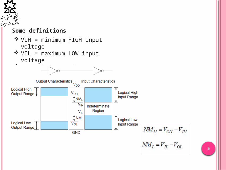
VIH = minimum HIGH input voltage VIL = maximum LOW input voltage VOH= minimum HIGH output

voltage VOL = maximum LOW output

voltage

Some definitions

6

HINT:In the following analysis, we neglect the body effect and we assume all threshold voltages are constant. These assumptions do not seriously affect the basic analysis or the inverter characteristics.

The driver is cut off and the drain currents are zero.

Assumptin:

VTC computations

M1 : Off

M2 : Sat

7

M1: Sat

M2: Sat

8

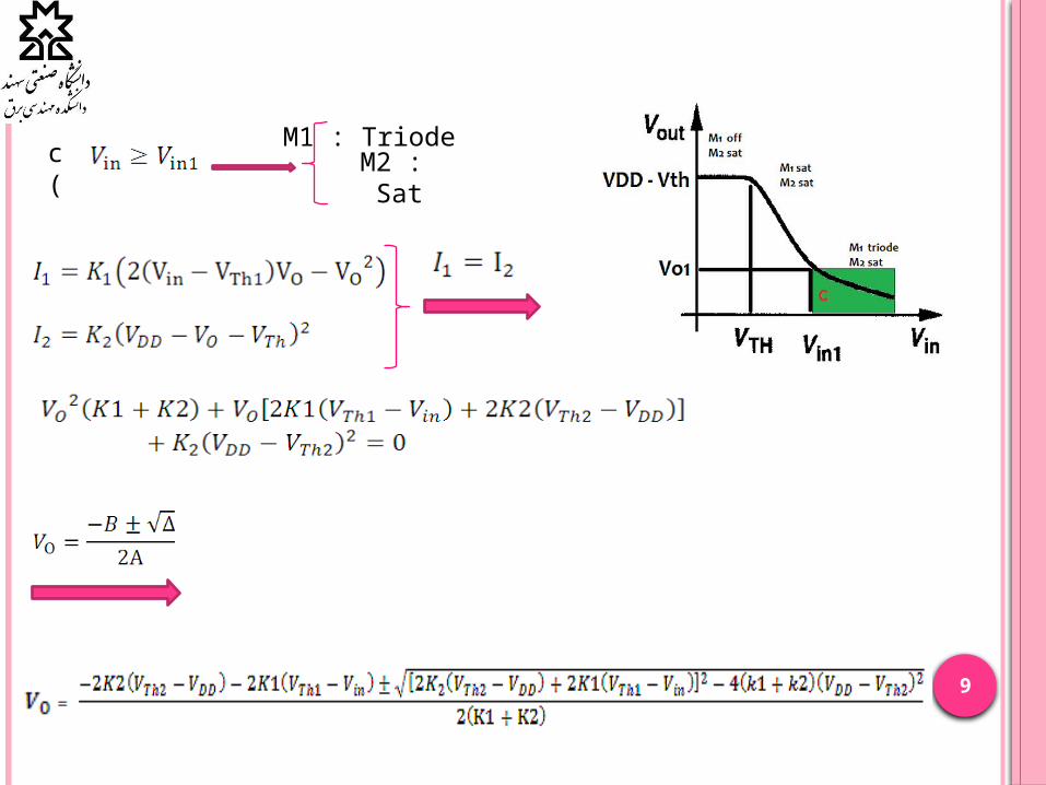
Computing Vin1 and Vo1:

9

c) M1 : Triode

M2 : Sat

10

: Assumption

Vin=1.5

K1=20

K2=10

Vth=0.41v

VO+ = 2.069VO - = 0.31

11

Computing VIH:

12

Analysis of the transient behavior of the gate

Drain diffusion capacitances of the NMOS transistors, the capacitance of the connecting wires, and the input capacitance of the fan-out gates

LC

A fast gate is built either by keeping the output capacitance small or by decreasing the on-resistance of the transistor.

13

Switching Threshold

We solve the case where the supply voltage is high so that the devices can beassumed to be velocity-saturated

1 21 1 1 2 2 2( ) ( ) 0

2 2DSATn DSATn

n DSATn M Tn n DSATn M DD Tn

V Vk V V V k V V V V

1 21 2( ) ( )

2 21

DSATn DSATnTn DD Tn

M

V VV r V V

Vr

2 , 22 2

1 1 1 , 1

n sat nn DSATn

n DSATn n sat n

W vk Vr

k V W v Where

14

For large values of VDD

1DD

M

rVV

r

It is considered to be desirable for VM to be located around the

middle of the available voltage swing.

To move VM upwards, a larger value of r is required.

Increasing the strength of the NMOS, on the other hand, moves the switching threshold closer to GND.

2 1 1 1 1

1 2 2 2 2

( / ) ( / 2)

( / ) ( / 2)n n DSATn M Tn DSATn

n n DSATn DD M Tn DSATn

W L k V V V V

W L k V V V V V

15

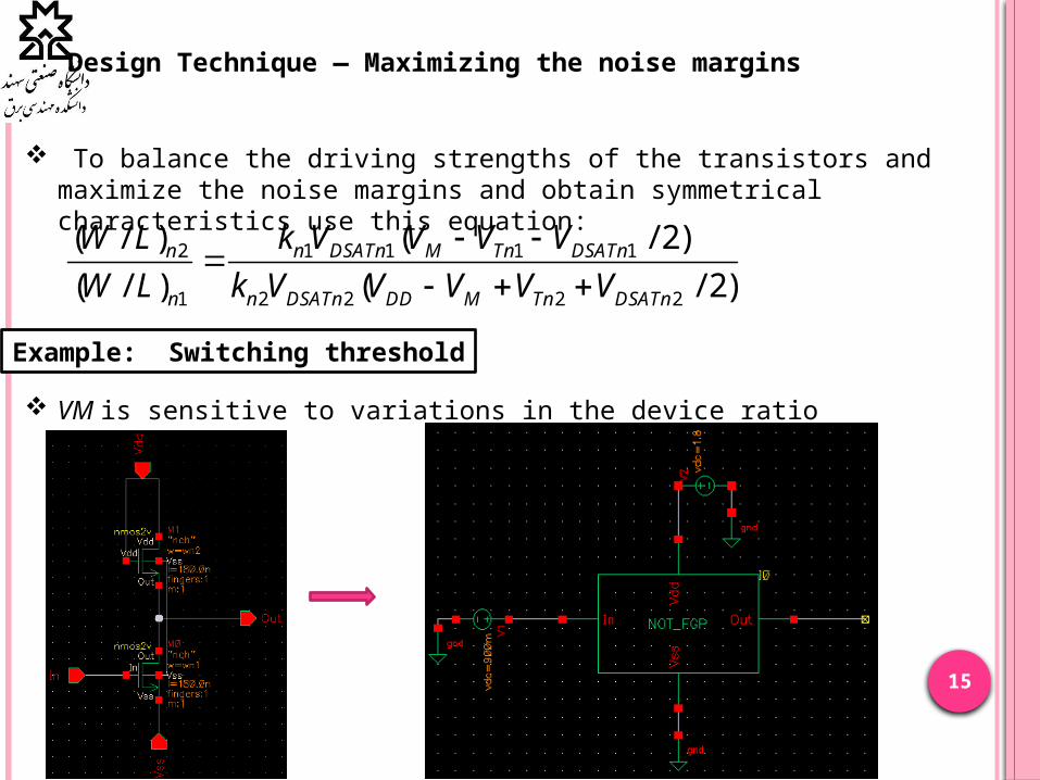
Design Technique — Maximizing the noise margins

To balance the driving strengths of the transistors and maximize the noise margins and obtain symmetrical characteristics use this equation:

2 1 1 1 1

1 2 2 2 2

( / ) ( / 2)

( / ) ( / 2)n n DSATn M Tn DSATn

n n DSATn DD M Tn DSATn

W L k V V V V

W L k V V V V V

Example: Switching threshold

VM is sensitive to variations in the device ratio

16

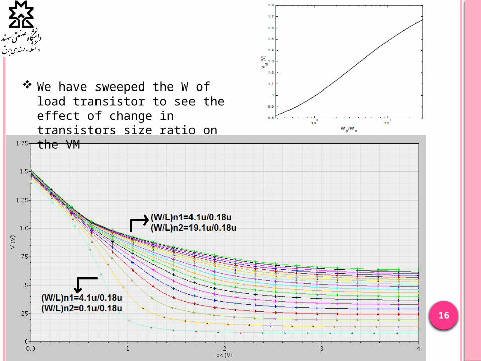
We have sweeped the W of load transistor to see the effect of change in transistors size ratio on the VM

17 This means that small variations of the ratio do not disturb the transfer characteristic that much.

18

The usage of shifting the transient region of the VTC by changing VM

19

Another example for VTC

20

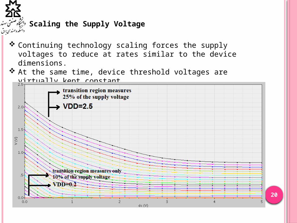
Scaling the Supply Voltage

Continuing technology scaling forces the supply voltages to reduce at rates similar to the device dimensions.

At the same time, device threshold voltages are virtually kept constant.

21

At a voltage of 0.2 V the width of the transition region measures only 10% of the supply voltage while it widens to 25% for 2.5 V

So, given this improvement in dc characteristics why do we not choose to operate all our digital circuits at these

low supply voltages?

reducing the supply voltage has a positive impact on the energy dissipation, but is detrimental to the performance on the gate.

The dc-characteristic becomes increasingly sensitive to variations in the device

parameters such as the transistor threshold, once supply voltages and intrinsic voltages become comparable.

22

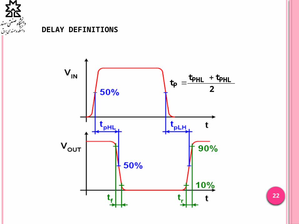
DELAY DEFINITIONS

2

ttt PHLPHL

P

23

First-Order Analysis

Integrate the capacitor (dis)charge current: i the (dis)charging current v the voltage over the capacitor v1 and v2 the initial and final voltage

Equivalent resistance when (dis)charging a capacitor:

24

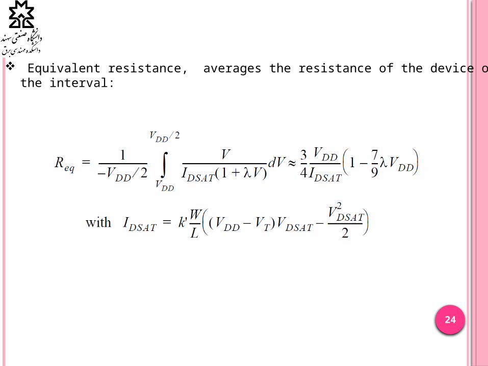
Equivalent resistance, averages the resistance of the device over the interval:

25

Example

Assume that a driver with a source resistance of 10 kW is used to drive a 10 cm long, 1 mm wide Al1 wire with total lumped capacitance for this wire equals 11 pF

The operation of this simple RC network is described by the following ordinary differential Equation:

26

When applying a step input, the transient response of this circuit is

Where:

driver lumpedR C The time to reach the 50% point: t = ln(2)t = 0.69t To get to the 90% point: t= ln(9)t = 2.2t

the propagation delay of such a network for a voltage step at the input is proportional to the time-constant of the network.

27

the propagation delay of such a network for a voltage step at the input is proportional to the time-constant of the network:

1 1(2) 0.69pHL eqn L eqn Lt R C Ln R C

20.69pLH eqn Lt R C

Example:

The overall propagation delay of the inverter:

1 2R0.69 ( )

2 2pHL pLH eqn eqn

p L

t t Rt C

Propagation Delay of a 0.25 mm Inverter

28

supply voltage equals to 2.5 V

The (W/L) ratios of the transistors to be 1.5 for the NMOS1, and 4.5 for the NMOS2.

29

make the parameters governing the delay explicit

/ 2DD Tn DSATnV V V

Propagation delay of inverter as a function of supply voltage

30

The propagation delay of a gate can be minimized in the following ways:

Reduce CL: three major factors contribute to the load capacitance: the internal diffusion capacitance of the gate itself, the interconnect capacitance, and the fanout.

Increase the W/L ratio of the transistors. This is the most powerful and effective performance optimization tool in the hands of the designer.

Increase VDD

31

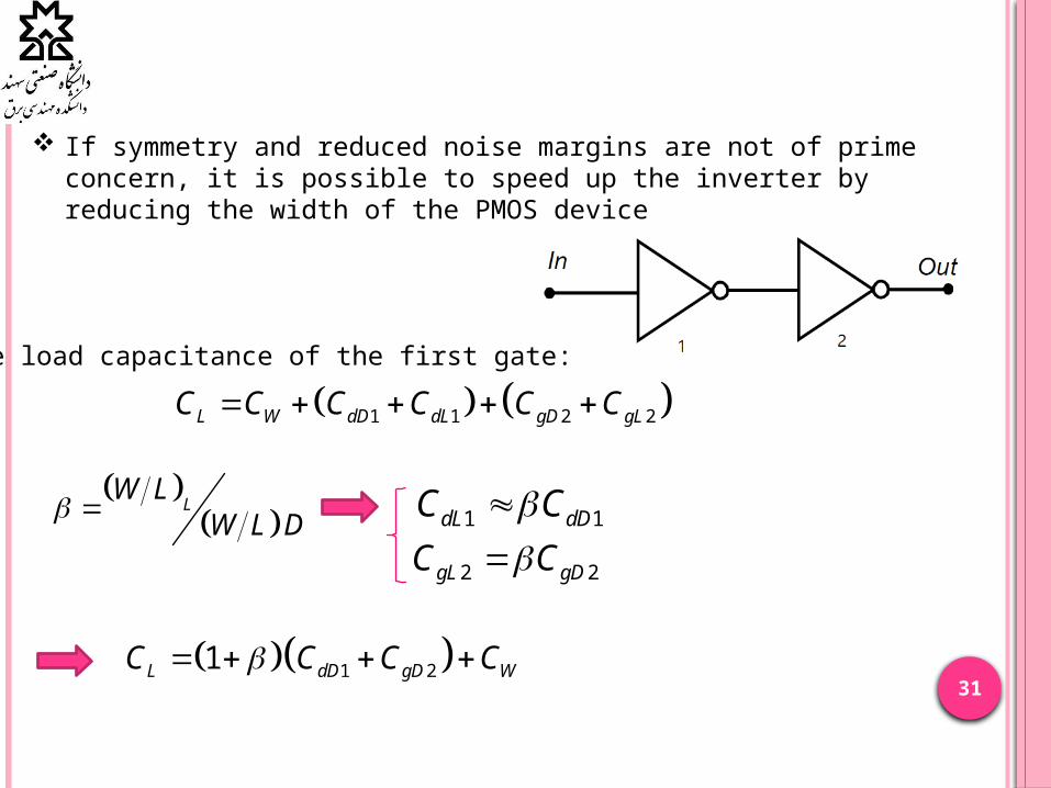
If symmetry and reduced noise margins are not of prime concern, it is possible to speed up the inverter by reducing the width of the PMOS device

The load capacitance of the first gate:

1 1 2 2L W dD dL gD gLC C C C C C

LW L

W L D 1 1dL dDC C

2 2gL gDC C

1 21L dD gD WC C C C

32

1 2

1 2

0.691

2

0.345 1 1 ,

eqLP dD gD W eqD

eqLdD gD W eqD

eqD

Rt C C C R

RrC C C R r

R

0Pt

1 2

1 Wopt

dD gD

Cr

C C

By setting:

Sizing Inverters for Performance

intL extC C C Cint is associated with the diffusion capacitances of the NMOS and PMOS

transistors as well as the gate-drain overlap (Miller) capacitance Cext is the extrinsic load capacitance

33

int

int 0int int

0.69

0.69 1 1

P eq ext

ext exteq P

t R C C

C CR C t

C C

tp0 = 0.69 ReqCint represents the delay of the inverter only loaded by its own

intrinsic capacitance (Cext = 0), and is called the intrinsic or unloaded delay

int

0

,

0.69 1 /

0.69 1 1

refiref eq

refP iref ext iref

ext extref iref P

iref iref

RC SC R

SR

t SC C SCS

C CR C t

SC SC

34

The intrinsic delay of the inverter tp0 is independent of the sizing of the gate, and determined by technology and inverter layout.

Making S infinitely large yields the maximum performance gain, eliminating the impact of external load, and reducing the delay to the intrinsic one.

Sizing A Chain of Inverters: Determining the optimum sizing of a gate when embedded in a real environment.

int

0 01 1

g

extP P P

g

C C

Ct t t f

C

g is a proportionality factor, which is only a function of technology

Delay if the inverter is function of the ratio between its external load capacitance and input capacitance. This ratio is called the effective fanout f.

35

The goal is to minimize the delay through the inverter chain

, 1, 0 0

,

, 1, ,0 , 1

1 1 ,

1 1

1 :

g j jp j p p

g j

N Ng j

p p j p g N Lj j g j

C ft t t

C

CTotal Delay t t t with C C

C

,

, 1 ,

, , 1

0

:

P

g j

g j g j

g j g j

t

C

C CA set of

C C

the optimum size of each inverter is the geometric mean of its neighbors sizes , , 1 . 1g j g j g jC C C

36

With Cg,1 and CL given:,1

0 1

NLN

g

N

p p

Cf F

C

FMinimum Delay t Nt

Choosing the Right Number of Stages in an Inverter Chain

The optimum value can be found by differentiating the minimum delay expression by the number of stages, and setting the result to 0.

1ln0

NN fF F

F f eN

For g = 0:

Optimal number of stages equals N = Ln(F) Effective fan out of each stage is set to f = 2.71828 = e

37

Optimum effective fanout f as a function of the self-loading factor g in an inverter chain

Normalized propagation delay (tp/(tpopt)

as a function of the effective fanout f for =1g.

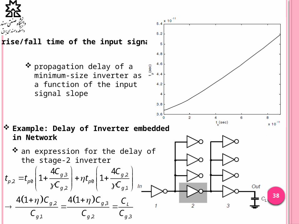
38

The rise/fall time of the input signal

propagation delay of a minimum-size inverter as a function of the input signal slope

Example: Delay of Inverter embedded in Network

an expression for the delay of the stage-2 inverter

,3 ,2,2 0 0

,2 ,1

,2 ,3

,1 ,2 ,3

4 41 1

4 1 4 1

g gp p p

g g

g g L

g g g

C Ct t t

C C

C C C

C C C

39

Power, Energy, and Energy-Delay

The power dissipation of an inverter is dominated by dynamic dissipation resulting from charging and discharging capacitances.

Dynamic Power Consumption Dynamic Dissipation due to Charging and Discharging Capacitances

2

0 0 0

DDVout

VDD VDD DD DD L L DD out L DD

dvE i t V dt V C dt C V dv C V

dt

2

0 0 0 2

DDVout L DD

C VDD out L out L out out

dv C VE i t v dt C v dt C v dv

dt

40

This means that only half of the energy supplied by the power source is stored on CL

Example: Capacitive power dissipation of inverter

the value of the load capacitance was determined to equal 6 fF

For a supply voltage of 2.5 V

2 37.5

12 65 sec

5802

dyn L DD

pLH pHL p

dyndyn

p

E C V fJ

T t t t pf

EP W

t

41

switching activity

2 2 20 1 0 1dyn L DD L DD EFF DDP C V f C V P C V f

f : maximum possible event rate of the inputs P0®1 : probability that a clock event results in a 0® 1

event at the output of the gate. CEFF = P0®1CL is called the effective capacitance and represents the average capacitance switched every clock cycle

Example: Switching activity

Clock and signal waveforms Power consuming transitions occur 2 out of 8 times, which is equivalent to a transition probability of 0.25 (or 25%).

42

Example: Transistor Sizing for Energy Minimization

inverter driving an external load capacitance Cext, while being driven by a minimum sized gate.

Degrees of freedom are size factor f of the inverter and supply voltage Vdd of the circuit.

f = 1 and Vdd = Vref.

0 01

21

0

0

1 1 , ,

1 1

2 2

1 13 3

ext DDp p p

g DD TE

dd g

pp ref TEDD

pref p ref ref DD TE

C Vf Ft t F t

f C V V

E V C f F

F Ft f ft V Vf V f

t t F V V V F

43

Sizing of an inverter for energy-minimization

Required supply voltage as a function of the sizing factor f for different values of the overall effective fanout F

Energy of scaled circuit (normalized with respect to the reference case) as a function of f. Vref = 2.5V, VTE = 0.5V.

44

Static Consumption

Example: Impact of threshold reduction on performance and static power dissipation

0.25 mm CMOS technology slope factor S for this device equals

90 mV/decade The off-current of the transistor for a

VT of approximately 0.5V equals 10-11A

Reducing the threshold with 200 mV to 0.3 V multiplies the off-current of the transistors with a factor of 170!

Decreasing the threshold increases the subthreshold current at VGS = 0.

45

Putting It All Together:

20 1

22

max max

22

2 3

1

2 2

2

, / 2, : log

2

tot dyn dp stat L DD DD peak s DD leak

av p

L DDL DD p

p

L DDp av p p

L DDp Te T DSAT

DD Te

L DD

DD Te

P P P P C V V I t f V I

PDP P t

C Vf PDP C V f t

t

C VEDP PDP t P t t

C Vt V V V techno y parameter

V V

C VEDP

V V

46

Some of remaining simulations

4.1

0.18

0.22

0.18

D

L

W

L

W

L

Input Charatristics

Input

Output

47

2.96 secpHLt p

48

77 secpLHt p

49

Input Charatristics

4.1

0.18

19.1

0.18

D

L

W

L

W

L

Input

Output

50

4.2 secpHLt p

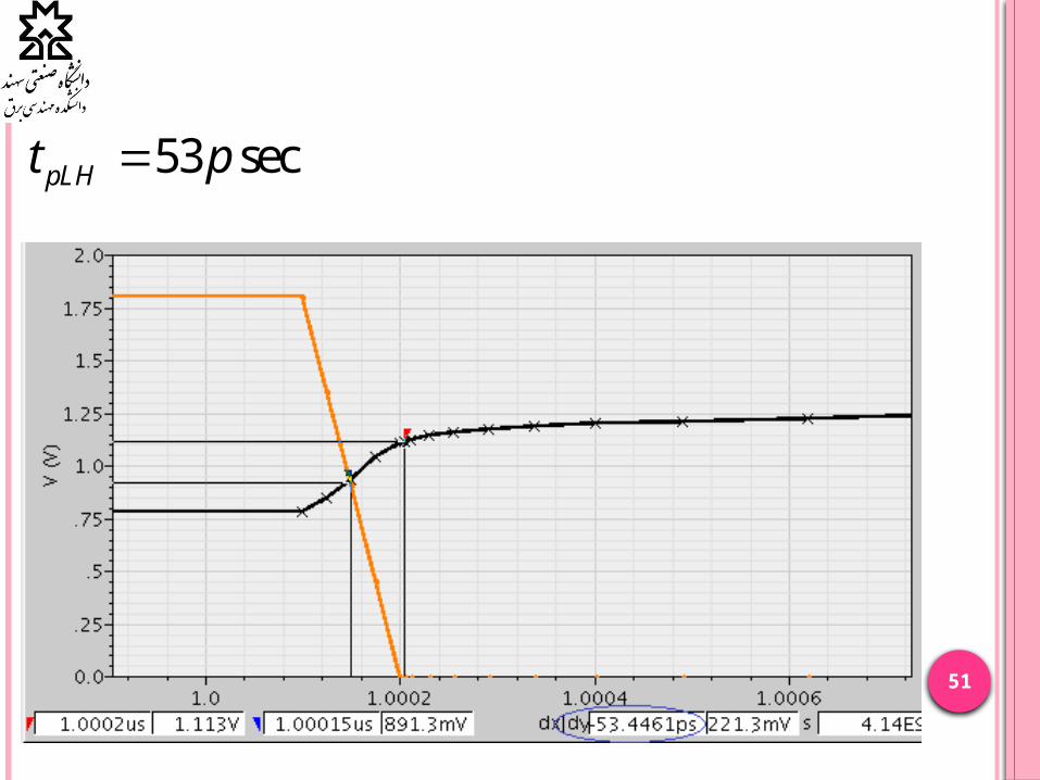
51

53 secpLHt p

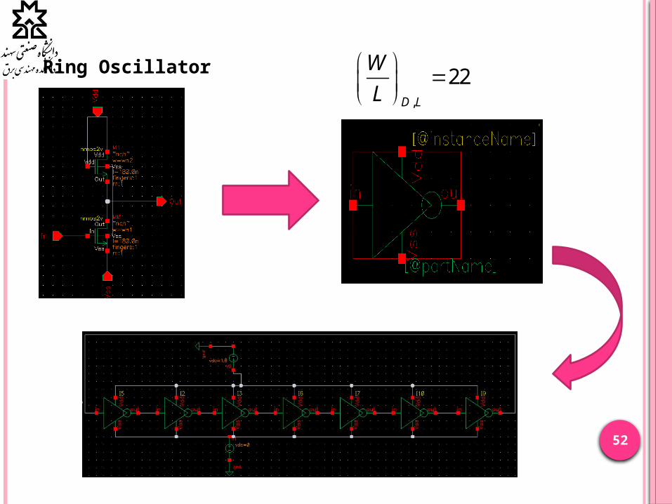
52

Ring Oscillator

,

22D L

W

L

53

Transient simulation

54

1 11.901

526 sec

1 137.5 sec

2 2 7 1.901PP

f f GHzT p

f pn GHz

55

11 1.1OscillationNOT f GHz

21 650OscillatioNOT f MHz

56

Thanks for your attention