Embed Size (px)
Citation preview

1
Data Data AnalysisAnalysis
© 2005 Germaine G Cornelissen-Guillaume. Copying and distribution of this document is permitted in any medium, provided this notice is preserved.

2
Germaine CornélissenGermaine CornélissenUniversity of MinnesotaUniversity of Minnesota
Phoenix presentationPhoenix presentationJuly 10, 2005July 10, 2005
3
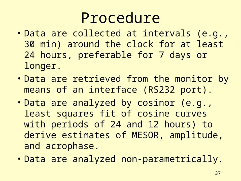
Procedure• Data are collected at intervals (e.g., 30 min) around
the clock for at least 24 hours, preferable for 7 days or longer.
• Data are analyzed by cosinor (e.g., least squares fit of cosine curves with periods of 24 and 12 hours) to derive estimates of MESOR, amplitude, and acrophase.
• Data are analyzed non-parametrically.

4
Ambulatory monitors can be
obtained with a great reduction
in cost with chronobiologic
analyses from the University of
Minnesota ([email protected]),
with results interpreted in the
light of gender- and age-adjusted
archived norms in clinical health.
Opportunity
5
Procedure• Data are collected at intervals (e.g., 30 min) around
the clock for at least 24 hours, preferable for 7 days or longer.
• Data are retrieved from the monitor by means of an interface (RS232 port).
• Data are analyzed non-parametrically.

6
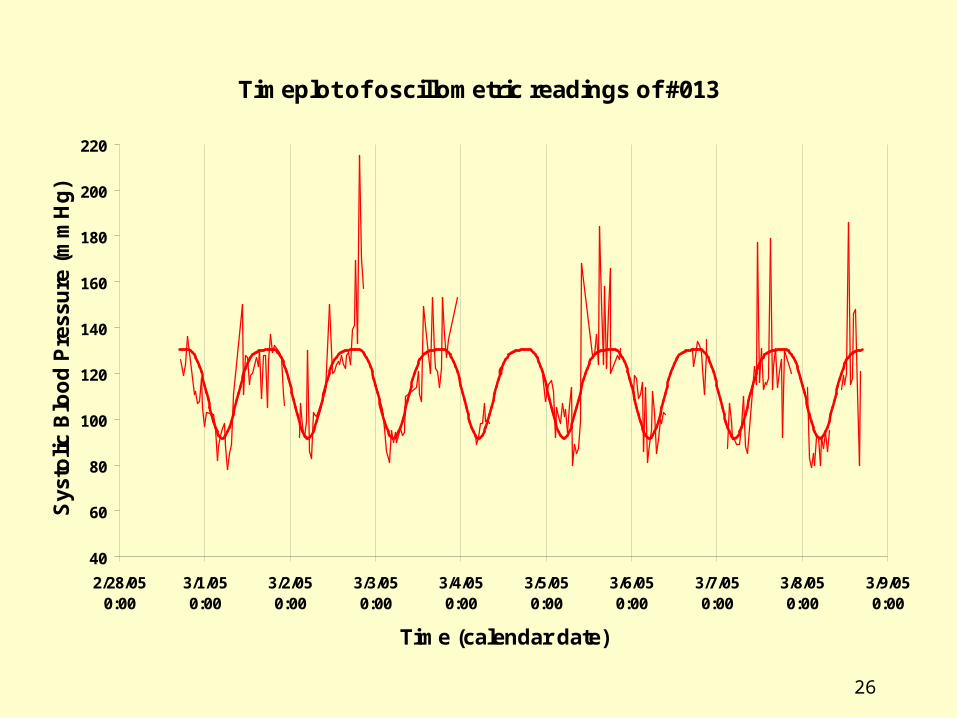
Timeplot of oscillometric readings of #013
40
60
80
100
120
140
160
180
200
220
2/28/050:00
3/1/050:00
3/2/050:00
3/3/050:00
3/4/050:00
3/5/050:00
3/6/050:00
3/7/050:00
3/8/050:00
3/9/050:00
Time (calendar date)
Blo
od
Pre
ssu
re (
mm
Hg
)
0
20
40
60
80
100
120
140
160H
eart Rate (b
eats/min
)
SBP
DBP
HR

7
Procedure• Data are collected at intervals (e.g., 30 min) around
the clock for at least 24 hours, preferable for 7 days or longer.
• Data are retrieved from the monitor by means of an interface (RS232 port).
• Data are analyzed by cosinor (e.g., least squares fit of cosine curves with periods of 24 and 12 hours) to derive estimates of MESOR, amplitude, and acrophase.

8
Let us consider first the case of a single component model.
SINGLE COSINOR METHOD
9
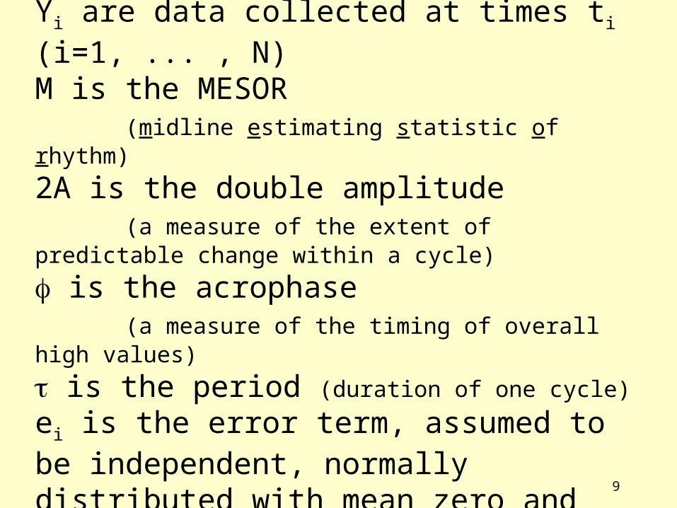
Y(t) = M + Acos(2t/ + ) + e(t)Yi are data collected at times ti (i=1, ... , N)M is the MESOR (midline estimating statistic of rhythm)
2A is the double amplitude (a measure of the extent of predictable change within a cycle)
is the acrophase (a measure of the timing of overall high values)
is the period (duration of one cycle)
ei is the error term, assumed to be independent, normally distributed with mean zero and unknown constant variance 2.
10
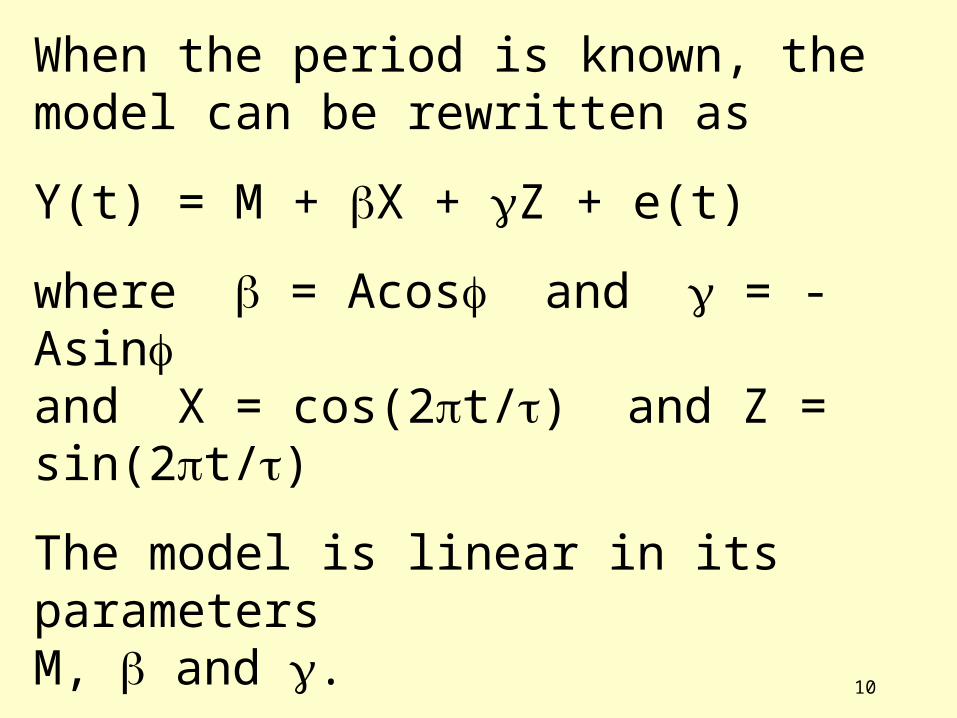
When the period is known, the model can be rewritten as
Y(t) = M + X + Z + e(t)
where = Acos and = -Asinand X = cos(2t/) and Z = sin(2t/)
The model is linear in its parameters M, and .
11
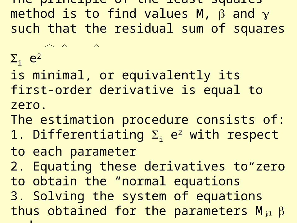
The principle of the least squares method is to find values M, and such that the residual sum of squares
i e2
is minimal, or equivalently its first-order derivative is equal to zero. The estimation procedure consists of:1. Differentiating i e2 with respect to each parameter2. Equating these derivatives to zero to obtain the “normal equations”3. Solving the system of equations thus obtained for the parameters M, and .
12
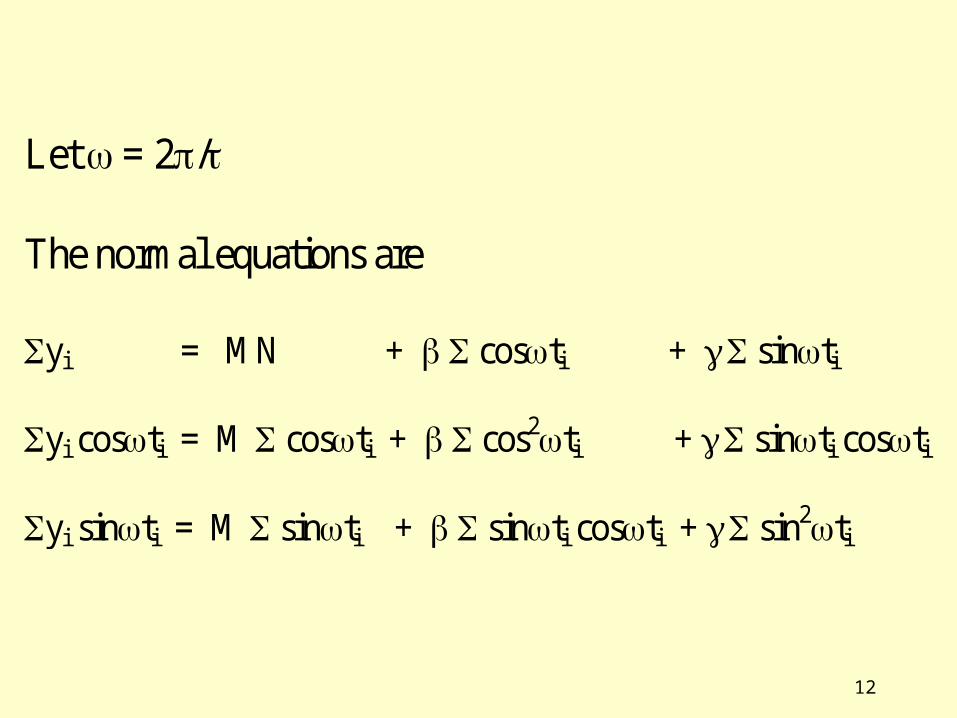
Let = 2/The normal equations are yi = MN + costi + sinti
yi costi = M costi + cos2ti + sinti costi yi sinti = M sinti + sinti costi + sin2ti

13
In matrix form: b = S x or yi N costi sinti M yi costi = costi cos2ti sinti costi yi sinti sinti sinti costi sin2ti

14
The estimates M, , and are obtained by inverting the S matrix x = S-1 b -1
M N costi sinti yi costi cos2ti sinti costi yi costi sinti sinti costi sin2ti yi sinti

15
Estimates for the amplitude and acrophase are then obtained by A = (2 + 2)1/2 = arctan(-/) + K where K is an integer The correct value of is determined by takinf into account the signs of and .
g

16
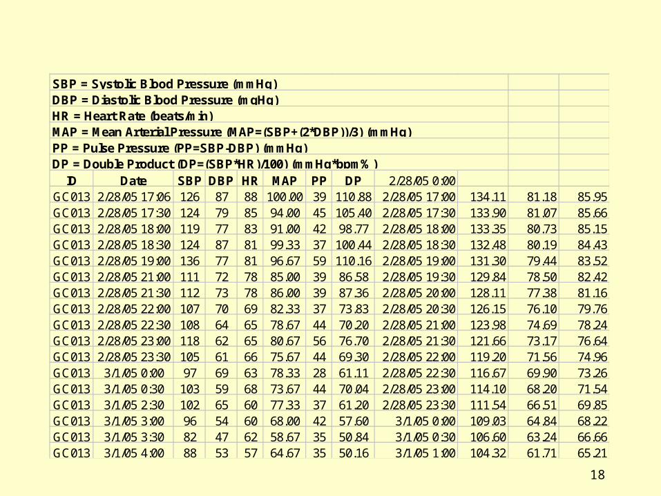
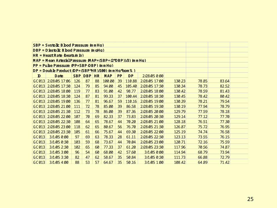
ID Date SBP DBP HR MAP PP DPGC013 2/28/05 17:06 126 87 88 100.00 39 110.88GC013 2/28/05 17:30 124 79 85 94.00 45 105.40GC013 2/28/05 18:00 119 77 83 91.00 42 98.77GC013 2/28/05 18:30 124 87 81 99.33 37 100.44GC013 2/28/05 19:00 136 77 81 96.67 59 110.16GC013 2/28/05 21:00 111 72 78 85.00 39 86.58GC013 2/28/05 21:30 112 73 78 86.00 39 87.36GC013 2/28/05 22:00 107 70 69 82.33 37 73.83GC013 2/28/05 22:30 108 64 65 78.67 44 70.20GC013 2/28/05 23:00 118 62 65 80.67 56 76.70GC013 2/28/05 23:30 105 61 66 75.67 44 69.30GC013 3/1/05 0:00 97 69 63 78.33 28 61.11GC013 3/1/05 0:30 103 59 68 73.67 44 70.04GC013 3/1/05 2:30 102 65 60 77.33 37 61.20GC013 3/1/05 3:00 96 54 60 68.00 42 57.60GC013 3/1/05 3:30 82 47 62 58.67 35 50.84GC013 3/1/05 4:00 88 53 57 64.67 35 50.16
PP = Pulse Pressure (PP=SBP-DBP) (mmHg)DP = Double Product (DP=(SBP*HR)/100) (mmHg*bpm%)
SBP = Systolic Blood Pressure (mmHg)DBP = Diastolic Blood Pressure (mgHg)HR = Heart Rate (beats/min)MAP = Mean Arterial Pressure (MAP=(SBP+(2*DBP))/3) (mmHg)

17
Variable M A SBP 114.447 19.667 -254DBP 68.202 12.975 -255HR 72.913 13.106 -249
Acrophases are expressed in negative degrees, with 360°≡24 hours and 0° set to local midnight.
18
ID Date SBP DBP HR MAP PP DP 2/28/05 0:00GC013 2/28/05 17:06 126 87 88 100.00 39 110.88 2/28/05 17:00 134.11 81.18 85.95GC013 2/28/05 17:30 124 79 85 94.00 45 105.40 2/28/05 17:30 133.90 81.07 85.66GC013 2/28/05 18:00 119 77 83 91.00 42 98.77 2/28/05 18:00 133.35 80.73 85.15GC013 2/28/05 18:30 124 87 81 99.33 37 100.44 2/28/05 18:30 132.48 80.19 84.43GC013 2/28/05 19:00 136 77 81 96.67 59 110.16 2/28/05 19:00 131.30 79.44 83.52GC013 2/28/05 21:00 111 72 78 85.00 39 86.58 2/28/05 19:30 129.84 78.50 82.42GC013 2/28/05 21:30 112 73 78 86.00 39 87.36 2/28/05 20:00 128.11 77.38 81.16GC013 2/28/05 22:00 107 70 69 82.33 37 73.83 2/28/05 20:30 126.15 76.10 79.76GC013 2/28/05 22:30 108 64 65 78.67 44 70.20 2/28/05 21:00 123.98 74.69 78.24GC013 2/28/05 23:00 118 62 65 80.67 56 76.70 2/28/05 21:30 121.66 73.17 76.64GC013 2/28/05 23:30 105 61 66 75.67 44 69.30 2/28/05 22:00 119.20 71.56 74.96GC013 3/1/05 0:00 97 69 63 78.33 28 61.11 2/28/05 22:30 116.67 69.90 73.26GC013 3/1/05 0:30 103 59 68 73.67 44 70.04 2/28/05 23:00 114.10 68.20 71.54GC013 3/1/05 2:30 102 65 60 77.33 37 61.20 2/28/05 23:30 111.54 66.51 69.85GC013 3/1/05 3:00 96 54 60 68.00 42 57.60 3/1/05 0:00 109.03 64.84 68.22GC013 3/1/05 3:30 82 47 62 58.67 35 50.84 3/1/05 0:30 106.60 63.24 66.66GC013 3/1/05 4:00 88 53 57 64.67 35 50.16 3/1/05 1:00 104.32 61.71 65.21
PP = Pulse Pressure (PP=SBP-DBP) (mmHg)DP = Double Product (DP=(SBP*HR)/100) (mmHg*bpm%)
SBP = Systolic Blood Pressure (mmHg)DBP = Diastolic Blood Pressure (mgHg)HR = Heart Rate (beats/min)MAP = Mean Arterial Pressure (MAP=(SBP+(2*DBP))/3) (mmHg)
19
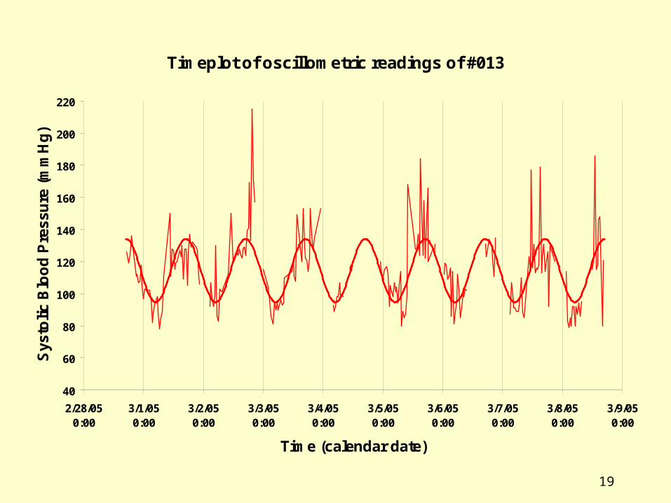
Timeplot of oscillometric readings of #013
40
60
80
100
120
140
160
180
200
220
2/28/050:00
3/1/050:00
3/2/050:00
3/3/050:00
3/4/050:00
3/5/050:00
3/6/050:00
3/7/050:00
3/8/050:00
3/9/050:00
Time (calendar date)
Sys
toli
c B
loo
d P
ress
ure
(m
mH
g)

20
Timeplot of oscillometric readings of #013
30
50
70
90
110
130
150
2/28/050:00
3/1/050:00
3/2/050:00
3/3/050:00
3/4/050:00
3/5/050:00
3/6/050:00
3/7/050:00
3/8/050:00
3/9/050:00
Time (calendar date)
Dia
sto
lic
Blo
od
Pre
ssu
re (
mm
Hg
)

21
Timeplot of oscillometric readings of #013
30
50
70
90
110
130
150
2/28/050:00
3/1/050:00
3/2/050:00
3/3/050:00
3/4/050:00
3/5/050:00
3/6/050:00
3/7/050:00
3/8/050:00
3/9/050:00
Time (calendar date)
Hea
rt R
ate
(bea
ts/m
in)

22
The model is easily extended to include more than a single component: Y(t) = M + i Aicos(2t/i + i) + e(t) i=1, ..., k A system of 2k+1 normal equations with 2k+1 parameters needs to be resolved in this case. The parameters are M and (Ai, i) of cosine curves with periods i, i=1, …, k. Usually, a 2-component model is considered with periods of 24 and 12 hours.
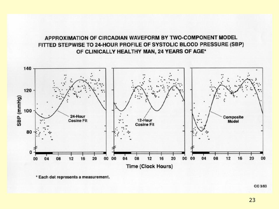
23
24
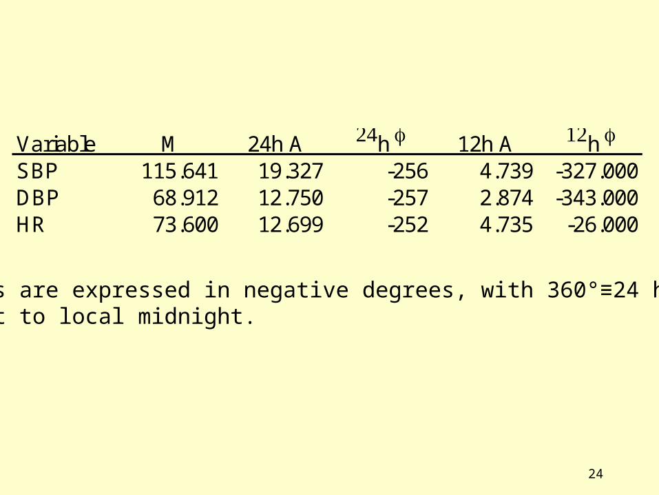
Variable M 24h A h 12h A hSBP 115.641 19.327 -256 4.739 -327.000DBP 68.912 12.750 -257 2.874 -343.000HR 73.600 12.699 -252 4.735 -26.000
Acrophases are expressed in negative degrees, with 360°≡24 hours and 0° set to local midnight.
25
ID Date SBP DBP HR MAP PP DP 2/28/05 0:00GC013 2/28/05 17:06 126 87 88 100.00 39 110.88 2/28/05 17:00 130.23 78.85 83.64GC013 2/28/05 17:30 124 79 85 94.00 45 105.40 2/28/05 17:30 130.34 78.73 82.52GC013 2/28/05 18:00 119 77 83 91.00 42 98.77 2/28/05 18:00 130.42 78.59 81.43GC013 2/28/05 18:30 124 87 81 99.33 37 100.44 2/28/05 18:30 130.45 78.42 80.42GC013 2/28/05 19:00 136 77 81 96.67 59 110.16 2/28/05 19:00 130.39 78.21 79.54GC013 2/28/05 21:00 111 72 78 85.00 39 86.58 2/28/05 19:30 130.19 77.94 78.79GC013 2/28/05 21:30 112 73 78 86.00 39 87.36 2/28/05 20:00 129.79 77.59 78.18GC013 2/28/05 22:00 107 70 69 82.33 37 73.83 2/28/05 20:30 129.14 77.12 77.70GC013 2/28/05 22:30 108 64 65 78.67 44 70.20 2/28/05 21:00 128.18 76.51 77.30GC013 2/28/05 23:00 118 62 65 80.67 56 76.70 2/28/05 21:30 126.87 75.72 76.95GC013 2/28/05 23:30 105 61 66 75.67 44 69.30 2/28/05 22:00 125.19 74.74 76.58GC013 3/1/05 0:00 97 69 63 78.33 28 61.11 2/28/05 22:30 123.13 73.55 76.15GC013 3/1/05 0:30 103 59 68 73.67 44 70.04 2/28/05 23:00 120.71 72.16 75.59GC013 3/1/05 2:30 102 65 60 77.33 37 61.20 2/28/05 23:30 117.96 70.56 74.87GC013 3/1/05 3:00 96 54 60 68.00 42 57.60 3/1/05 0:00 114.94 68.79 73.94GC013 3/1/05 3:30 82 47 62 58.67 35 50.84 3/1/05 0:30 111.73 66.88 72.79GC013 3/1/05 4:00 88 53 57 64.67 35 50.16 3/1/05 1:00 108.42 64.89 71.42
PP = Pulse Pressure (PP=SBP-DBP) (mmHg)DP = Double Product (DP=(SBP*HR)/100) (mmHg*bpm%)
SBP = Systolic Blood Pressure (mmHg)DBP = Diastolic Blood Pressure (mgHg)HR = Heart Rate (beats/min)MAP = Mean Arterial Pressure (MAP=(SBP+(2*DBP))/3) (mmHg)
26
Timeplot of oscillometric readings of #013
40
60
80
100
120
140
160
180
200
220
2/28/050:00
3/1/050:00
3/2/050:00
3/3/050:00
3/4/050:00
3/5/050:00
3/6/050:00
3/7/050:00
3/8/050:00
3/9/050:00
Time (calendar date)
Sys
toli
c B
loo
d P
ress
ure
(m
mH
g)
27
Timeplot of oscillometric readings of #013
30
50
70
90
110
130
150
2/28/050:00
3/1/050:00
3/2/050:00
3/3/050:00
3/4/050:00
3/5/050:00
3/6/050:00
3/7/050:00
3/8/050:00
3/9/050:00
Time (calendar date)
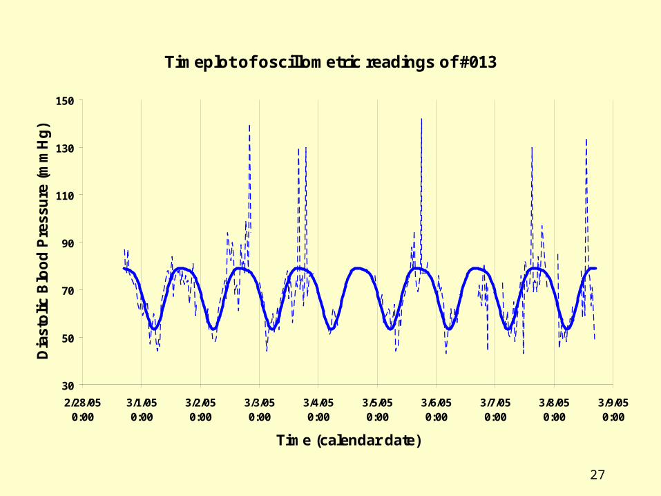
Dia
sto
lic
Blo
od
Pre
ssu
re (
mm
Hg
)
28
Timeplot of oscillometric readings of #013
30
50
70
90
110
130
150
2/28/050:00
3/1/050:00
3/2/050:00
3/3/050:00
3/4/050:00
3/5/050:00
3/6/050:00
3/7/050:00
3/8/050:00
3/9/050:00
Time (calendar date)
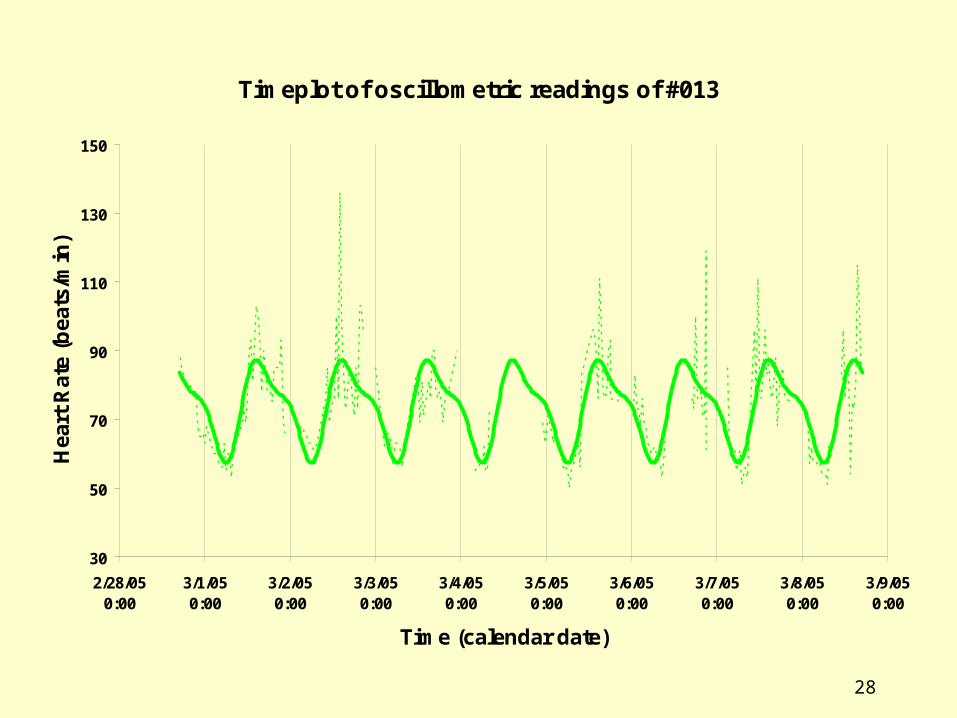
Hea
rt R
ate
(bea
ts/m
in)
29
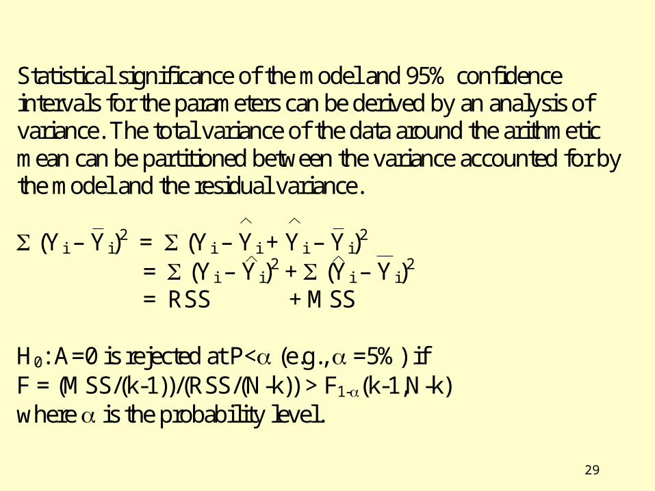
Statistical significance of the model and 95% confidence intervals for the parameters can be derived by an analysis of variance. The total variance of the data around the arithmetic mean can be partitioned between the variance accounted for by the model and the residual variance. (Yi – Yi)
2 = (Yi – Yi + Yi – Yi)2
= (Yi – Yi)2 + (Yi – Yi)
2 = RSS + MSS H0: A=0 is rejected at P< (e.g., =5%) if F = (MSS/(k-1))/(RSS/(N-k)) > F1-(k-1,N-k) where is the probability level.

30
Acrophase Hour Variable PR P MESOR S.E. Amplitude S.E. ( 95.0 %CI ) phi SE (95.0 %CI) ------------------------------------------------------------------------------------------------------------------------------------------ 1 SBP 49 < .001 114.447 1.026 19.667 1.402 ( 17.12, 22.21) -254 5 (-245,-264) 1658 2 DBP 41 < .001 68.202 0.804 12.975 1.094 ( 10.98, 14.97) -255 5 (-244,-267) 1702 3 HR 53 < .001 72.913 0.636 13.106 0.888 ( 11.52, 14.69) -249 4 (-241,-258) 1638 ------------------------------------------------------------------------------------------------------------------------------------------ Acrophase
Variable Period MESOR ± S.E. PR P Amplitude S.E. ( 95.0 %CI ) phi SE (95.0 %CI) --------------------------------------------------------------------------------------------------------------------------------------- 1 SBP 115.641 1.081 24.00 48 < .001 19.327 1.369 ( 16.64, 22.01) -256 5 (-247,-266) 12.00 3 0.009 4.739 1.428 ( 1.94, 7.54) -327 19 (-291, -4) overall 51 < .001 --------------------------------------------------------------------------------------------------------------------------------------- 2 DBP 68.912 0.854 24.00 40 < .001 12.750 1.077 ( 10.64, 14.86) -257 6 (-246,-268) 12.00 2 0.057 2.874 1.144 ( 0.63, 5.12) -343 24 (-296, -30) overall 42 < .001 --------------------------------------------------------------------------------------------------------------------------------------- 3 HR 73.600 0.643 24.00 51 < .001 12.699 0.829 ( 11.07, 14.32) -252 4 (-244,-260) 12.00 7 < .001 4.735 0.907 ( 2.96, 6.51) -26 10 ( -6, -46) overall 58 < .001 --------------------------------------------------------------------------------------------------------------------------------------- PR = MSS/(MSS+RSS) = R2.

31
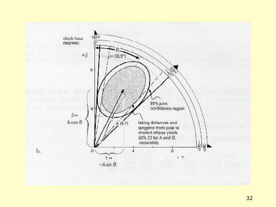
When F is evaluated at A = A instead of at A=0, the equation obtained is that of an ellipse representing the confidence region for (, ) or equivalently for (A, ). Conservative confidence intervals for A and can be derived by computing the minimal and maximal distances from the pole to the error ellipse and by drawing the tangents from the pole to the error ellipse, respectively.
32
33
Results from the parametric approach are reported in the sphygmochron
where they are compared with 90% prediction limits from healthy peers
matched by gender and age.

34
Name:--------------------- Patient #: GCor013Age: 55 Sex: F
To:
Patient Peer Group Patient Peer Group Patient Peer GroupValue Reference Value Reference Value Reference
Limits Limits Limits
Range Range Range
Range Range Range
Range Range Range
Individualized bounded indices: (STD = Standard)(Min = Minimum)(Max = Maximum)(HBI = Hyperbanic Index)
No AnnuallyYes Drug Non-Drug As soon as possible
Other specify_________________________
Prepared By_________________________________________ Date____/____/________
1) Unusually long standing or lying down during waking: unusual activity, such as exercise, emotional
loads, or schedule changes, e.g. shiftwork; etc.; 2) Salt, calories, kind and amount, other, etc.
Copyright, Halberg Chronobiology Center, University of Minnesota, Mayo Hospital, Rooms 715,
733-5 (7th floor), Minneapolis Campus, Del Code 8609, 420 Deleware Street SE,
Minneapolis, MN 55455, USA. Fax 612-624-9989.
For questions, call F. Halberg or G. Cornelissen at 612-624-6976.
3/8/2005 16:30
STD (MIN; MAX)* STD (MIN; MAX)* STD (MIN; MAX)*
25.40 3.07-28.70
17:05 10:46-18:46 17:09 10:45-17:26 16:48 8:52-19:09
HEART RATE (bpm)
115.6 102.2-138.6 68.9 67.4-86.5 73.6 65.3-86.3
HIGH VALUES(ACROPHASE) (hr:min)
SYSTOLIC BP (mmHg) DIASTOLIC BP (mmHg)
38.65 3.27-37.15 25.50 4.01-26.50
(MESOR)
PREDICTABLE CHANGE(DOUBLE AMPLITUDE)
TIMING OF OVERALL
Monitoring From:Comments:
CHRONOBIOLOGIC CHARACTERISTICS
ADJUSTED 24-h MEAN
2/28/2005 17:06
SPHYGMOCHRON-TM Monitoring Profile over Time;Computer Comparison with Peer Group Limits
Blood Pressure (BP) and Related Cardiovascular Summary.
The double amplitude of systolic blood pressure is above the upper 95% prediction limit: systolic CHAT is diagnosed.
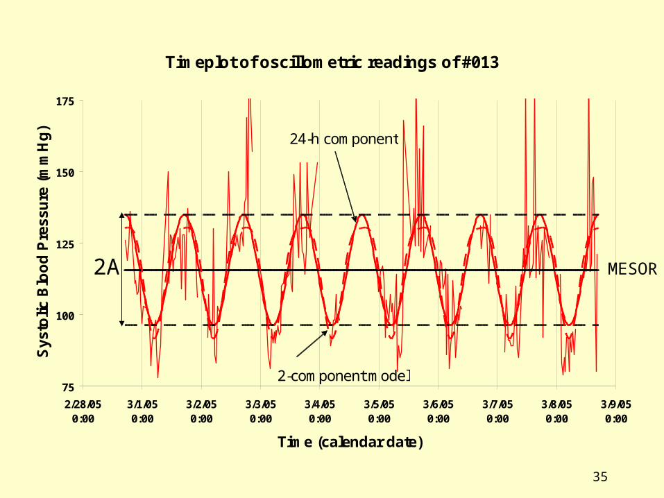
35
Timeplot of oscillometric readings of #013
75
100
125
150
175
2/28/050:00
3/1/050:00
3/2/050:00
3/3/050:00
3/4/050:00
3/5/050:00
3/6/050:00
3/7/050:00
3/8/050:00
3/9/050:00
Time (calendar date)
Sys
toli
c B
loo
d P
ress
ure
(m
mH
g)
24-h component
2-component model
MESOR2A

36
37
Procedure• Data are collected at intervals (e.g., 30 min) around
the clock for at least 24 hours, preferable for 7 days or longer.
• Data are retrieved from the monitor by means of an interface (RS232 port).
• Data are analyzed by cosinor (e.g., least squares fit of cosine curves with periods of 24 and 12 hours) to derive estimates of MESOR, amplitude, and acrophase.
• Data are analyzed non-parametrically.

38
39
40
41
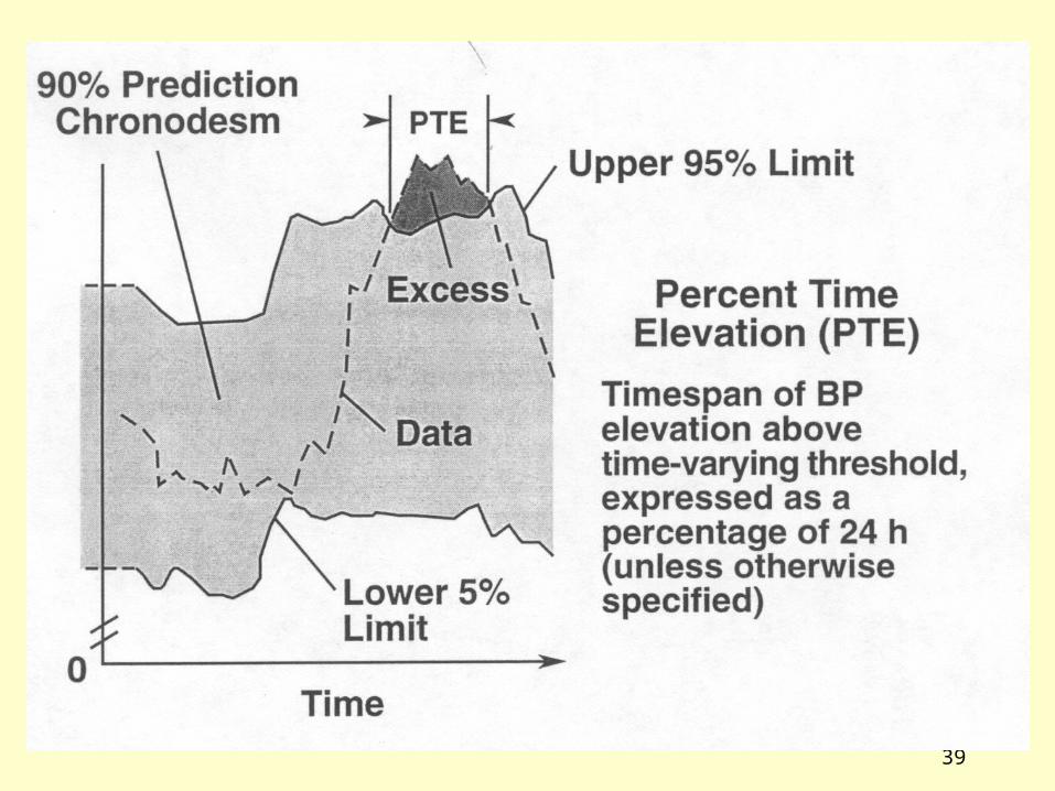
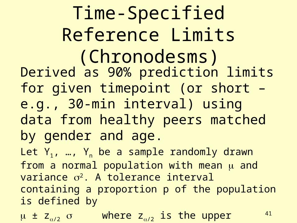
Time-Specified Reference Limits(Chronodesms)
Derived as 90% prediction limits for given timepoint (or short – e.g., 30-min interval) using data from healthy peers matched by gender and age.Let Y1, …, Yn be a sample randomly drawn from a normal population with mean and variance 2. A tolerance interval containing a proportion p of the population is defined by ± z/2 where z/2 is the upper (1-/2) fractile of the standard normal curve (e.g., 1.96 for = 0.05). This interval covers a fraction (1-) of the population.
42
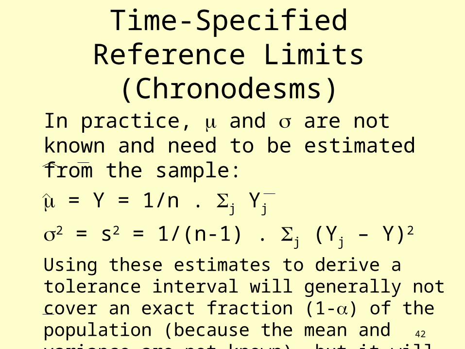
Time-Specified Reference Limits(Chronodesms)
In practice, and are not known and need to be estimated from the sample:
= Y = 1/n . j Yj
2 = s2 = 1/(n-1) . j (Yj – Y)2
Using these estimates to derive a tolerance interval will generally not cover an exact fraction (1-) of the population (because the mean and variance are not known), but it will do so on the average.
Y ± t/2; (n-1) s [(n+1)/n]1/2 (t = Student distribution).
43
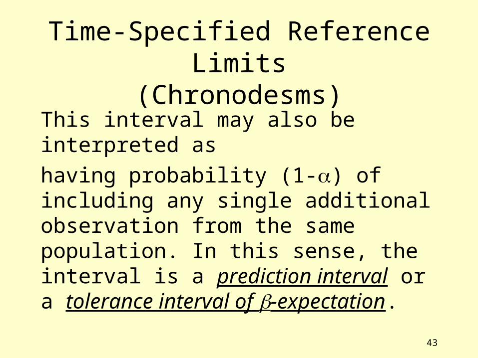
Time-Specified Reference Limits(Chronodesms)
This interval may also be interpreted as
having probability (1-) of including any single additional observation from the same population. In this sense, the interval is a prediction interval or a tolerance interval of -expectation.
44
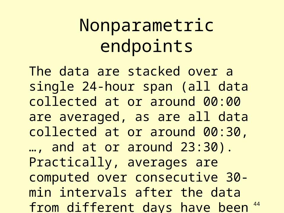
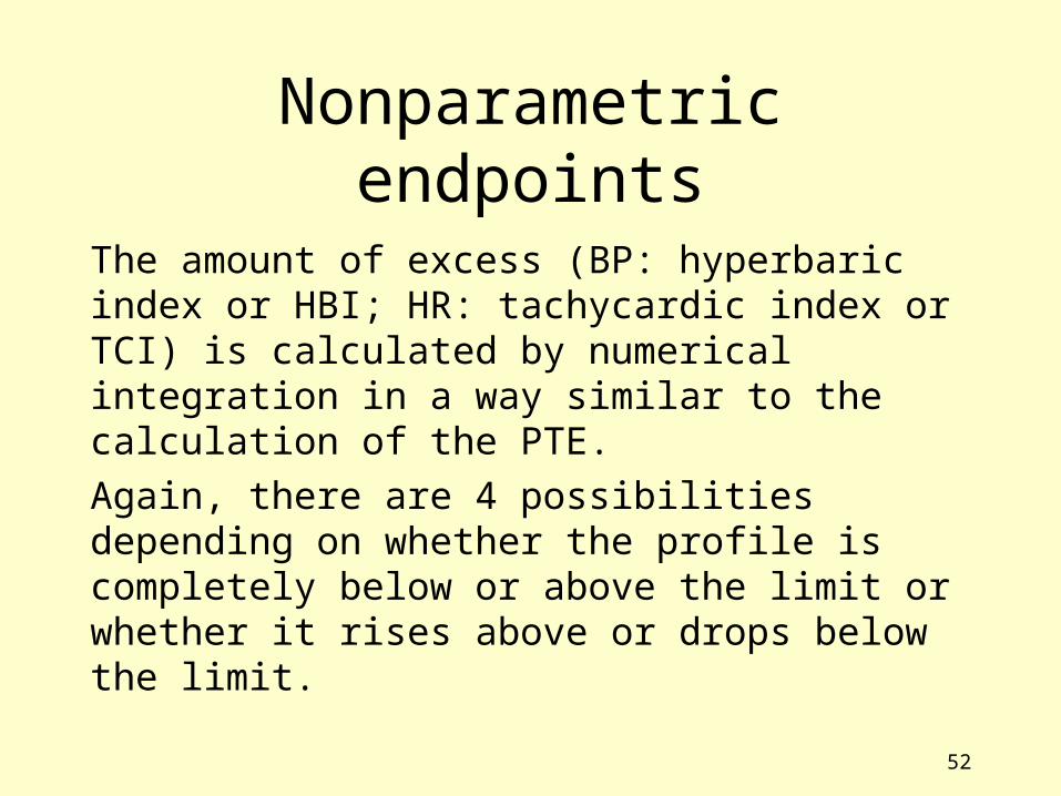
Nonparametric endpoints
The data are stacked over a single 24-hour span (all data collected at or around 00:00 are averaged, as are all data collected at or around 00:30, …, and at or around 23:30). Practically, averages are computed over consecutive 30-min intervals after the data from different days have been stacked.

45
Circadian Pattern of SBP (#013, F, 55y)
80
90
100
110
120
130
140
150
160
0:00 2:00 4:00 6:00 8:00 10:00 12:00 14:00 16:00 18:00 20:00 22:00 0:00
Time (Clock Hours)
SB
P (
mm
Hg
)

46
Nonparametric endpoints
A scan from 00:00 to 24:00 is conducted to determine whether the profile at that time is within the prediction interval or whether it is above the upper 95% prediction limit. If so, using linear interpolation, the amount of time the profile was excessive is estimated and summed over the 24-hour span. The total is divided by 24 hours to yield the percentage time elevation (PTE).
47
For each (e.g., 30-min) interval,there are 4 different possibilities.

48
114
115
116
117
118
119
120
121
122
123
0:30 1:00 1:30 2:00
Time (clock hours)
SB
P (
mm
Hg
)Reference Profile
Partial PTE = 0
49
114
116
118
120
122
124
126
1:00 1:30 2:00 2:30
Time (clock hours)
SB
P (
mm
Hg
)Reference Profile
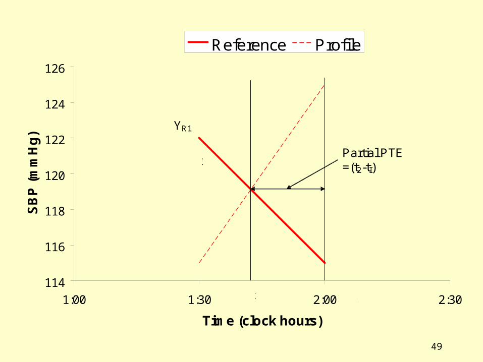
Partial PTE=(t2-tI)
YR1
YR2Yp1
Yp2
Y1(t) = YR1 + (YR2-YR1)tY2(t) = Yp1 + (Yp2-Yp1)t
Y1(t) = Y2(t)
tI = (YR1-Yp1)/(Yp-YR)
where Y is Y(t2)-Y(t1)
tI (t2)
50
110
112
114
116
118
120
122
124
126
1:30 2:00 2:30 3:00
Time (clock hours)
SB
P (
mm
Hg
)Reference Profile
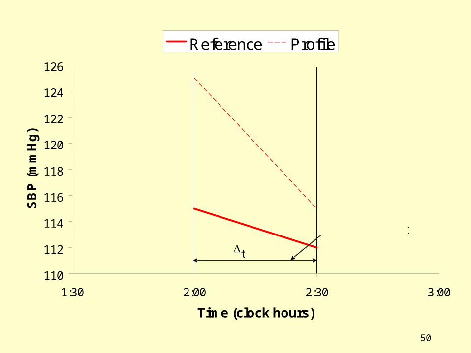
Partial PTE = t
t
51
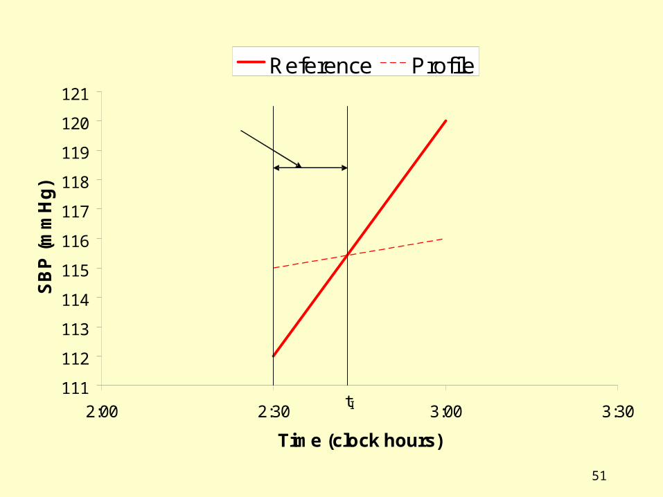
111
112
113
114
115
116
117
118
119
120
121
2:00 2:30 3:00 3:30
Time (clock hours)
SB
P (
mm
Hg
)Reference Profile
Partial PTE = (tI - t1)
tI(t1)
52
Nonparametric endpoints
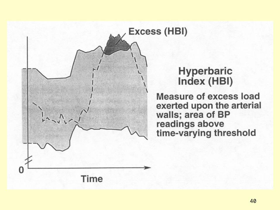
The amount of excess (BP: hyperbaric index or HBI; HR: tachycardic index or TCI) is calculated by numerical integration in a way similar to the calculation of the PTE.
Again, there are 4 possibilities depending on whether the profile is completely below or above the limit or whether it rises above or drops below the limit.

53
114
115
116
117
118
119
120
121
122
123
0:30 1:00 1:30 2:00
Time (clock hours)
SB
P (
mm
Hg
)Reference Profile
Partial HBI = 0
54
114
116
118
120
122
124
126
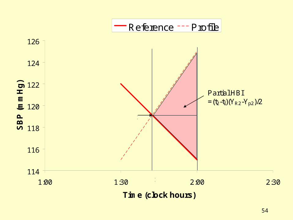
1:00 1:30 2:00 2:30
Time (clock hours)
SB
P (
mm
Hg
)Reference Profile
Partial HBI=(t2-tI)(YR2-Yp2)/2
YR1
YR2Yp1
Yp2
tI = (YR1-Yp1)/(Yp-YR)
where Y is Y(t2)-Y(t1)
YI =Y(tI) = YR1 + (YR2-YR1)tI = Yp1 + (Yp2-Yp1)tI
tI (t2)
YI
55
110
112
114
116
118
120
122
124
126
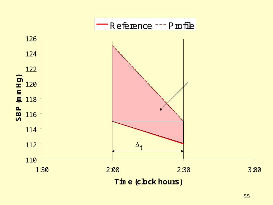
1:30 2:00 2:30 3:00
Time (clock hours)
SB
P (
mm
Hg
)Reference Profile
Partial HBI = t (Yp2-YR1) +t (YR2-YR1+ Yp1-Yp2)/2
t
56
111
112
113
114
115
116
117
118
119
120
121
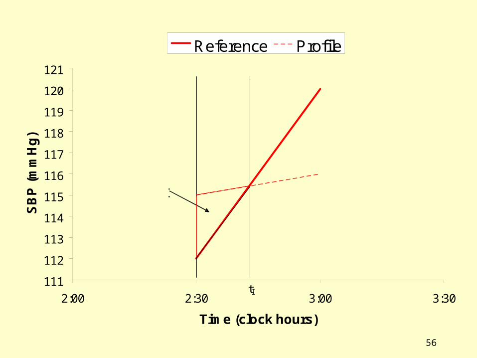
2:00 2:30 3:00 3:30
Time (clock hours)
SB
P (
mm
Hg
)Reference Profile
Partial HBI
tI(t1)
57
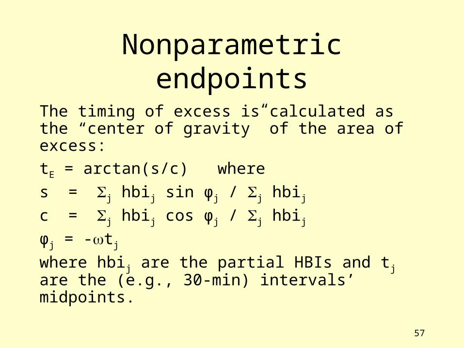
Nonparametric endpoints
The timing of excess is calculated as the “center of gravity” of the area of excess:
tE = arctan(s/c) where
s = j hbij sin φj / j hbij
c = j hbij cos φj / j hbij
φj = -tj
where hbij are the partial HBIs and tj are the (e.g., 30-min) intervals’ midpoints.
58
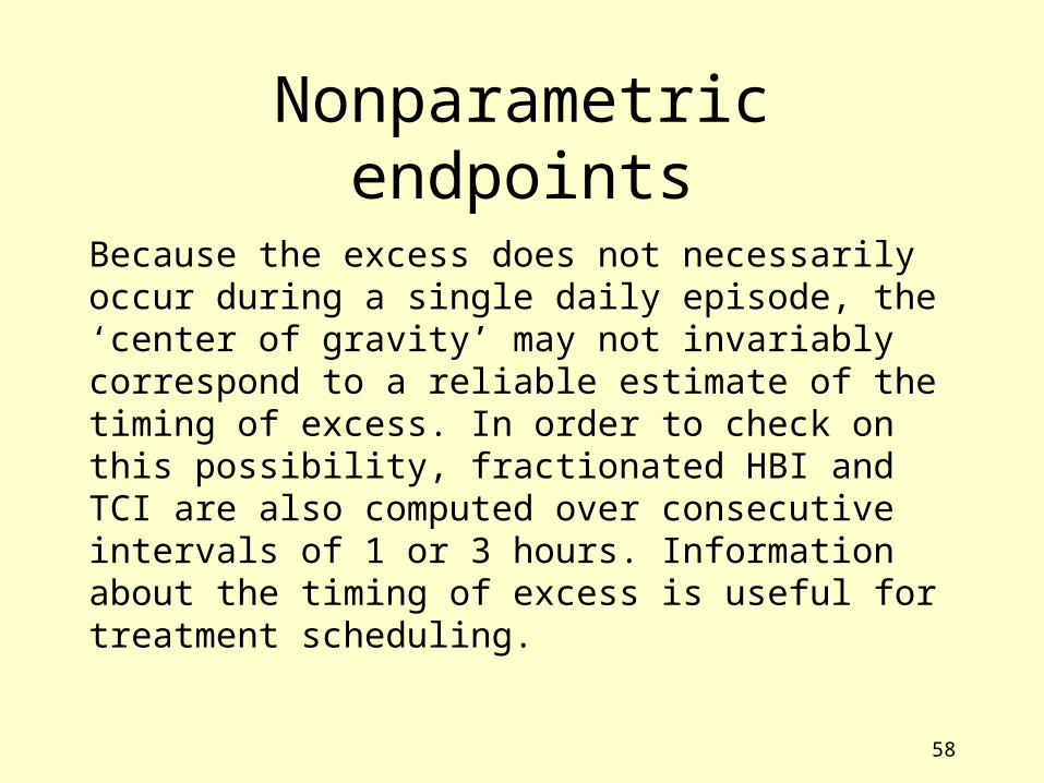
Nonparametric endpoints
Because the excess does not necessarily occur during a single daily episode, the ‘center of gravity’ may not invariably correspond to a reliable estimate of the timing of excess. In order to check on this possibility, fractionated HBI and TCI are also computed over consecutive intervals of 1 or 3 hours. Information about the timing of excess is useful for treatment scheduling.

59
Circadian Pattern of SBP (GCor013, F, 55y)
80
90
100
110
120
130
140
150
160
0:00 2:00 4:00 6:00 8:00 10:00 12:00 14:00 16:00 18:00 20:00 22:00 0:00
Time (Clock Hours)
SB
P (
mm
Hg
)
SBP
SBP-lo
SBP-hi
60
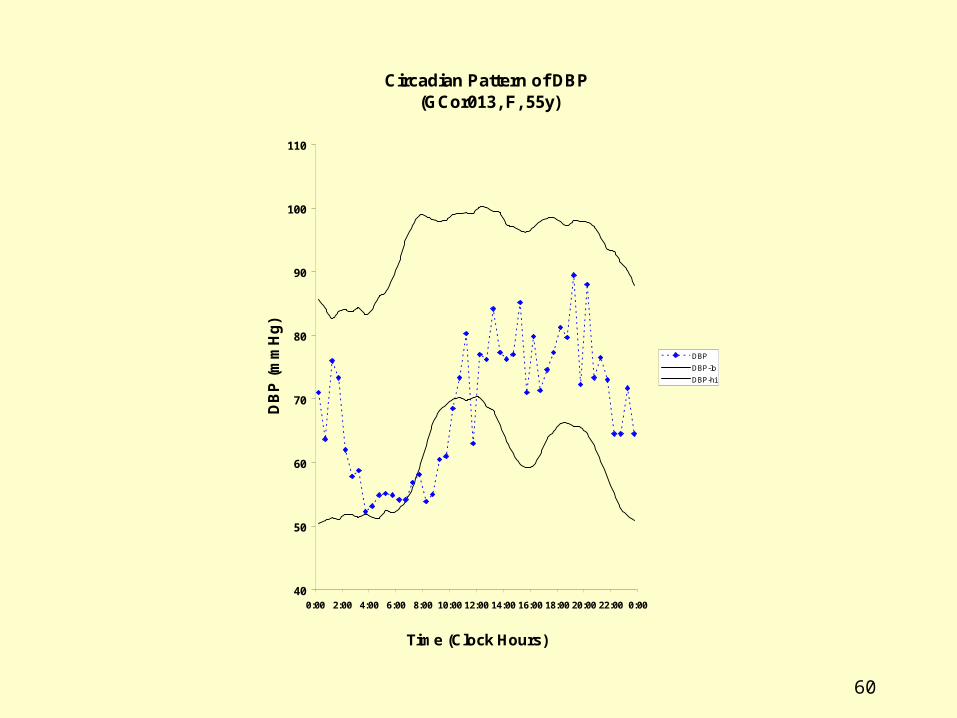
Circadian Pattern of DBP (GCor013, F, 55y)
40
50
60
70
80
90
100
110
0:00 2:00 4:00 6:00 8:00 10:00 12:00 14:00 16:00 18:00 20:00 22:00 0:00
Time (Clock Hours)
DB
P (
mm
Hg
)
DBP
DBP-lo
DBP-hi
61
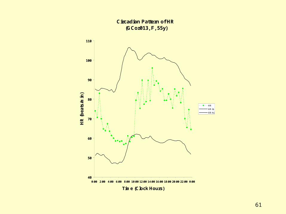
Circadian Pattern of HR (GCor013, F, 55y)
40
50
60
70
80
90
100
110
0:00 2:00 4:00 6:00 8:00 10:00 12:00 14:00 16:00 18:00 20:00 22:00 0:00
Time (Clock Hours)
HR
(b
eats
/min
)
HR
HR-lo
HR-hi
62
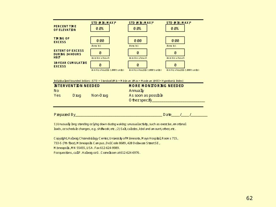
Name:--------------------- Patient #: GCor013Age: 55 Sex: F
To:
(hr:min) (hr:min) (hr:min)
(mmHg x hour) (mmHg x hour) (mmHg x hour)
(mmHg x hour)(in 1,000's units) (mmHg x hour)(in 1,000's units) (mmHg x hour)(in 1,000's units)
Individualized bounded indices: (STD = Standard)(Min = Minimum)(Max = Maximum)(HBI = Hyperbanic Index)
INTERVENTION NEEDED MORE MONITORING NEEDEDNo AnnuallyYes Drug Non-Drug As soon as possible
Other specify_________________________
Prepared By_________________________________________ Date____/____/________
1) Unusually long standing or lying down during waking: unusual activity, such as exercise, emotional
loads, or schedule changes, e.g. shiftwork; etc.; 2) Salt, calories, kind and amount, other, etc.
Copyright, Halberg Chronobiology Center, University of Minnesota, Mayo Hospital, Rooms 715,
733-5 (7th floor), Minneapolis Campus, Del Code 8609, 420 Deleware Street SE,
Minneapolis, MN 55455, USA. Fax 612-624-9989.
For questions, call F. Halberg or G. Cornelissen at 612-624-6976.
0 0 0
STD (MIN; MAX)* STD (MIN; MAX)* STD (MIN; MAX)*
0.0% 0.0% 0.0%
0 0 0EXCESS
0:00 0:00 0:00
EXTENT OF EXCESSDURING 24 HOURSHBI*
10-YEAR CUMULATIVE
PERCENT TIMEOF ELEVATION
TIMING OFEXCESS

63
Comments• Reference values are now computed in terms of clock hours.
It would be preferable to compute them in relation to the usual rest-activity schedule of each individual. Hence the merit of a diary.
• Reference values are now computed for a finite number of groups specified by gender and age with a special set of reference values for pregnant women. It would be preferable to determine overall trends with age for women, men and pregnant women in terms of the MESOR and circadian amplitude and acrophase to have a continuum of values.
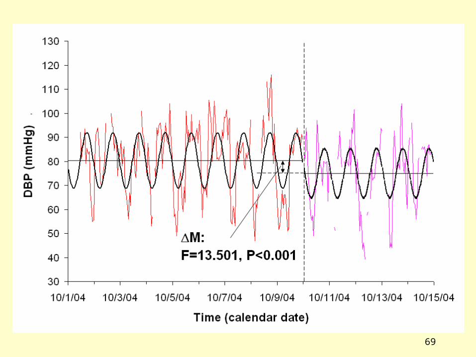
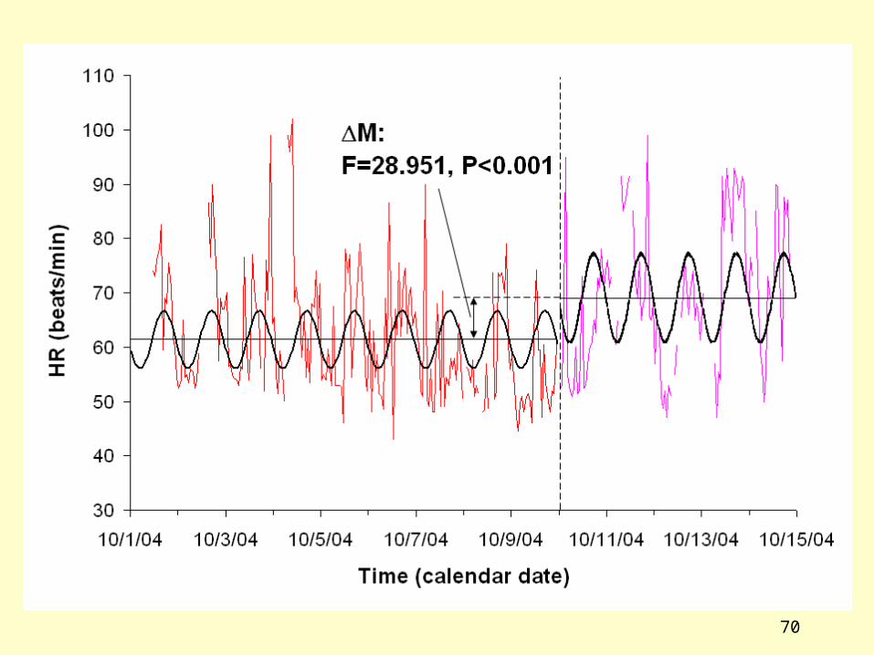
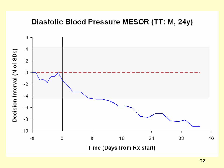
• When repeated profiles are obtained for the same person, additional methods are available such as parameter tests and cumulative sums (CUSUMs) that can assess any changes in rhythm characteristics as a function of time (e.g., in relation to a given intervention such as medication).

64
65
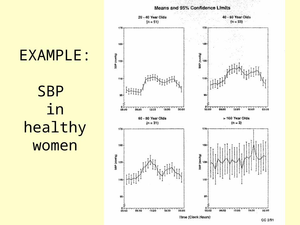
EXAMPLE:
SBP in healthy women

66
Comments• Reference values are now computed in terms of clock hours.
It would be preferable to compute them in relation to the usual rest-activity schedule of each individual. Hence the merit of a diary.
• Reference values are now computed for a finite number of groups specified by gender and age with a special set of reference values for pregnant women. It would be preferable to determine overall trends with age for women, men and pregnant women in terms of the MESOR and circadian amplitude and acrophase to have a continuum of values.
• When repeated profiles are obtained for the same person, additional methods are available such as parameter tests and cumulative sums (CUSUMs) that can assess any changes in rhythm characteristics as a function of time (e.g., in relation to a given intervention such as medication).

67

68
69
70

71
72


![Lippincott Illustrated Reviews Flash Cards Microbiology - Cornelissen [SRG]](https://img.dokumen.tips/doc/110x75/55cf8ee7550346703b96d934/lippincott-illustrated-reviews-flash-cards-microbiology-cornelissen-srg.jpg)