1

CSE 881: Data Mining

Lecture 6: Model Overfitting and Classifier Evaluation

Read Sections 4.4 – 4.6

2

Classification Errors

Training errors (apparent errors)

– Errors committed on the training set

Test errors

– Errors committed on the test set

Generalization errors

– Expected error of a model over random selection of records from same distribution

3

Example Data Set

Two class problem:

+, o

3000 data points (30% for training, 70% for testing)

Data set for + class is generated from a uniform distribution

Data set for o class is generated from a mixture of 3 gaussian distributions, centered at (5,15), (10,5), and (15,15)

4

Decision Trees

x1 < 13.29 x2 < 17.35

x2 < 12.63

x1 < 6.56

x2 < 8.64

x2 < 1.38

x1 < 2.15

x1 < 7.24

x1 < 12.11

x1 < 18.88

x1 < 13.29

x2 < 17.35

x1 < 6.56

x2 < 8.64

x2 < 1.38

x1 < 2.15

x1 < 7.24

x1 < 12.11

x1 < 18.88x2 < 4.06

x1 < 6.99

x1 < 6.78

x2 < 19.93

x1 < 3.03

x2 < 12.68x1 < 2.72

x2 < 15.77 x2 < 17.14

x2 < 12.89

x2 < 13.80

x2 < 16.75

x2 < 16.33

Decision Tree with 11 leaf nodes Decision Tree with 24 leaf nodes

Which tree is better?

5

Model Overfitting

Underfitting: when model is too simple, both training and test errors are large

Overfitting: when model is too complex, training error is small but test error is large

6

Mammal Classification Problem

BodyTemperature

Give Birth

Warm Cold

Yes No

MammalsNon-

mammals

Non-mammals

Training Set

Decision Tree Model

training error = 0%

7

Effect of Noise

Training Set:

Test Set:

Example: Mammal Classification problem

BodyTemperature

Give Birth

Warm-blooded Cold-blooded

Yes No

MammalsNon-

mammals

Non-mammals

Model M1:

train err = 0%,

test err = 30%

Model M2:

train err = 20%,

test err = 10%

Give Birth

Four-legged

Yes No

Yes No

MammalsNon-

mammals

Non-mammals

BodyTemperature

Warm-blooded Cold-blooded

Non-mammals

8

Lack of Representative Samples

BodyTemperature

Hibernates

Warm-blooded Cold-blooded

Yes No

Non-mammals

Non-mammals

Mammals

Four-legged

Yes No

Non-mammals

Lack of training records at the leaf nodes for making reliable classification

Training Set:

Test Set:

Model M3:

train err = 0%,

test err = 30%

9

Effect of Multiple Comparison Procedure

Consider the task of predicting whether stock market will rise/fall in the next 10 trading days

Random guessing:

P(correct) = 0.5

Make 10 random guesses in a row:

Day 1 Up

Day 2 Down

Day 3 Down

Day 4 Up

Day 5 Down

Day 6 Down

Day 7 Up

Day 8 Up

Day 9 Up

Day 10 Down

0547.02

10

10

9

10

8

10

)8(#10

correctP

10

Effect of Multiple Comparison Procedure

Approach:

– Get 50 analysts

– Each analyst makes 10 random guesses

– Choose the analyst that makes the most number of correct predictions

Probability that at least one analyst makes at least 8 correct predictions

9399.0)0547.01(1)8(# 50 correctP

11

Effect of Multiple Comparison Procedure

Many algorithms employ the following greedy strategy:– Initial model: M– Alternative model: M’ = M ,

where is a component to be added to the model (e.g., a test condition of a decision tree)

– Keep M’ if improvement, (M,M’) >

Often times, is chosen from a set of alternative components, = {1, 2, …, k}

If many alternatives are available, one may inadvertently add irrelevant components to the model, resulting in model overfitting

12

Notes on Overfitting

Overfitting results in decision trees that are more complex than necessary

Training error no longer provides a good estimate of how well the tree will perform on previously unseen records

Need new ways for estimating generalization errors

13

Estimating Generalization Errors

Resubstitution Estimate

Incorporating Model Complexity

Estimating Statistical Bounds

Use Validation Set

14

Resubstitution Estimate

Using training error as an optimistic estimate of generalization error

+: 5-: 2

+: 1-: 4

+: 3-: 0

+: 3-: 6

+: 3-: 0

+: 0-: 5

+: 3-: 1

+: 1-: 2

+: 0-: 2

+: 2-: 1

+: 3-: 1

Decision Tree, TL Decision Tree, TR

e(TL) = 4/24

e(TR) = 6/24

15

Incorporating Model Complexity

Rationale: Occam’s Razor

– Given two models of similar generalization errors, one should prefer the simpler model over the more complex model

– A complex model has a greater chance of being fitted accidentally by errors in data

– Therefore, one should include model complexity when evaluating a model

16

Pessimistic Estimate

Given a decision tree node t

– n(t): number of training records classified by t

– e(t): misclassification error of node t

– Training error of tree T:

: is the cost of adding a node N: total number of training records

N

TTe

tn

tteTe

ii

iii )()(

)(

)()()('

17

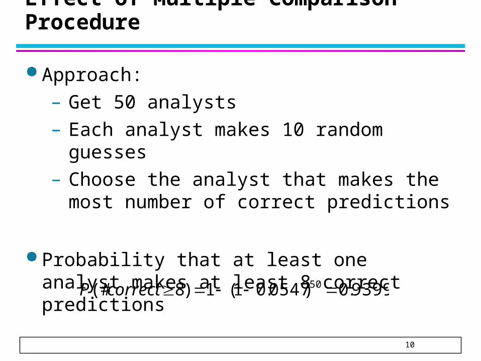
Pessimistic Estimate

+: 5-: 2

+: 1-: 4

+: 3-: 0

+: 3-: 6

+: 3-: 0

+: 0-: 5

+: 3-: 1

+: 1-: 2

+: 0-: 2

+: 2-: 1

+: 3-: 1

Decision Tree, TL Decision Tree, TR

e(TL) = 4/24

e(TR) = 6/24

= 1

e’(TL) = (4 +7 1)/24 = 0.458

e’(TR) = (6 + 4 1)/24 = 0.417

18

Minimum Description Length (MDL)

Cost(Model,Data) = Cost(Data|Model) + Cost(Model)– Cost is the number of bits needed for encoding.– Search for the least costly model.

Cost(Data|Model) encodes the misclassification errors. Cost(Model) uses node encoding (number of children)

plus splitting condition encoding.

A B

A?

B?

C?

10

0

1

Yes No

B1 B2

C1 C2

X yX1 1X2 0X3 0X4 1

… …Xn 1

X yX1 ?X2 ?X3 ?X4 ?

… …Xn ?

19

Estimating Statistical Bounds

+: 5-: 2

+: 2-: 1

+: 3-: 1

Before splitting: e = 2/7, e’(7, 2/7, 0.25) = 0.503

e’(T) = 7 0.503 = 3.521

After splitting:

e(TL) = 1/4, e’(4, 1/4, 0.25) = 0.537

e(TR) = 1/3, e’(3, 1/3, 0.25) = 0.650

e’(T) = 4 0.537 + 3 0.650 = 4.098

Nz

Nz

Nee

zN

ze

eNe 22/

2

22/

2/

22/

1

4)1(

2),,('

20

Using Validation Set

Divide training data into two parts:

– Training set: use for model building

– Validation set: use for estimating generalization error Note: validation set is not the same as test set

Drawback:

– Less data available for training

21

Handling Overfitting in Decision Tree

Pre-Pruning (Early Stopping Rule)

– Stop the algorithm before it becomes a fully-grown tree

– Typical stopping conditions for a node: Stop if all instances belong to the same class Stop if all the attribute values are the same

– More restrictive conditions: Stop if number of instances is less than some user-specified threshold Stop if class distribution of instances are independent of the available features (e.g., using 2 test) Stop if expanding the current node does not improve impurity measures (e.g., Gini or information gain). Stop if estimated generalization error falls below certain threshold

22

Handling Overfitting in Decision Tree

Post-pruning

– Grow decision tree to its entirety

– Subtree replacement Trim the nodes of the decision tree in a bottom-up fashion If generalization error improves after trimming, replace sub-tree by a leaf node Class label of leaf node is determined from majority class of instances in the sub-tree

– Subtree raising Replace subtree with most frequently used branch

23

Example of Post-Pruning

A?

A1

A2 A3

A4

Class = Yes 20

Class = No 10

Error = 10/30

Training Error (Before splitting) = 10/30

Pessimistic error = (10 + 0.5)/30 = 10.5/30

Training Error (After splitting) = 9/30

Pessimistic error (After splitting)

= (9 + 4 0.5)/30 = 11/30

PRUNE!

Class = Yes 8

Class = No 4

Class = Yes 3

Class = No 4

Class = Yes 4

Class = No 1

Class = Yes 5

Class = No 1

24

Examples of Post-pruning

Simplified Decision Tree:

depth = 1 :| ImagePages <= 0.1333 : class 1| ImagePages > 0.1333 :| | breadth <= 6 : class 0| | breadth > 6 : class 1depth > 1 :| MultiAgent = 0: class 0| MultiAgent = 1:| | totalPages <= 81 : class 0| | totalPages > 81 : class 1

Decision Tree:

depth = 1 :| breadth > 7 : class 1| breadth <= 7 :| | breadth <= 3 :| | | ImagePages > 0.375 : class 0| | | ImagePages <= 0.375 :| | | | totalPages <= 6 : class 1| | | | totalPages > 6 :| | | | | breadth <= 1 : class 1| | | | | breadth > 1 : class 0| | width > 3 :| | | MultiIP = 0:| | | | ImagePages <= 0.1333 : class 1| | | | ImagePages > 0.1333 :| | | | | breadth <= 6 : class 0| | | | | breadth > 6 : class 1| | | MultiIP = 1:| | | | TotalTime <= 361 : class 0| | | | TotalTime > 361 : class 1depth > 1 :| MultiAgent = 0:| | depth > 2 : class 0| | depth <= 2 :| | | MultiIP = 1: class 0| | | MultiIP = 0:| | | | breadth <= 6 : class 0| | | | breadth > 6 :| | | | | RepeatedAccess <= 0.0322 : class 0| | | | | RepeatedAccess > 0.0322 : class 1| MultiAgent = 1:| | totalPages <= 81 : class 0| | totalPages > 81 : class 1

SubtreeRaising

SubtreeReplacement

25

Evaluating Performance of Classifier

Model Selection– Performed during model building– Purpose is to ensure that model is not overly

complex (to avoid overfitting)– Need to estimate generalization error

Model Evaluation– Performed after model has been constructed– Purpose is to estimate performance of

classifier on previously unseen data (e.g., test set)

26

Methods for Classifier Evaluation

Holdout

– Reserve k% for training and (100-k)% for testing Random subsampling

– Repeated holdout Cross validation

– Partition data into k disjoint subsets

– k-fold: train on k-1 partitions, test on the remaining one

– Leave-one-out: k=n Bootstrap

– Sampling with replacement

– .632 bootstrap:

b

isiboot accacc

bacc

1

368.0632.01

27

Methods for Comparing Classifiers

Given two models:– Model M1: accuracy = 85%, tested on 30 instances

– Model M2: accuracy = 75%, tested on 5000 instances

Can we say M1 is better than M2?– How much confidence can we place on accuracy of M1

and M2?

– Can the difference in performance measure be explained as a result of random fluctuations in the test set?

28

Confidence Interval for Accuracy

Prediction can be regarded as a Bernoulli trial

– A Bernoulli trial has 2 possible outcomes Coin toss – head/tail Prediction – correct/wrong

– Collection of Bernoulli trials has a Binomial distribution: x Bin(N, p) x: number of correct predictions

Estimate number of events

– Given N and p, find P(x=k) or E(x)

– Example: Toss a fair coin 50 times, how many heads would turn up? Expected number of heads = Np = 50 0.5 = 25

29

Confidence Interval for Accuracy

Estimate parameter of distribution– Given x (# of correct predictions)

or equivalently, acc=x/N, and N (# of test instances),

– Find upper and lower bounds of p (true accuracy of model)

30

Confidence Interval for Accuracy

For large test sets (N > 30), – acc has a normal distribution

with mean p and variance p(1-p)/N

Confidence Interval for p:

1

)/)1(

(2/12/

ZNpp

paccZP

Area = 1 -

Z/2 Z1- /2

)(2

4422

2/

22

2/

2

2/

ZN

accNaccNZZaccNp

31

Confidence Interval for Accuracy

Consider a model that produces an accuracy of 80% when evaluated on 100 test instances:– N=100, acc = 0.8

– Let 1- = 0.95 (95% confidence)

– From probability table, Z/2=1.96

1- Z

0.99 2.58

0.98 2.33

0.95 1.96

0.90 1.65

N 50 100 500 1000 5000

p(lower) 0.670 0.711 0.763 0.774 0.789

p(upper) 0.888 0.866 0.833 0.824 0.811

32

Comparing Performance of 2 Models

Given two models, say M1 and M2, which is better?– M1 is tested on D1 (size=n1), found error rate = e1

– M2 is tested on D2 (size=n2), found error rate = e2

– Assume D1 and D2 are independent

– If n1 and n2 are sufficiently large, then

– Approximate:

222

111

,~

,~

Ne

Ne

i

ii

i nee )1(

ˆ

33

Comparing Performance of 2 Models

To test if performance difference is statistically significant: d = e1 – e2– d ~ NN(dt,t) where dt is the true difference

– Since D1 and D2 are independent, their variance adds up:

– At (1-) confidence level,

2)21(2

1)11(1

ˆˆ 2

2

2

1

2

2

2

1

2

nee

nee

t

ttZdd

ˆ

2/

34

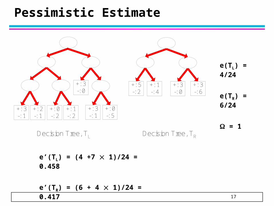
An Illustrative Example

Given: M1: n1 = 30, e1 = 0.15 M2: n2 = 5000, e2 = 0.25

d = |e2 – e1| = 0.1 (2-sided test)

At 95% confidence level, Z/2=1.96

=> Interval contains 0 => difference may not be statistically significant

0043.05000

)25.01(25.030

)15.01(15.0ˆ

d

128.0100.00043.096.1100.0 t

d

35

Comparing Performance of 2 Classifiers

Each classifier produces k models:– C1 may produce M11 , M12, …, M1k

– C2 may produce M21 , M22, …, M2k

If models are applied to the same test sets D1,D2, …, Dk (e.g., via cross-validation)– For each set: compute dj = e1j – e2j

– dj has mean d and variance t2

– Estimate:

tkt

k

jj

t

tdd

kk

dd

ˆ

)1(

)(

ˆ

1,1

1

2

2

36

An Illustrative Example

30-fold cross validation:

– Average difference = 0.05

– Std deviation of difference = 0.002

At 95% confidence level, t = 2.04

– Interval does not span the value 0, so difference is statistically significant

00408.005.0002.004.205.0 td