1 Correspondence Analysis Correspondence analysis is a descriptive/exploratory technique designed to analyse simple two-way and multi-way tables containing

1

Correspondence Analysis

Correspondence analysis is a descriptive/exploratory technique designed to analyse simple two-way and multi-way tables containing some measure of correspondence between the rows and columns.

The results provide information which is similar in nature to those produced by Factor Analysis techniques, and they allow one to explore the structure of categorical variables included in the table. The most common kind of table of this type is the two-way frequency cross-tabulation table.

Tuesday 18 April 2023 08:52 PM

2


Correspondence analysis (CA) may be defined as a special case of principal components analysis (PCA) of the rows and columns of a table, especially applicable to a cross-tabulation. However CA and PCA are used under different circumstances. Principal components analysis is used for tables consisting of continuous measurement, whereas correspondence analysis is applied to contingency tables (i.e. cross-tabulations). Its primary goal is to transform a table of numerical information into a graphical display, in which each row and each column is depicted as a point.

3


In a typical correspondence analysis, a cross-tabulation table of frequencies is first standardised, so that the relative frequencies across all cells sum to 1.0.

One way to state the goal of a typical analysis is to represent the entries in the table of relative frequencies in terms of the distances between individual rows and/or columns in a low-dimensional space.

There are several parallels in interpretation between correspondence analysis and factor analysis.

4


Correspondence Analysis Applied to Psychological Research

L. Doey and J. Kurta

Tutorials in Quantitative Methods for Psychology

2011, Vol. 7(1)7(1), p. 5-14.

http://www.tqmp.org/Content/vol07-1/p005/p005.pdf

http://www.tqmp.org/Content/vol07-1/p005/p005.pdf

5


An Introduction to Correspondence Analysis

P.M. Yelland

The Mathematica Journal 2010, Vol. 1212, p. 1-23.

http://www.mathematica-journal.com/data/uploads/2010/09/Yelland.pdf

http://www.mathematica-journal.com/data/uploads/2010/09/Yelland.pdf

6


Correspondence analysis is a useful tool to uncover the relationships among categorical variables

N. Sourial, C. Wolfson, B. Zhu, J. Quail, J. Fletcher, S. Karunananthan, K. Bandeen-Roche, F. Béland and H. Bergman

Journal of Clinical Epidemiology 2010

Volume 63, Issue 6, Pages 638-646

http://www.sciencedirect.com/science/article/pii/S0895435609002376

http://www.sciencedirect.com/science/article/pii/S0895435609002376

7


The data summarises individuals political affiliation (1,…,5) and geographic region (1,…,4) .

1 Liberal

2 Tend Lib

3 Moderate

4 Tend Cons

5 Conservative

8


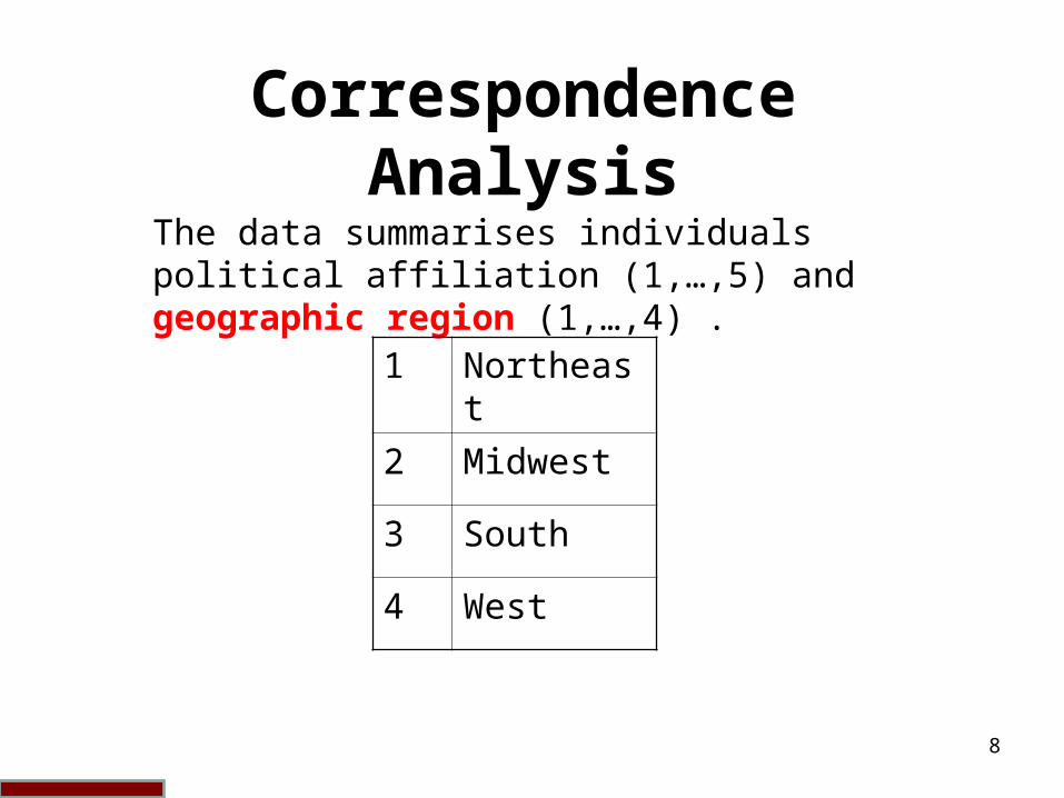
The data summarises individuals political affiliation (1,…,5) and geographic region (1,…,4) .

1 Northeast

2 Midwest

3 South

4 West

9


The data (a) summarises individuals political affiliation (1,…,5) and geographic region (1,…,4) .

725 rows of data

10


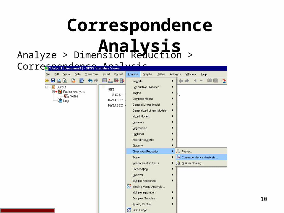
Analyze > Dimension Reduction > Correspondence Analysis

11


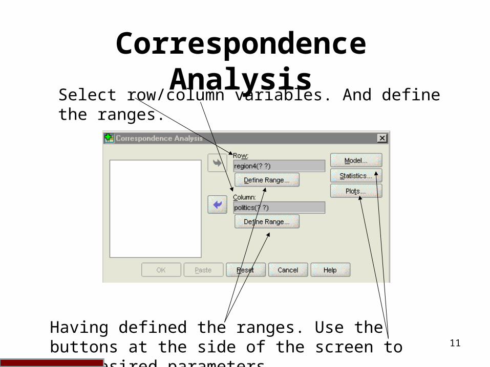
Select row/column variables. And define the ranges.

Having defined the ranges. Use the buttons at the side of the screen to set desired parameters.

12


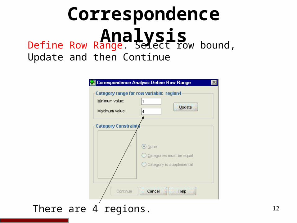
Define Row Range. Select row bound, Update and then Continue

There are 4 regions.

13


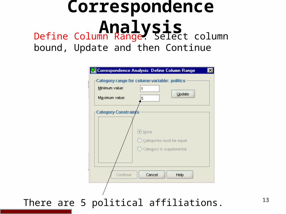
Define Column Range. Select column bound, Update and then Continue

There are 5 political affiliations.

14


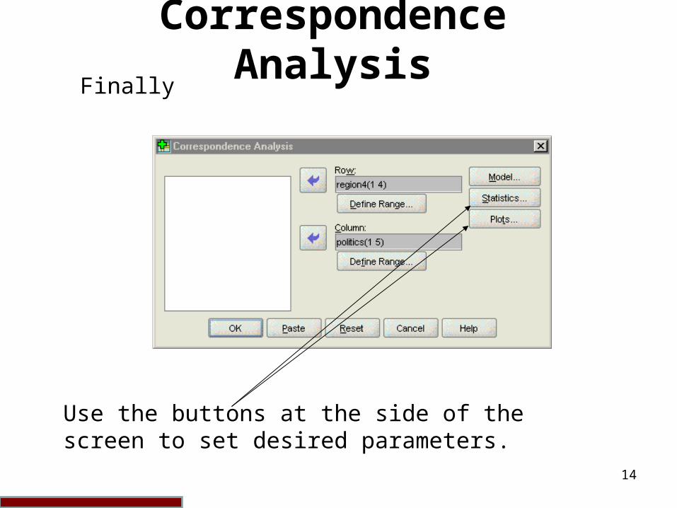
Finally

Use the buttons at the side of the screen to set desired parameters.

15


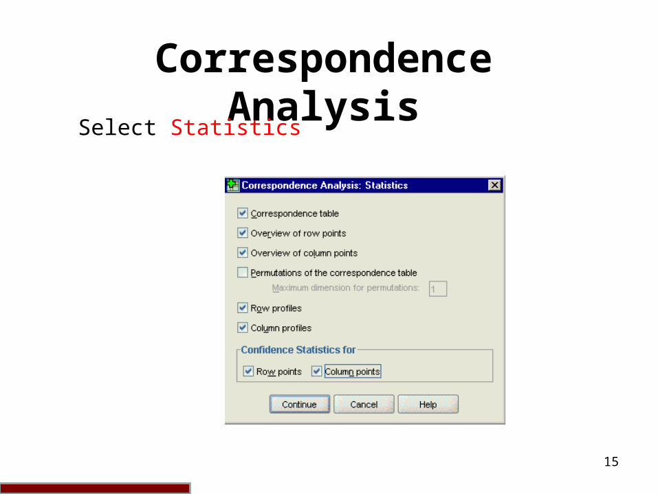
Select Statistics

16


Select Plots

17


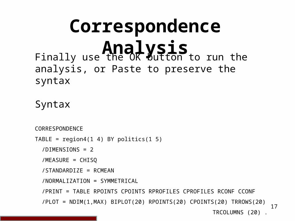
Finally use the OK button to run the analysis, or Paste to preserve the syntax

Syntax

CORRESPONDENCE

TABLE = region4(1 4) BY politics(1 5)

/DIMENSIONS = 2

/MEASURE = CHISQ

/STANDARDIZE = RCMEAN

/NORMALIZATION = SYMMETRICAL

/PRINT = TABLE RPOINTS CPOINTS RPROFILES CPROFILES RCONF CCONF

/PLOT = NDIM(1,MAX) BIPLOT(20) RPOINTS(20) CPOINTS(20) TRROWS(20)

TRCOLUMNS (20) .

18


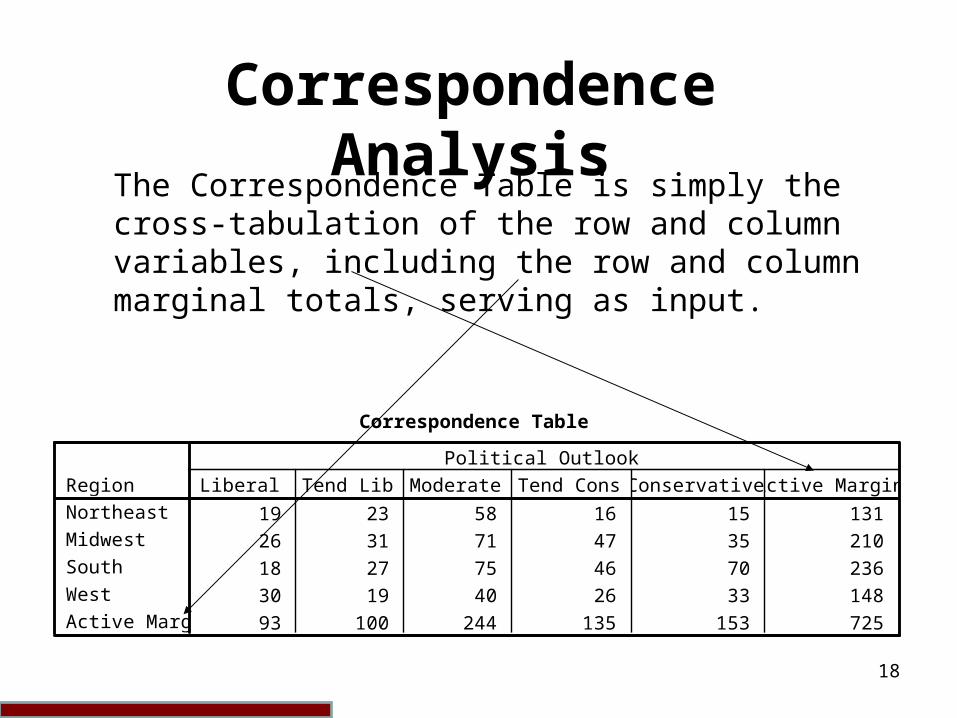
The Correspondence Table is simply the cross-tabulation of the row and column variables, including the row and column marginal totals, serving as input.

Correspondence Table

19 23 58 16 15 131

26 31 71 47 35 210

18 27 75 46 70 236

30 19 40 26 33 148

93 100 244 135 153 725

RegionNortheast

Midwest

South

West

Active Margin

Liberal Tend Lib Moderate Tend Cons Conservative Active Margin

Political Outlook

19


The Row Profiles are the cell contents divided by their corresponding row total (eg. 19/131=0.145 for the first cell). This table also shows the column masses (column marginals as a percent of n) (eg. 93/725=0.128). These are intermediate calculations on the way toward computing distances between points. Note the column of 1’s.

Row Profiles

.145 .176 .443 .122 .115 1.000

.124 .148 .338 .224 .167 1.000

.076 .114 .318 .195 .297 1.000

.203 .128 .270 .176 .223 1.000

.128 .138 .337 .186 .211

RegionNortheast

Midwest

South

West

Mass

Liberal Tend Lib Moderate Tend Cons Conservative Active Margin

Political Outlook

20


Column Profiles are the cell elements divided by the column marginals (ex. 19/103=0.204). This table also shows the row masses (row marginals as a percent of n) (ex. 131/725=0.181). These are intermediate calculations on the way toward computing distances between points. Note the row of 1’s.

Column Profiles

.204 .230 .238 .119 .098 .181

.280 .310 .291 .348 .229 .290

.194 .270 .307 .341 .458 .326

.323 .190 .164 .193 .216 .204

1.000 1.000 1.000 1.000 1.000

RegionNortheast

Midwest

South

West

Active Margin

Liberal Tend Lib Moderate Tend Cons Conservative Mass

Political Outlook

21


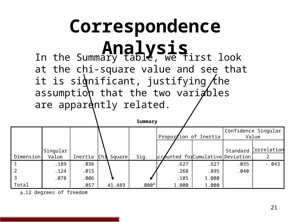
In the Summary table, we first look at the chi‑square value and see that it is significant, justifying the assumption that the two variables are apparently related.

Summary

.189 .036 .627 .627 .035 -.043

.124 .015 .268 .895 .040

.078 .006 .105 1.000

.057 41.489 .000a 1.000 1.000

Dimension1

2

3

Total

SingularValue Inertia Chi Square Sig. Accounted for Cumulative

Proportion of Inertia

StandardDeviation 2

Correlation

Confidence SingularValue

12 degrees of freedoma.

22


SPSS has computed the interpoint distances and subjected the distance matrix to principal components analysis, yielding in this case three dimensions.

Summary

.189 .036 .627 .627 .035 -.043

.124 .015 .268 .895 .040

.078 .006 .105 1.000

.057 41.489 .000a 1.000 1.000

Dimension1

2

3

Total



StandardDeviation 2

Correlation



23


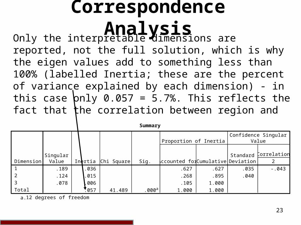
Only the interpretable dimensions are reported, not the full solution, which is why the eigen values add to something less than 100% (labelled Inertia; these are the percent of variance explained by each dimension) - in this case only 0.057 = 5.7%. This reflects the fact that the correlation between region and political outlook, while significant, is weak.

Summary

.189 .036 .627 .627 .035 -.043

.124 .015 .268 .895 .040

.078 .006 .105 1.000

.057 41.489 .000a 1.000 1.000

Dimension1

2

3

Total



StandardDeviation 2

Correlation



24


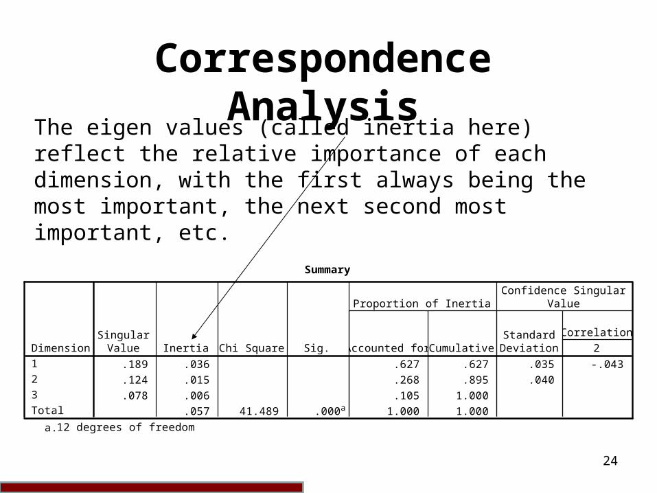
The eigen values (called inertia here) reflect the relative importance of each dimension, with the first always being the most important, the next second most important, etc.

Summary

.189 .036 .627 .627 .035 -.043

.124 .015 .268 .895 .040

.078 .006 .105 1.000

.057 41.489 .000a 1.000 1.000

Dimension1

2

3

Total



StandardDeviation 2

Correlation



25


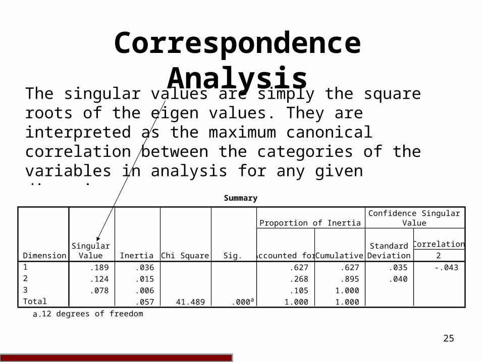
The singular values are simply the square roots of the eigen values. They are interpreted as the maximum canonical correlation between the categories of the variables in analysis for any given dimension.

Summary

.189 .036 .627 .627 .035 -.043

.124 .015 .268 .895 .040

.078 .006 .105 1.000

.057 41.489 .000a 1.000 1.000

Dimension1

2

3

Total



StandardDeviation 2

Correlation



26


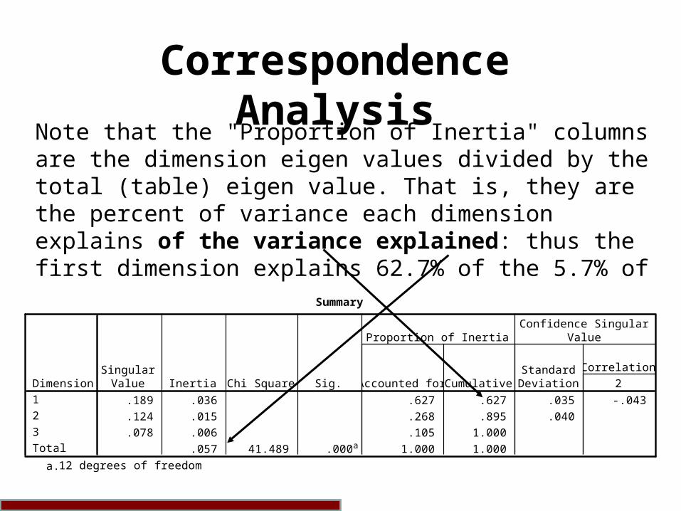
Note that the "Proportion of Inertia" columns are the dimension eigen values divided by the total (table) eigen value. That is, they are the percent of variance each dimension explains of the variance explained: thus the first dimension explains 62.7% of the 5.7% of the variance explained by the model.

Summary

.189 .036 .627 .627 .035 -.043

.124 .015 .268 .895 .040

.078 .006 .105 1.000

.057 41.489 .000a 1.000 1.000

Dimension1

2

3

Total



StandardDeviation 2

Correlation



27


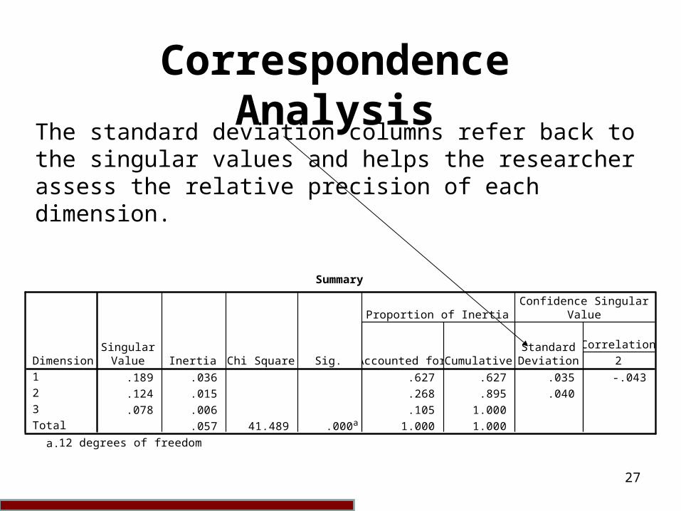
The standard deviation columns refer back to the singular values and helps the researcher assess the relative precision of each dimension.

Summary

.189 .036 .627 .627 .035 -.043

.124 .015 .268 .895 .040

.078 .006 .105 1.000

.057 41.489 .000a 1.000 1.000

Dimension1

2

3

Total



StandardDeviation 2

Correlation



28


Keyword interpretations

Mass: the marginal proportions of the row variable, used to weight the point profiles when computing point distance. This weighting has the effect of compensating for unequal numbers of cases.

Scores in dimension: scores used as coordinates for points when plotting the correspondence map. Each point has a score on each dimension.

Inertia: Variance

29


Contribution of points to dimensions: as factor loadings are used in conventional factor analysis to ascribe meaning to dimensions, so "contribution of points to dimensions" is used to intuit the meaning of correspondence dimensions.

Contribution of dimensions to points: these are multiple correlations, which reflect how well the principal components model is explaining any given point (category).

30


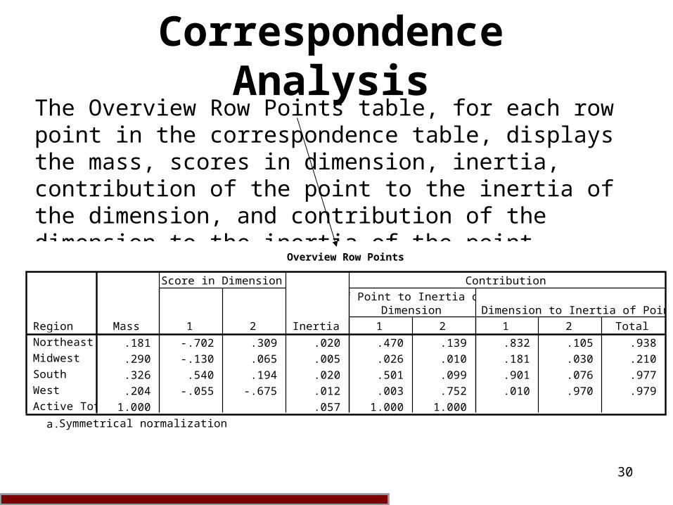
The Overview Row Points table, for each row point in the correspondence table, displays the mass, scores in dimension, inertia, contribution of the point to the inertia of the dimension, and contribution of the dimension to the inertia of the point.

Overview Row Pointsa

.181 -.702 .309 .020 .470 .139 .832 .105 .938

.290 -.130 .065 .005 .026 .010 .181 .030 .210

.326 .540 .194 .020 .501 .099 .901 .076 .977

.204 -.055 -.675 .012 .003 .752 .010 .970 .979

1.000 .057 1.000 1.000

RegionNortheast

Midwest

South

West

Active Total

Mass 1 2

Score in Dimension

Inertia 1 2

Of Point to Inertia ofDimension

1 2 Total

Of Dimension to Inertia of Point

Contribution

Symmetrical normalizationa.

Overview Row Points

31


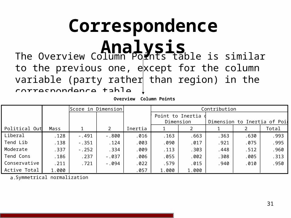
The Overview Column Points table is similar to the previous one, except for the column variable (party rather than region) in the correspondence table.

Overview Column Pointsa

.128 -.491 -.800 .016 .163 .663 .363 .630 .993

.138 -.351 .124 .003 .090 .017 .921 .075 .995

.337 -.252 .334 .009 .113 .303 .448 .512 .960

.186 .237 -.037 .006 .055 .002 .308 .005 .313

.211 .721 -.094 .022 .579 .015 .940 .010 .950

1.000 .057 1.000 1.000

Political OutlookLiberal

Tend Lib

Moderate

Tend Cons

Conservative

Active Total

Mass 1 2

Score in Dimension

Inertia 1 2

Of Point to Inertia ofDimension

1 2 Total

Of Dimension to Inertia of Point

Contribution

Symmetrical normalizationa.

Overview Column Points

32


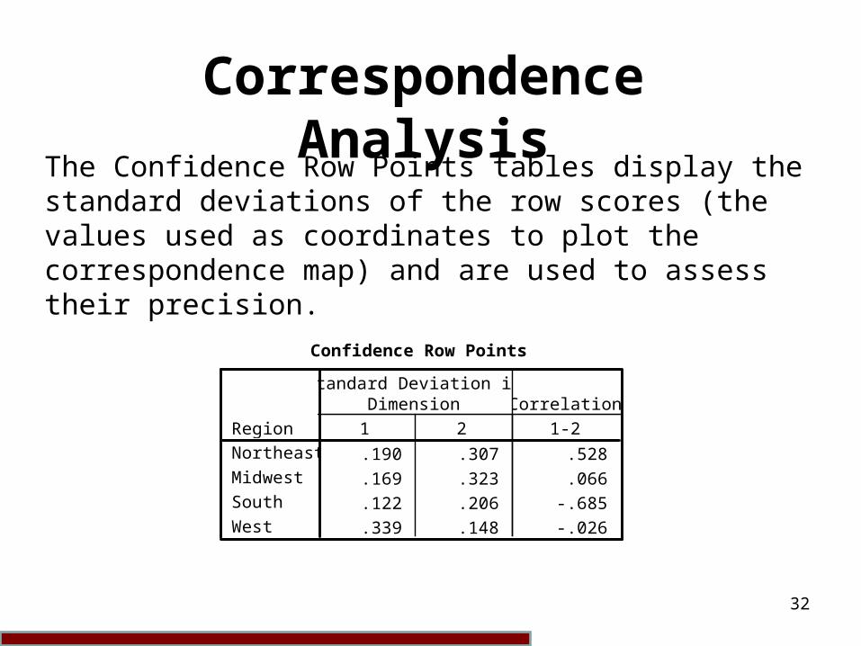
The Confidence Row Points tables display the standard deviations of the row scores (the values used as coordinates to plot the correspondence map) and are used to assess their precision.

Confidence Row Points

.190 .307 .528

.169 .323 .066

.122 .206 -.685

.339 .148 -.026

RegionNortheast

Midwest

South

West

1 2

Standard Deviation inDimension

1-2

Correlation

33


The Confidence Column Points tables display the standard deviations of the column scores (the values used as coordinates to plot the correspondence map) and are used to assess their precision.

Confidence Column Points

.387 .221 -.694

.072 .117 .801

.171 .122 .575

.215 .406 .095

.127 .302 .304

Political OutlookLiberal

Tend Lib

Moderate

Tend Cons

Conservative

1 2

Standard Deviation inDimension

1-2

Correlation

34


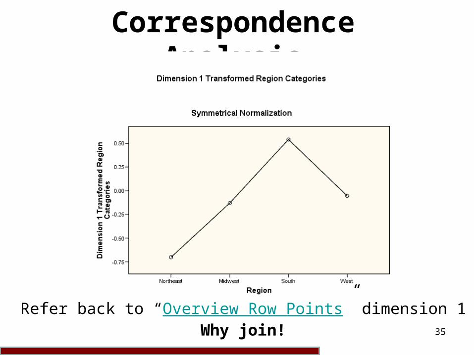
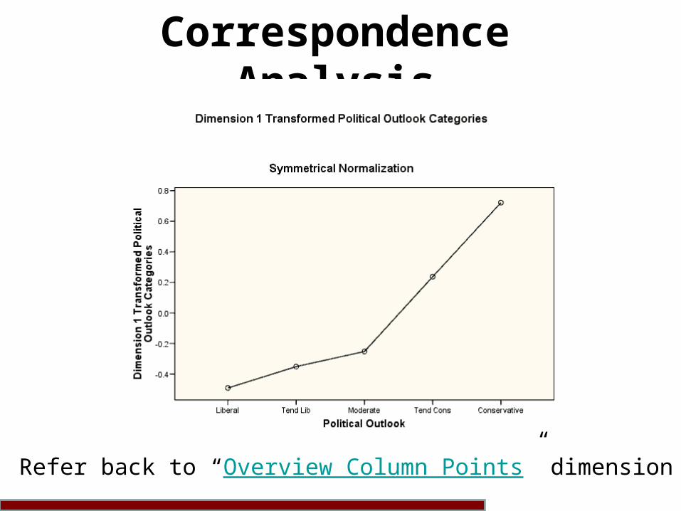
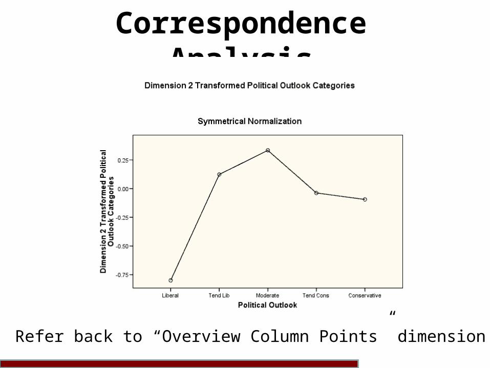
The plots of transformed categories for dimensions display a plot of the transformation of the row category values and of column category values into scores in dimension, with one plot per dimension.

The x-axis has the category values and the y-axis has the corresponding dimension scores. Thus the category "Northeast" in the Overview Row Points table above had a score in dimension of -0.702, as shown on the plot.

35


Refer back to “Overview Row Points” dimension 1Why join!

36


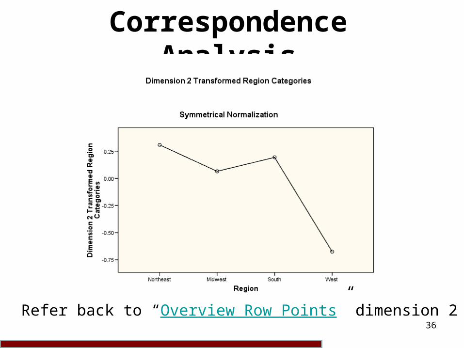
Refer back to “Overview Row Points” dimension 2

37


Refer back to “Overview Column Points” dimension 1

38


Refer back to “Overview Column Points” dimension 2

39


The uniplots for the row and column variables. Note that the origin of the axes is slightly different in the two plots.

40


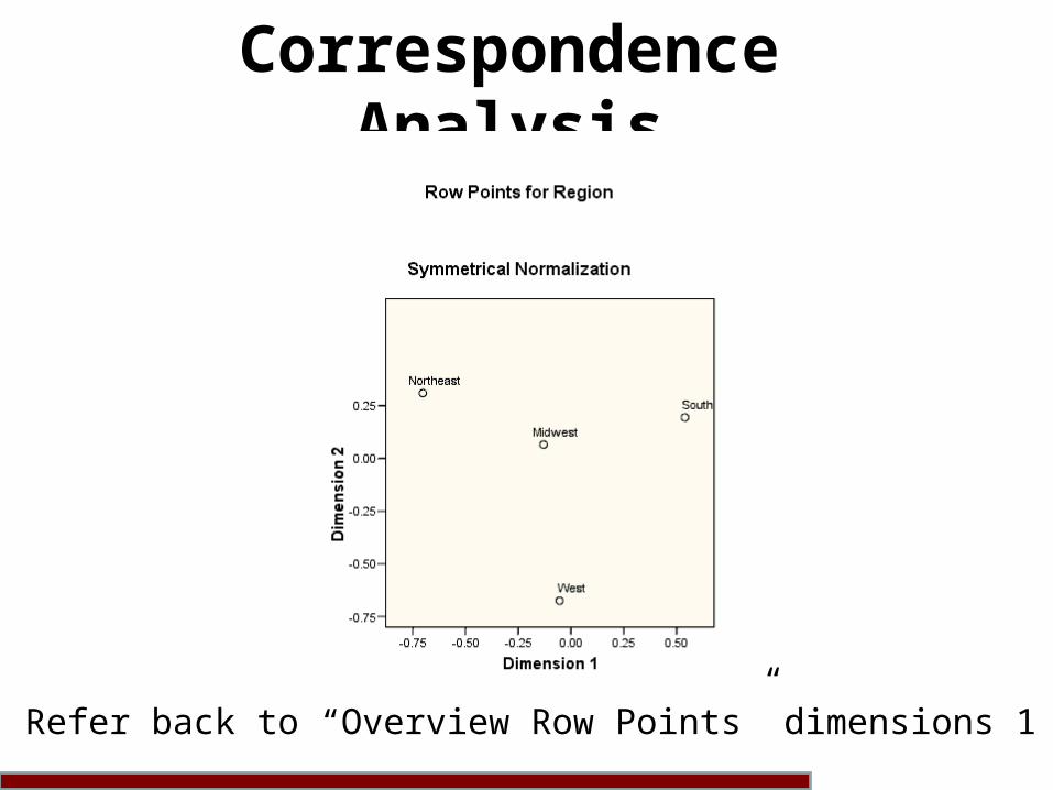
Refer back to “Overview Row Points” dimensions 1 & 2

41


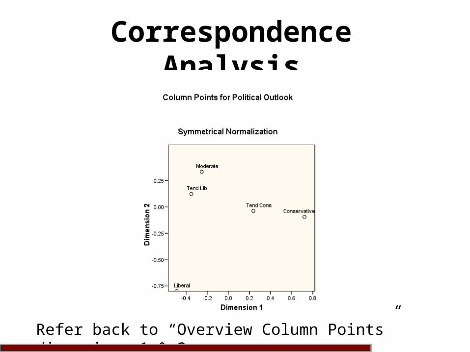
Refer back to “Overview Column Points” dimensions 1 & 2

42


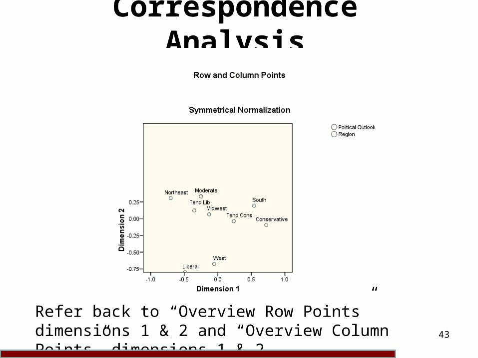
Finally the biplot correspondence map is obtained.

Note the axes now encompass the most extreme values of both of the uniplots.

Note that while some generalizations can be made about the association of categories (South more conservative, West more liberal). The researcher must keep firmly in mind that correspondence is not association. That is, the researcher should not allow the maps display of inter-category distances to obscure the fact that, for this example, the model only explains 5.7% of the variance in the correspondence table.

43


Refer back to “Overview Row Points” dimensions 1 & 2 and “Overview Column Points” dimensions 1 & 2.

44

Correspondence AnalysisCare must be taken when interpreting the

previous plot. It must be remembered that distances between columns and rows are not defined.

“Symmetrical normalization (via the model button slide) is a technique used to standardize row and column data so as to be able to make general comparisons between the two. Other forms of standardization allow you to compare row variable points or column variable points, or rows or columns, but not rows to columns (see Garson, 2012 for further information on other standardization techniques for correspondence analysis).” Doey and Kurta 2011 (slide)

45


Input Of A Collated Data Matrix

An SPSS program that will do this operation is ANACOR, although since we are using data in table form, this has to be performed using the command syntax window.

46


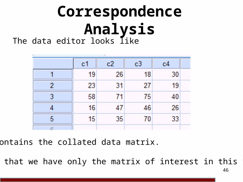
The data editor looks like

It contains the collated data matrix.

Note that we have only the matrix of interest in this view.

47


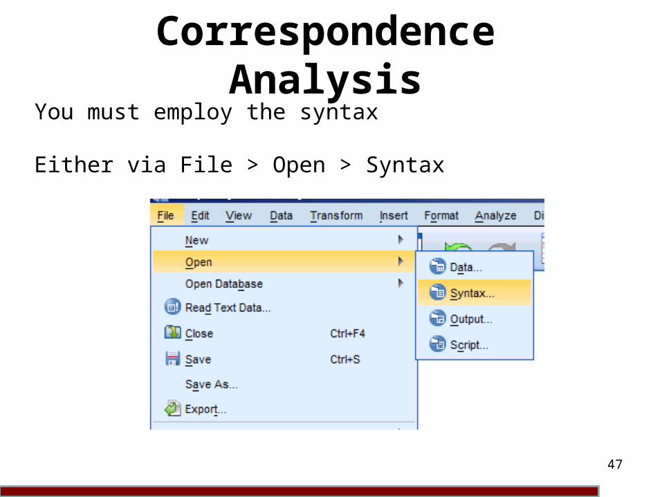
You must employ the syntax

Either via File > Open > Syntax

48


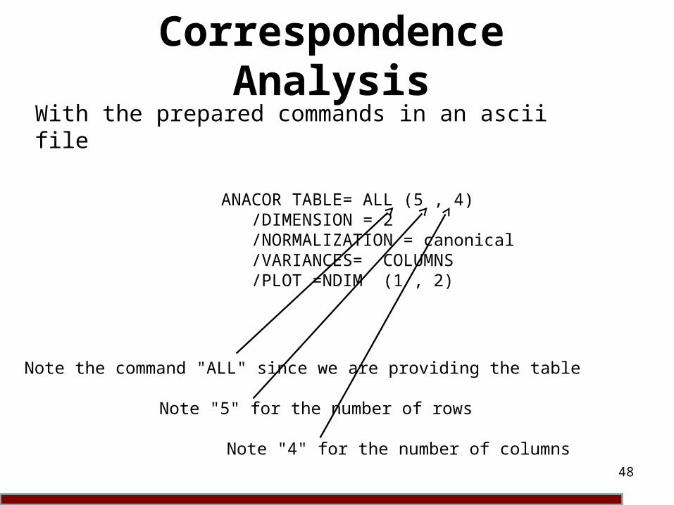
With the prepared commands in an ascii file

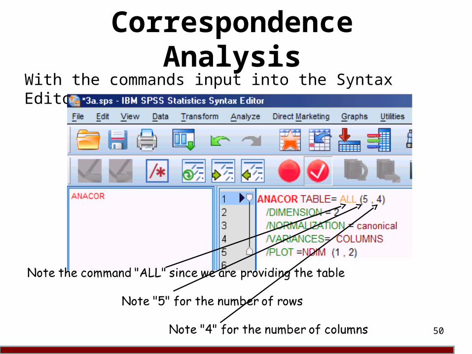
ANACOR TABLE= ALL (5 , 4) /DIMENSION = 2 /NORMALIZATION = canonical /VARIANCES= COLUMNS /PLOT =NDIM (1 , 2)

Note the command "ALL" since we are providing the table

Note "5" for the number of rows

Note "4" for the number of columns

49


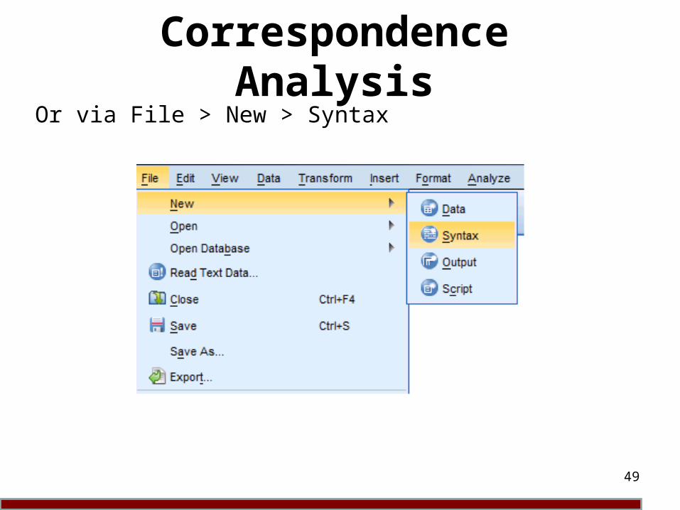
Or via File > New > Syntax

50


With the commands input into the Syntax Editor

51


The solution is, of course, unchanged.

52

SPSS Tips

Now you should go and try for yourself.

Each week our cluster (5.05) is booked for 2 hours after this session. This will enable you to come and go as you please.

Obviously other timetabled sessions for this module take precedence..

Documents

1 Correspondence Analysis Correspondence analysis is a descriptive/exploratory technique designed to analyse simple two-way and multi-way tables containing