1

Computer Graphics & Image Processing

�How many lectures are there?u Four this termu Twelve next term

�Who gets examined on it?u Part IBu Part II (General)u Diploma

2What are Computer Graphics &Image Processing?

Scenedescription

Digitalimage

Computergraphics

Image analysis &computer vision

Image processing

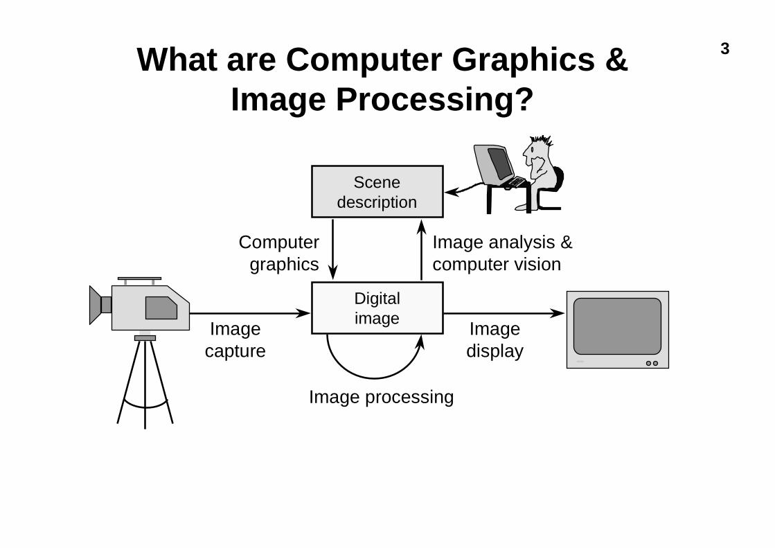
3What are Computer Graphics &Image Processing?

Scenedescription

Digitalimage

Computergraphics

Image analysis &computer vision

Image processing

Imagecapture

Imagedisplay

4

Why bother with CG & IP?

�all visual computer output depends onComputer Graphicsu printed outputu monitor (CRT/LCD/whatever)u all visual computer output consists of real images

generated by the computer from some internaldigital image

5

What are CG & IP used for?u 2D computer graphics

n graphical user interfaces: Mac, Windows, X,…n graphic design: posters, cereal packets,…n typesetting: book publishing, report writing,…

u Image processingn photograph retouching: publishing, posters,…n photocollaging: satellite imagery,…n art: new forms of artwork based on digitised images

u 3D computer graphicsn visualisation: scientific, medical, architectural,…n Computer Aided Design (CAD)n entertainment: special effect, games, movies,…

6

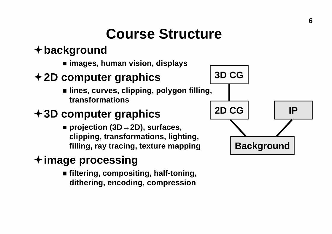
Course Structure�background

n images, human vision, displays

�2D computer graphicsn lines, curves, clipping, polygon filling,

transformations

�3D computer graphicsn projection (3D→2D), surfaces,

clipping, transformations, lighting,filling, ray tracing, texture mapping

�image processingn filtering, compositing, half-toning,

dithering, encoding, compression

Background

2D CG IP

3D CG

7

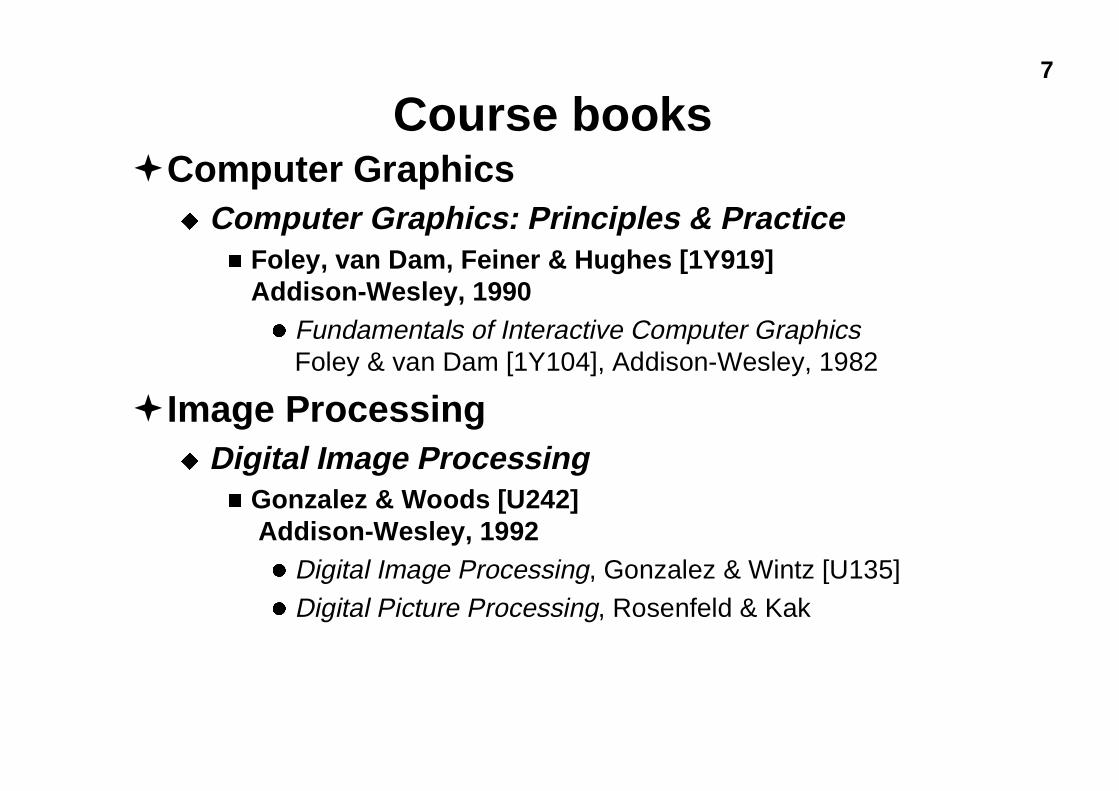
Course books�Computer Graphics

u Computer Graphics: Principles & Practicen Foley, van Dam, Feiner & Hughes [1Y919]

Addison-Wesley, 1990l Fundamentals of Interactive Computer Graphics

Foley & van Dam [1Y104], Addison-Wesley, 1982

�Image Processingu Digital Image Processing

n Gonzalez & Woods [U242] Addison-Wesley, 1992l Digital Image Processing, Gonzalez & Wintz [U135]

l Digital Picture Processing, Rosenfeld & Kak

8

Past exam questionsu 98/4/10ä 98/5/4ä 98/6/4ä (11/11,12/4,13/4)u 97/4/10ä 97/5/2? 97/6/4ä (11/11,12/2,13/4)u 96/4/10? 96/5/4ä 96/6/4ä (11/11,12/4,13/4)u 95/4/8ä 95/5/4ä 95/6/4ä (11/9,12/4,13/4)u 94/3/8? 94/4/8? 94/5/4? 94/6/4? (10/9,11/8,12/4,13/4)u 93/3/9ã 93/4/9? 93/5/4ã 93/6/4ã (10/9,11/9,12/4,13/4)

ä could be set exactly as it is? could be set in a different form or parts could be setã would not be set

n N.B. Diploma/Part II(G) questions in parentheses are identicalto the corresponding Part IB questions

9

Background

�what is a digital image?u what are the constraints on digital images?

�how does human vision work?u what are the limits of human vision?u what can we get away with given these constraints

& limits?

�how do displays & printers work?u how do we fool the human eye into seeing what we

want it to see?

2D CG IP

3D CG

Background

10

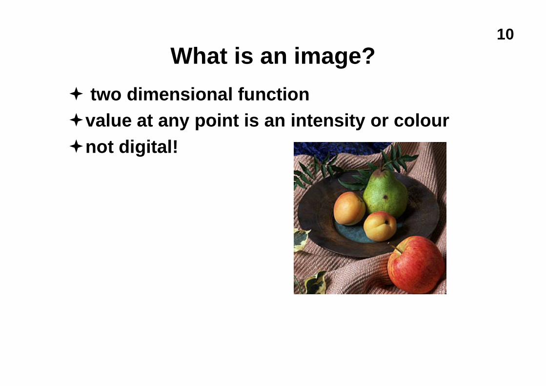
What is an image?

� two dimensional function�value at any point is an intensity or colour�not digital!

11

What is a digital image?

� a contradiction in termsu if you can see it, it’s not digitalu if it’s digital, it’s just a collection of numbers

�a sampled and quantised version of a realimage

�a rectangular array of intensity or colourvalues

12

Image capture

� a variety of devices can be usedu scanners

n line CCD in a flatbed scannern spot detector in a drum scanner

u camerasn area CCD

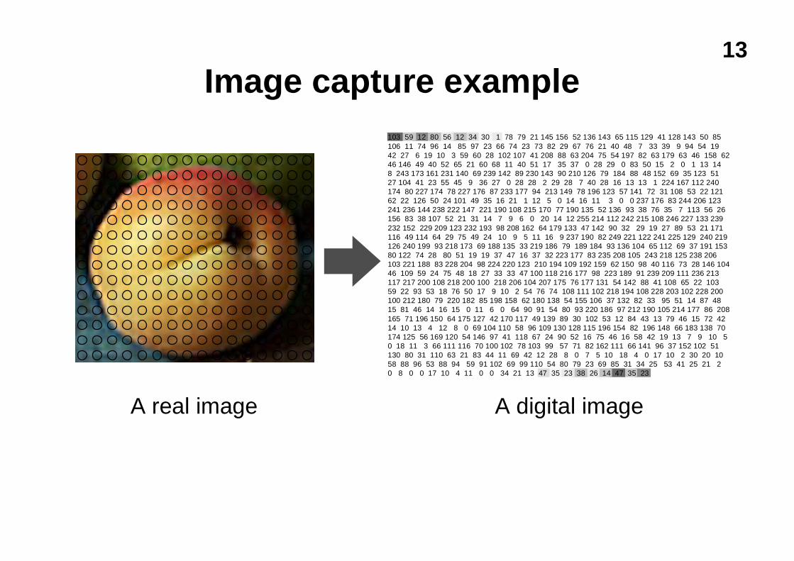
13

Image capture example

A real image A digital image

103 59 12 80 56 12 34 30 1 78 79 21 145 156 52 136 143 65 115 129 41 128 143 50 85106 11 74 96 14 85 97 23 66 74 23 73 82 29 67 76 21 40 48 7 33 39 9 94 54 1942 27 6 19 10 3 59 60 28 102 107 41 208 88 63 204 75 54 197 82 63 179 63 46 158 6246 146 49 40 52 65 21 60 68 11 40 51 17 35 37 0 28 29 0 83 50 15 2 0 1 13 148 243 173 161 231 140 69 239 142 89 230 143 90 210 126 79 184 88 48 152 69 35 123 5127 104 41 23 55 45 9 36 27 0 28 28 2 29 28 7 40 28 16 13 13 1 224 167 112 240174 80 227 174 78 227 176 87 233 177 94 213 149 78 196 123 57 141 72 31 108 53 22 12162 22 126 50 24 101 49 35 16 21 1 12 5 0 14 16 11 3 0 0 237 176 83 244 206 123241 236 144 238 222 147 221 190 108 215 170 77 190 135 52 136 93 38 76 35 7 113 56 26156 83 38 107 52 21 31 14 7 9 6 0 20 14 12 255 214 112 242 215 108 246 227 133 239232 152 229 209 123 232 193 98 208 162 64 179 133 47 142 90 32 29 19 27 89 53 21 171116 49 114 64 29 75 49 24 10 9 5 11 16 9 237 190 82 249 221 122 241 225 129 240 219126 240 199 93 218 173 69 188 135 33 219 186 79 189 184 93 136 104 65 112 69 37 191 15380 122 74 28 80 51 19 19 37 47 16 37 32 223 177 83 235 208 105 243 218 125 238 206103 221 188 83 228 204 98 224 220 123 210 194 109 192 159 62 150 98 40 116 73 28 146 10446 109 59 24 75 48 18 27 33 33 47 100 118 216 177 98 223 189 91 239 209 111 236 213117 217 200 108 218 200 100 218 206 104 207 175 76 177 131 54 142 88 41 108 65 22 10359 22 93 53 18 76 50 17 9 10 2 54 76 74 108 111 102 218 194 108 228 203 102 228 200100 212 180 79 220 182 85 198 158 62 180 138 54 155 106 37 132 82 33 95 51 14 87 4815 81 46 14 16 15 0 11 6 0 64 90 91 54 80 93 220 186 97 212 190 105 214 177 86 208165 71 196 150 64 175 127 42 170 117 49 139 89 30 102 53 12 84 43 13 79 46 15 72 4214 10 13 4 12 8 0 69 104 110 58 96 109 130 128 115 196 154 82 196 148 66 183 138 70174 125 56 169 120 54 146 97 41 118 67 24 90 52 16 75 46 16 58 42 19 13 7 9 10 50 18 11 3 66 111 116 70 100 102 78 103 99 57 71 82 162 111 66 141 96 37 152 102 51130 80 31 110 63 21 83 44 11 69 42 12 28 8 0 7 5 10 18 4 0 17 10 2 30 20 1058 88 96 53 88 94 59 91 102 69 99 110 54 80 79 23 69 85 31 34 25 53 41 25 21 20 8 0 0 17 10 4 11 0 0 34 21 13 47 35 23 38 26 14 47 35 23

14

Image display

�a digital image is an array of integers, how doyou display it?

�reconstruct a real image on some sort ofdisplay deviceu CRT - computer monitor, TV setu LCD - portable computeru printer - dot matrix, laser printer, dye sublimation

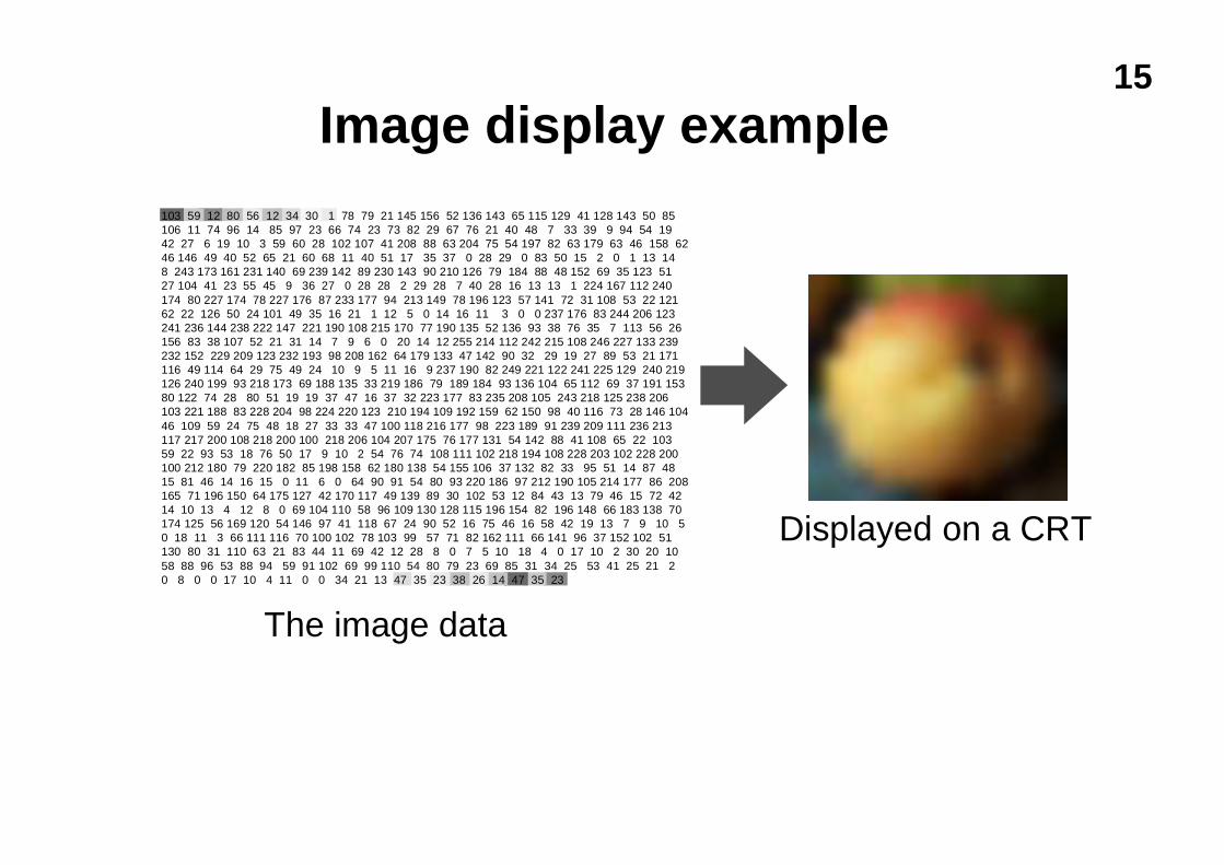
15

Image display example

Displayed on a CRT

The image data

103 59 12 80 56 12 34 30 1 78 79 21 145 156 52 136 143 65 115 129 41 128 143 50 85106 11 74 96 14 85 97 23 66 74 23 73 82 29 67 76 21 40 48 7 33 39 9 94 54 1942 27 6 19 10 3 59 60 28 102 107 41 208 88 63 204 75 54 197 82 63 179 63 46 158 6246 146 49 40 52 65 21 60 68 11 40 51 17 35 37 0 28 29 0 83 50 15 2 0 1 13 148 243 173 161 231 140 69 239 142 89 230 143 90 210 126 79 184 88 48 152 69 35 123 5127 104 41 23 55 45 9 36 27 0 28 28 2 29 28 7 40 28 16 13 13 1 224 167 112 240174 80 227 174 78 227 176 87 233 177 94 213 149 78 196 123 57 141 72 31 108 53 22 12162 22 126 50 24 101 49 35 16 21 1 12 5 0 14 16 11 3 0 0 237 176 83 244 206 123241 236 144 238 222 147 221 190 108 215 170 77 190 135 52 136 93 38 76 35 7 113 56 26156 83 38 107 52 21 31 14 7 9 6 0 20 14 12 255 214 112 242 215 108 246 227 133 239232 152 229 209 123 232 193 98 208 162 64 179 133 47 142 90 32 29 19 27 89 53 21 171116 49 114 64 29 75 49 24 10 9 5 11 16 9 237 190 82 249 221 122 241 225 129 240 219126 240 199 93 218 173 69 188 135 33 219 186 79 189 184 93 136 104 65 112 69 37 191 15380 122 74 28 80 51 19 19 37 47 16 37 32 223 177 83 235 208 105 243 218 125 238 206103 221 188 83 228 204 98 224 220 123 210 194 109 192 159 62 150 98 40 116 73 28 146 10446 109 59 24 75 48 18 27 33 33 47 100 118 216 177 98 223 189 91 239 209 111 236 213117 217 200 108 218 200 100 218 206 104 207 175 76 177 131 54 142 88 41 108 65 22 10359 22 93 53 18 76 50 17 9 10 2 54 76 74 108 111 102 218 194 108 228 203 102 228 200100 212 180 79 220 182 85 198 158 62 180 138 54 155 106 37 132 82 33 95 51 14 87 4815 81 46 14 16 15 0 11 6 0 64 90 91 54 80 93 220 186 97 212 190 105 214 177 86 208165 71 196 150 64 175 127 42 170 117 49 139 89 30 102 53 12 84 43 13 79 46 15 72 4214 10 13 4 12 8 0 69 104 110 58 96 109 130 128 115 196 154 82 196 148 66 183 138 70174 125 56 169 120 54 146 97 41 118 67 24 90 52 16 75 46 16 58 42 19 13 7 9 10 50 18 11 3 66 111 116 70 100 102 78 103 99 57 71 82 162 111 66 141 96 37 152 102 51130 80 31 110 63 21 83 44 11 69 42 12 28 8 0 7 5 10 18 4 0 17 10 2 30 20 1058 88 96 53 88 94 59 91 102 69 99 110 54 80 79 23 69 85 31 34 25 53 41 25 21 20 8 0 0 17 10 4 11 0 0 34 21 13 47 35 23 38 26 14 47 35 23

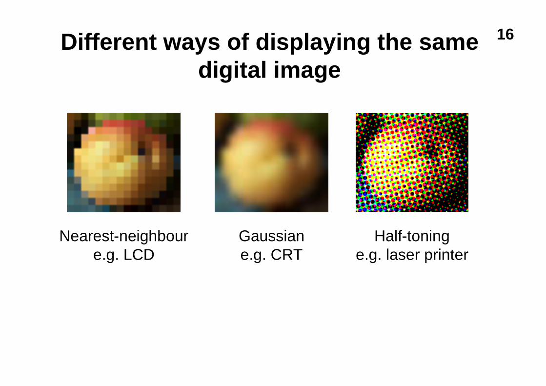
16Different ways of displaying the samedigital image

Nearest-neighboure.g. LCD

Gaussiane.g. CRT

Half-toninge.g. laser printer

17

Sampling

�a digital image is a rectangular array ofintensity values

�each value is called a pixelu “picture element”

�sampling resolution is normally measured inpixels per inch (ppi) or dots per inch (dpi)

n computer monitors have a resolution around 100 ppin laser printers have resolutions between 300 and 1200 ppi

18

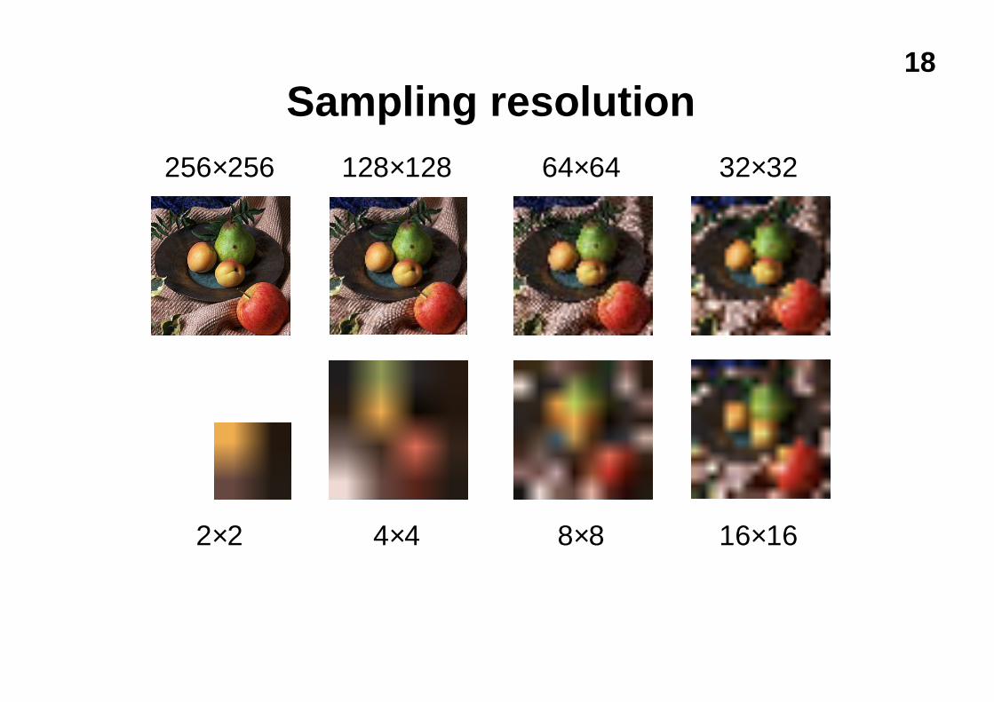
Sampling resolution256×256 128×128 64×64 32×32

2×2 4×4 8×8 16×16

19

Quantisation

�each intensity value is a number�for digital storage the intensity values must

be quantisedn limits the number of different intensities that can be

storedn limits the brightest intensity that can be stored

�how many intensity levels are needed forhuman consumption

n 8 bits usually sufficientn some applications use 10 or 12 bits

20

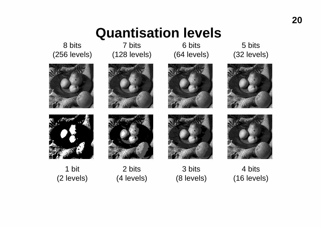
Quantisation levels8 bits

(256 levels)7 bits

(128 levels)6 bits

(64 levels)5 bits

(32 levels)

1 bit(2 levels)

2 bits(4 levels)

3 bits(8 levels)

4 bits(16 levels)

21

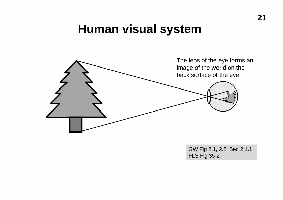
Human visual system

The lens of the eye forms animage of the world on theback surface of the eye

GW Fig 2.1, 2.2; Sec 2.1.1FLS Fig 35-2

22

Things eyes do

�discriminationn discriminates between different intensities and colours

�adaptationn adapts to changes in illumination level and colour

�simultaneous contrastn adapts locally within an image

�persistencen integrates light over a period of about 1/30 second

�edge enhancementn causes Mach banding effects

GLA Fig 1.17GW Fig 2.4

23

Simultaneous contrast

The centre square is the same intensity in all four cases

24

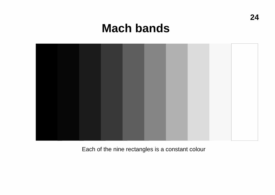
Mach bands

Each of the nine rectangles is a constant colour

25

Foveal vision

�150,000 cones per square millimetre in thefovea

n high resolutionn colour

�outside fovea: mostly rodsn lower resolutionn monochromatic

u peripheral visionl allows you to keep the high resolution region in context

l allows you to avoid being hit by passing branches

GW Fig 2.1, 2.2

26

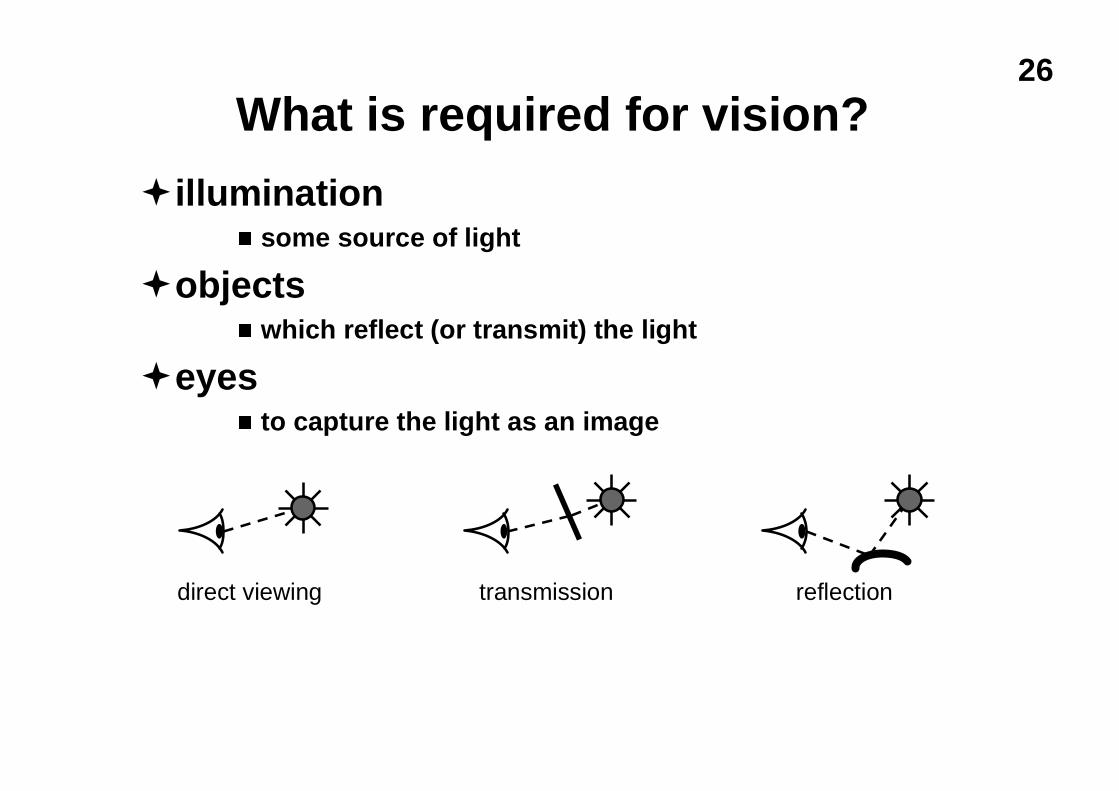
What is required for vision?

�illuminationn some source of light

�objectsn which reflect (or transmit) the light

�eyesn to capture the light as an image

direct viewing transmission reflection

27

Light: wavelengths & spectra

�light is electromagnetic radiationn visible light is a tiny part of the electromagnetic spectrumn visible light ranges in wavelength from 700nm (red end of

spectrum) to 400nm (violet end)

�every light has a spectrum of wavelengths thatit emits

�every object has a spectrum of wavelengthsthat it reflects (or transmits)

�the combination of the two gives the spectrumof wavelengths that arrive at the eye

MIN Fig 22a

MIN Examples 1 & 2

28

Classifying colours

�we want some way of classifying colours and,preferably, quantifying them

�we will discuss:u Munsell’s artists’ scheme

n which classifies colours on a perceptual basis

u the mechanism of colour visionn how colour perception works

u various colour spacesn which quantify colour based on either physical or

perceptual models of colour

29

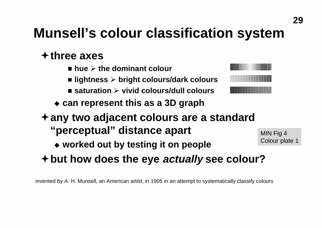
Munsell’s colour classification system

�three axesn hue À the dominant colourn lightness À bright colours/dark coloursn saturation À vivid colours/dull colours

u can represent this as a 3D graph

�any two adjacent colours are a standard“perceptual” distance apartu worked out by testing it on people

�but how does the eye actually see colour?

invented by A. H. Munsell, an American artist, in 1905 in an attempt to systematically classify colours

MIN Fig 4Colour plate 1

30

Colour vision

�three types of coneu each responds to a different spectrum

n roughly can be defined as red, green, and bluen each has a response function r(λ), g(λ), b(λ)

u different sensitivities to the different coloursn roughly 40:20:1n so cannot see fine detail in blue

u overall intensity response of the eye can becalculatedn y(λ) = r(λ) + g(λ) + b(λ)

n y = k ∫ P(λ) y(λ) dλ is the perceived luminance

JMF Fig 20b

31

Chromatic metamerismu many different spectra will induce the same response

in our conesn the values of the three perceived values can be calculated as:

l r = k ∫ P(λ) r(λ) dλl g = k ∫ P(λ) g(λ) dλl b = k ∫ P(λ) b(λ) dλ

n k is some constant, P(λ) is the spectrum of the light incident onthe retina

n two different spectra (e.g. P1(λ) and P2(λ)) can give the samevalues of r, g, b

n we can thus fool the eye into seeing (almost) any colour bymixing correct proportions of some small number of lights

32

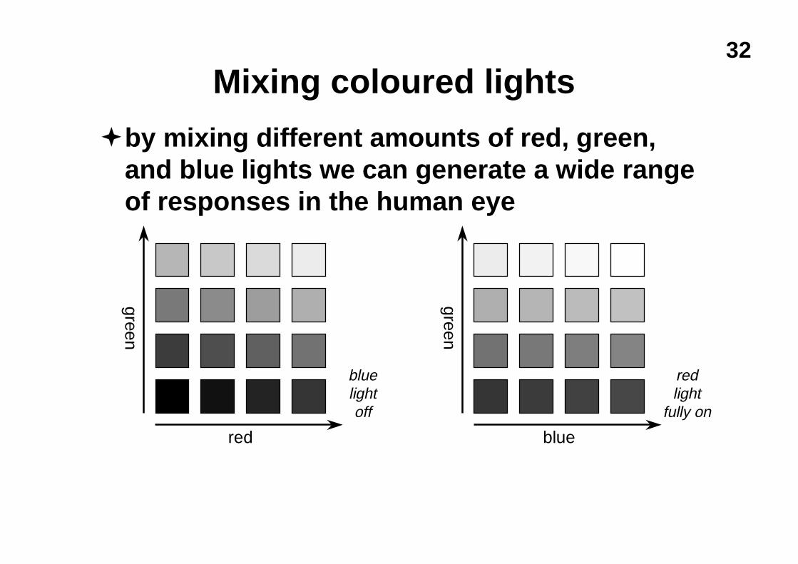
Mixing coloured lights

�by mixing different amounts of red, green,and blue lights we can generate a wide rangeof responses in the human eye

red

green

blue

green

bluelightoff

redlight

fully on

33

XYZ colour space

�not every wavelength can be represented as amix of red, green, and blue

�but matching & defining coloured light with amixture of three fixed primaries is desirable

�CIE define three standard primaries: X, Y, Zn Y matches the human eye’s response to light of a constant

intensity at each wavelength ( luminous-efficiency function of theeye)

n X, Y, and Z are not themselves colours, they are used fordefining colours – you cannot make a light that emits one ofthese primaries

XYZ colour space was defined in 1931 by the Commission Internationale de l’ Éclairage (CIE)

FvDFH Sec 13.2.2Figs 13.20, 13.22, 13.23

34

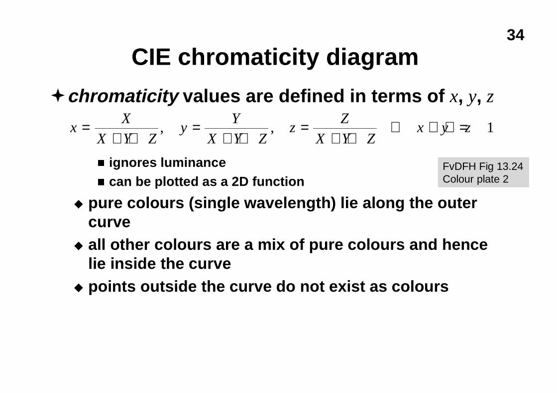
CIE chromaticity diagram

�chromaticity values are defined in terms of x, y, z

n ignores luminancen can be plotted as a 2D function

u pure colours (single wavelength) lie along the outercurve

u all other colours are a mix of pure colours and hencelie inside the curve

u points outside the curve do not exist as colours

xX

X Y Zy

Y

X Y Zz

Z

X Y Zx y z=

+ +=

+ +=

+ +∴ + + =, , 1

FvDFH Fig 13.24Colour plate 2

35

RGB in XYZ space

�CRTs and LCDs mix red, green, and blue tomake all other colours

�the red, green, and blue primaries each map toa point in XYZ space

�any colour within the resulting triangle can bedisplayed

n any colour outside the triangle cannot be displayedn for example: CRTs cannot display very saturated purples,

blues, or greens

FvDFH Figs 13.26, 13.27

36

Colour spacesu CIE XYZ, Yxy

u Pragmaticn used because they relate directly to the way that the hardware

worksn RGB, CMY, YIQ, YUV

u Munsell-liken considered by many to be easier for people to use than the

pragmatic colour spacesn HSV, HLS

u Uniformn equal steps in any direction make equal perceptual differencesn L*a*b*, L*u*v*

YIQ and YUV are usedin broadcast television

FvDFH Fig 13.28

FvDFH Figs 13.30, 13,35

GLA Figs 2.1, 2.2; Colour plates 3 & 4

37

Summary of colour spacesu the eye has three types of colour receptoru therefore we can validly use a three-dimensional

co-ordinate system to represent colouru XYZ is one such co-ordinate system

n Y is the eye’s response to intensity (luminance)n X and Z are, therefore, the colour co-ordinates

l same Y, change X or Z ⇒ same intensity, different colour

l same X and Z, change Y ⇒ same colour, different intensity

u some other systems use three colour co-ordinatesn luminance can then be derived as some function of the three

l e.g. in RGB: Y = 0.299 R + 0.587 G + 0.114 B

38

Implications of vision on resolutionu in theory you can see about 600dpi, 30cm from

your eyeu in practice, opticians say that the acuity of the eye

is measured as the ability to see a white gap,1 minute wide, between two black linesn about 300dpi at 30cm

u resolution decreases as contrast decreasesu colour resolution is much worse than intensity

resolutionn hence YIQ and YUV for TV broadcast

39

Implications of vision on quantisation�humans can distinguish, at best, about a 2%

change in intensityu not so good at distinguishing colour differences

�for TV ⇒ 10 bits of intensity informationu 8 bits is usually sufficient

l why use only 8 bits? why is it usually acceptable?

u for movie film ⇒ 14 bits of intensity information

for TV the brightest white is about 25x as bright asthe darkest black

movie film has about 10x the contrast ratio of TV

40

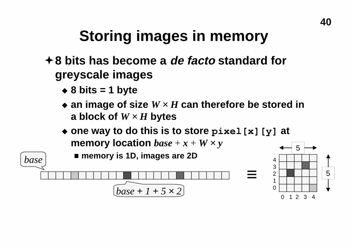
Storing images in memory

�8 bits has become a de facto standard forgreyscale imagesu 8 bits = 1 byteu an image of size W × H can therefore be stored in

a block of W × H bytesu one way to do this is to store pixel[x][y] at

memory location base + x + W × yn memory is 1D, images are 2Dbase

base + 1 + 5 × 2

5

5

43210

0 1 2 3 4

≡

41

Colour imagesu tend to be 24 bits per pixel

n 3 bytes: one red, one green, one blue

u can be stored as a contiguous block of memoryn of size W × H × 3

u more common to store each colour in a separate “plane”n each plane contains just W × H values

u the idea of planes can be extended to other attributesassociated with each pixeln alpha plane (transparency), z-buffer (depth value), A-buffer (pointer

to a data structure containing depth and coverage information),overlay planes (e.g. for displaying pop-up menus)

42

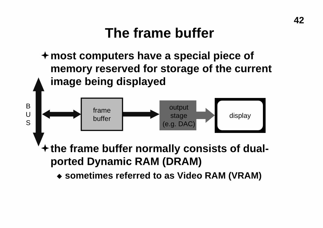
The frame buffer

�most computers have a special piece ofmemory reserved for storage of the currentimage being displayed

�the frame buffer normally consists of dual-ported Dynamic RAM (DRAM)u sometimes referred to as Video RAM (VRAM)

outputstage

(e.g. DAC)display

framebuffer

BUS

43

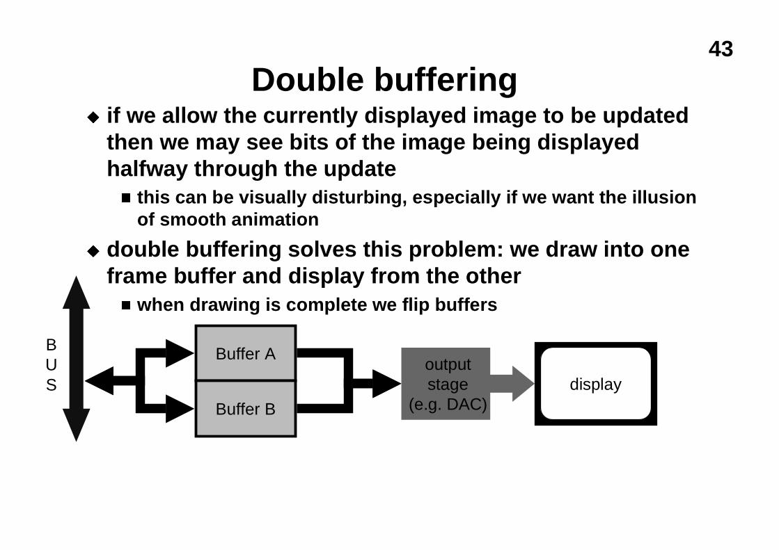
Double bufferingu if we allow the currently displayed image to be updated

then we may see bits of the image being displayedhalfway through the updaten this can be visually disturbing, especially if we want the illusion

of smooth animation

u double buffering solves this problem: we draw into oneframe buffer and display from the othern when drawing is complete we flip buffers

outputstage

(e.g. DAC)display

Buffer ABUS

Buffer B

44

Image display

�three technologies cover over 99% of alldisplay devicesu cathode ray tubeu liquid crystal displayu printer

45

Liquid crystal displayu liquid crystal can twist the polarisation of lightu control is by the voltage that is applied across the

liquid crystaln either on or off: transparent or opaque

u greyscale can be achieved in some liquid crystalsby varying the voltage

u colour is achieved with colour filtersu low power consumption but image quality not as

good as cathode ray tubes

JMF Figs 90, 91

46

Cathode ray tubesu focus an electron gun on a phosphor screen

n produces a bright spot

u scan the spot back and forth, up and down tocover the whole screen

u vary the intensity of the electron beam to changethe intensity of the spot

u repeat this fast enough and humans see acontinuous picture

CRT slides in handout

47

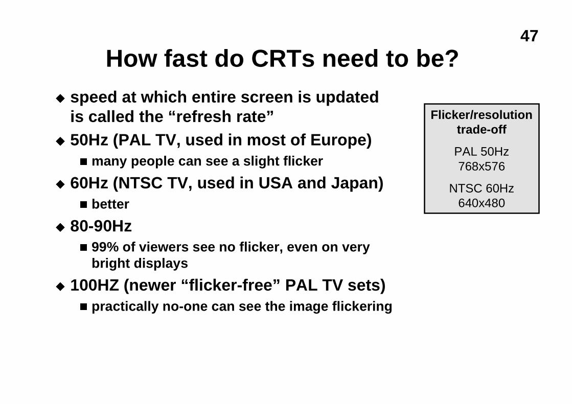
How fast do CRTs need to be?u speed at which entire screen is updated

is called the “refresh rate”u 50Hz (PAL TV, used in most of Europe)

n many people can see a slight flicker

u 60Hz (NTSC TV, used in USA and Japan)n better

u 80-90Hzn 99% of viewers see no flicker, even on very

bright displays

u 100HZ (newer “flicker-free” PAL TV sets)n practically no-one can see the image flickering

Flicker/resolutiontrade-off

PAL 50Hz768x576

NTSC 60Hz640x480

48

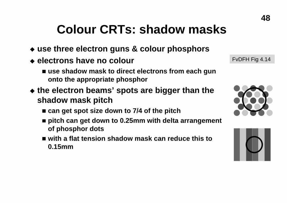
Colour CRTs: shadow masksu use three electron guns & colour phosphorsu electrons have no colour

n use shadow mask to direct electrons from each gunonto the appropriate phosphor

u the electron beams’ spots are bigger than theshadow mask pitchn can get spot size down to 7/4 of the pitchn pitch can get down to 0.25mm with delta arrangement

of phosphor dotsn with a flat tension shadow mask can reduce this to

0.15mm

FvDFH Fig 4.14

49

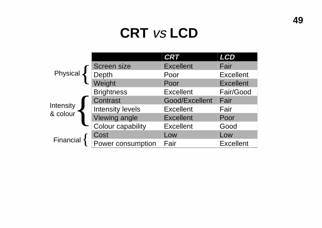
CRT vs LCD

CRT LCDScreen size Excellent FairDepth Poor ExcellentWeight Poor ExcellentBrightness Excellent Fair/GoodContrast Good/Excellent FairIntensity levels Excellent FairViewing angle Excellent PoorColour capability Excellent GoodCost Low LowPower consumption Fair Excellent

Physical

Intensity& colour

Financial

{

{{

50

Printers

�many types of printeru ink jet

n sprays ink onto paper

u dot matrixn pushes pins against an ink ribbon and onto the paper

u laser printern uses a laser to lay down a pattern of charge on a drum;

this picks up charged toner which is then pressed ontothe paper

�all make marks on paperu essentially binary devices: mark/no mark

51

Printer resolution

�ink jetu up to 360dpi

�laser printeru up to 1200dpiu generally 600dpi

�phototypesetteru up to about 3000dpi

�bi-level devices: each pixel is either black orwhite

52

What about greyscale?u achieved by halftoning

n divide image into cells, in each cell draw a spot of theappropriate size for the intensity of that cell

n on a printer each cell is m×m pixels, allowing m2+1 differentintensity levels

n e.g. 300dpi with 4×4 cells ⇒ 75 cells per inch, 17 intensitylevels

n phototypesetters can make 256 intensity levels in cells sosmall you can only just see them

u an alternative method is ditheringn dithering photocopies badly, halftoning photocopies well

will discuss halftoning and dithering in Image Processing section of course

53

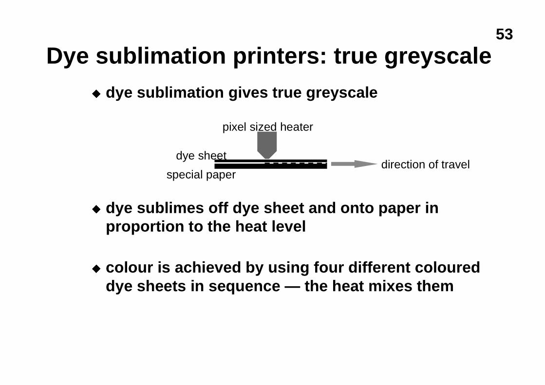
Dye sublimation printers: true greyscaleu dye sublimation gives true greyscale

u dye sublimes off dye sheet and onto paper inproportion to the heat level

u colour is achieved by using four different coloureddye sheets in sequence — the heat mixes them

pixel sized heater

dye sheet

special paperdirection of travel

54

What about colour?�generally use cyan, magenta, yellow, and black

inks (CMYK)�inks aborb colour

u c.f. lights which emit colouru CMY is the inverse of RGB

�why is black (K) necessary?u inks are not perfect aborbersu mixing C + M + Y gives a muddy grey, not blacku lots of text is printed in black: trying to align C, M

and Y perfectly for black text would be a nightmare

JMF Fig 9b

55

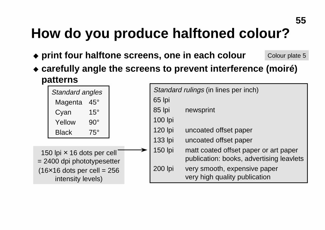
How do you produce halftoned colour?u print four halftone screens, one in each colouru carefully angle the screens to prevent interference (moiré)

patternsStandard angles Magenta 45° Cyan 15° Yellow 90°

Black 75°

Standard rulings (in lines per inch)65 lpi85 lpi newsprint100 lpi

120 lpi uncoated offset paper133 lpi uncoated offset paper150 lpi matt coated offset paper or art paper

publication: books, advertising leavlets200 lpi very smooth, expensive paper

very high quality publication

150 lpi × 16 dots per cell= 2400 dpi phototypesetter(16×16 dots per cell = 256

intensity levels)

Colour plate 5

56

2D Computer Graphics�lines

n how do I draw a straight line?

�curvesn how do I specify curved lines?

�clippingn what about lines that go off the edge of the screen?

�filled areas�transformations

n scaling, rotation, translation, shearing

�applications

IP

3D CG

Background

2D CG

57

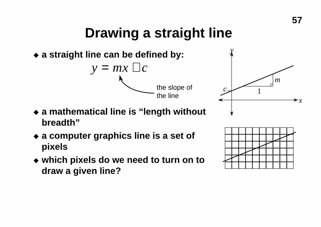
Drawing a straight lineu a straight line can be defined by:

u a mathematical line is “length withoutbreadth”

u a computer graphics line is a set ofpixels

u which pixels do we need to turn on todraw a given line?

y mx c= +the slope ofthe line

x

y

m

1c

58

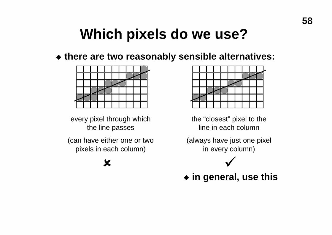
Which pixels do we use?u there are two reasonably sensible alternatives:

every pixel through whichthe line passes

(can have either one or twopixels in each column)

the “closest” pixel to theline in each column

(always have just one pixelin every column)

u in general, use thisäã

59

A line drawing algorithm - preparation 1

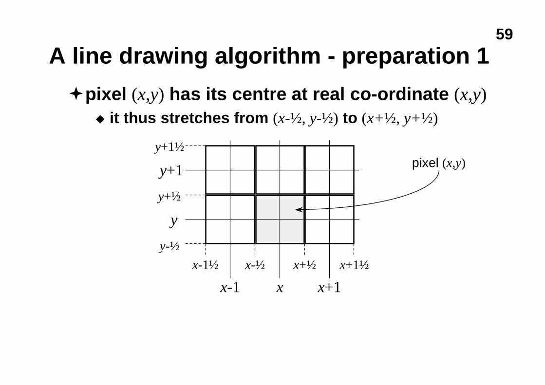
�pixel (x,y) has its centre at real co-ordinate (x,y)u it thus stretches from (x-½, y-½) to (x+½, y+½)

y

x-1 x+1x

y+1

x-½

y-½

y+½

y+1½

x+½ x+1½x-1½

pixel (x,y)

60

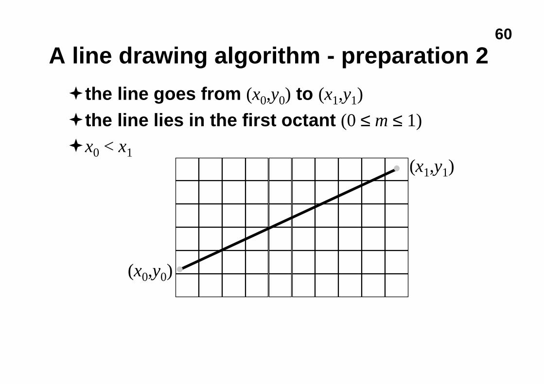
A line drawing algorithm - preparation 2

�the line goes from (x0,y0) to (x1,y1)

�the line lies in the first octant (0 ≤ m ≤ 1)

�x0 < x1

(x0,y0)

(x1,y1)

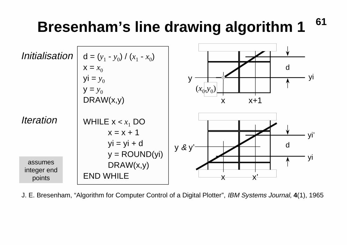
61Bresenham’s line drawing algorithm 1

Initialisation d = (y1 - y0) / (x1 - x0)x = x0

yi = y0

y = y0

DRAW(x,y)

WHILE x < x1 DOx = x + 1yi = yi + dy = ROUND(yi)DRAW(x,y)

END WHILE

y

x x+1

dyi

(x0,y0)

y & y’

x x’

d

yi

yi’

Iteration

J. E. Bresenham, “Algorithm for Computer Control of a Digital Plotter”, IBM Systems Journal, 4(1), 1965

assumesinteger end

points

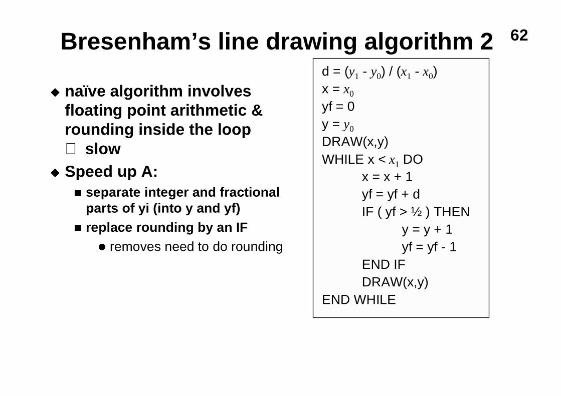
62Bresenham’s line drawing algorithm 2

u naïve algorithm involvesfloating point arithmetic &rounding inside the loop⇒ slow

u Speed up A:n separate integer and fractional

parts of yi (into y and yf)n replace rounding by an IF

l removes need to do rounding

d = (y1 - y0) / (x1 - x0)x = x0

yf = 0y = y0

DRAW(x,y)WHILE x < x1 DO

x = x + 1yf = yf + dIF ( yf > ½ ) THEN

y = y + 1yf = yf - 1

END IFDRAW(x,y)

END WHILE

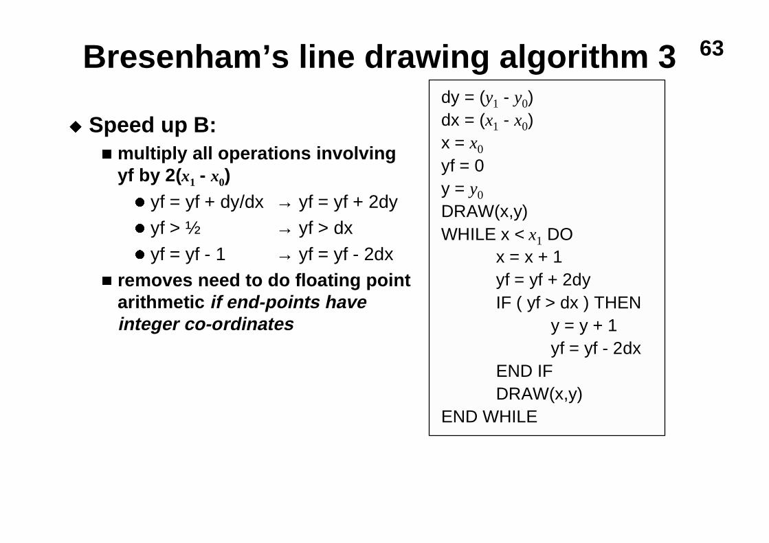
63Bresenham’s line drawing algorithm 3

u Speed up B:n multiply all operations involving

yf by 2(x1 - x0)l yf = yf + dy/dx → yf = yf + 2dyl yf > ½ → yf > dx

l yf = yf - 1 → yf = yf - 2dxn removes need to do floating point

arithmetic if end-points haveinteger co-ordinates

dy = (y1 - y0)dx = (x1 - x0)x = x0

yf = 0y = y0

DRAW(x,y)WHILE x < x1 DO

x = x + 1yf = yf + 2dyIF ( yf > dx ) THEN

y = y + 1yf = yf - 2dx

END IFDRAW(x,y)

END WHILE

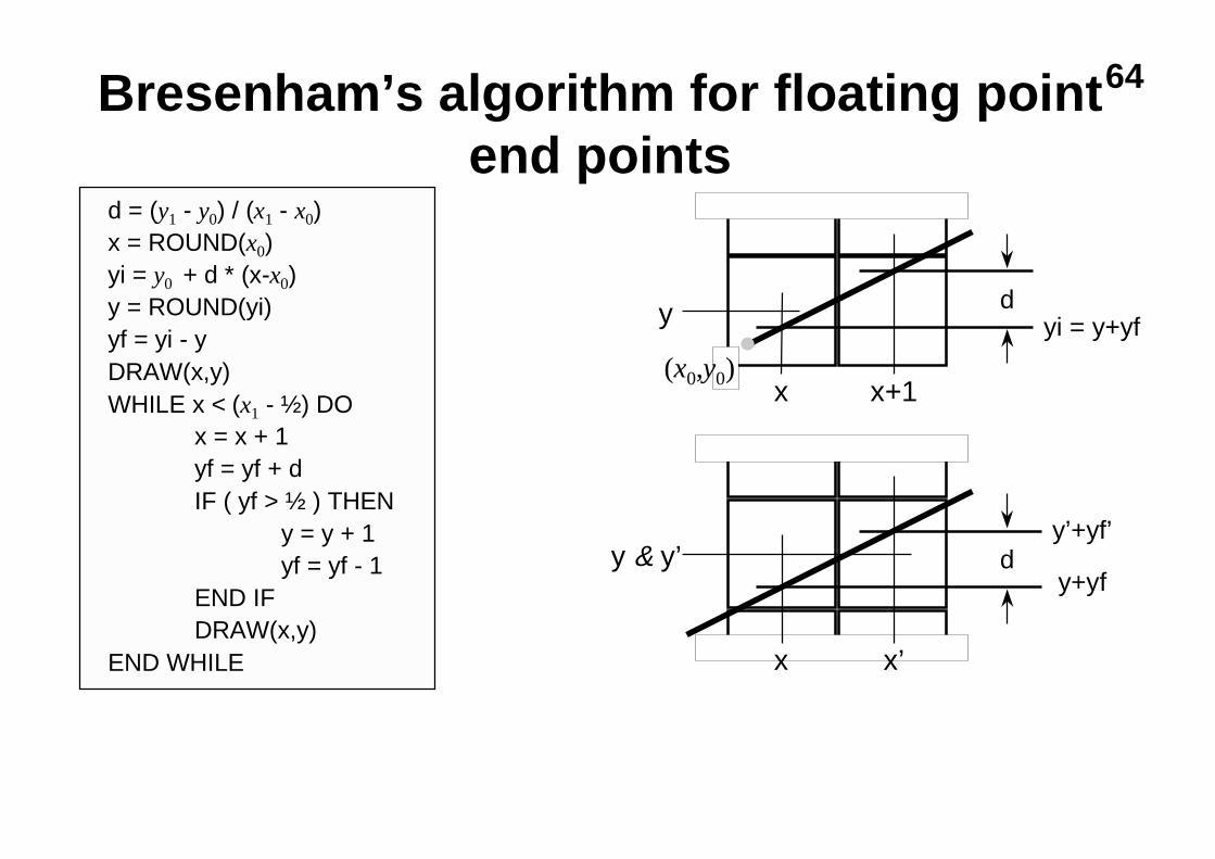
64Bresenham’s algorithm for floating pointend points

y

x x+1

dyi = y+yf

(x0,y0)

y & y’

x x’

dy’+yf’

d = (y1 - y0) / (x1 - x0)x = ROUND(x0)yi = y0 + d * (x-x0)y = ROUND(yi)yf = yi - yDRAW(x,y)WHILE x < (x1 - ½) DO

x = x + 1yf = yf + dIF ( yf > ½ ) THEN

y = y + 1yf = yf - 1

END IFDRAW(x,y)

END WHILE

y+yf

65

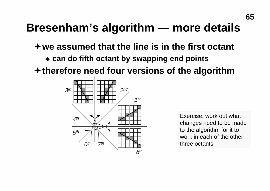
Bresenham’s algorithm — more details

�we assumed that the line is in the first octantu can do fifth octant by swapping end points

�therefore need four versions of the algorithm

1st

2nd3rd

4th

5th

6th 7th

8th

Exercise: work out whatchanges need to be madeto the algorithm for it towork in each of the otherthree octants

66

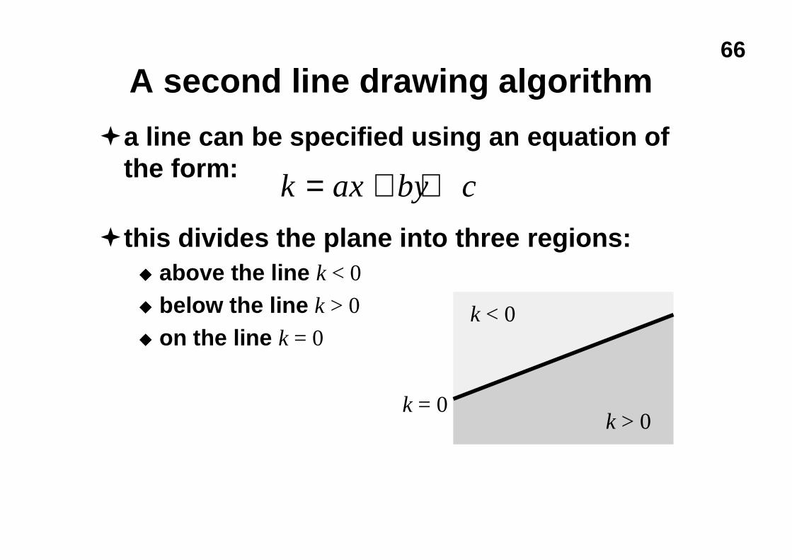
A second line drawing algorithm

�a line can be specified using an equation ofthe form:

�this divides the plane into three regions:u above the line k < 0

u below the line k > 0

u on the line k = 0

k ax by c= + +

k < 0

k > 0k = 0

67

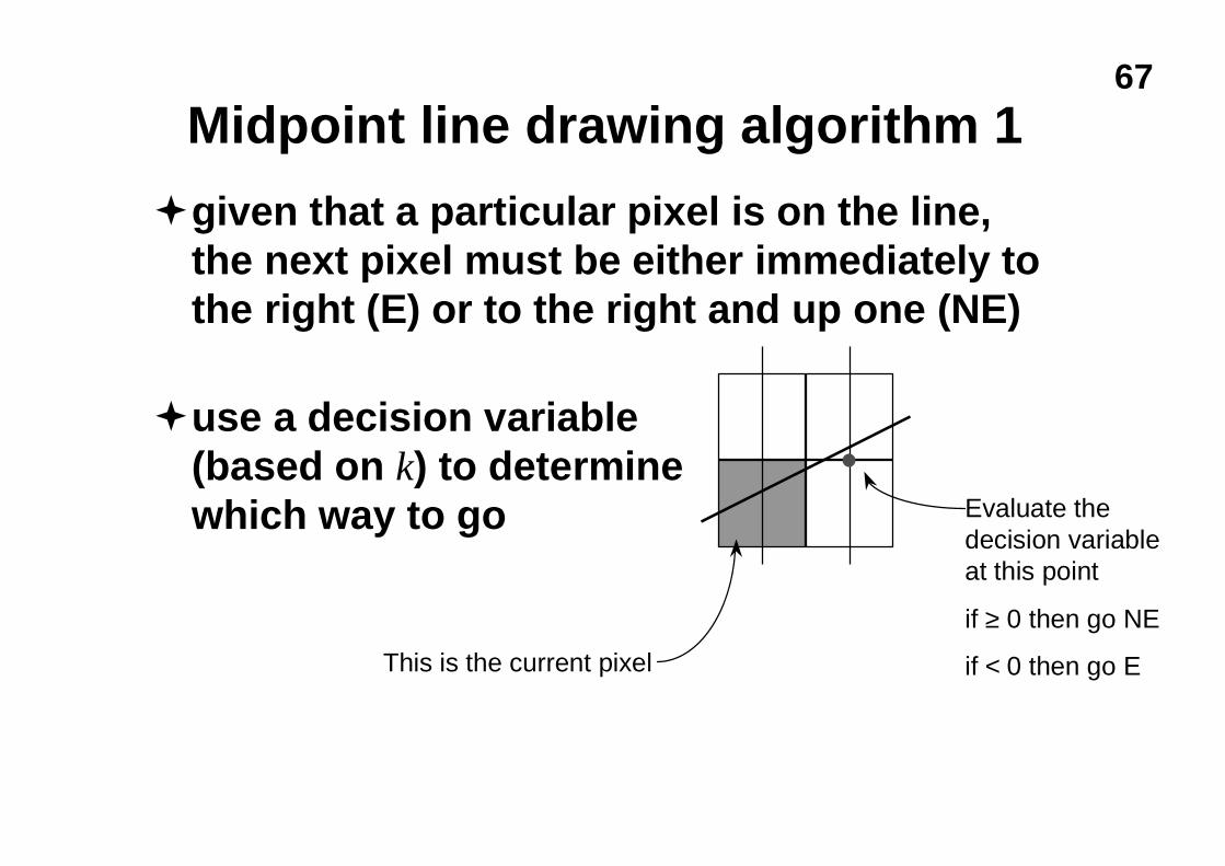
Midpoint line drawing algorithm 1

�given that a particular pixel is on the line,the next pixel must be either immediately tothe right (E) or to the right and up one (NE)

�use a decision variable(based on k) to determinewhich way to go Evaluate the

decision variableat this point

if ≥ 0 then go NE

if < 0 then go EThis is the current pixel

68

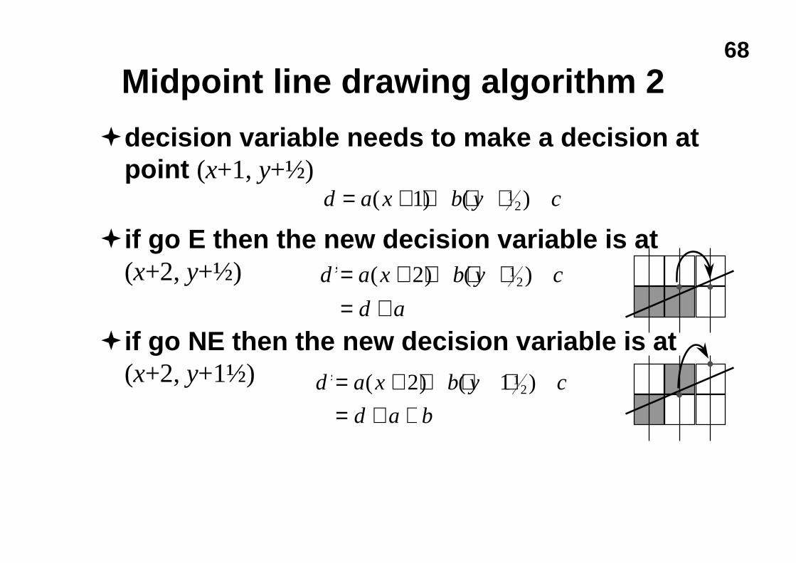
Midpoint line drawing algorithm 2

�decision variable needs to make a decision atpoint (x+1, y+½)

�if go E then the new decision variable is at(x+2, y+½)

�if go NE then the new decision variable is at(x+2, y+1½)

d a x b y c= + + + +( ) ( )1 12

d a x b y c

d a

’ ( ) ( )= + + + += +

2 12

d a x b y c

d a b

’ ( ) ( )= + + + += + +

2 1 12

69

Midpoint line drawing algorithm 3

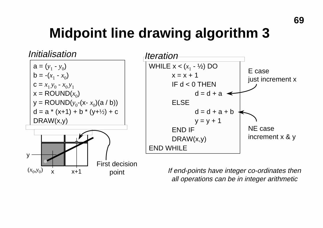
a = (y1 - y0)b = -(x1 - x0)c = x1 y0 - x0 y1

x = ROUND(x0)y = ROUND(y0-(x- x0)(a / b))d = a * (x+1) + b * (y+½) + cDRAW(x,y)

WHILE x < (x1 - ½) DOx = x + 1IF d < 0 THEN

d = d + aELSE

d = d + a + by = y + 1

END IFDRAW(x,y)

END WHILE

Initialisation Iteration

y

x x+1(x0,y0)First decision

point

E casejust increment x

NE caseincrement x & y

If end-points have integer co-ordinates thenall operations can be in integer arithmetic

70

Midpoint - comments

�this version only works for lines in the firstoctantu extend to other octants as for Bresenham

�Sproull has proven that Bresenham andMidpoint give identical results

�Midpoint algorithm can be generalised todraw arbitary circles & ellipsesu Bresenham can only be generalised to draw

circles with integer radii

71

Curves

�circles & ellipses�Bezier cubics

n Pierre Bézier, worked in CAD for Citroënn widely used in Graphic Design

�Overhauser cubicsn Overhauser, worked in CAD for Ford

�NURBSn Non-Uniform Rational B-Splinesn more powerful than Bezier & now more widely usedn consider these next year

72

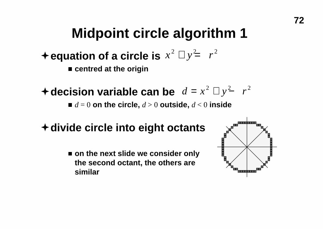
Midpoint circle algorithm 1

�equation of a circle isn centred at the origin

�decision variable can ben d = 0 on the circle, d > 0 outside, d < 0 inside

�divide circle into eight octants

n on the next slide we consider onlythe second octant, the others aresimilar

x y r2 2 2+ =

d x y r= + −2 2 2

73

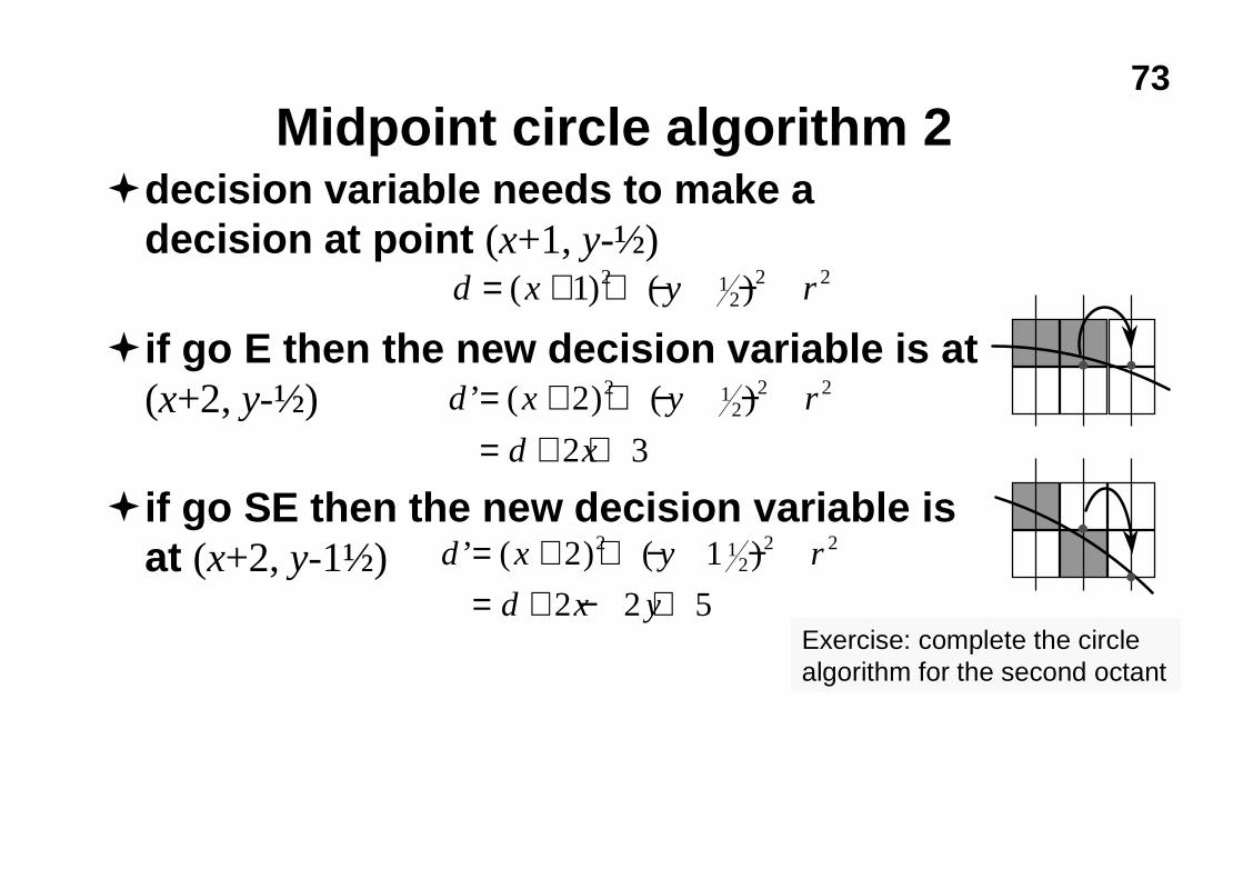
Midpoint circle algorithm 2�decision variable needs to make a

decision at point (x+1, y-½)

�if go E then the new decision variable is at(x+2, y-½)

�if go SE then the new decision variable isat (x+2, y-1½)

d x y r= + + − −( ) ( )1 2 12

2 2

d x y r

d x

’ ( ) ( )= + + − −= + +

2

2 3

2 12

2 2

d x y r

d x y

’ ( ) ( )= + + − −= + − +

2 1

2 2 5

2 12

2 2

Exercise: complete the circlealgorithm for the second octant

74

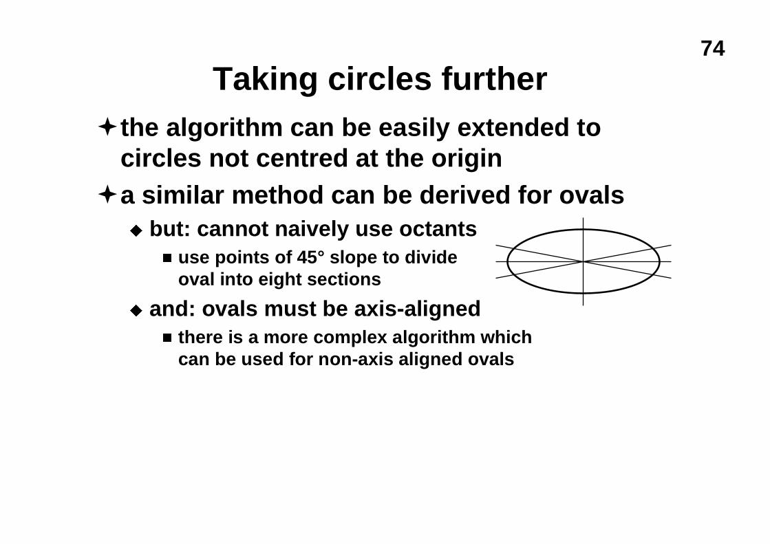
Taking circles further�the algorithm can be easily extended to

circles not centred at the origin�a similar method can be derived for ovals

u but: cannot naively use octantsn use points of 45° slope to divide

oval into eight sections

u and: ovals must be axis-alignedn there is a more complex algorithm which

can be used for non-axis aligned ovals

75

Are circles & ellipses enough?

�simple drawing packages use ellipses &segments of ellipses

�for graphic design & CAD need somethingwith more flexibilityu use cubic polynomials

76

Why cubics?

�lower orders cannot:u have a point of inflectionu match both position and slope at both ends of a

segmentu be non-planar in 3D

�higher orders:u can wiggle too muchu take longer to compute

77

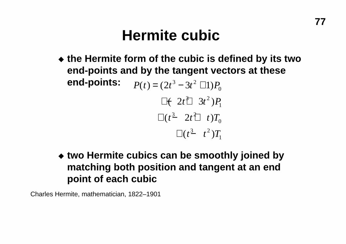
Hermite cubicu the Hermite form of the cubic is defined by its two

end-points and by the tangent vectors at theseend-points:

u two Hermite cubics can be smoothly joined bymatching both position and tangent at an endpoint of each cubic

P t t t P

t t P

t t t T

t t T

( ) ( )

( )

( )

( )

= − +

+ − +

+ − +

+ −

2 3 1

2 3

2

3 20

3 21

3 20

3 21

Charles Hermite, mathematician, 1822–1901

78

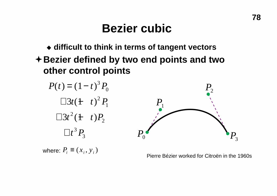
Bezier cubicu difficult to think in terms of tangent vectors

�Bezier defined by two end points and twoother control points

P t t P

t t P

t t P

t P

( ) ( )

( )

( )

= −

+ −

+ −

+

1

3 1

3 1

30

21

22

33 P0

P1

P2

P3

Pierre Bézier worked for Citroën in the 1960swhere: P x yi i i≡ ( , )

79

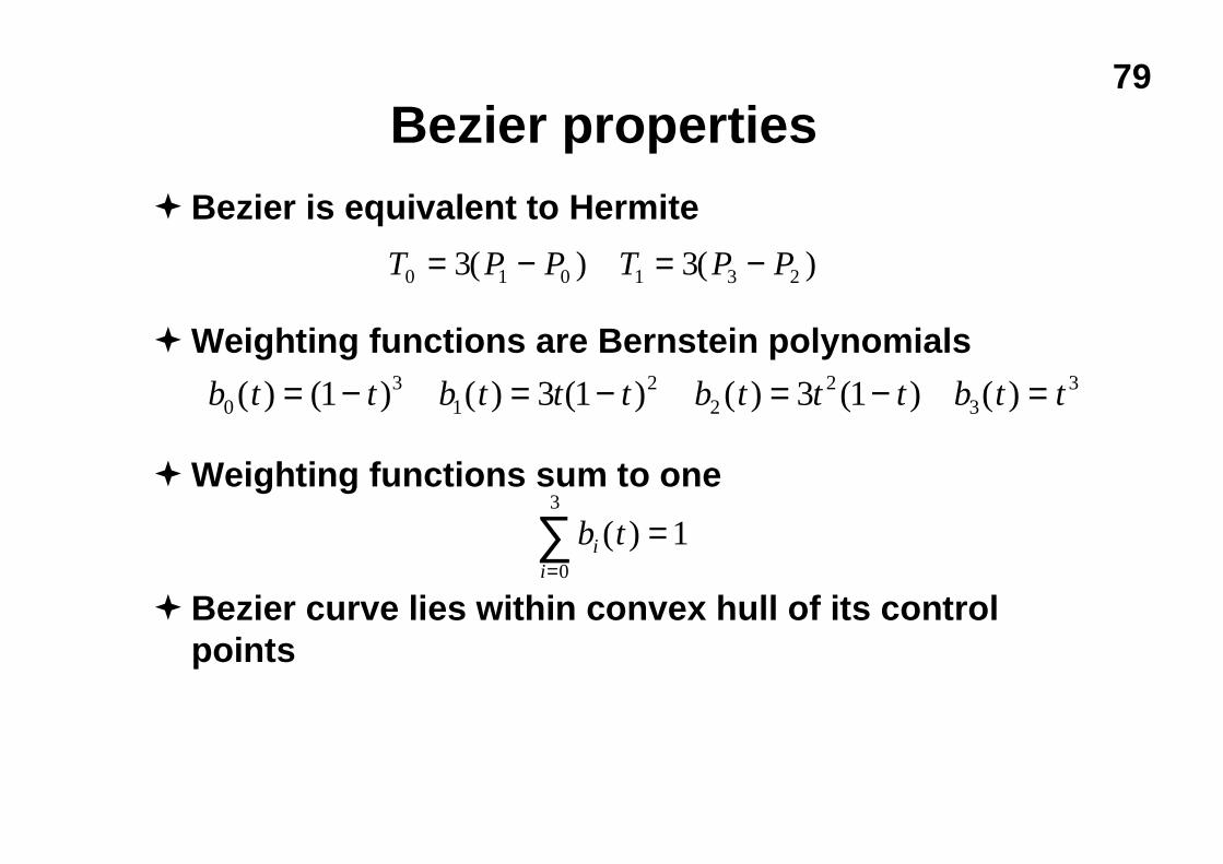
Bezier properties�Bezier is equivalent to Hermite

�Weighting functions are Bernstein polynomials

�Weighting functions sum to one

�Bezier curve lies within convex hull of its controlpoints

T P P T P P0 1 0 1 3 23 3= − = −( ) ( )

b t t b t t t b t t t b t t03

12

22

331 3 1 3 1( ) ( ) ( ) ( ) ( ) ( ) ( )= − = − = − =

b tii=∑ =

0

3

1( )

80

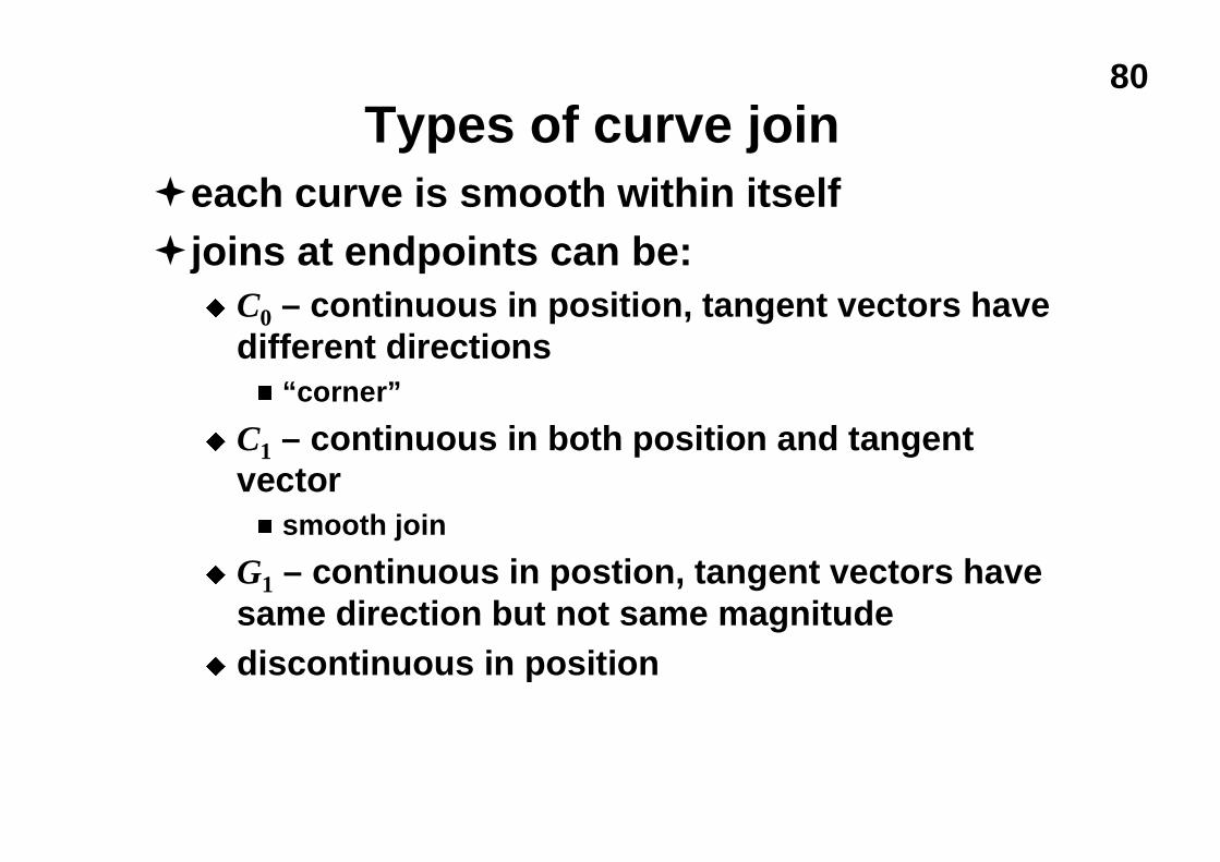
Types of curve join�each curve is smooth within itself�joins at endpoints can be:

u C0 – continuous in position, tangent vectors havedifferent directionsn “corner”

u C1 – continuous in both position and tangentvectorn smooth join

u G1 – continuous in postion, tangent vectors havesame direction but not same magnitude

u discontinuous in position

81

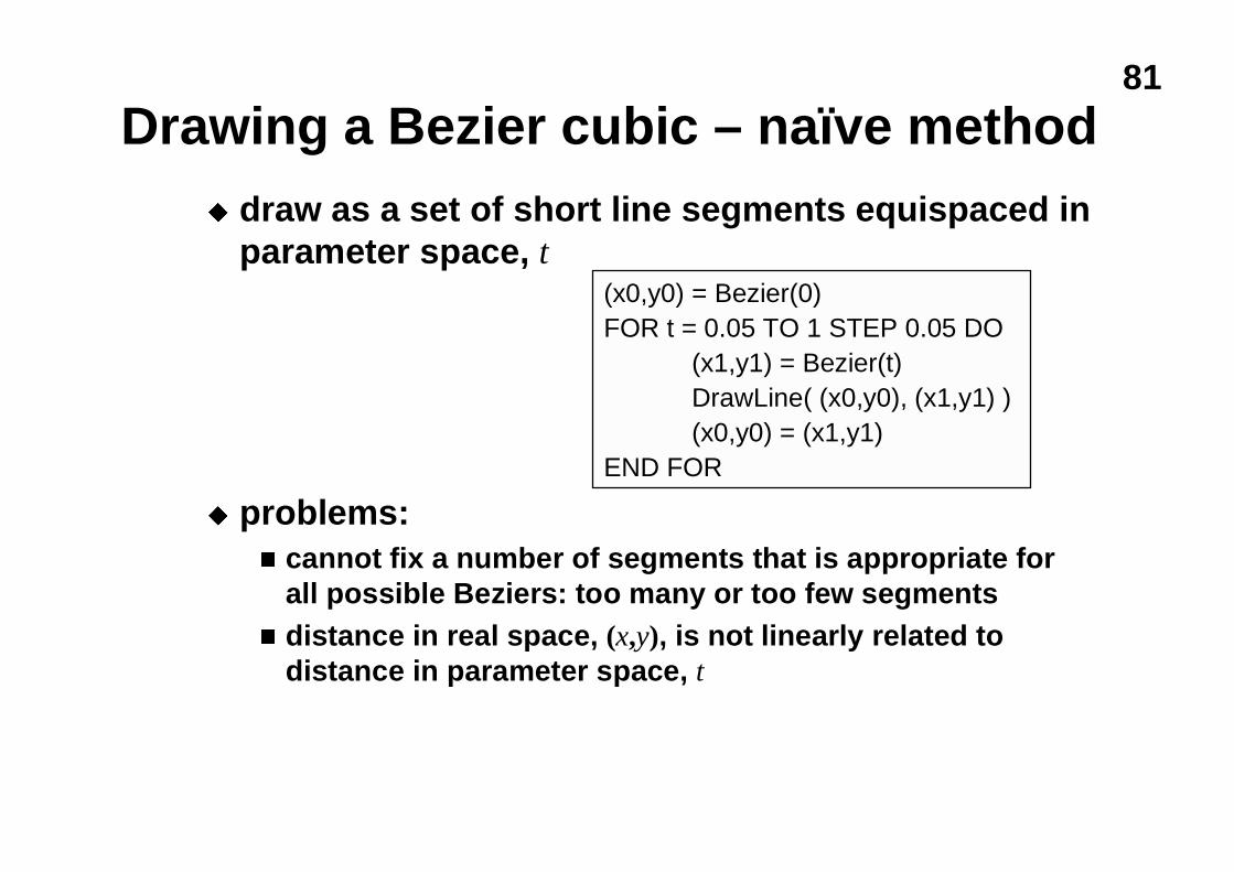
Drawing a Bezier cubic – naïve methodu draw as a set of short line segments equispaced in

parameter space, t

u problems:n cannot fix a number of segments that is appropriate for

all possible Beziers: too many or too few segmentsn distance in real space, (x,y), is not linearly related to

distance in parameter space, t

(x0,y0) = Bezier(0)FOR t = 0.05 TO 1 STEP 0.05 DO

(x1,y1) = Bezier(t)DrawLine( (x0,y0), (x1,y1) )(x0,y0) = (x1,y1)

END FOR

82

Drawing a Bezier cubic – sensible method

�adaptive subdivisionu check if a straight line between P0 and P3 is an

adequate approximation to the Bezieru if so: draw the straight lineu if not: divide the Bezier into two halves, each a

Bezier, and repeat for the two new Beziers

�need to specify some tolerance for when astraight line is an adequate approximationu when the Bezier lies within half a pixel width of the

straight line along its entire length

83

Drawing a Bezier cubic (continued)

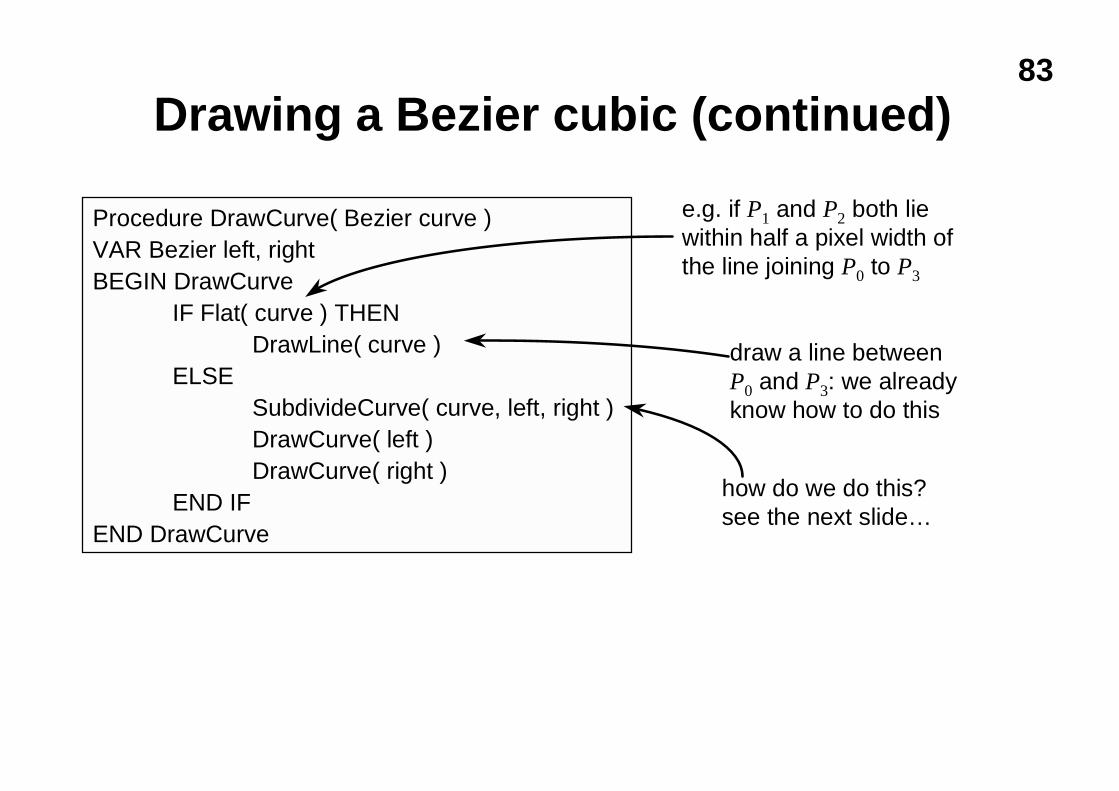
Procedure DrawCurve( Bezier curve )VAR Bezier left, rightBEGIN DrawCurve

IF Flat( curve ) THENDrawLine( curve )

ELSESubdivideCurve( curve, left, right )DrawCurve( left )DrawCurve( right )

END IFEND DrawCurve

e.g. if P1 and P2 both liewithin half a pixel width ofthe line joining P0 to P3

draw a line betweenP0 and P3: we alreadyknow how to do this

how do we do this?see the next slide…

84

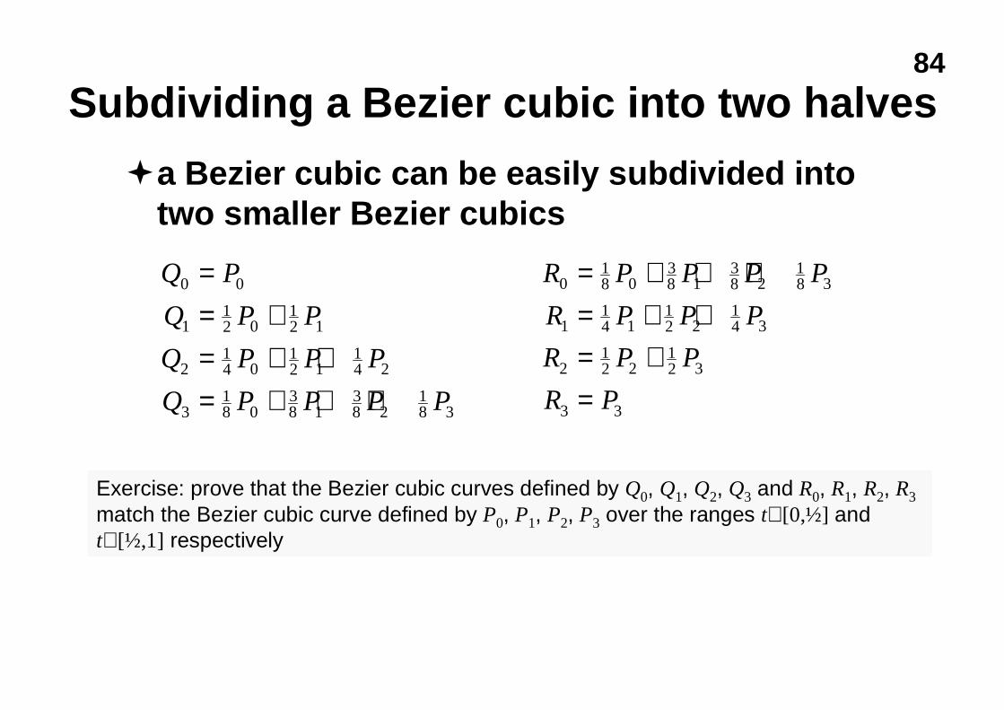
Subdividing a Bezier cubic into two halves

�a Bezier cubic can be easily subdivided intotwo smaller Bezier cubics

Q P

Q P P

Q P P P

Q P P P P

0 0

112 0

12 1

214 0

12 1

14 2

318 0

38 1

38 2

18 3

== += + += + + +

R P P P P

R P P P

R P P

R P

018 0

38 1

38 2

18 3

114 1

12 2

14 3

212 2

12 3

3 3

= + + += + += +=

Exercise: prove that the Bezier cubic curves defined by Q0, Q1, Q2, Q3 and R0, R1, R2, R3

match the Bezier cubic curve defined by P0, P1, P2, P3 over the ranges t∈[0,½] andt∈[½,1] respectively

85

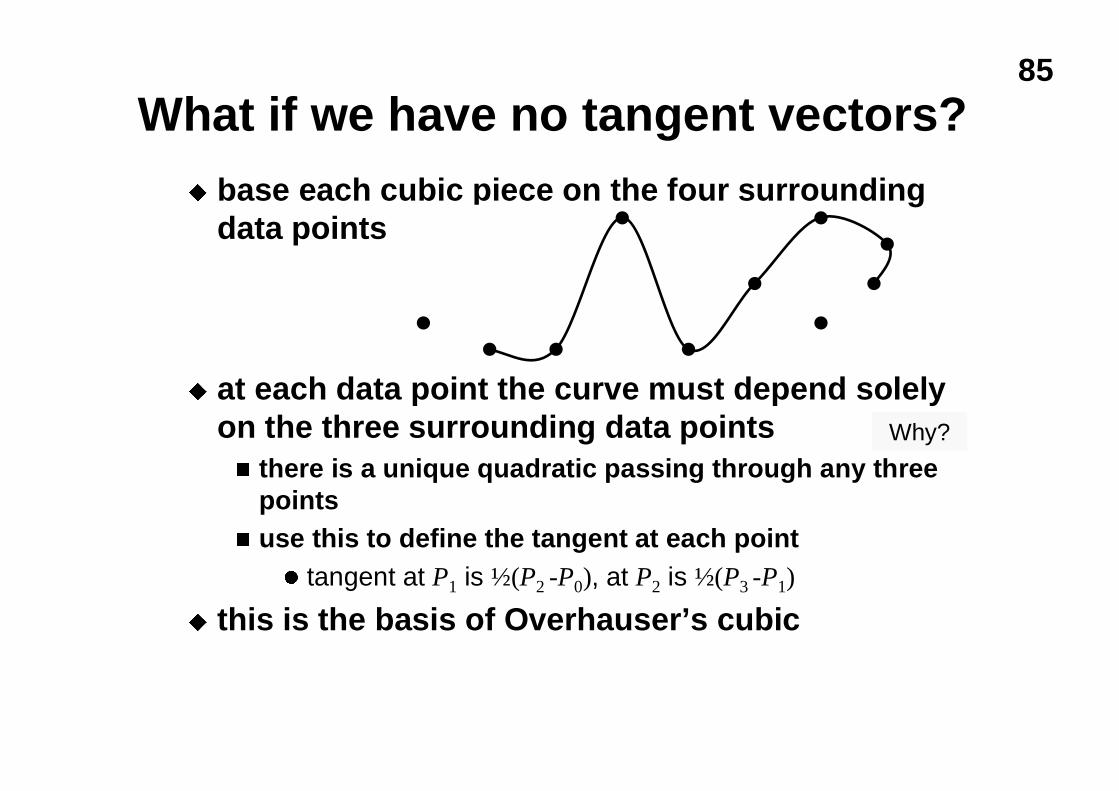
What if we have no tangent vectors?u base each cubic piece on the four surrounding

data points

u at each data point the curve must depend solelyon the three surrounding data pointsn there is a unique quadratic passing through any three

pointsn use this to define the tangent at each point

l tangent at P1 is ½(P2 -P0), at P2 is ½(P3 -P1)

u this is the basis of Overhauser’s cubic

Why?

86

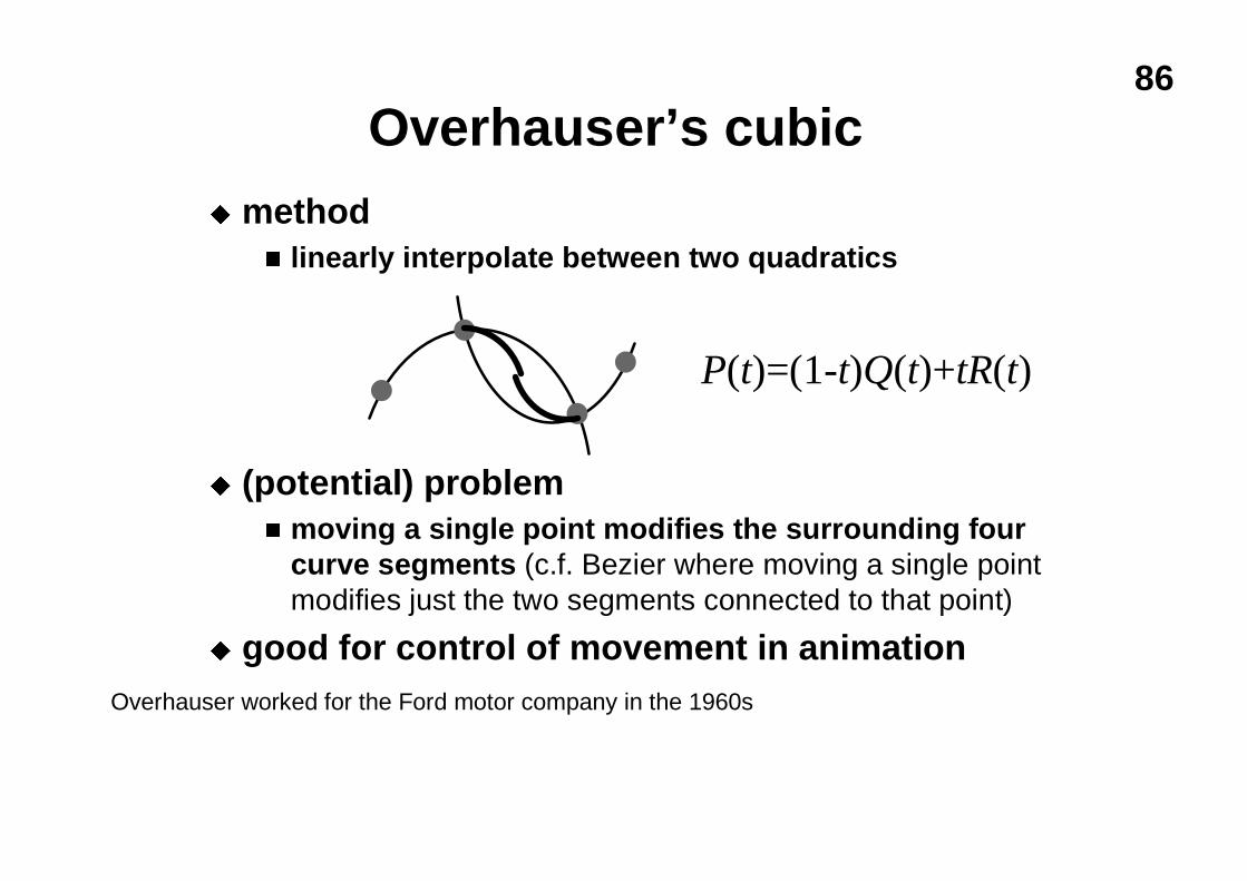
Overhauser’s cubicu method

n linearly interpolate between two quadratics

u (potential) problemn moving a single point modifies the surrounding four

curve segments (c.f. Bezier where moving a single pointmodifies just the two segments connected to that point)

u good for control of movement in animationOverhauser worked for the Ford motor company in the 1960s

P(t)=(1-t)Q(t)+tR(t)

87

Simplifying line chainsu the problem: you are given a chain of line segments

at a very high resolution, how can you reduce thenumber of line segments without compromising thequality of the linen e.g. given the coastline of Britain defined as a chain of line

segments at 10m resolution, draw the entire outline on a1280×1024 pixel screen

u the solution: Douglas & Pücker’s line chainsimplification algorithm

This can also be applied to chains of Bezier curves at high resolution: most of the curveswill each be approximated (by the previous algorithm) as a single line segment, Douglas& Pücker’s algorithm can then be used to further simplify the line chain

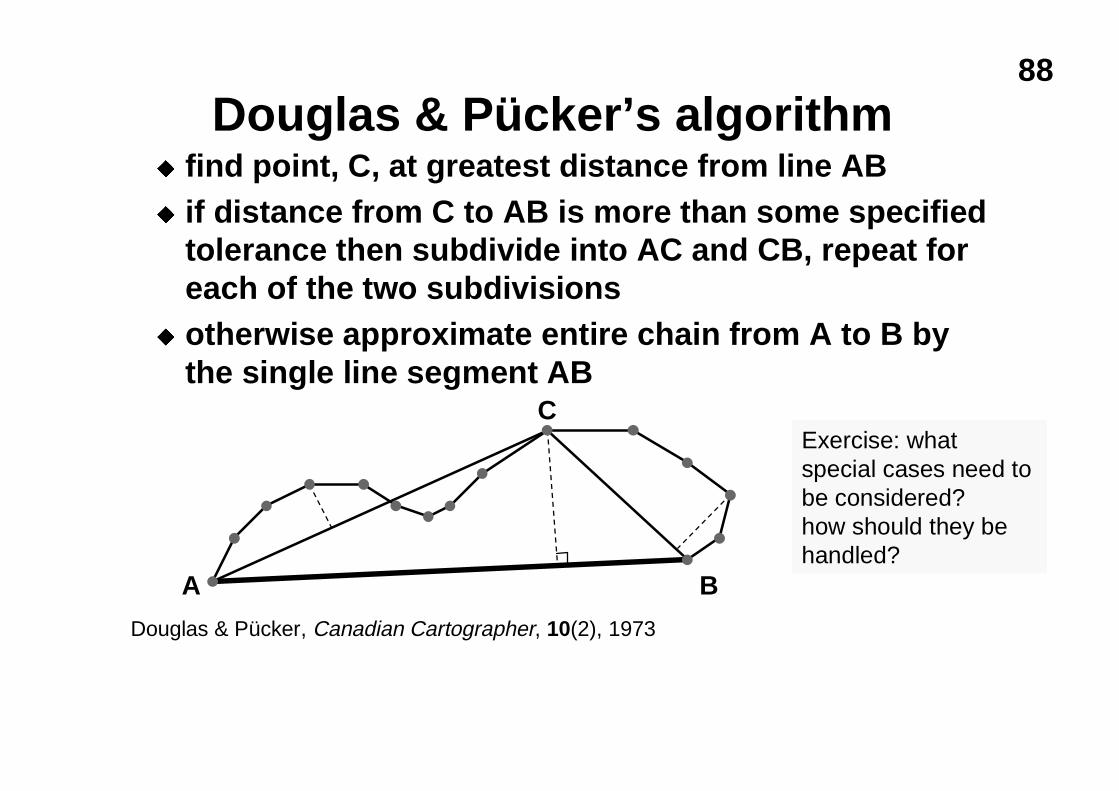
88

Douglas & Pücker’s algorithmu find point, C, at greatest distance from line ABu if distance from C to AB is more than some specified

tolerance then subdivide into AC and CB, repeat foreach of the two subdivisions

u otherwise approximate entire chain from A to B bythe single line segment AB

A B

CExercise: whatspecial cases need tobe considered?how should they behandled?

Douglas & Pücker, Canadian Cartographer, 10(2), 1973

89

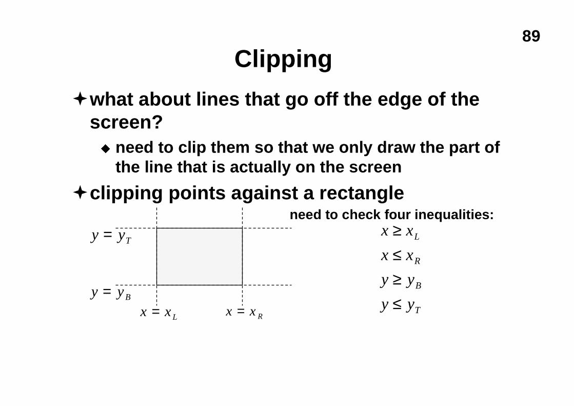
Clipping

�what about lines that go off the edge of thescreen?u need to clip them so that we only draw the part of

the line that is actually on the screen

�clipping points against a rectangle

y yT=

y yB=x x L= x x R=

need to check four inequalities:x x

x x

y y

y y

L

R

B

T

≥≤≥≤

90

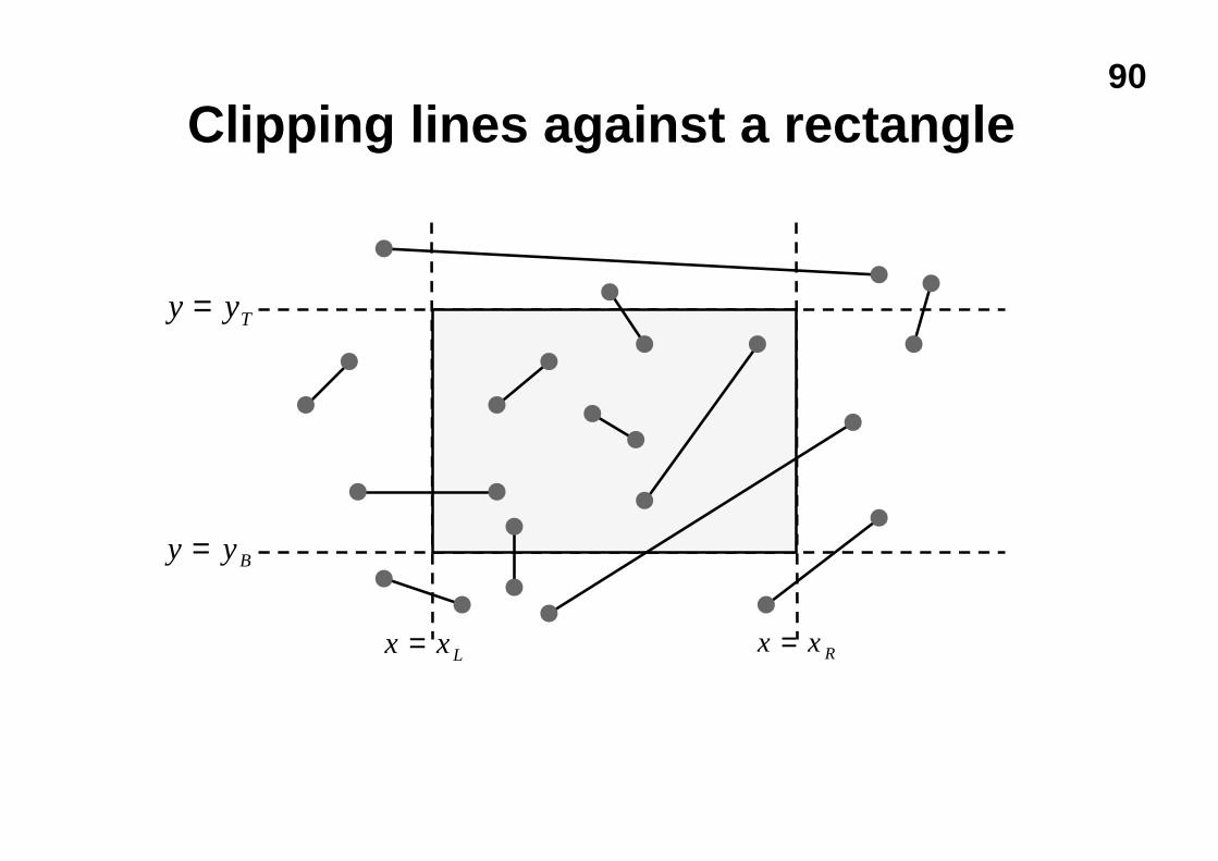
Clipping lines against a rectangle

y yT=

y yB=

x x L= x x R=

91

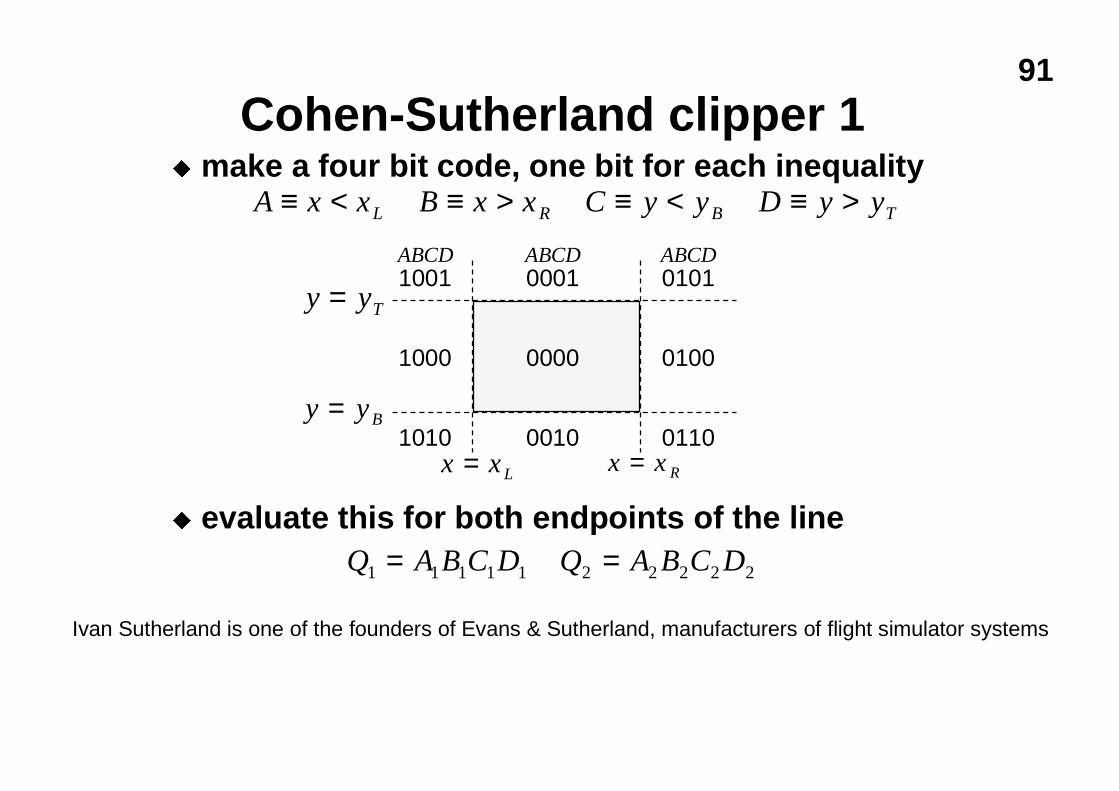
Cohen-Sutherland clipper 1u make a four bit code, one bit for each inequality

u evaluate this for both endpoints of the line

A x x B x x C y y D y yL R B T≡ < ≡ > ≡ < ≡ >

Q A B C D Q A B C D1 1 1 1 1 2 2 2 2 2= =

y yT=

y yB=

x x L= x x R=

00001000 0100

00011001 0101

00101010 0110

ABCD ABCDABCD

Ivan Sutherland is one of the founders of Evans & Sutherland, manufacturers of flight simulator systems

92

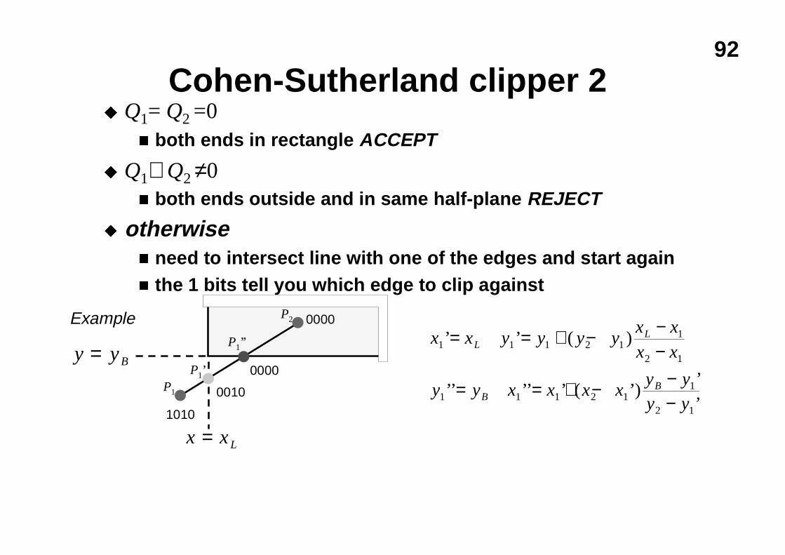
Cohen-Sutherland clipper 2u Q1= Q2 =0

n both ends in rectangle ACCEPT

u Q1∧ Q2 ≠0n both ends outside and in same half-plane REJECT

u otherwisen need to intersect line with one of the edges and start againn the 1 bits tell you which edge to clip against

y yB=

x x L=

0000

0010

1010

0000

x x y y y yx x

x x

y y x x x xy yy y

LL

BB

1 1 1 2 11

2 1

1 1 1 2 11

2 1

’ ’ ( )

’’ ’’ ’ ( ’)’’

= = + − −−

= = + − −−

P1

P1’

P1’’

P2Example

93

Cohen-Sutherland clipper 3u if code has more than a single 1 then you cannot tell

which is the best: simply select one and loop againu horizontal and vertical lines are not a problemu need a line drawing algorithm that can cope with

floating-point endpoint co-ordinates

y yT=

y yB=

x x L= x x R=

Why not?

Exercise: what happens in each ofthe cases at left?[Assume that, where there is achoice, the algorithm always trys tointersect with xL or xR before yB or yT.]

Try some other cases of your owndevising.

Why?

94

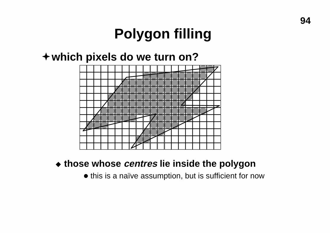
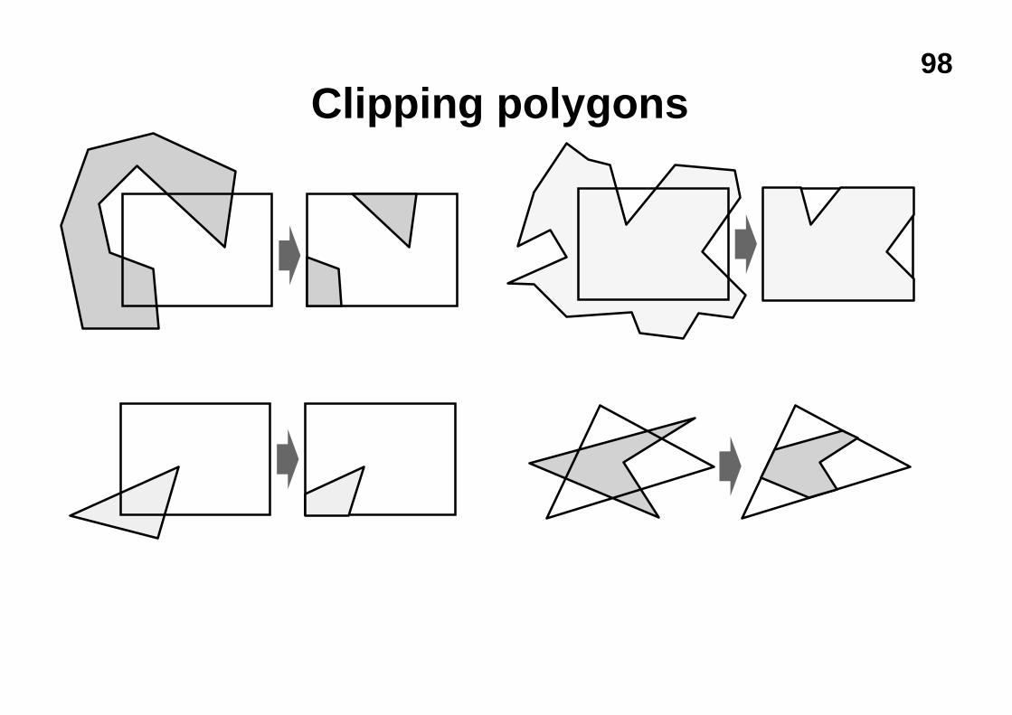
�which pixels do we turn on?

u those whose centres lie inside the polygonl this is a naïve assumption, but is sufficient for now

Polygon filling

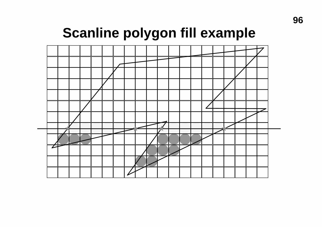
95Scanline polygon fill algorithm

ètake all polygon edges and place in an edge list (EL) , sorted onlowest y value

�start with the first scanline that intersects the polygon, get alledges which intersect that scan line and move them to an activeedge list (AEL)

�for each edge in the AEL: find the intersection point with thecurrent scanline; sort these into ascending order on the x value

�fill between pairs of intersection points�move to the next scanline (increment y); remove edges from

the AEL if endpoint < y ; move new edges from EL to AEL if startpoint ≤ y; if any edges remain in the AEL go back to step �

96

Scanline polygon fill example

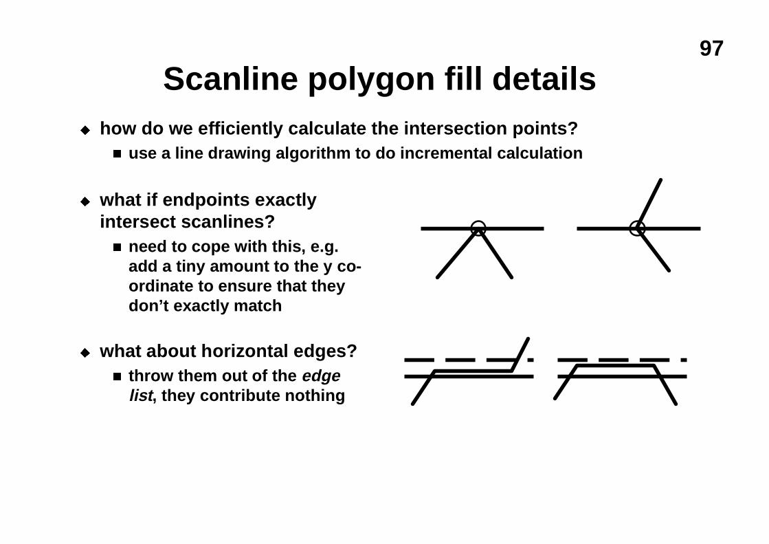
97

Scanline polygon fill detailsu how do we efficiently calculate the intersection points?

n use a line drawing algorithm to do incremental calculation

u what if endpoints exactlyintersect scanlines?n need to cope with this, e.g.

add a tiny amount to the y co-ordinate to ensure that theydon’t exactly match

u what about horizontal edges?n throw them out of the edge

list, they contribute nothing

98

Clipping polygons

99

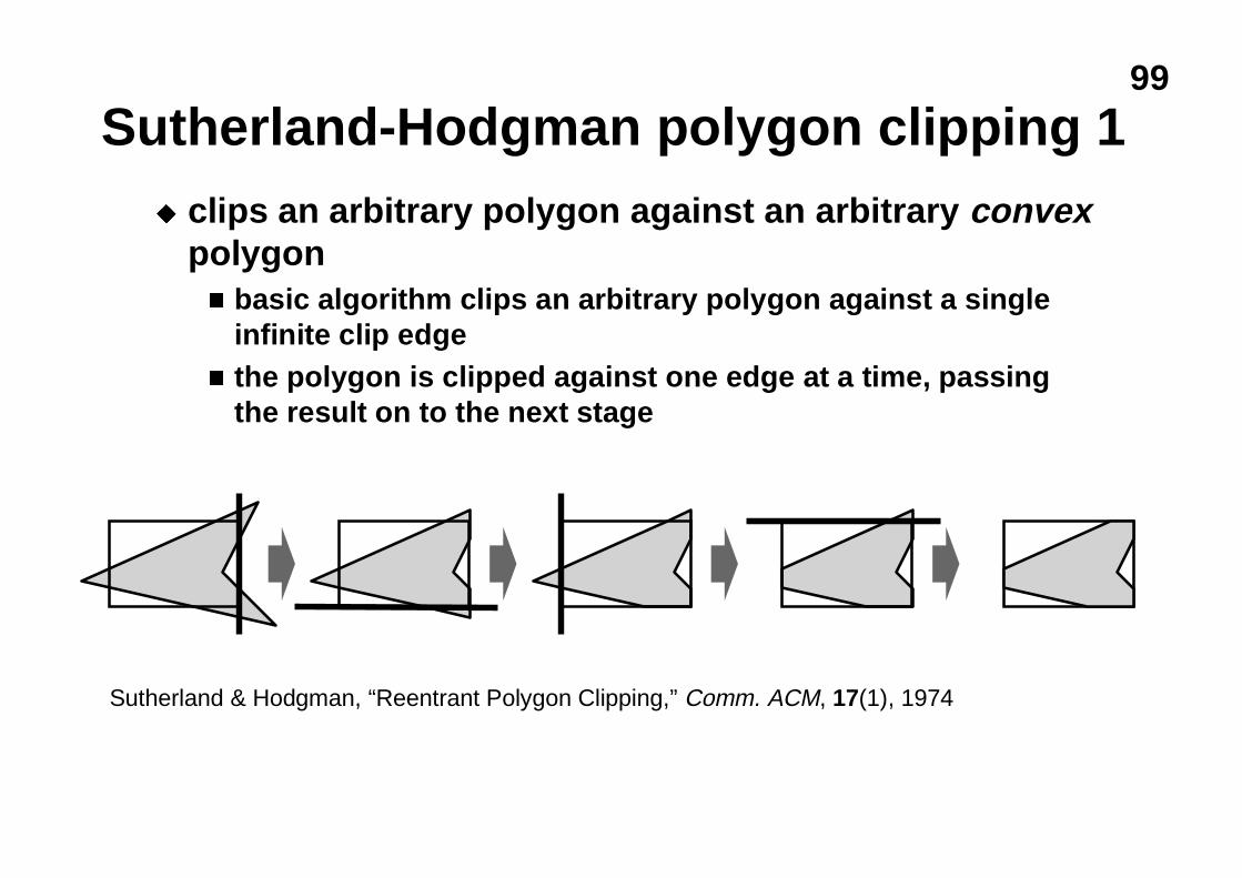
Sutherland-Hodgman polygon clipping 1u clips an arbitrary polygon against an arbitrary convex

polygonn basic algorithm clips an arbitrary polygon against a single

infinite clip edgen the polygon is clipped against one edge at a time, passing

the result on to the next stage

Sutherland & Hodgman, “Reentrant Polygon Clipping,” Comm. ACM, 17(1), 1974

100

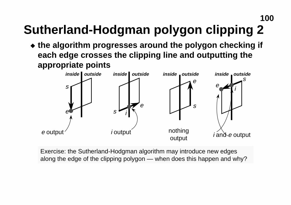
Sutherland-Hodgman polygon clipping 2u the algorithm progresses around the polygon checking if

each edge crosses the clipping line and outputting theappropriate points

s

e

e output

inside outside

se

i output

inside outsides

e

i and e output

inside outside

s

e

nothingoutput

inside outside

Exercise: the Sutherland-Hodgman algorithm may introduce new edgesalong the edge of the clipping polygon — when does this happen and why?

i

i

101

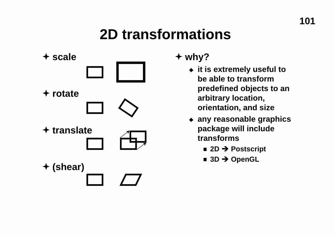
2D transformations� scale

� rotate

� translate

� (shear)

�why?u it is extremely useful to

be able to transformpredefined objects to anarbitrary location,orientation, and size

u any reasonable graphicspackage will includetransformsn 2D Ð Postscriptn 3D Ð OpenGL

102

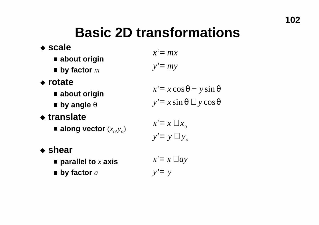
Basic 2D transformationsu scale

n about originn by factor m

u rotaten about originn by angle θ

u translaten along vector (xo,yo)

u shearn parallel to x axisn by factor a

x mx

y my

’

’

==

x x y

y x y

’ cos sin

’ sin cos

= −= +

θ θθ θ

x x x

y y yo

o

’

’

= += +

x x ay

y y

’

’

= +=

103

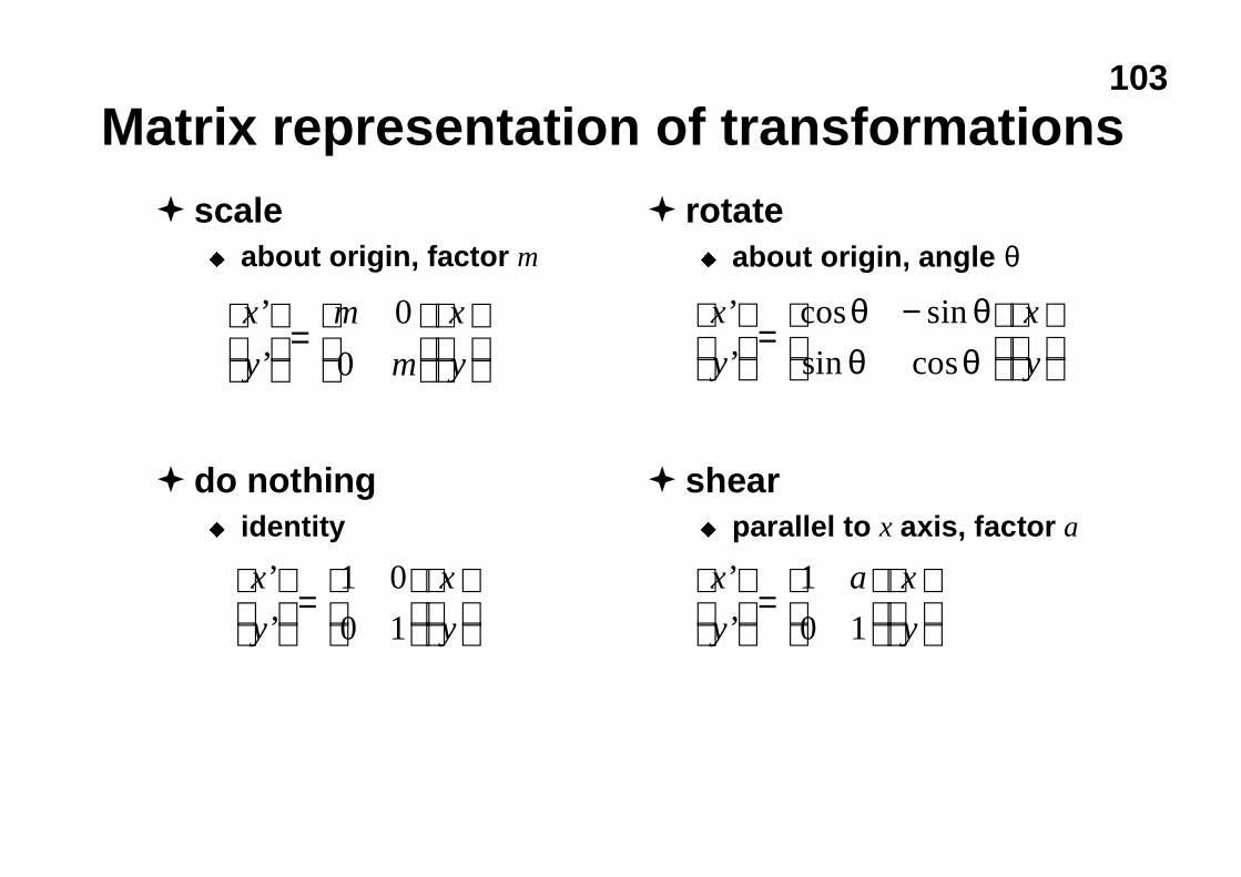
Matrix representation of transformations� scale

u about origin, factor m

� do nothingu identity

x

y

m

m

x

y

’

’

=

0

0

x

y

x

y

’

’

=

1 0

0 1

x

y

a x

y

’

’

=

1

0 1

� rotateu about origin, angle θ

� shearu parallel to x axis, factor a

x

y

x

y

’

’

cos sin

sin cos

=−

θ θθ θ

104

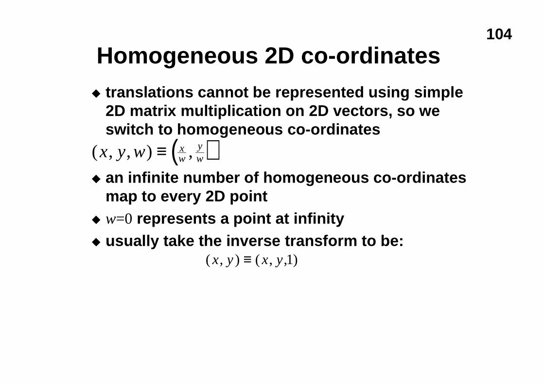
Homogeneous 2D co-ordinatesu translations cannot be represented using simple

2D matrix multiplication on 2D vectors, so weswitch to homogeneous co-ordinates

u an infinite number of homogeneous co-ordinatesmap to every 2D point

u w=0 represents a point at infinityu usually take the inverse transform to be:

( )( , , ) ,x y w xw

yw≡

( , ) ( , , )x y x y≡ 1

105

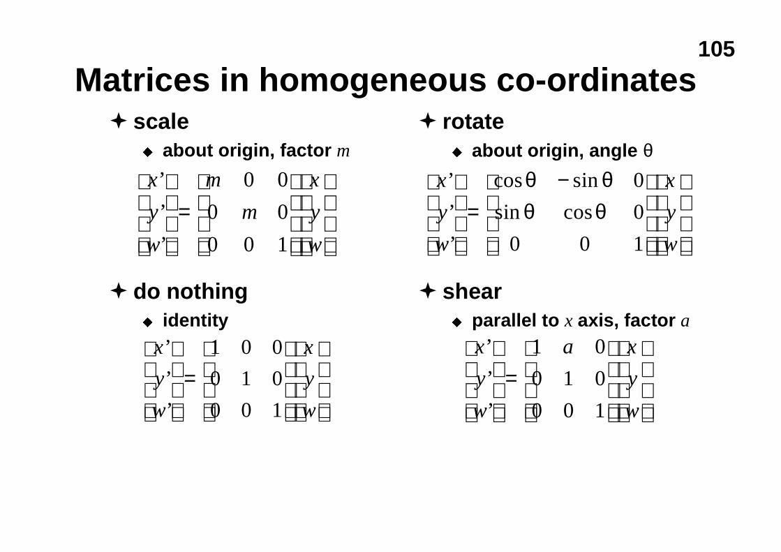
Matrices in homogeneous co-ordinates� scale

u about origin, factor m

� do nothingu identity

x

y

w

m

m

x

y

w

’

’

’

=

0 0

0 0

0 0 1

� rotateu about origin, angle θ

� shearu parallel to x axis, factor a

x

y

w

x

y

w

’

’

’

cos sin

sin cos

=−

θ θθ θ

0

0

0 0 1

x

y

w

a x

y

w

’

’

’

=

1 0

0 1 0

0 0 1

x

y

w

x

y

w

’

’

’

=

1 0 0

0 1 0

0 0 1

106

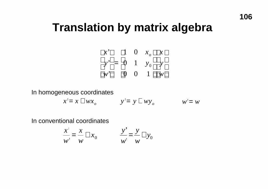
Translation by matrix algebra

x

y

w

x

y

x

y

w

o’

’

’

=

1 0

0 1

0 0 10

w w’=y y wyo’= +x x wxo’= +

xw

xw

x’’= + 0 0’

’y

w

y

w

y +=

In conventional coordinates

In homogeneous coordinates

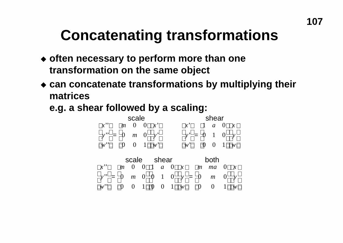
107

Concatenating transformationsu often necessary to perform more than one

transformation on the same objectu can concatenate transformations by multiplying their

matricese.g. a shear followed by a scaling:

x

y

w

m

m

x

y

w

x

y

w

a x

y

w

’’

’’

’’

’

’

’

’

’

’

=

=

0 0

0 0

0 0 1

1 0

0 1 0

0 0 1

x

y

w

m

m

a x

y

w

m ma

m

x

y

w

’’

’’

’’

=

=

0 0

0 0

0 0 1

1 0

0 1 0

0 0 1

0

0 0

0 0 1

shearscale

shearscale both

108

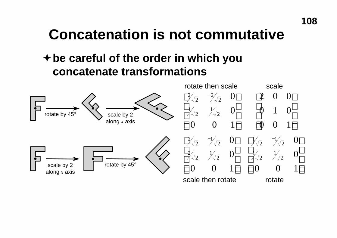
Concatenation is not commutative

�be careful of the order in which youconcatenate transformations

rotate by 45°

scale by 2along x axis

rotate by 45°

scale by 2along x axis

22

22

12

12

22

12

22

12

12

12

12

12

0

0

0 0 1

2 0 0

0 1 0

0 0 1

0

0

0 0 1

0

0

0 0 1

−

− −

scale

rotatescale then rotate

rotate then scale

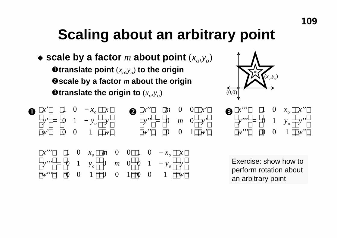
109

Scaling about an arbitrary pointu scale by a factor m about point (xo,yo)

ètranslate point (xo,yo) to the origin�scale by a factor m about the origin�translate the origin to (xo,yo)

(xo,yo)

(0,0)

x

y

w

x

y

x

y

w

o

o

’

’

’

=−−

1 0

0 1

0 0 1

x

y

w

m

m

x

y

w

’’

’’

’’

’

’

’

=

0 0

0 0

0 0 1

x

y

w

x

y

x

y

w

o

o

’’’

’’’

’’’

’’

’’

’’

=

1 0

0 1

0 0 1

x

y

w

x

y

m

m

x

y

x

y

w

o

o

o

o

’’’

’’’

’’’

=

−−

1 0

0 1

0 0 1

0 0

0 0

0 0 1

1 0

0 1

0 0 1

Exercise: show how toperform rotation aboutan arbitrary point

è � �

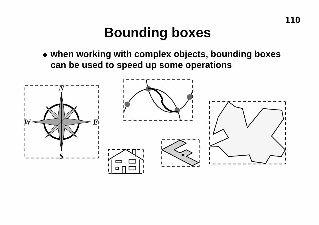
110

Bounding boxesu when working with complex objects, bounding boxes

can be used to speed up some operations

N

S

EW

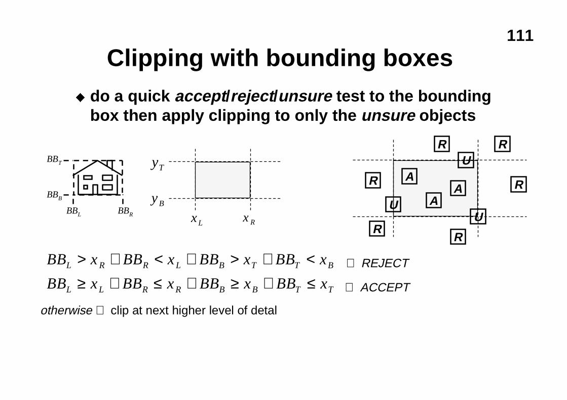
111

Clipping with bounding boxesu do a quick accept/reject/unsure test to the bounding

box then apply clipping to only the unsure objects

BBL BBR

BBB

BBT yT

yB

x L x R

A

AA

R R

R

RR

R

UU

U

BB x BB x BB x BB xL R R L B T T B> ∨ < ∨ > ∨ <BB x BB x BB x BB xL L R R B B T T≥ ∧ ≤ ∧ ≥ ∧ ≤

otherwise ⇒ clip at next higher level of detal

⇒ REJECT

⇒ ACCEPT

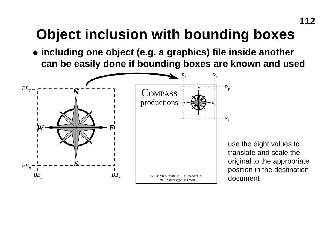
112

Object inclusion with bounding boxesu including one object (e.g. a graphics) file inside another

can be easily done if bounding boxes are known and used

use the eight values totranslate and scale theoriginal to the appropriateposition in the destinationdocument

N

S

EW

BBL BBR

BBB

BBTN

S

EW

COMPASSproductions

Tel: 01234 567890 Fax: 01234 567899E-mail: compass@piped.co.uk

PT

PB

PRPL

113

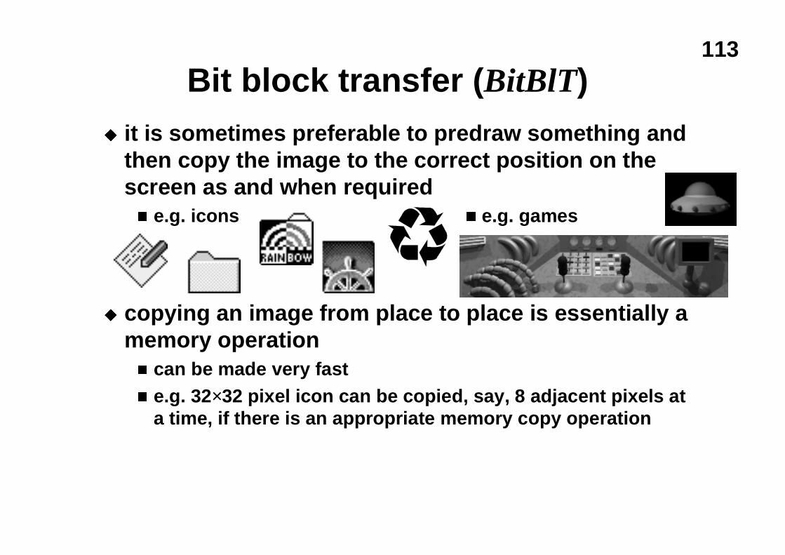
Bit block transfer (BitBlT)u it is sometimes preferable to predraw something and

then copy the image to the correct position on thescreen as and when requiredn e.g. icons n e.g. games

u copying an image from place to place is essentially amemory operationn can be made very fastn e.g. 32×32 pixel icon can be copied, say, 8 adjacent pixels at

a time, if there is an appropriate memory copy operation

114

XOR drawingu generally we draw objects in the appropriate colours,

overwriting what was already thereu sometimes, usually in HCI, we want to draw something

temporarily, with the intention of wiping it out (almost)immediately e.g. when drawing a rubber-band line

u if we bitwise XOR the object’s colour with the colouralready in the frame buffer we will draw an object of thecorrect shape (but wrong colour)

u if we do this twice we will restore the original framebuffer

u saves drawing the whole screen twice

115

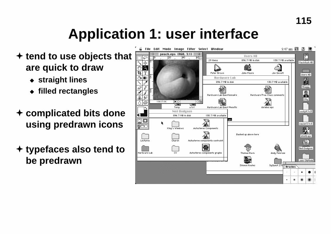
Application 1: user interface� tend to use objects that

are quick to drawu straight linesu filled rectangles

� complicated bits doneusing predrawn icons

� typefaces also tend tobe predrawn

116

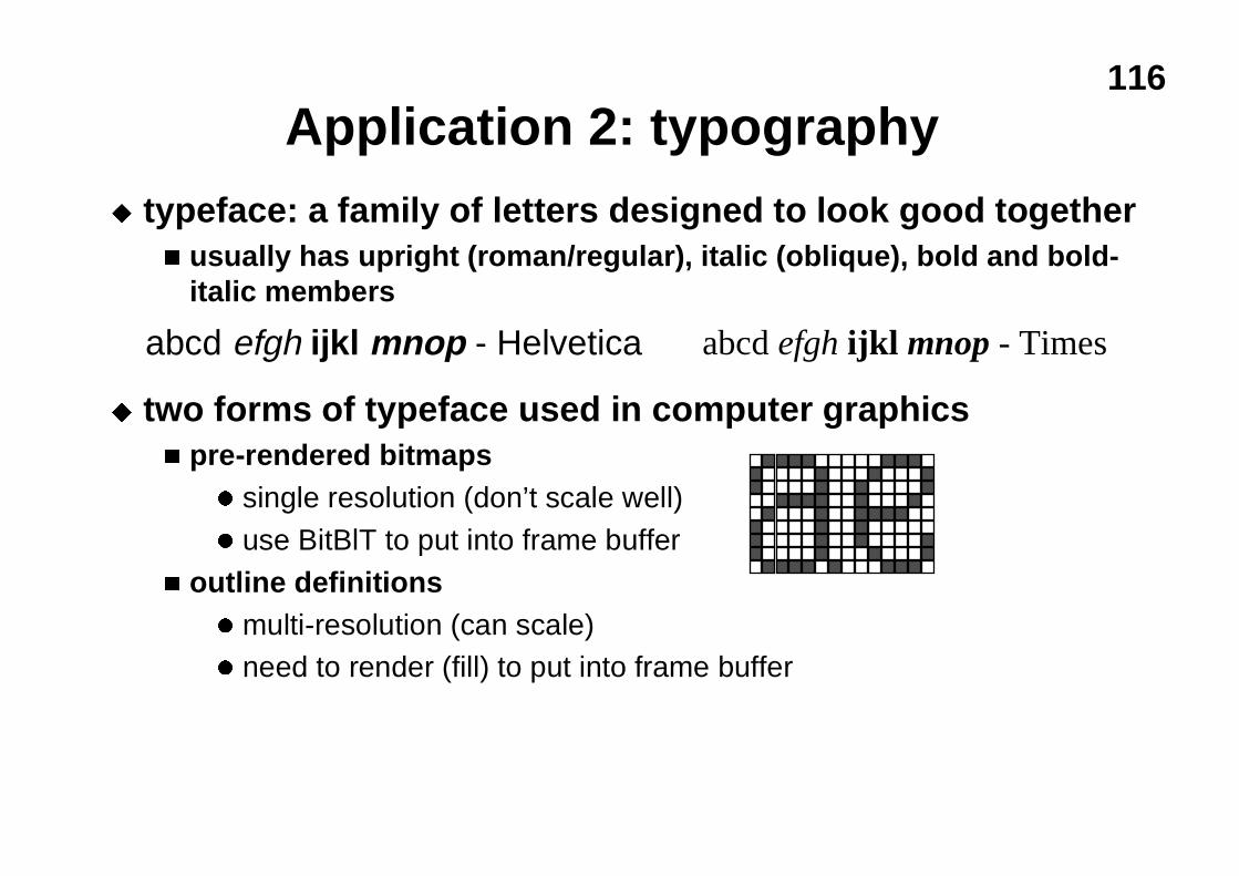
Application 2: typographyu typeface: a family of letters designed to look good together

n usually has upright (roman/regular), italic (oblique), bold and bold-italic members

u two forms of typeface used in computer graphicsn pre-rendered bitmaps

l single resolution (don’t scale well)

l use BitBlT to put into frame buffer

n outline definitionsl multi-resolution (can scale)l need to render (fill) to put into frame buffer

abcd efgh ijkl mnop - Helvetica abcd efgh ijkl mnop - Times

117

Application 3: Postscriptu industry standard rendering language for printersu developed by Adobe Systemsu stack-based interpreted languageu basic features

n object outlines made up of lines, arcs & Bezier curvesn objects can be filled or strokedn whole range of 2D transformations can be applied to

objectsn typeface handling built inn halftoningn can define your own functions in the language

118

3D Computer Graphics�3D Ø 2D projection�3D versions of 2D operations

u clipping, transforms, matrices, curves & surfaces

�3D scan conversionu depth-sort, BSP tree, z-Buffer, A-buffer

�sampling�lighting�ray tracing

IP

Background

2D CG

3D CG

119

3D Ø 2D projection

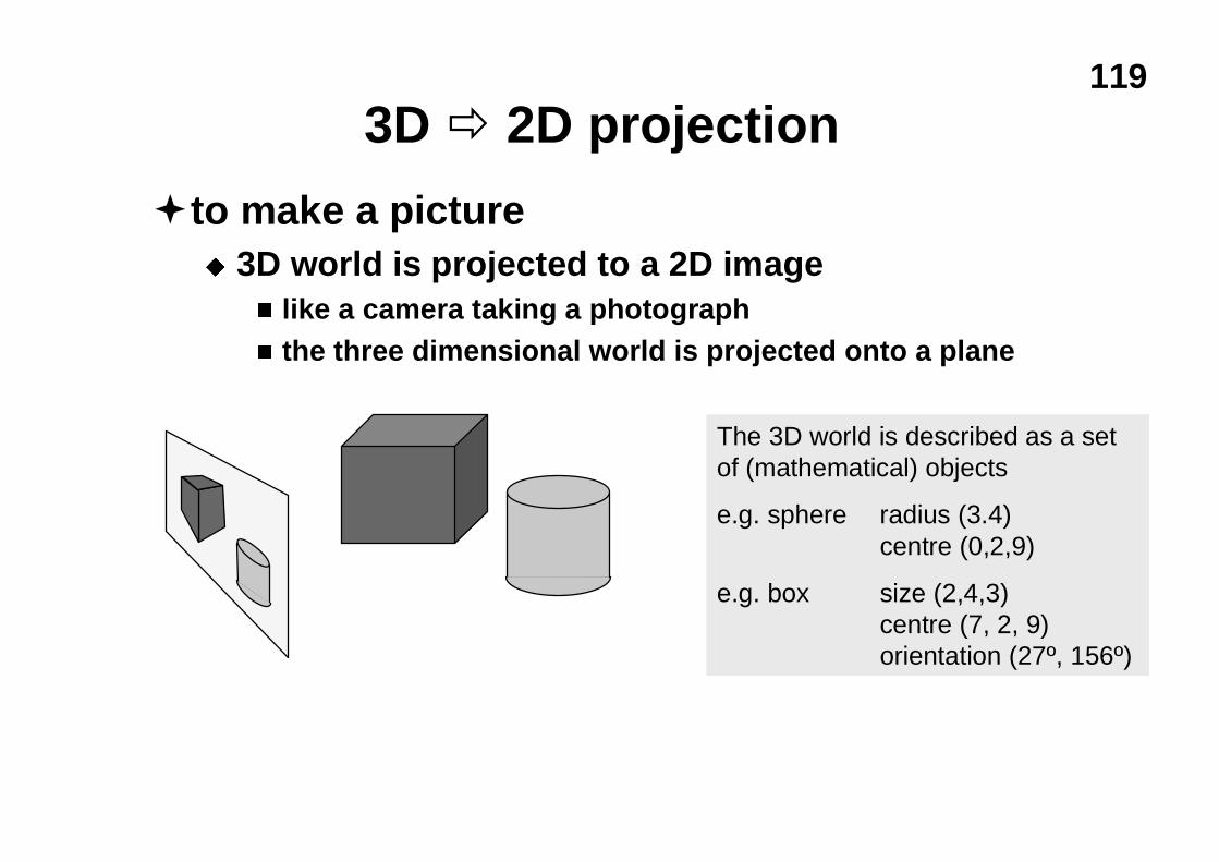
�to make a pictureu 3D world is projected to a 2D image

n like a camera taking a photographn the three dimensional world is projected onto a plane

The 3D world is described as a setof (mathematical) objects

e.g. sphere radius (3.4)centre (0,2,9)

e.g. box size (2,4,3)centre (7, 2, 9)orientation (27º, 156º)

120

Types of projection

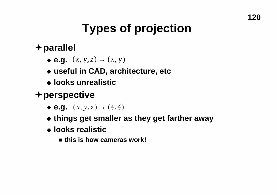
�parallelu e.g.u useful in CAD, architecture, etcu looks unrealistic

�perspectiveu e.g.u things get smaller as they get farther awayu looks realistic

n this is how cameras work!

( , , ) ( , )x y z x y→

( , , ) ( , )x y z xz

yz→

121

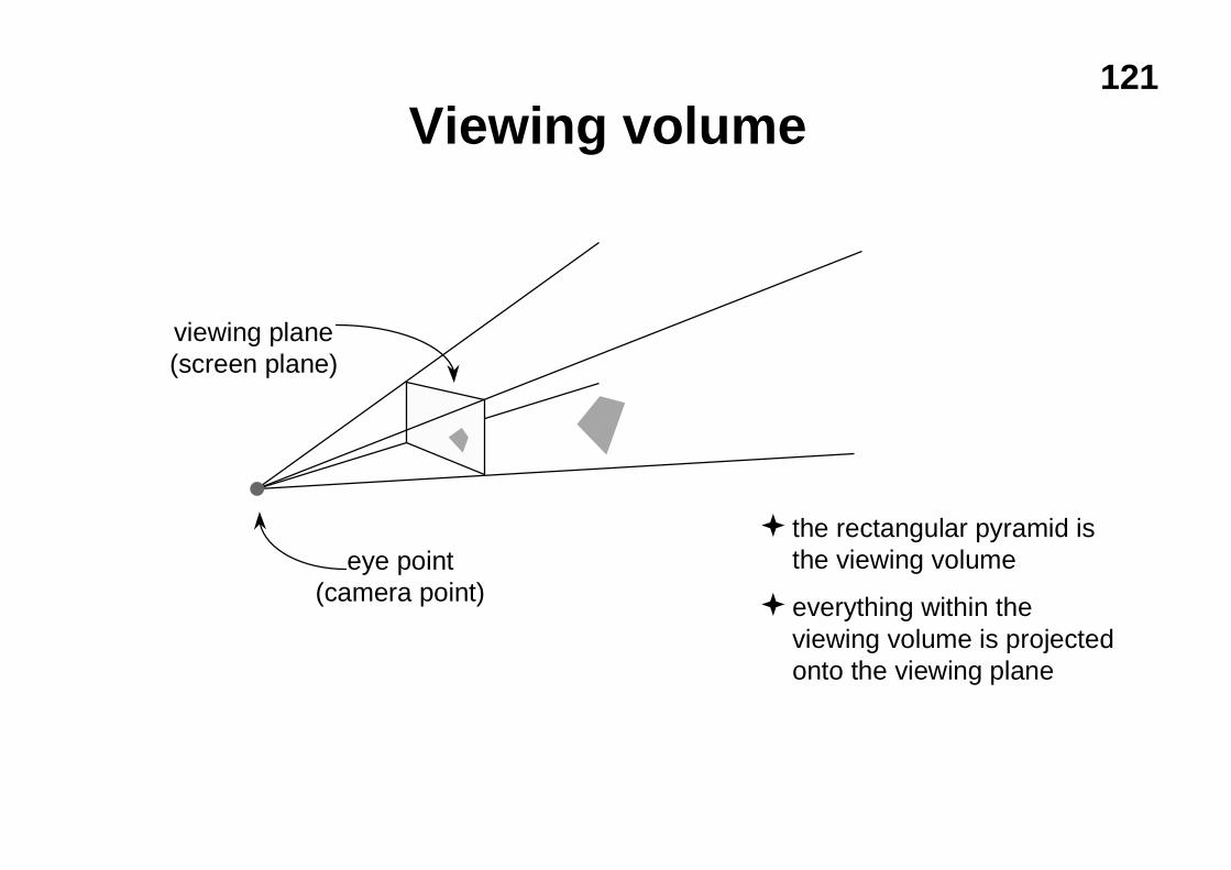
Viewing volume

eye point(camera point)

viewing plane(screen plane)

� the rectangular pyramid isthe viewing volume

� everything within theviewing volume is projectedonto the viewing plane

122

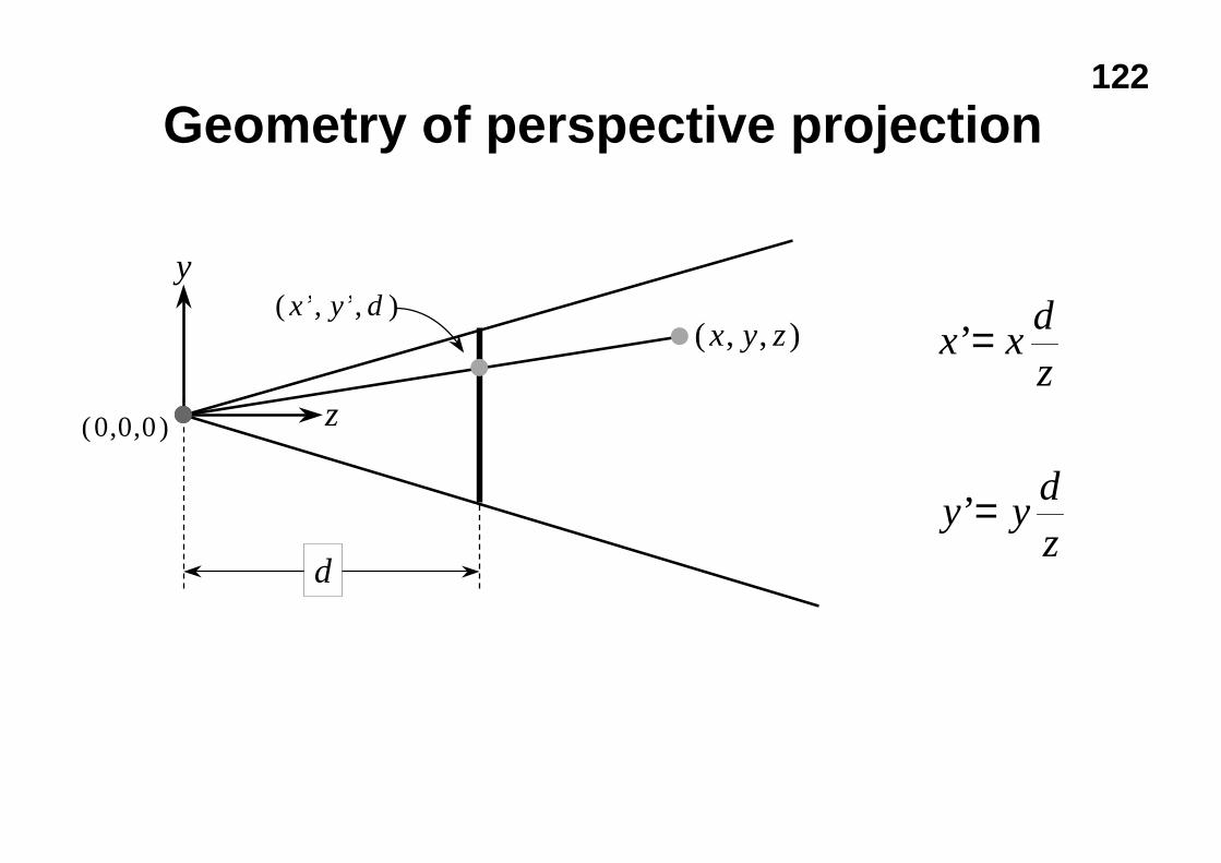
Geometry of perspective projection

y

z

d

( , , )x y z( ’, ’, )x y d

x xd

z

y yd

z

’

’

=

=

( , , )0 0 0

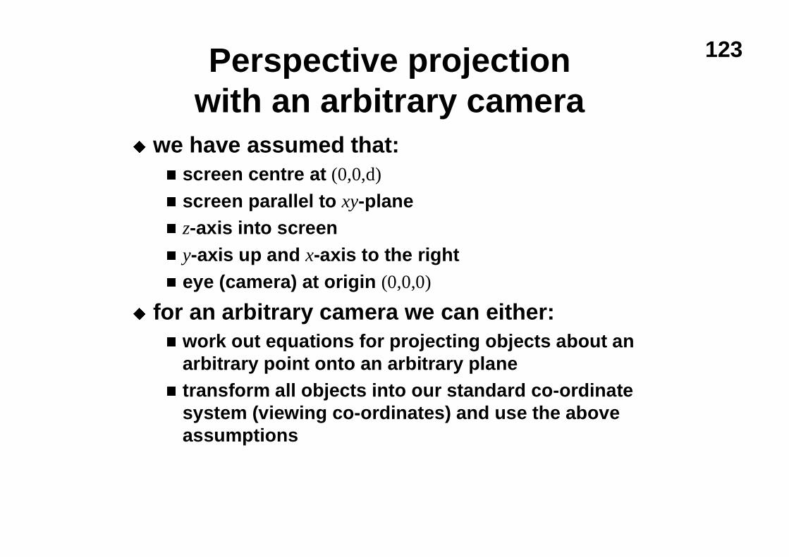
123Perspective projectionwith an arbitrary camera

u we have assumed that:n screen centre at (0,0,d)

n screen parallel to xy-planen z-axis into screenn y-axis up and x-axis to the rightn eye (camera) at origin (0,0,0)

u for an arbitrary camera we can either:n work out equations for projecting objects about an

arbitrary point onto an arbitrary planen transform all objects into our standard co-ordinate

system (viewing co-ordinates) and use the aboveassumptions

124

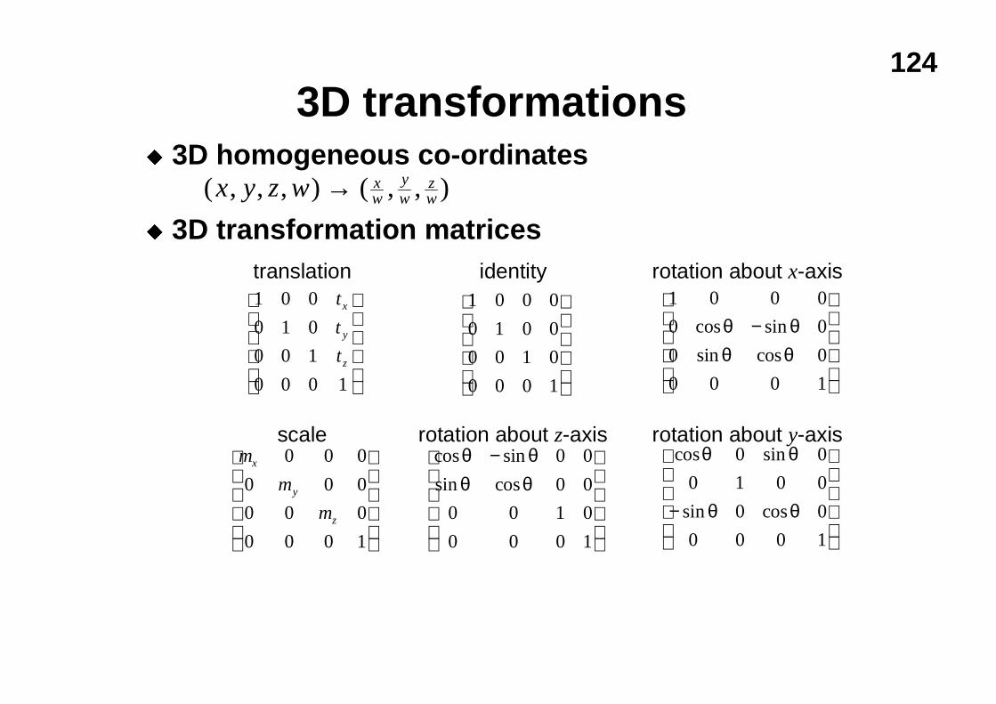
3D transformationsu 3D homogeneous co-ordinates

u 3D transformation matrices

( , , , ) ( , , )x y z w xw

yw

zw→

1 0 0 0

0 1 0 0

0 0 1 0

0 0 0 1

m

m

m

x

y

z

0 0 0

0 0 0

0 0 0

0 0 0 1

1 0 0

0 1 0

0 0 1

0 0 0 1

t

t

t

x

y

z

cos sin

sin cos

θ θθ θ

−

0 0

0 0

0 0 1 0

0 0 0 1

1 0 0 0

0 0

0 0

0 0 0 1

cos sin

sin cos

θ θθ θ

−

cos sin

sin cos

θ θ

θ θ

0 0

0 1 0 0

0 0

0 0 0 1

−

translation identity

scale

rotation about x-axis

rotation about y-axisrotation about z-axis

125

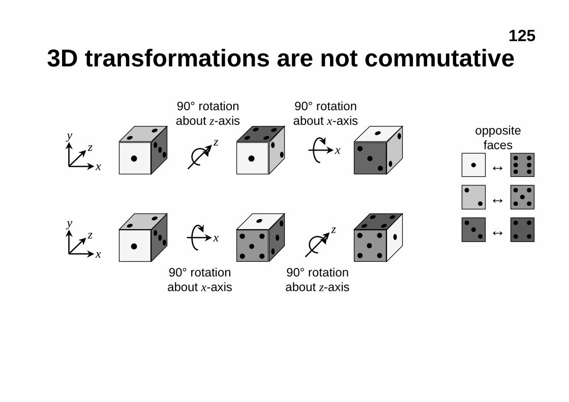
3D transformations are not commutative

x

yz

x

xz

z

x

yz

90° rotationabout z-axis

90° rotationabout x-axis

90° rotationabout z-axis

90° rotationabout x-axis

oppositefaces

↔

↔

↔

126

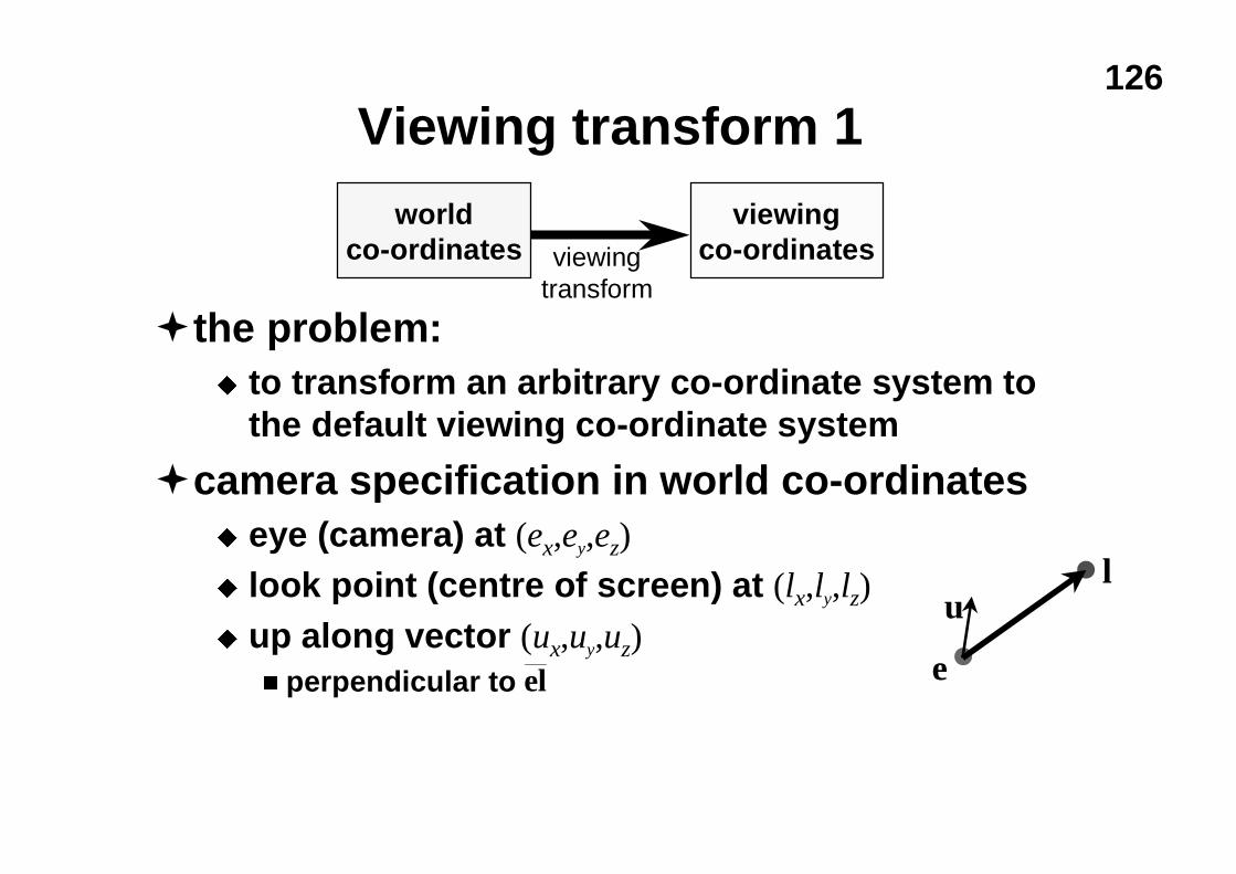
Viewing transform 1

�the problem:u to transform an arbitrary co-ordinate system to

the default viewing co-ordinate system

�camera specification in world co-ordinatesu eye (camera) at (ex,ey,ez)

u look point (centre of screen) at (lx,ly,lz)

u up along vector (ux,uy,uz)n perpendicular to

worldco-ordinates

viewingco-ordinatesviewing

transform

u

e

l

el

127

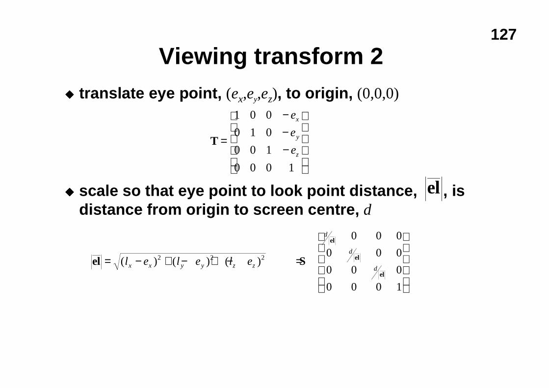
Viewing transform 2u translate eye point, (ex,ey,ez), to origin, (0,0,0)

u scale so that eye point to look point distance, , isdistance from origin to screen centre, d

el

T =

−−−

1 0 0

0 1 0

0 0 1

0 0 0 1

e

e

e

x

y

z

el S

el

el

el

= − + − + − =

( ) ( ) ( )l e l e l ex x y y z z

d

d

d

2 2 2

0 0 0

0 0 0

0 0 0

0 0 0 1

128

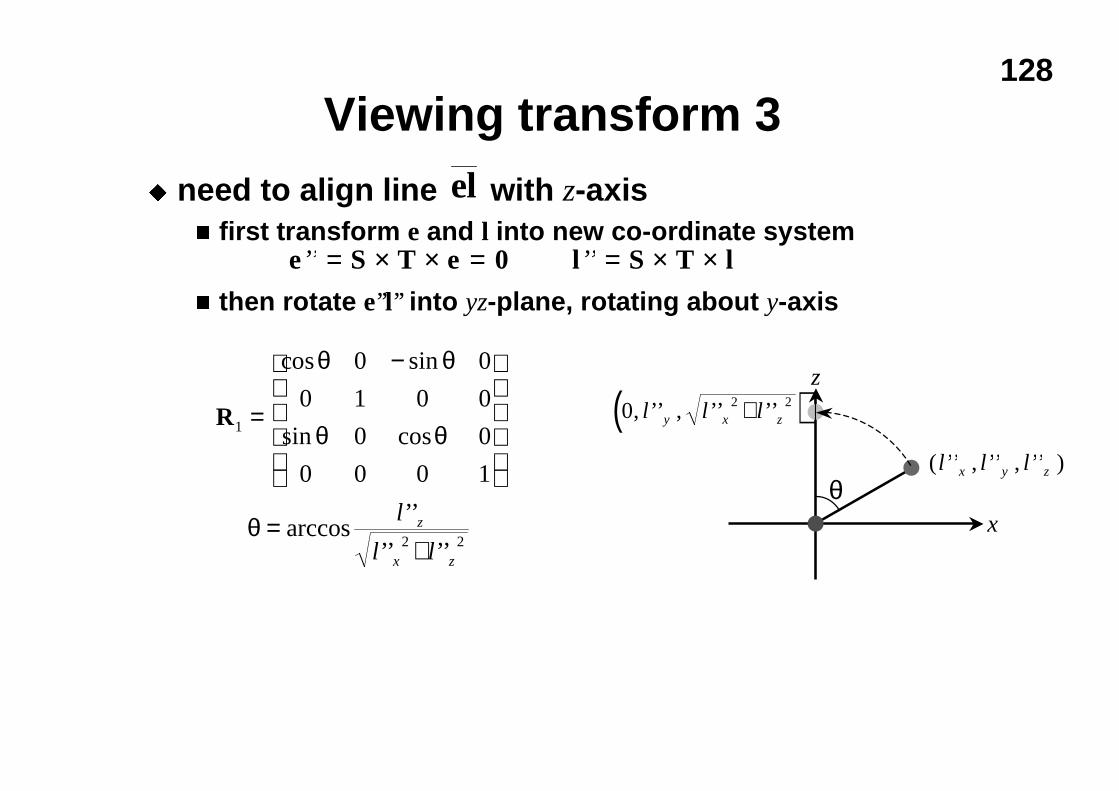
Viewing transform 3u need to align line with z-axis

n first transform e and l into new co-ordinate system

n then rotate e’’l’’ into yz-plane, rotating about y-axis

el

e S T e 0 l S T l’’ ’’= × × = = × ×

R1

2 2

0 0

0 1 0 0

0 0

0 0 0 1

=

−

=+

cos sin

sin cos

arccos’’

’’ ’’

θ θ

θ θ

θ l

l lz

x z

x

z

( ’’ , ’’ , ’’ )l l lx y z

( )0 2 2, ’’ , ’’ ’’l l ly x z+

θ

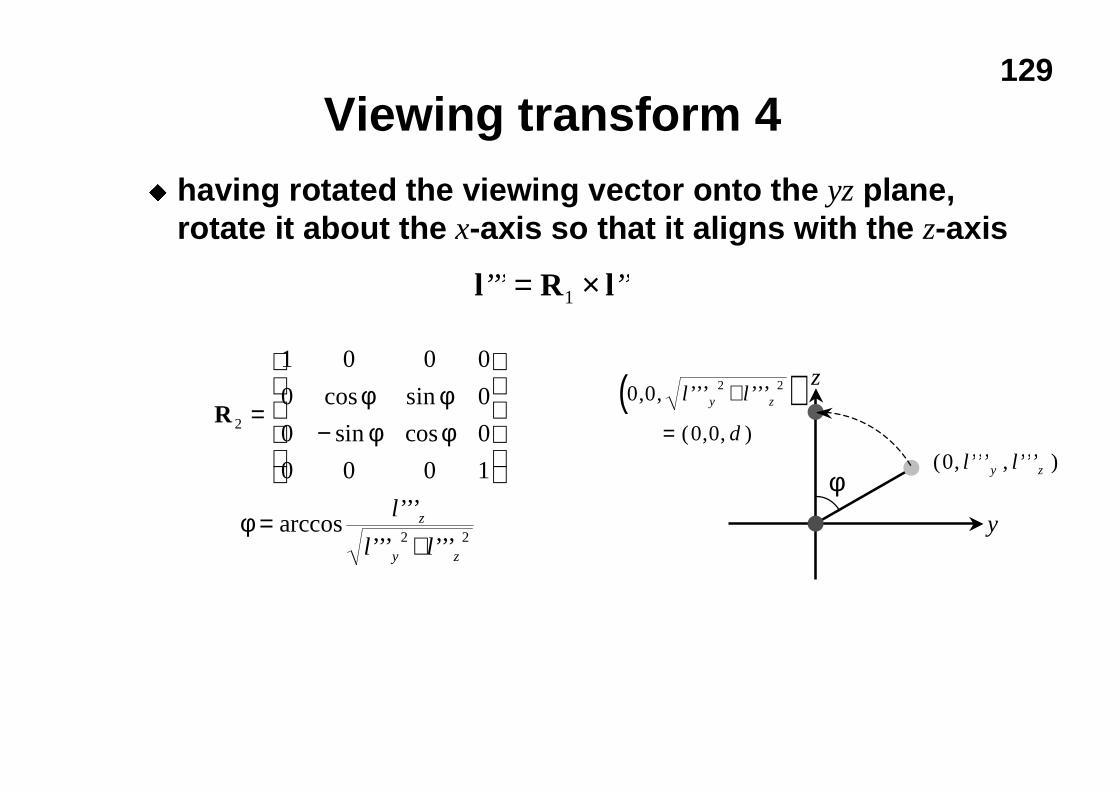
129

Viewing transform 4u having rotated the viewing vector onto the yz plane,

rotate it about the x-axis so that it aligns with the z-axis

R 2

2 2

1 0 0 0

0 0

0 0

0 0 0 1

=−

=+

cos sin

sin cos

arccos’’’

’’’ ’’’

φ φφ φ

φ l

l lz

y z

y

z

( , ’’’ , ’’’ )0 l ly z

( )0 0

0 0

2 2, , ’’’ ’’’

( , , )

l l

d

y z+

=

φ

l R l’’’ ’’= ×1

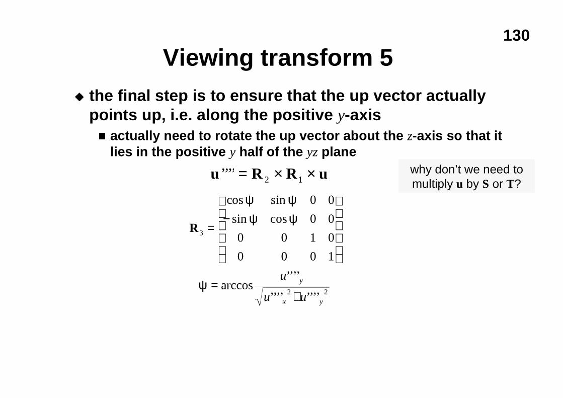
130

Viewing transform 5u the final step is to ensure that the up vector actually

points up, i.e. along the positive y-axisn actually need to rotate the up vector about the z-axis so that it

lies in the positive y half of the yz plane

u R R u’’’’ = × ×2 1why don’t we need tomultiply u by S or T?

R3

2 2

0 0

0 0

0 0 1 0

0 0 0 1

=−

=+

cos sin

sin cos

arccos’’’’

’’’’ ’’’’

ψ ψψ ψ

ψu

u u

y

x y

131

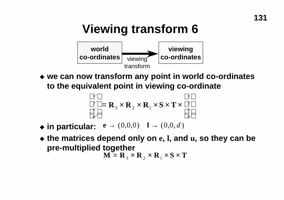
Viewing transform 6

u we can now transform any point in world co-ordinatesto the equivalent point in viewing co-ordinate

u in particular:u the matrices depend only on e, l, and u, so they can be

pre-multiplied together

worldco-ordinates

viewingco-ordinatesviewing

transform

x

y

z

w

x

y

z

w

’

’

’

’

= × × × × ×

R R R S T3 2 1

e l→ →( , , ) ( , , )0 0 0 0 0 d

M R R R S T= × × × ×3 2 1

132

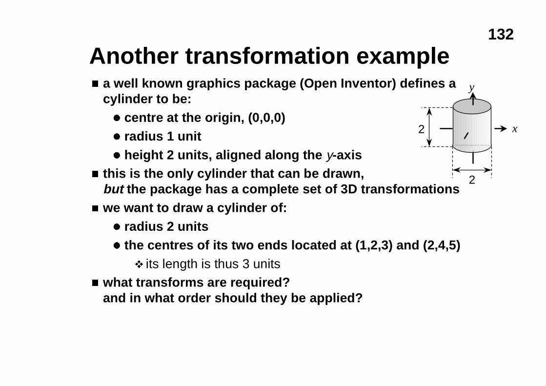
Another transformation examplen a well known graphics package (Open Inventor) defines a

cylinder to be:l centre at the origin, (0,0,0)l radius 1 unitl height 2 units, aligned along the y-axis

n this is the only cylinder that can be drawn,but the package has a complete set of 3D transformations

n we want to draw a cylinder of:l radius 2 unitsl the centres of its two ends located at (1,2,3) and (2,4,5)

v its length is thus 3 unitsn what transforms are required?

and in what order should they be applied?

x

y

2

2

133

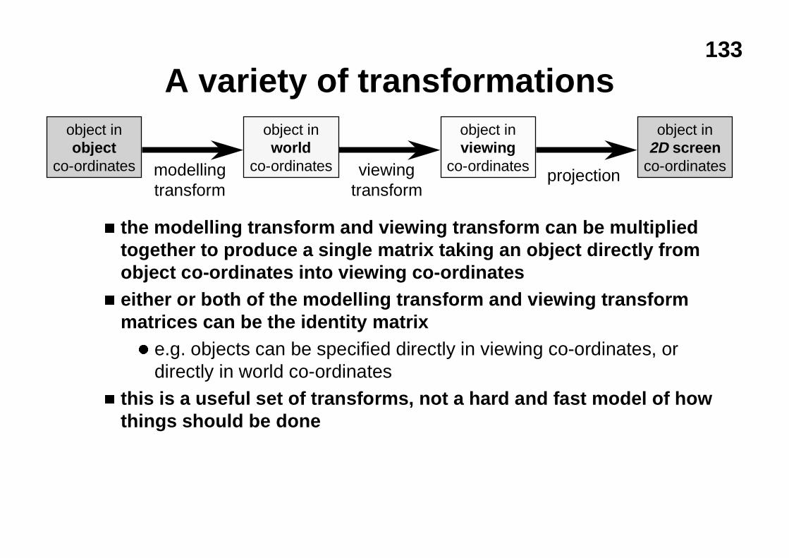
A variety of transformations

n the modelling transform and viewing transform can be multipliedtogether to produce a single matrix taking an object directly fromobject co-ordinates into viewing co-ordinates

n either or both of the modelling transform and viewing transformmatrices can be the identity matrixl e.g. objects can be specified directly in viewing co-ordinates, or

directly in world co-ordinates

n this is a useful set of transforms, not a hard and fast model of howthings should be done

object inworld

co-ordinates

object inviewing

co-ordinatesviewingtransform

object in2D screen

co-ordinatesprojection

object inobject

co-ordinates modellingtransform

134

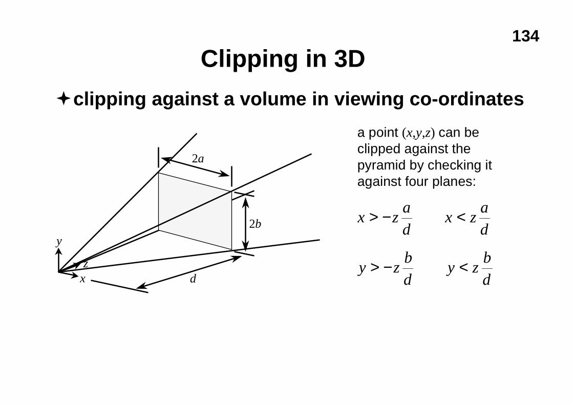
Clipping in 3D

�clipping against a volume in viewing co-ordinates

x

y

zd

2b

2a

a point (x,y,z) can beclipped against thepyramid by checking itagainst four planes:

x za

dx z

a

d

y zb

dy z

b

d

> − <

> − <

135

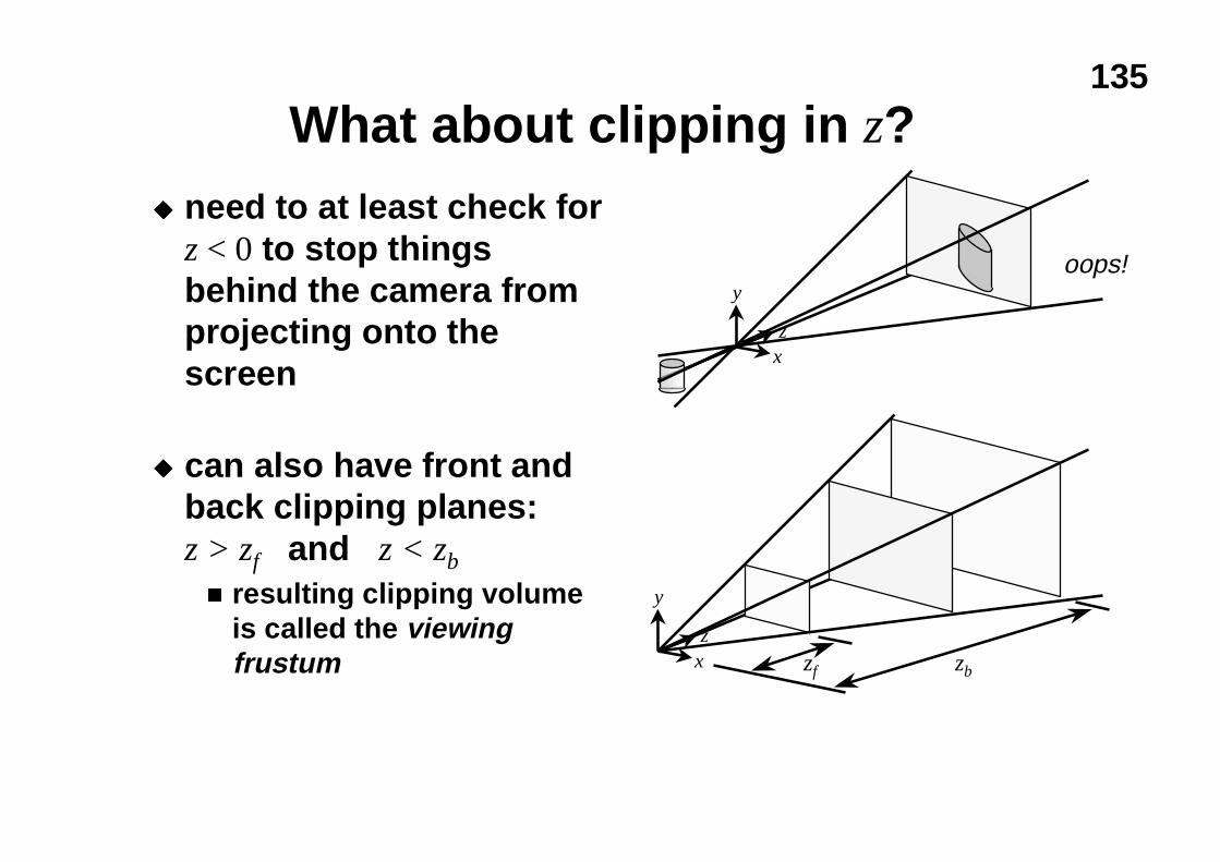
What about clipping in z?u need to at least check for

z < 0 to stop thingsbehind the camera fromprojecting onto thescreen

u can also have front andback clipping planes:z > zf and z < zb

n resulting clipping volumeis called the viewingfrustum zf

x

y

z

zb

x

y

z

oops!

136

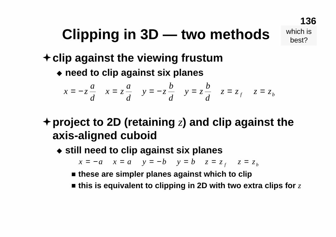
Clipping in 3D — two methods

�clip against the viewing frustumu need to clip against six planes

�project to 2D (retaining z) and clip against theaxis-aligned cuboidu still need to clip against six planes

n these are simpler planes against which to clipn this is equivalent to clipping in 2D with two extra clips for z

x za

dx z

a

dy z

b

dy z

b

dz z z zf b= − = = − = = =

x a x a y b y b z z z zf b= − = = − = = =

which isbest?

137

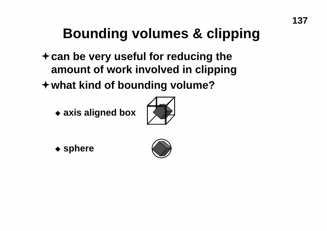
Bounding volumes & clipping

�can be very useful for reducing theamount of work involved in clipping

�what kind of bounding volume?

u axis aligned box

u sphere

138

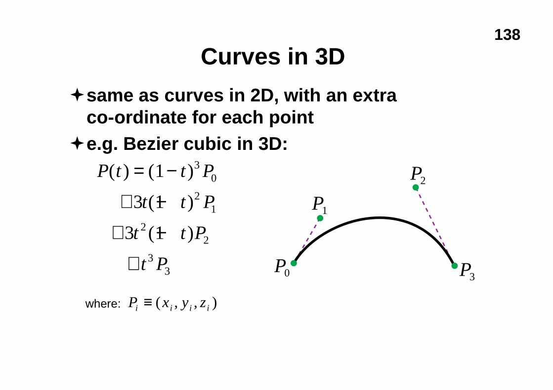
Curves in 3D

�same as curves in 2D, with an extraco-ordinate for each point

�e.g. Bezier cubic in 3D:P t t P

t t P

t t P

t P

( ) ( )

( )

( )

= −

+ −

+ −

+

1

3 1

3 1

30

21

22

33 P0

P1

P2

P3

where: P x y zi i i i≡ ( , , )

139

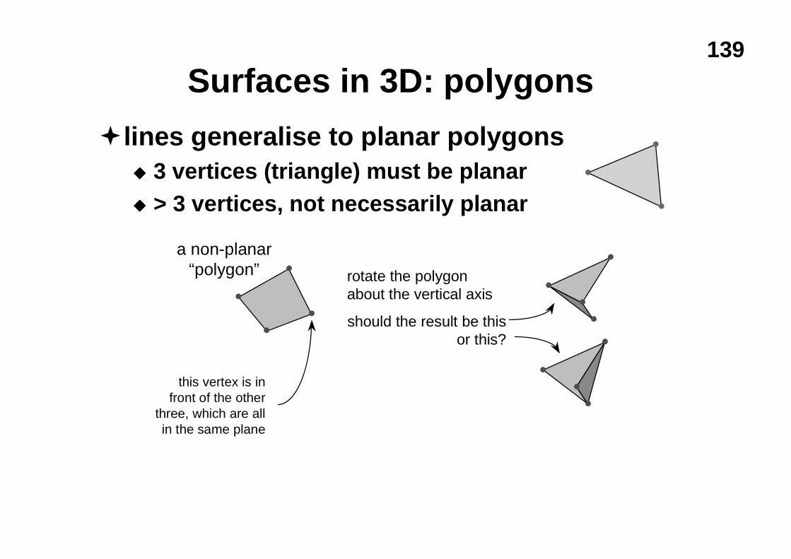
Surfaces in 3D: polygons

�lines generalise to planar polygonsu 3 vertices (triangle) must be planaru > 3 vertices, not necessarily planar

this vertex is infront of the other

three, which are allin the same plane

a non-planar“polygon” rotate the polygon

about the vertical axis

should the result be thisor this?

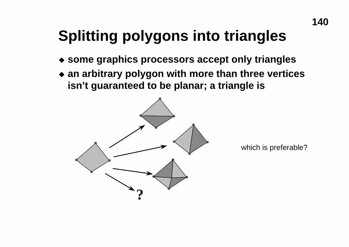
140

Splitting polygons into trianglesu some graphics processors accept only trianglesu an arbitrary polygon with more than three vertices

isn’t guaranteed to be planar; a triangle is

which is preferable?

?

141

Surfaces in 3D: patches

�curves generalise to patchesu a Bezier patch has a Bezier curve running along

each of its four edges and four extra internalcontrol points

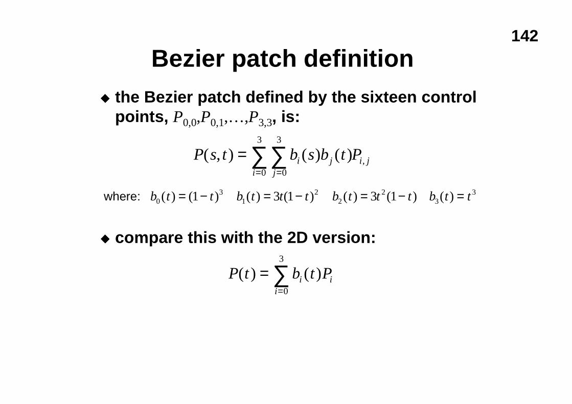
142

Bezier patch definitionu the Bezier patch defined by the sixteen control

points, P0,0,P0,1,…,P3,3, is:

u compare this with the 2D version:

b t t b t t t b t t t b t t03

12

22

331 3 1 3 1( ) ( ) ( ) ( ) ( ) ( ) ( )= − = − = − =

P s t b s b t Pi jji

i j( , ) ( ) ( ) ,===

∑∑0

3

0

3

where:

P t b t Pi ii

( ) ( )==∑

0

3

143

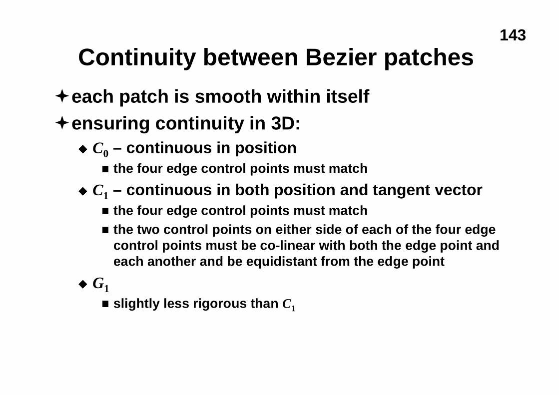
Continuity between Bezier patches

�each patch is smooth within itself�ensuring continuity in 3D:

u C0 – continuous in positionn the four edge control points must match

u C1 – continuous in both position and tangent vectorn the four edge control points must matchn the two control points on either side of each of the four edge

control points must be co-linear with both the edge point andeach another and be equidistant from the edge point

u G1

n slightly less rigorous than C1

144

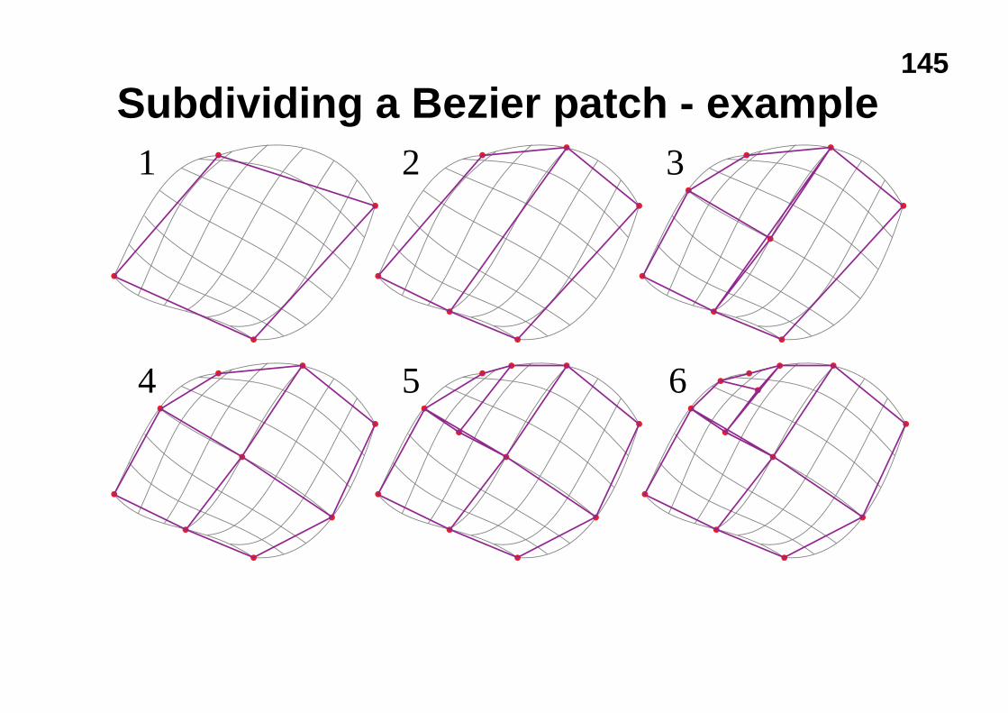
Drawing Bezier patchesu in a similar fashion to Bezier curves, Bezier patches can be

drawn by approximating them with planar polygonsu method:

n check if the Bezier patch is sufficiently well approximated by aquadrilateral, if so use that quadrilateral

n if not then subdivide it into two smaller Bezier patches and repeat oneachl subdivide in different dimensions on alternate calls to the subdivision

function

n having approximated the whole Bezier patch as a set of (non-planar)quadrilaterals, further subdivide these into (planar) trianglesl be careful to not leave any gaps in the resulting surface!

145

Subdividing a Bezier patch - example1 2 3

4 5 6

146

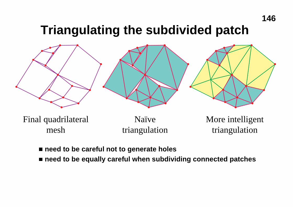
Triangulating the subdivided patch

Final quadrilateralmesh

Naïvetriangulation

More intelligenttriangulation

n need to be careful not to generate holesn need to be equally careful when subdividing connected patches

147

3D scan conversion

�lines�polygons

u depth sortu Binary Space-Partitioning treeu z-bufferu A-buffer

�ray tracing

148

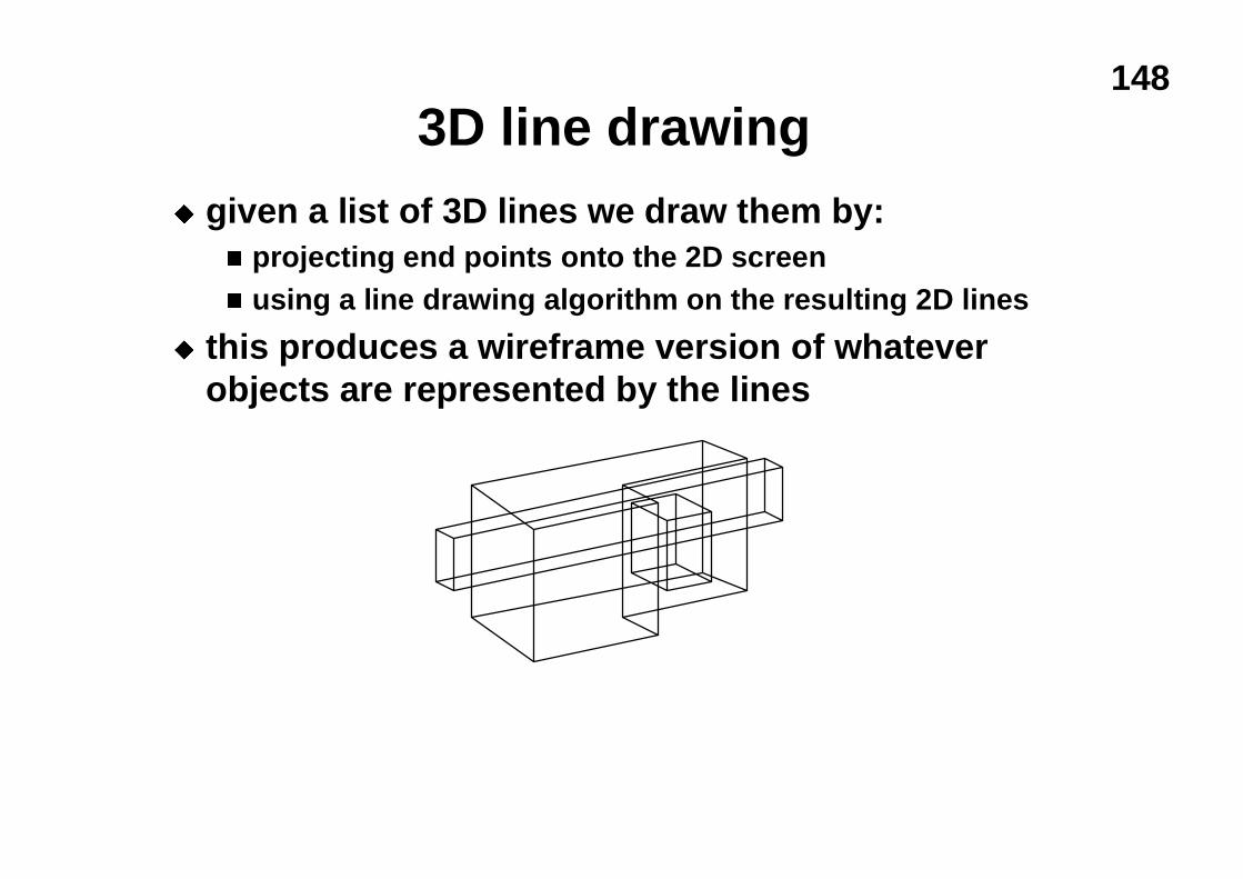
3D line drawingu given a list of 3D lines we draw them by:

n projecting end points onto the 2D screenn using a line drawing algorithm on the resulting 2D lines

u this produces a wireframe version of whateverobjects are represented by the lines

149

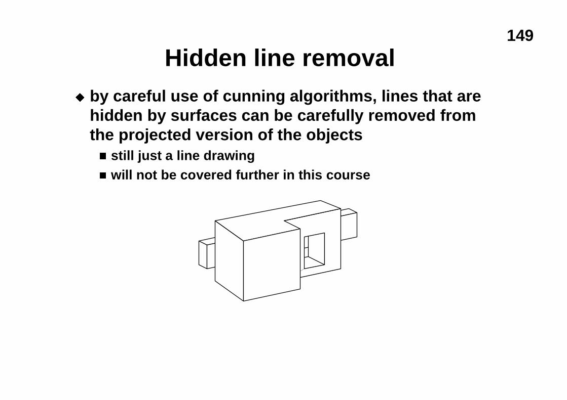
Hidden line removalu by careful use of cunning algorithms, lines that are

hidden by surfaces can be carefully removed fromthe projected version of the objectsn still just a line drawingn will not be covered further in this course

150

3D polygon drawingu given a list of 3D polygons we draw them by:

n projecting vertices onto the 2D screenl but also keep the z information

n using a 2D polygon scan conversion algorithm on theresulting 2D polygons

u in what order do we draw the polygons?n some sort of order on z

l depth sort

l Binary Space-Partitioning tree

u is there a method in which order does not matter?l z-buffer

151

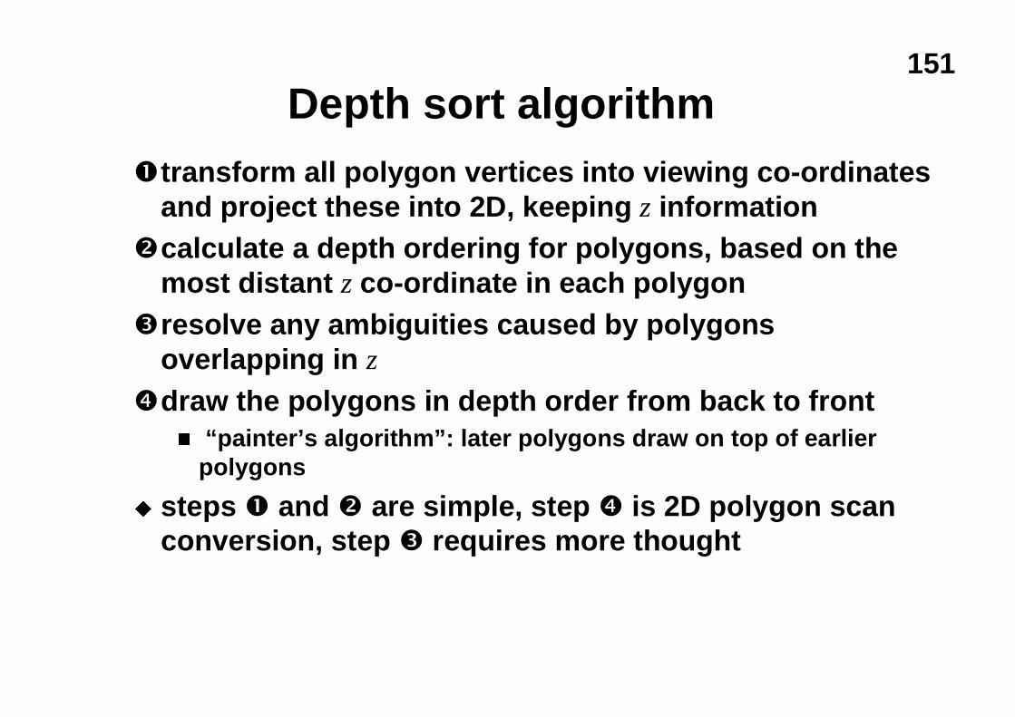
Depth sort algorithmètransform all polygon vertices into viewing co-ordinates

and project these into 2D, keeping z information�calculate a depth ordering for polygons, based on the

most distant z co-ordinate in each polygon�resolve any ambiguities caused by polygons

overlapping in z�draw the polygons in depth order from back to front

n “painter’s algorithm”: later polygons draw on top of earlierpolygons

u steps è and � are simple, step � is 2D polygon scanconversion, step � requires more thought

152

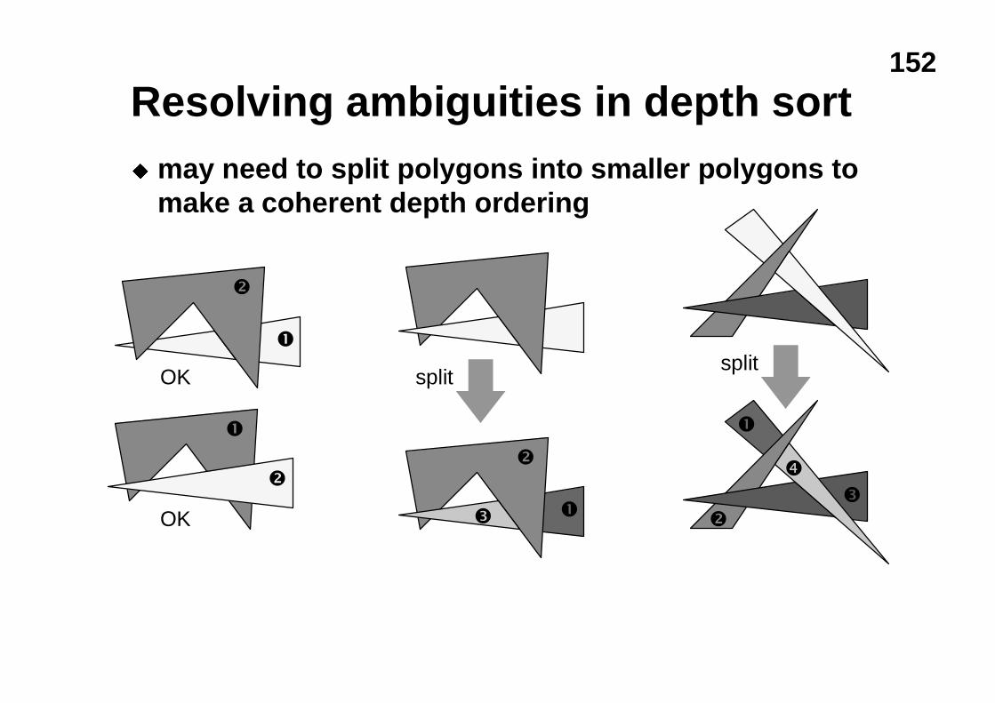
Resolving ambiguities in depth sortu may need to split polygons into smaller polygons to

make a coherent depth ordering

OK

OK

splitè

è

�

�

è

�

�

split

è

��

�

153

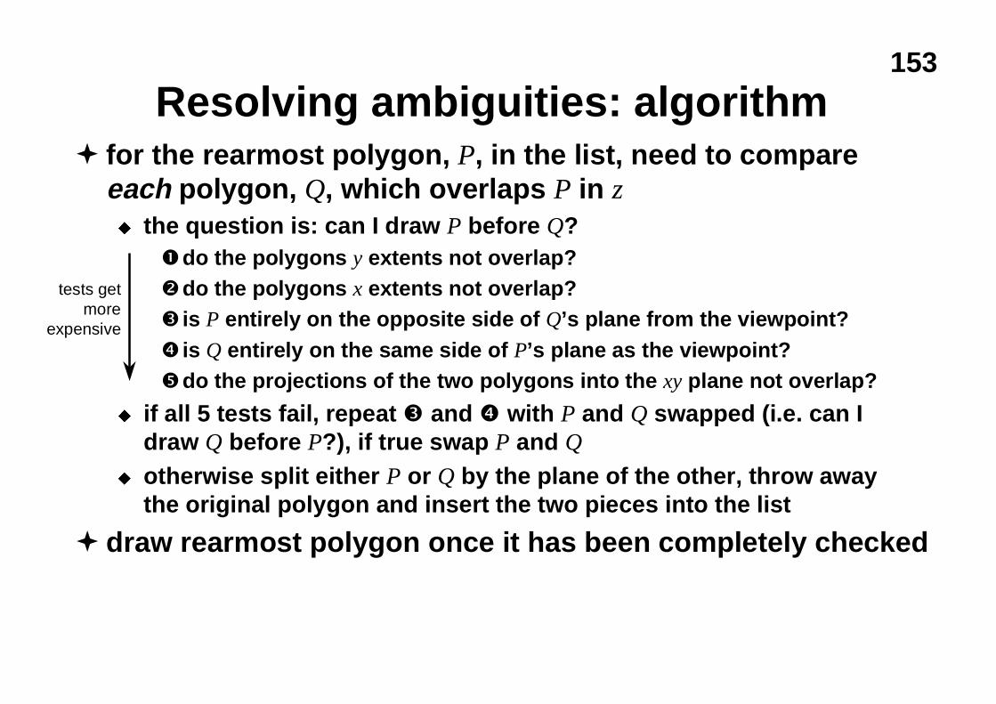
Resolving ambiguities: algorithm� for the rearmost polygon, P, in the list, need to compare

each polygon, Q, which overlaps P in zu the question is: can I draw P before Q?

èdo the polygons y extents not overlap?�do the polygons x extents not overlap?� is P entirely on the opposite side of Q’s plane from the viewpoint?� is Q entirely on the same side of P’s plane as the viewpoint?�do the projections of the two polygons into the xy plane not overlap?

u if all 5 tests fail, repeat � and � with P and Q swapped (i.e. can Idraw Q before P?), if true swap P and Q

u otherwise split either P or Q by the plane of the other, throw awaythe original polygon and insert the two pieces into the list

� draw rearmost polygon once it has been completely checked

tests getmore

expensive

154

Depth sort: comments

u the depth sort algorithm produces a list ofpolygons which can be scan-converted in 2D,backmost to frontmost, to produce the correctimage

u reasonably cheap for small number of polygons,becomes expensive for large numbers of polygons

u the ordering is only valid from one particularviewpoint

155

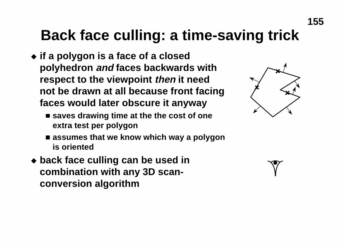
Back face culling: a time-saving tricku if a polygon is a face of a closed

polyhedron and faces backwards withrespect to the viewpoint then it neednot be drawn at all because front facingfaces would later obscure it anywayn saves drawing time at the the cost of one

extra test per polygonn assumes that we know which way a polygon

is oriented

u back face culling can be used incombination with any 3D scan-conversion algorithm

ã

ã

ã

156

Binary Space-Partitioning treesu BSP trees provide a way of quickly calculating the

correct depth order:n for a collection of static polygonsn from an arbitrary viewpoint

u the BSP tree trades off an initial time- and space-intensive pre-processing step against a linear displayalgorithm (O(N)) which is executed whenever a newviewpoint is specified

u the BSP tree allows you to easily determine thecorrect order in which to draw polygons by traversingthe tree in a simple way

157

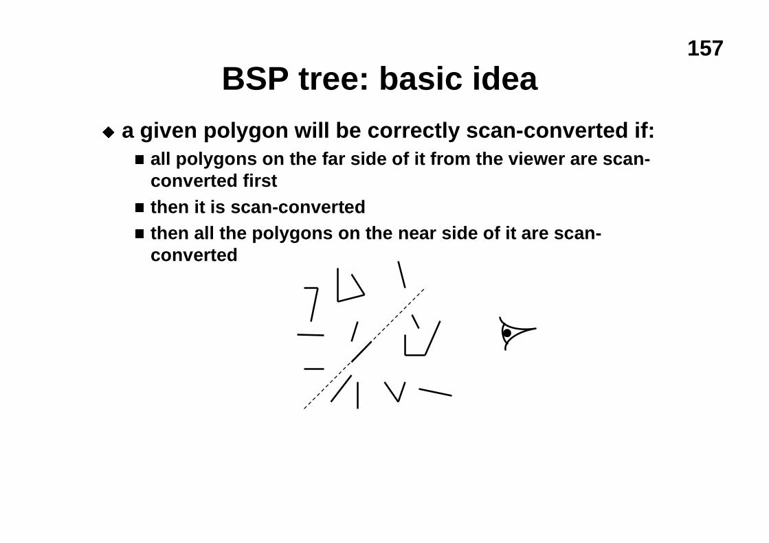
BSP tree: basic ideau a given polygon will be correctly scan-converted if:

n all polygons on the far side of it from the viewer are scan-converted first

n then it is scan-convertedn then all the polygons on the near side of it are scan-

converted

158

Making a BSP treeu given a set of polygons

n select an arbitrary polygon as the root of the treen divide all remaining polygons into two subsets:

v those in front of the selected polygon’s plane

v those behind the selected polygon’s plane

l any polygons through which the plane passes are splitinto two polygons and the two parts put into theappropriate subsets

n make two BSP trees, one from each of the two subsetsl these become the front and back subtrees of the root

159

Drawing a BSP treeu if the viewpoint is in front of the root’s polygon’s

plane then:n draw the BSP tree for the back child of the rootn draw the root’s polygonn draw the BSP tree for the front child of the root

u otherwise:n draw the BSP tree for the front child of the rootn draw the root’s polygonn draw the BSP tree for the back child of the root

160Scan-line algorithms

u instead of drawing one polygon at a time:modify the 2D polygon scan-conversion algorithm to handleall of the polygons at once

u the algorithm keeps a list of the active edges in all polygonsand proceeds one scan-line at a timen there is thus one large active edge list and one (even larger) edge list

l enormous memory requirements

u still fill in pixels between adjacent pairs of edges on thescan-line but:n need to be intelligent about which polygon is in front

and therefore what colours to put in the pixelsn every edge is used in two pairs:

one to the left and one to the right of it

161

z-buffer polygon scan conversion

�depth sort & BSP-tree methods involve cleversorting algorithms followed by the invocationof the standard 2D polygon scan conversionalgorithm

�by modifying the 2D scan conversionalgorithm we can remove the need to sort thepolygonsu makes hardware implementation easier

162

z-buffer basics

�store both colour and depth at each pixel�when scan converting a polygon:

u calculate the polygon’s depth at each pixelu if the polygon is closer than the current depth

stored at that pixeln then store both the polygon’s colour and depth at that

pixeln otherwise do nothing

163

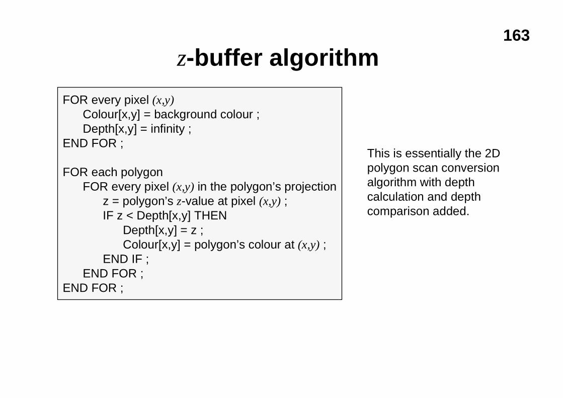
z-buffer algorithm

FOR every pixel (x,y)Colour[x,y] = background colour ;Depth[x,y] = infinity ;

END FOR ;

FOR each polygonFOR every pixel (x,y) in the polygon’s projection

z = polygon’s z-value at pixel (x,y) ;IF z < Depth[x,y] THEN

Depth[x,y] = z ;Colour[x,y] = polygon’s colour at (x,y) ;

END IF ;END FOR ;

END FOR ;

This is essentially the 2Dpolygon scan conversionalgorithm with depthcalculation and depthcomparison added.

164

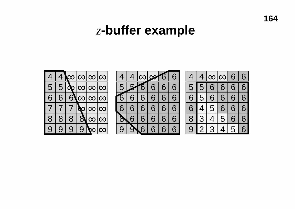
z-buffer example

9 9 9 9 ∞ ∞8 8 8 8 ∞ ∞7 7 7 ∞ ∞ ∞6 6 6 ∞ ∞ ∞5 5 ∞ ∞ ∞ ∞4 4 ∞ ∞ ∞ ∞

9 9 6 6 6 68 6 6 6 6 66 6 6 6 6 66 6 6 6 6 65 5 6 6 6 64 4 ∞ ∞ 6 6

9 2 3 4 5 68 3 4 5 6 66 4 5 6 6 66 5 6 6 6 65 5 6 6 6 64 4 ∞ ∞ 6 6

165

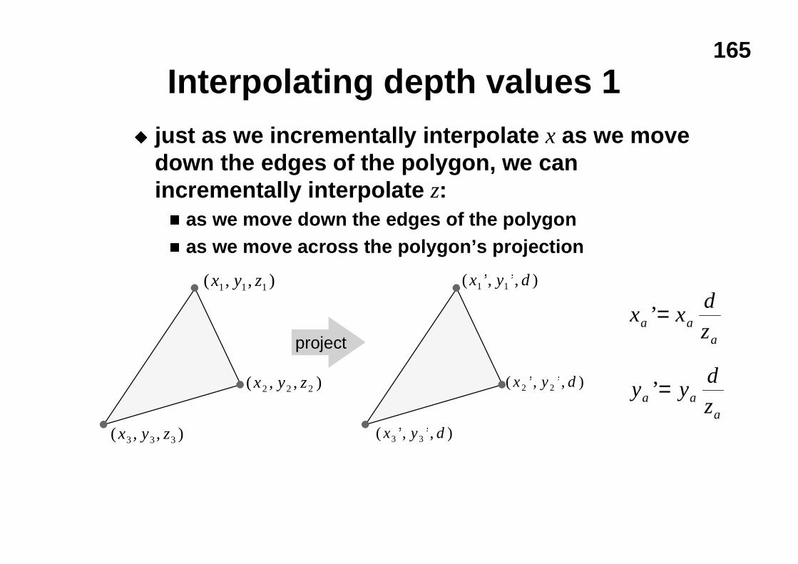
Interpolating depth values 1u just as we incrementally interpolate x as we move

down the edges of the polygon, we canincrementally interpolate z:n as we move down the edges of the polygonn as we move across the polygon’s projection

( , , )x y z1 1 1

( , , )x y z2 2 2

( , , )x y z3 3 3

( ’, ’, )x y d1 1

( ’, ’, )x y d2 2

( ’, ’, )x y d3 3

project

x xd

z

y yd

z

a aa

a aa

’

’

=

=

166

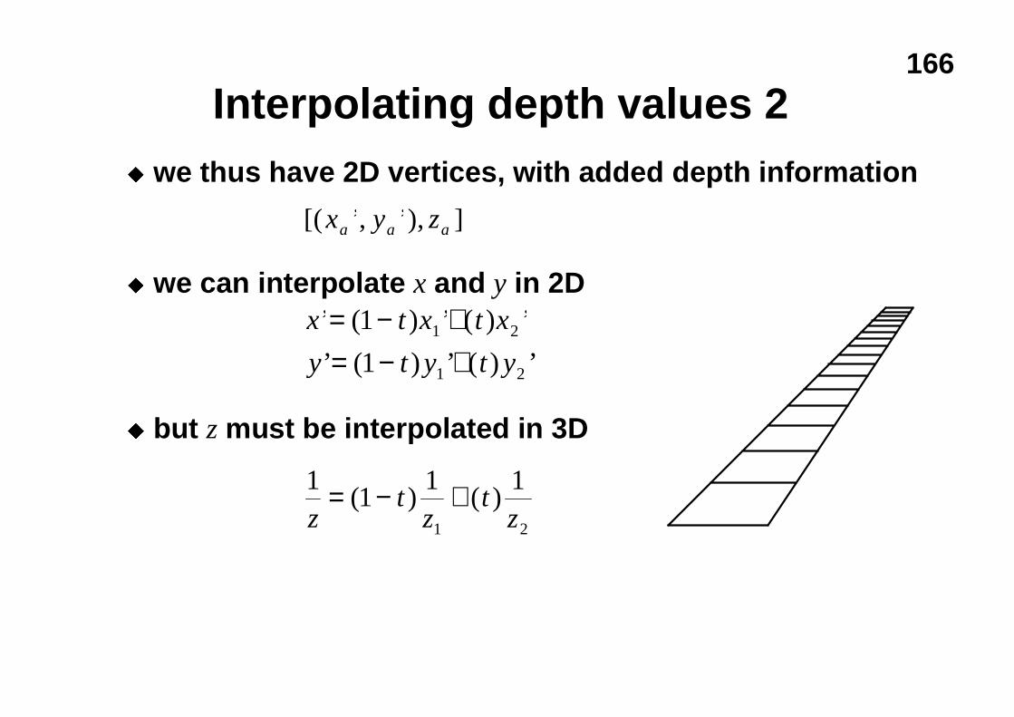
Interpolating depth values 2u we thus have 2D vertices, with added depth information

u we can interpolate x and y in 2D

u but z must be interpolated in 3D

[( ’, ’), ]x y za a a

x t x t x

y t y t y

’ ( ) ’ ( ) ’

’ ( ) ’ ( ) ’

= − += − +

1

11 2

1 2

11

1 1

1 2zt

zt

z= − +( ) ( )

167

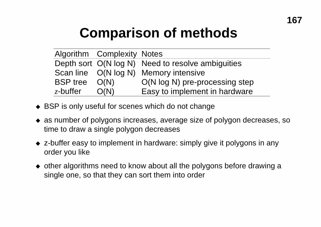
Comparison of methods

u BSP is only useful for scenes which do not change

u as number of polygons increases, average size of polygon decreases, sotime to draw a single polygon decreases

u z-buffer easy to implement in hardware: simply give it polygons in anyorder you like

u other algorithms need to know about all the polygons before drawing asingle one, so that they can sort them into order

Algorithm Complexity NotesDepth sort O(N log N) Need to resolve ambiguitiesScan line O(N log N) Memory intensiveBSP tree O(N) O(N log N) pre-processing stepz-buffer O(N) Easy to implement in hardware

168

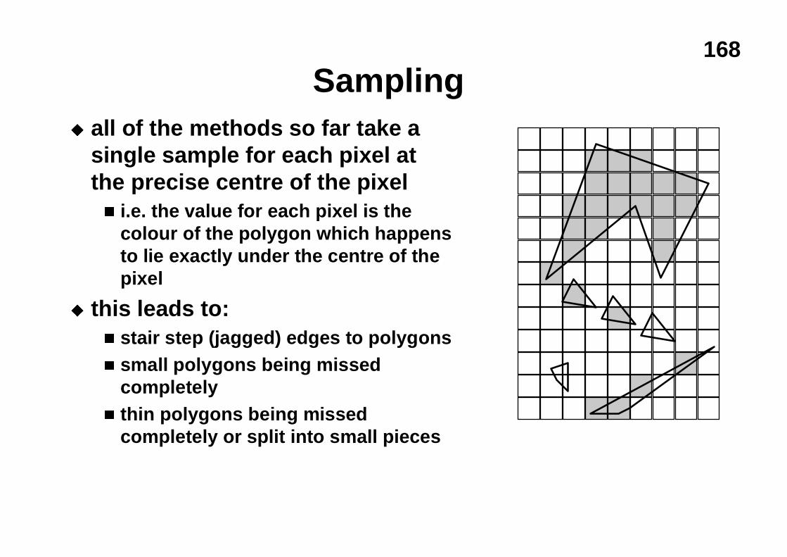
Samplingu all of the methods so far take a

single sample for each pixel atthe precise centre of the pixeln i.e. the value for each pixel is the

colour of the polygon which happensto lie exactly under the centre of thepixel

u this leads to:n stair step (jagged) edges to polygonsn small polygons being missed

completelyn thin polygons being missed

completely or split into small pieces

169

Anti-aliasingu these artefacts (and others) are jointly known as

aliasingu methods of ameliorating the effects of aliasing are

known as anti-aliasing

n in signal processing aliasing is a precisely defined technicalterm for a particular kind of artefact

n in computer graphics its meaning has expanded to includemost undesirable effects that can occur in the imagel this is because the same anti-aliasing techniques which

ameliorate true aliasing artefacts also ameliorate most of theother artefacts

170

Anti-aliasing method 1: area averagingu average the contributions of all polygons to

each pixeln e.g. assume pixels are square and we just want the

average colour in the squaren Ed Catmull developed an algorithm which does this:

l works a scan-line at a time

l clips all polygons to the scan-line

l determines the fragment of each polygon whichprojects to each pixel

l determines the amount of the pixel covered by thevisible part of each fragment

l pixel’s colour is a weighted sum of the visible parts

n expensive algorithm!

171

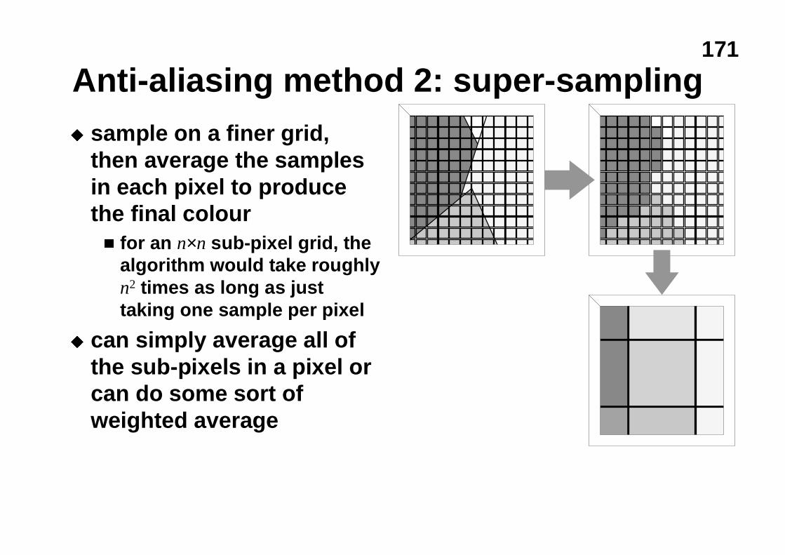
Anti-aliasing method 2: super-samplingu sample on a finer grid,

then average the samplesin each pixel to producethe final colourn for an n×n sub-pixel grid, the

algorithm would take roughlyn2 times as long as justtaking one sample per pixel

u can simply average all ofthe sub-pixels in a pixel orcan do some sort ofweighted average

172

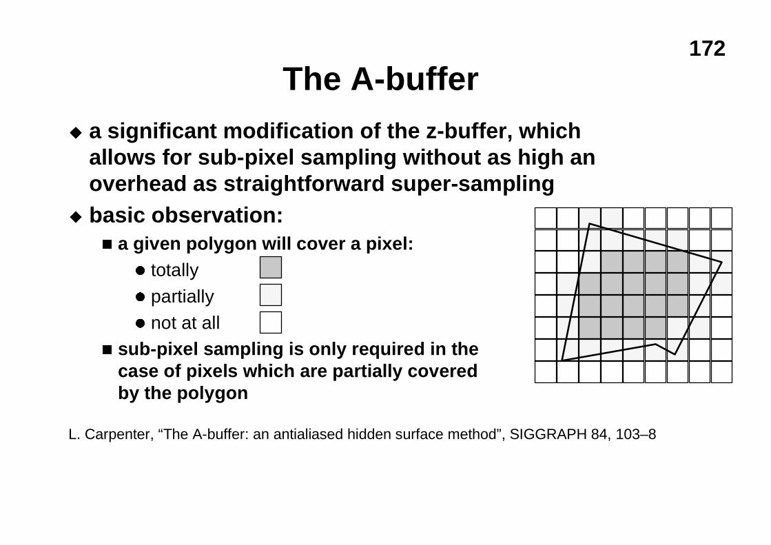
The A-bufferu a significant modification of the z-buffer, which

allows for sub-pixel sampling without as high anoverhead as straightforward super-sampling

u basic observation:n a given polygon will cover a pixel:

l totally

l partially

l not at alln sub-pixel sampling is only required in the

case of pixels which are partially coveredby the polygon

L. Carpenter, “The A-buffer: an antialiased hidden surface method”, SIGGRAPH 84, 103–8

173

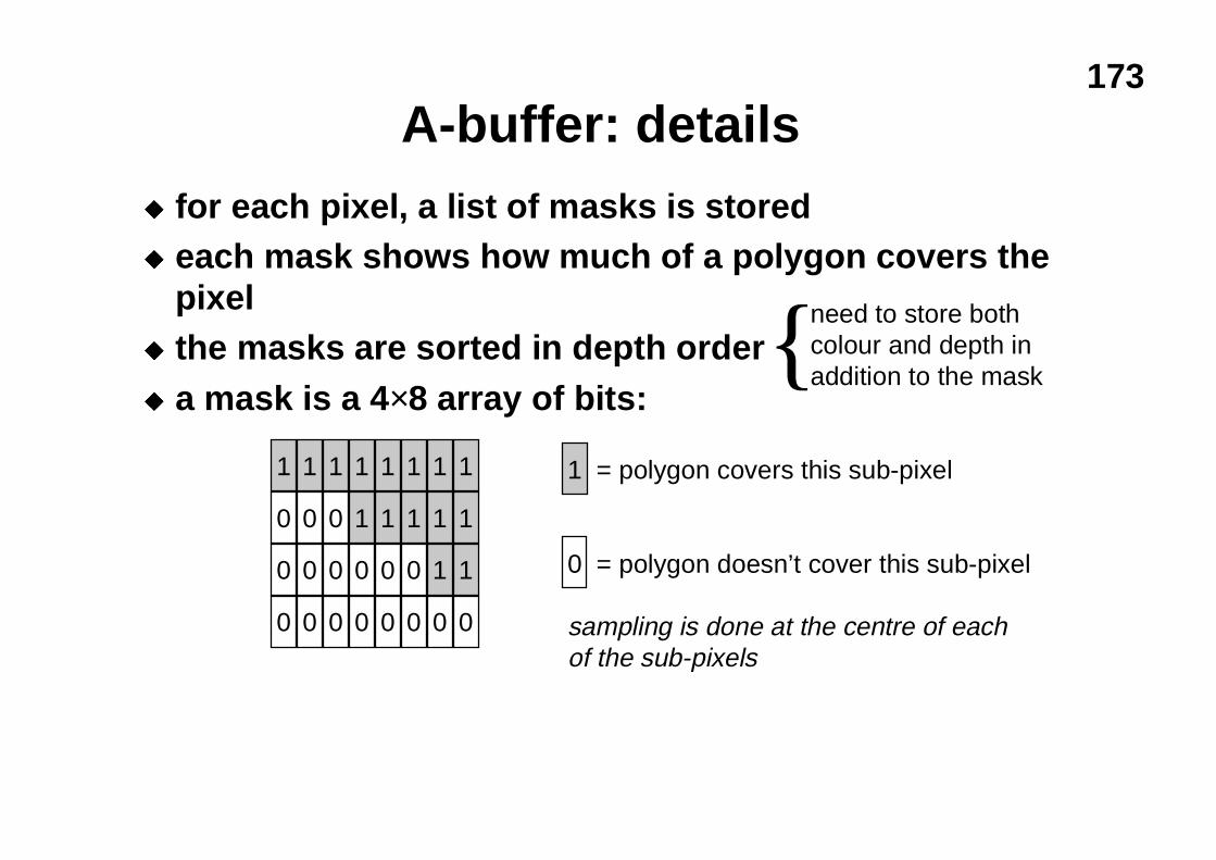
A-buffer: detailsu for each pixel, a list of masks is storedu each mask shows how much of a polygon covers the

pixelu the masks are sorted in depth orderu a mask is a 4×8 array of bits:

1 1 1 1 1 1 1 1

0 0 0 1 1 1 1 1

0 0 0 0 0 0 1 1

0 0 0 0 0 0 0 0

1 = polygon covers this sub-pixel

0 = polygon doesn’t cover this sub-pixel

sampling is done at the centre of eachof the sub-pixels

need to store bothcolour and depth inaddition to the mask{

174

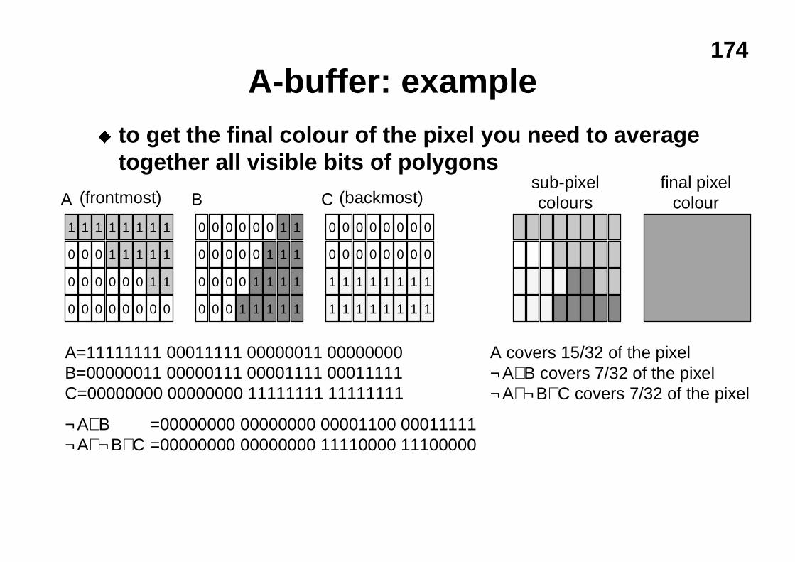
A-buffer: exampleu to get the final colour of the pixel you need to average

together all visible bits of polygons

1 1 1 1 1 1 1 1

0 0 0 1 1 1 1 1

0 0 0 0 0 0 1 1

0 0 0 0 0 0 0 0

0 0 0 0 0 0 1 1

0 0 0 0 0 1 1 1

0 0 0 0 1 1 1 1

0 0 0 1 1 1 1 1 1 1 1 1 1 1 1 1

0 0 0 0 0 0 0 0

1 1 1 1 1 1 1 1

0 0 0 0 0 0 0 0

sub-pixelcolours

final pixelcolour(frontmost) (backmost)

A=11111111 00011111 00000011 00000000B=00000011 00000111 00001111 00011111C=00000000 00000000 11111111 11111111

¬A∧B =00000000 00000000 00001100 00011111¬A∧¬B∧C =00000000 00000000 11110000 11100000

A covers 15/32 of the pixel¬A∧B covers 7/32 of the pixel¬A∧¬B∧C covers 7/32 of the pixel

A B C

175

Making the A-buffer more efficientu if a polygon totally covers a pixel then:

n do not need to calculate a mask, because the mask is all 1sn all masks currently in the list which are behind this polygon

can be discardedn any subsequent polygons which are behind this polygon can

be immediately discounted (without calculating a mask)

u in most scenes, therefore, the majority of pixels willhave only a single entry in their list of masks

u the polygon scan-conversion algorithm can bestructured so that it is immediately obvious whether apixel is totally or partially within a polygon

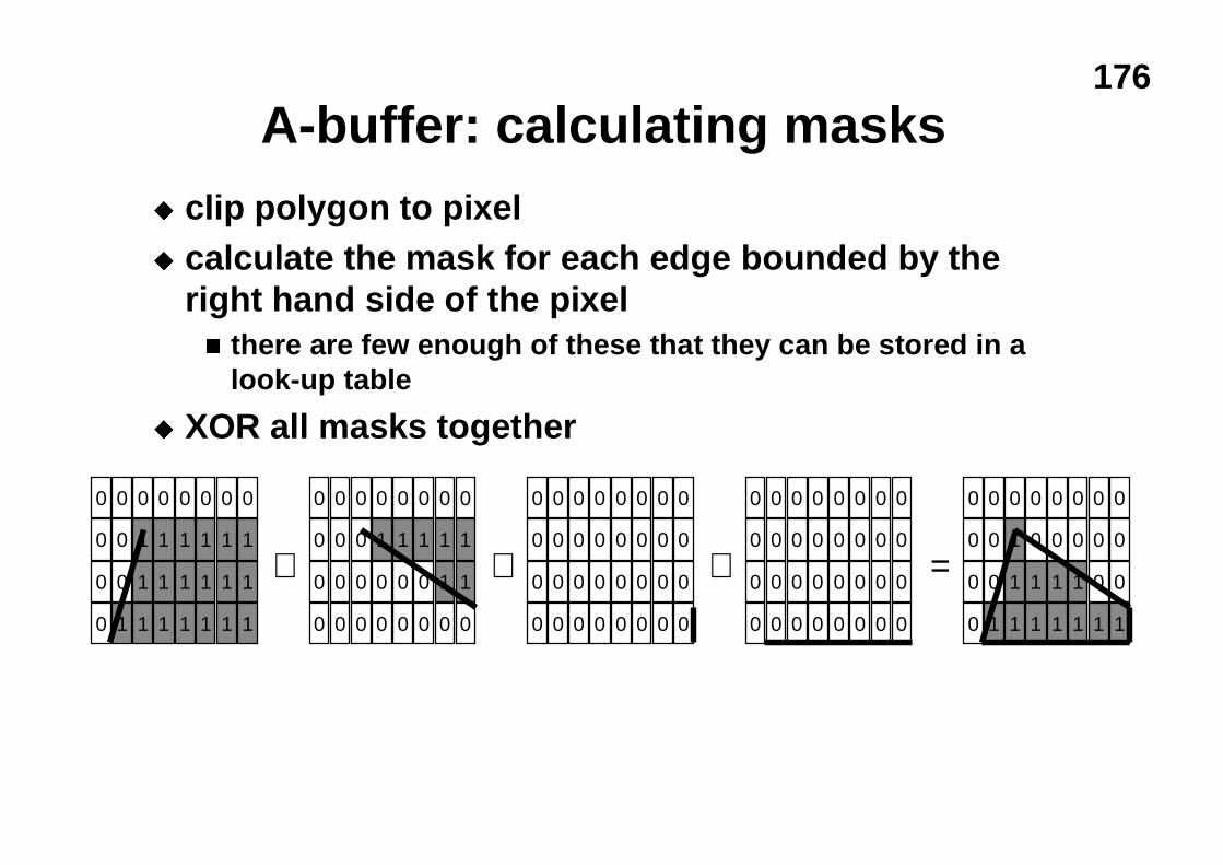
176

A-buffer: calculating masksu clip polygon to pixelu calculate the mask for each edge bounded by the

right hand side of the pixeln there are few enough of these that they can be stored in a

look-up table

u XOR all masks together

0 0 0 0 0 0 0 0

0 0 1 0 0 0 0 0

0 0 1 1 1 1 0 0

0 1 1 1 1 1 1 1

0 0 0 0 0 0 0 0

0 0 0 0 0 0 0 0

0 0 0 0 0 0 0 0

0 0 0 0 0 0 0 0

0 0 0 0 0 0 0 0

0 0 0 0 0 0 0 0

0 0 0 0 0 0 0 0

0 0 0 0 0 0 0 0

0 0 0 0 0 0 0 0

0 0 1 1 1 1 1 1

0 0 1 1 1 1 1 1

0 1 1 1 1 1 1 1

0 0 0 0 0 0 0 0

0 0 0 1 1 1 1 1

0 0 0 0 0 0 1 1

0 0 0 0 0 0 0 0

⊕ ⊕ ⊕ =

177

A-buffer: commentsu the A-buffer algorithm essentially adds anti-aliasing to

the z-buffer algorithm in an efficient way

u most operations on masks are AND, OR, NOT, XORn very efficient boolean operations

u why 4×8?n algorithm originally implemented on a machine with 32-bit

registers (VAX 11/780)n on a 64-bit register machine, 8×8 seems more sensible

u what does the A stand for in A-buffer?n anti-aliased, area averaged, accumulator

178

A-buffer: extensionsu as presented the algorithm assumes that a mask has

a constant depth (z value)n can modify the algorithm and perform approximate

intersection between polygons

u can save memory by combining fragments whichstart life in the same primitiven e.g. two triangles that are part of the decomposition of a

Bezier patch

u can extend to allow transparent objects

179

Illumination & shadingu until now we have assumed that each polygon is a

uniform colour and have not thought about how thatcolour is determined

u things look more realistic if there is some sort ofillumination in the scene

u we therefore need a mechanism of determining thecolour of a polygon based on its surface propertiesand the positions of the lights

u we will, as a consequence, need to find ways toshade polygons which do not have a uniform colour

180

Illumination & shading (continued)u in the real world every light source emits millions of

photons every secondu these photons bounce off objects, pass through

objects, and are absorbed by objectsu a tiny proportion of these photons enter your eyes

allowing you to see the objects

u tracing the paths of all these photons is not an efficientway of calculating the shading on the polygons in yourscene

181

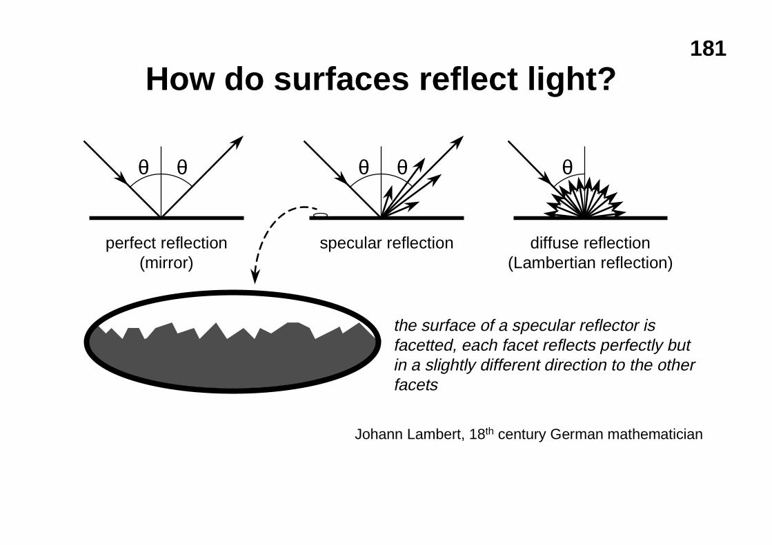
How do surfaces reflect light?

θ θ θ θ θ

perfect reflection(mirror)

specular reflection diffuse reflection(Lambertian reflection)

Johann Lambert, 18th century German mathematician

the surface of a specular reflector isfacetted, each facet reflects perfectly butin a slightly different direction to the otherfacets

182

Comments on reflectionu the surface can absorb some wavelengths of light

n e.g. shiny gold or shiny copper

u specular reflection has “interesting” properties atglancing angles owing to occlusion of micro-facets byone another

u plastics are good examples of surfaces with:n specular reflection in the light’s colourn diffuse reflection in the plastic’s colour

183

Calculating the shading of a polygonu gross assumptions:

n there is only diffuse (Lambertian) reflectionn all light falling on a polygon comes directly from a light source

l there is no interaction between polygons

n no polygon casts shadows on any otherl so can treat each polygon as if it were the only polygon in the scene

n light sources are considered to be infinitely distant from thepolygonl the vector to the light is the same across the whole polygon

u observation:n the colour of a flat polygon will be uniform across its surface,

dependent only on the colour & position of the polygon and thecolour & position of the light sources

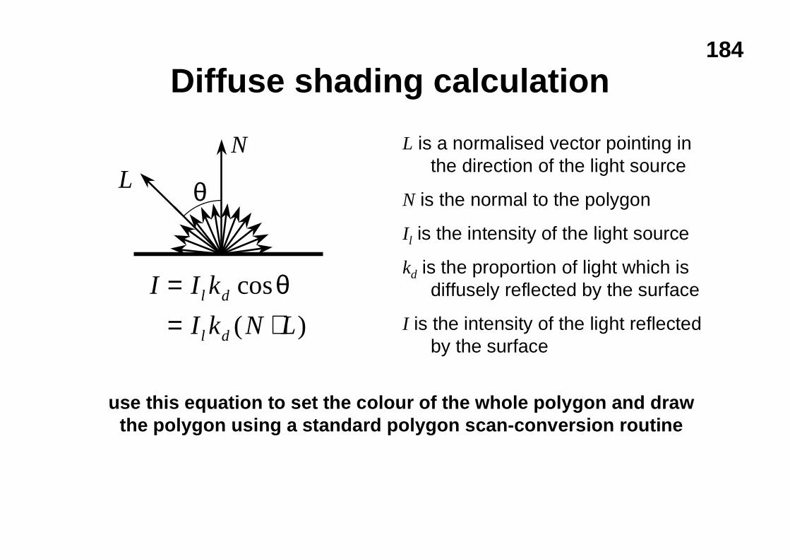
184

Diffuse shading calculation

L is a normalised vector pointing inthe direction of the light source

N is the normal to the polygon

Il is the intensity of the light source

kd is the proportion of light which isdiffusely reflected by the surface

I is the intensity of the light reflectedby the surface

θL

N

I I k

I k N Ll d

l d

== ⋅

cos

( )

θ

use this equation to set the colour of the whole polygon and drawthe polygon using a standard polygon scan-conversion routine

185

Diffuse shading: commentsu can have different Il and different kd for different

wavelengths (colours)u watch out for cosθ < 0

n implies that the light is behind the polygon and so it cannotilluminate this side of the polygon

u do you use one-sided or two-sided polygons?n one sided: only the side in the direction of the normal vector

can be illuminatedl if cosθ < 0 then both sides are black

n two sided: the sign of cosθ determines which side of thepolygon is illuminatedl need to invert the sign of the intensity for the back side

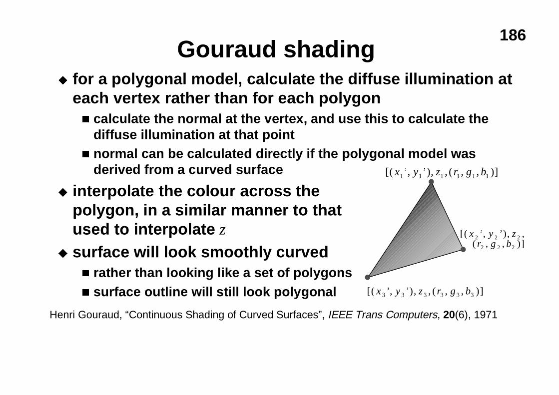
186Gouraud shading

u for a polygonal model, calculate the diffuse illumination ateach vertex rather than for each polygonn calculate the normal at the vertex, and use this to calculate the

diffuse illumination at that pointn normal can be calculated directly if the polygonal model was

derived from a curved surface

u interpolate the colour across thepolygon, in a similar manner to thatused to interpolate z

u surface will look smoothly curvedn rather than looking like a set of polygonsn surface outline will still look polygonal

[( ’, ’), , ( , , )]x y z r g b1 1 1 1 1 1

[( ’, ’), ,( , , )]

x y zr g b

2 2 2

2 2 2

[( ’, ’), , ( , , )]x y z r g b3 3 3 3 3 3

Henri Gouraud, “Continuous Shading of Curved Surfaces”, IEEE Trans Computers, 20(6), 1971

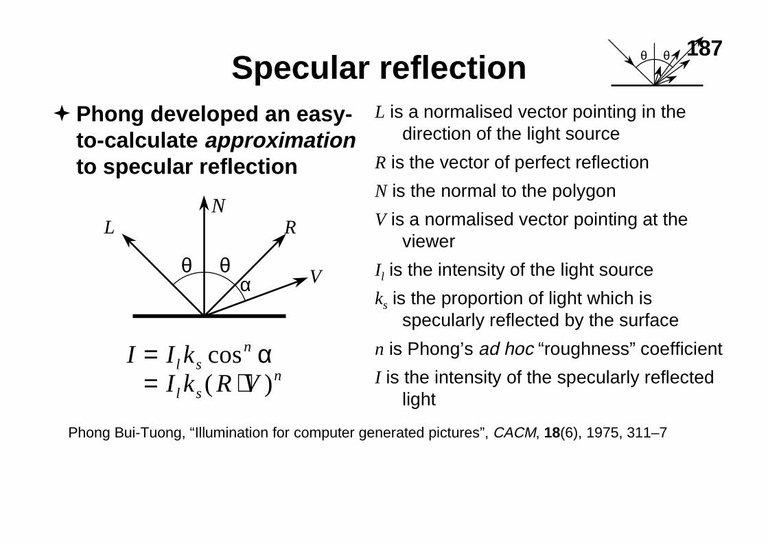
187Specular reflection

�Phong developed an easy-to-calculate approximationto specular reflection

θ θα

NR

V

L

θ θ

L is a normalised vector pointing in thedirection of the light source

R is the vector of perfect reflection

N is the normal to the polygon

V is a normalised vector pointing at theviewer

Il is the intensity of the light source

ks is the proportion of light which isspecularly reflected by the surface

n is Phong’s ad hoc “roughness” coefficient

I is the intensity of the specularly reflectedlight

I I kI k R V

l sn

l sn

== ⋅

cos( )

α

Phong Bui-Tuong, “Illumination for computer generated pictures”, CACM, 18(6), 1975, 311–7

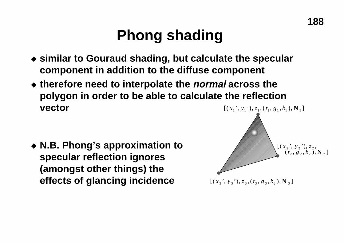
188

Phong shadingu similar to Gouraud shading, but calculate the specular

component in addition to the diffuse componentu therefore need to interpolate the normal across the

polygon in order to be able to calculate the reflectionvector

u N.B. Phong’s approximation tospecular reflection ignores(amongst other things) theeffects of glancing incidence

[( ’, ’), , ( , , ), ]x y z r g b1 1 1 1 1 1 1N

[( ’, ’) , ,( , , ), ]

x y zr g b

2 2 2

2 2 2 2N

[ ( ’, ’) , , ( , , ) , ]x y z r g b3 3 3 3 3 3 3N

189

The gross assumptions revisitedu only diffuse reflection

n now have a method of approximating specular reflection

u no shadowsn need to do ray tracing to get shadows

u lights at infinityn can add local lights at the expense of more calculation

l need to interpolate the L vector

u no interaction between surfacesn cheat!

l assume that all light reflected off all other surfaces onto a givenpolygon can be amalgamated into a single constant term: “ambientillumination”, add this onto the diffuse and specular illumination

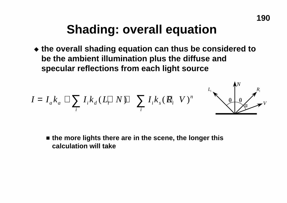
190

Shading: overall equationu the overall shading equation can thus be considered to

be the ambient illumination plus the diffuse andspecular reflections from each light source

n the more lights there are in the scene, the longer thiscalculation will take

θ θα

NRi

V

Li

I I k I k L N I k R Va a i d i i s in

ii

= + ⋅ + ⋅∑∑ ( ) ( )

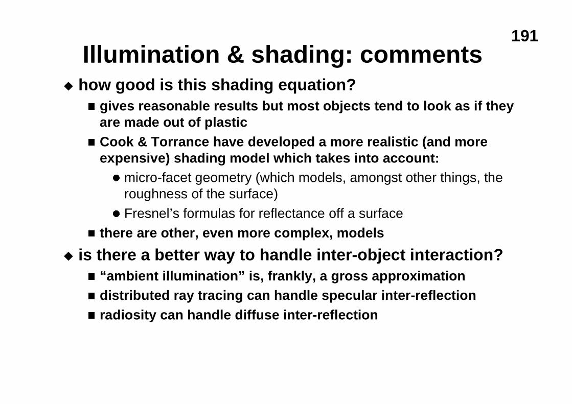
191Illumination & shading: comments

u how good is this shading equation?n gives reasonable results but most objects tend to look as if they

are made out of plasticn Cook & Torrance have developed a more realistic (and more

expensive) shading model which takes into account:l micro-facet geometry (which models, amongst other things, the

roughness of the surface)

l Fresnel’s formulas for reflectance off a surface

n there are other, even more complex, models

u is there a better way to handle inter-object interaction?n “ambient illumination” is, frankly, a gross approximationn distributed ray tracing can handle specular inter-reflectionn radiosity can handle diffuse inter-reflection

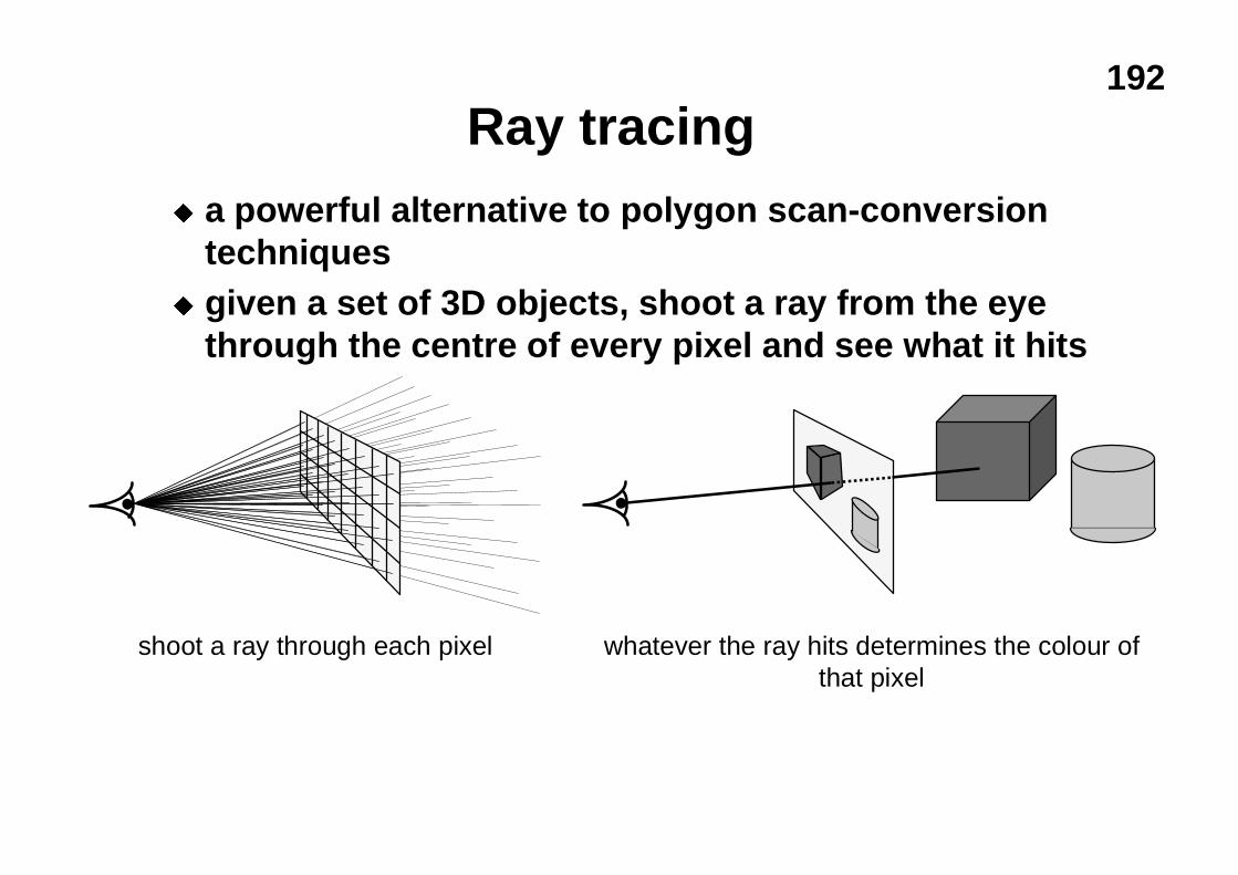
192

Ray tracingu a powerful alternative to polygon scan-conversion

techniquesu given a set of 3D objects, shoot a ray from the eye

through the centre of every pixel and see what it hits

shoot a ray through each pixel whatever the ray hits determines the colour ofthat pixel

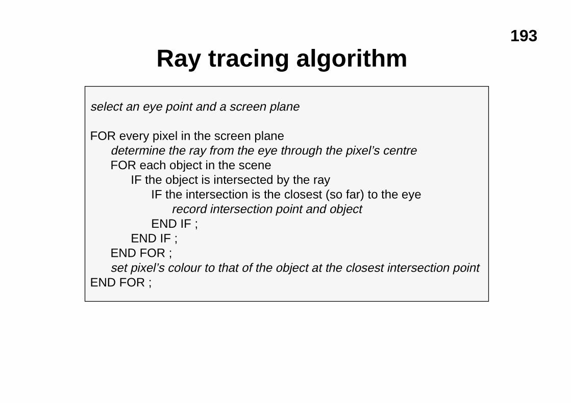
193

Ray tracing algorithm

select an eye point and a screen plane

FOR every pixel in the screen planedetermine the ray from the eye through the pixel’s centreFOR each object in the scene

IF the object is intersected by the rayIF the intersection is the closest (so far) to the eye

record intersection point and objectEND IF ;

END IF ;END FOR ;set pixel’s colour to that of the object at the closest intersection point

END FOR ;

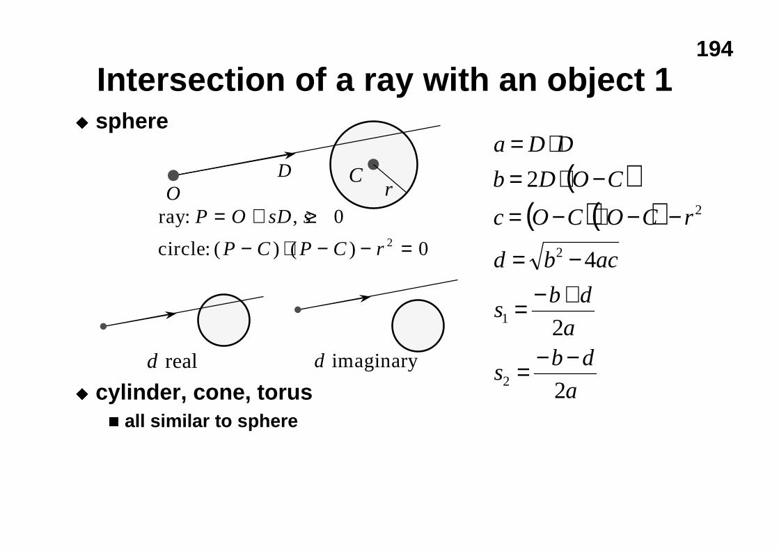
194

Intersection of a ray with an object 1u sphere

u cylinder, cone, torusn all similar to sphere

OD C

r ( )( ) ( )

a

dbs

a

dbs

acbd

rCOCOc

CODb

DDa

2

2

4

2

2

1

2

2

−−=

+−=

−=

−−⋅−=−⋅=

⋅=

d real d imaginary

ray

circle

: ,

: ( ) ( )

P O sD s

P C P C r

= + ≥− ⋅ − − =

0

02

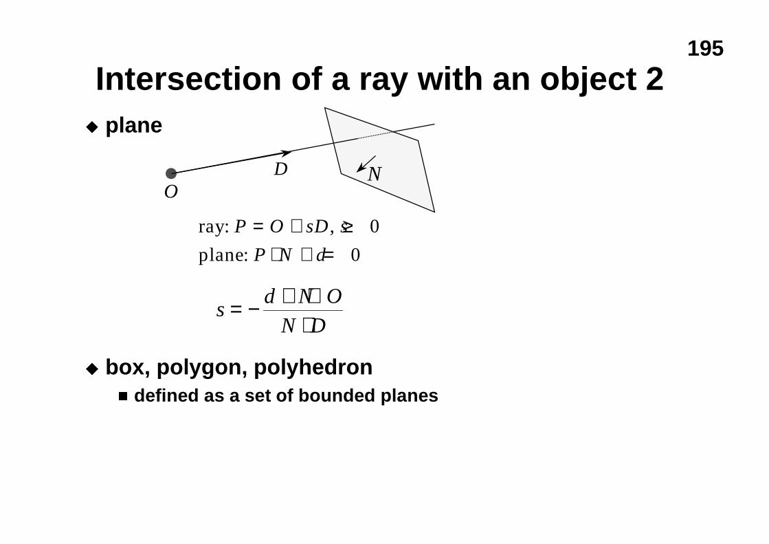
195

Intersection of a ray with an object 2u plane

u box, polygon, polyhedronn defined as a set of bounded planes

OD

ray

plane

: ,

:

P O sD s

P N d

= + ≥⋅ + =

0

0

N

sd N O

N D= − + ⋅

⋅

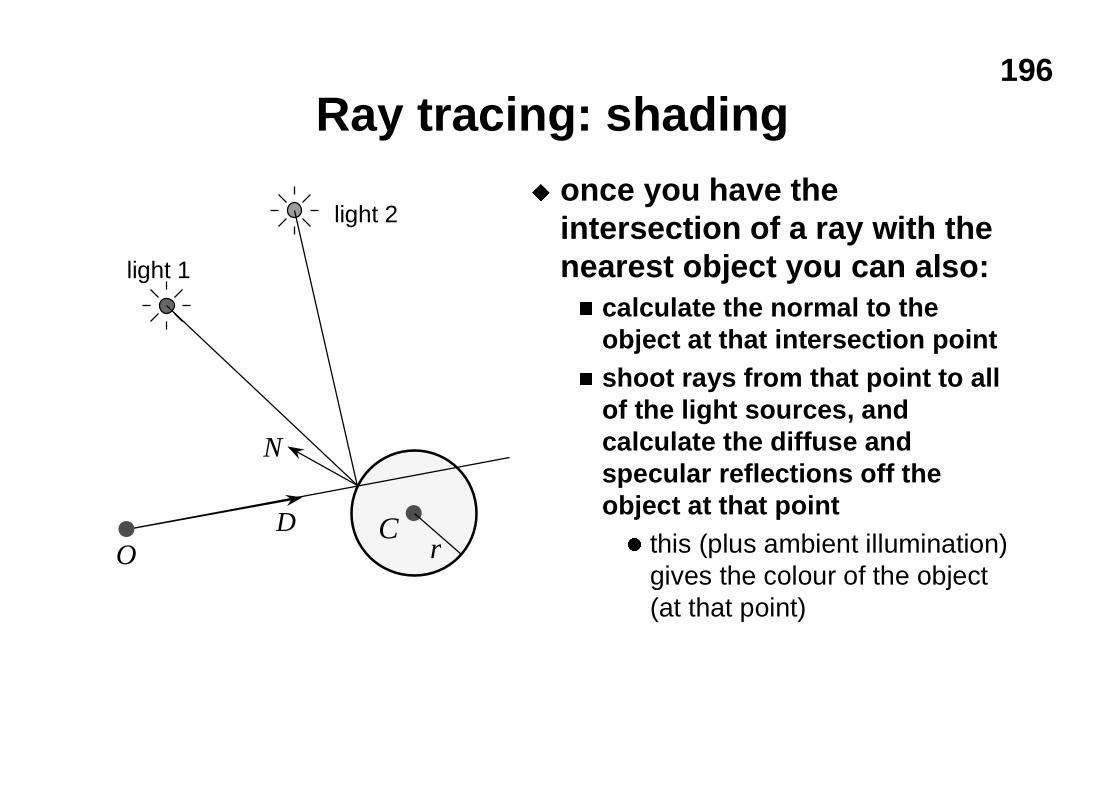
196

Ray tracing: shadingu once you have the

intersection of a ray with thenearest object you can also:n calculate the normal to the

object at that intersection pointn shoot rays from that point to all

of the light sources, andcalculate the diffuse andspecular reflections off theobject at that pointl this (plus ambient illumination)

gives the colour of the object(at that point)

OD C

r

N

light 1

light 2

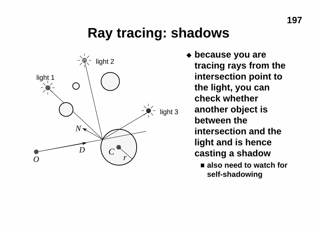
197

Ray tracing: shadowsu because you are

tracing rays from theintersection point tothe light, you cancheck whetheranother object isbetween theintersection and thelight and is hencecasting a shadown also need to watch for

self-shadowing

OD C

r

N

light 1

light 2

light 3

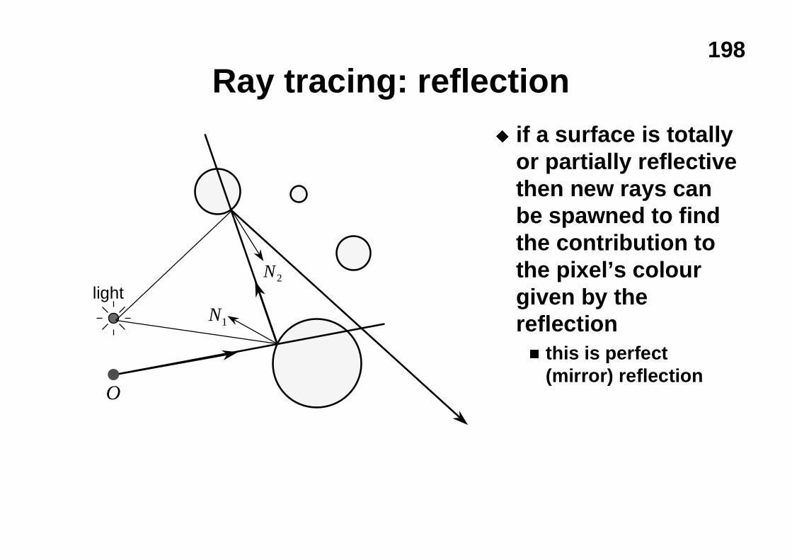
198

Ray tracing: reflectionu if a surface is totally

or partially reflectivethen new rays canbe spawned to findthe contribution tothe pixel’s colourgiven by thereflectionn this is perfect

(mirror) reflectionO

N1

lightN2

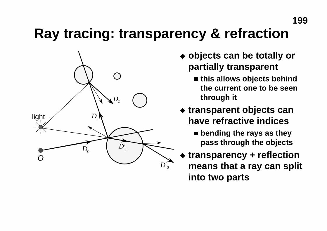
199

Ray tracing: transparency & refractionu objects can be totally or

partially transparentn this allows objects behind

the current one to be seenthrough it

u transparent objects canhave refractive indicesn bending the rays as they

pass through the objects

u transparency + reflectionmeans that a ray can splitinto two parts

O

light

D0

D1

D’1

D’2

D2

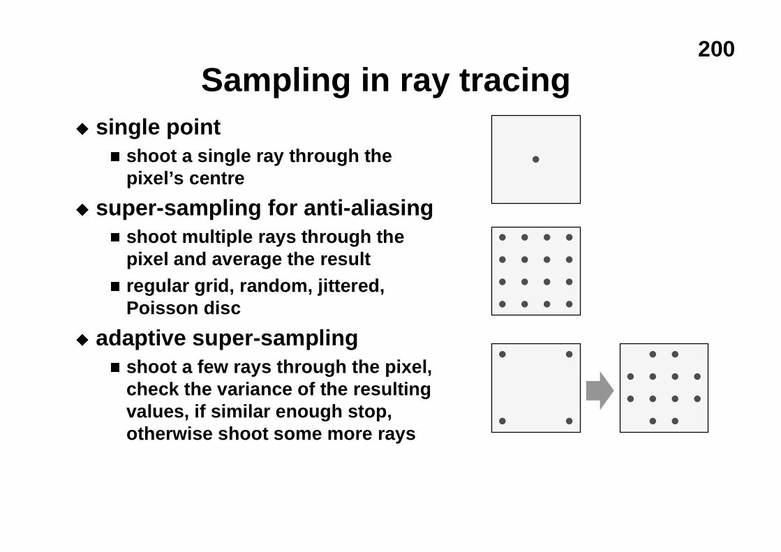
200

Sampling in ray tracingu single point

n shoot a single ray through thepixel’s centre

u super-sampling for anti-aliasingn shoot multiple rays through the

pixel and average the resultn regular grid, random, jittered,

Poisson disc

u adaptive super-samplingn shoot a few rays through the pixel,

check the variance of the resultingvalues, if similar enough stop,otherwise shoot some more rays

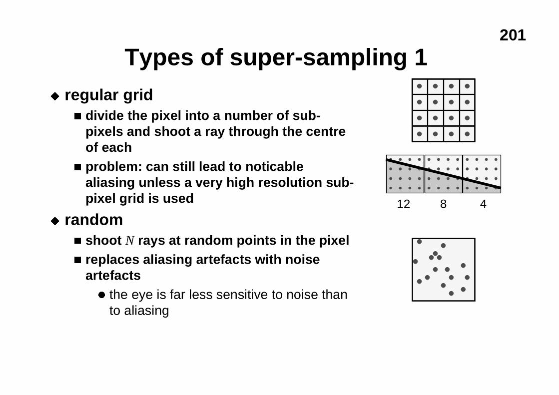
201

Types of super-sampling 1u regular grid

n divide the pixel into a number of sub-pixels and shoot a ray through the centreof each

n problem: can still lead to noticablealiasing unless a very high resolution sub-pixel grid is used

u randomn shoot N rays at random points in the pixeln replaces aliasing artefacts with noise

artefactsl the eye is far less sensitive to noise than

to aliasing

12 8 4

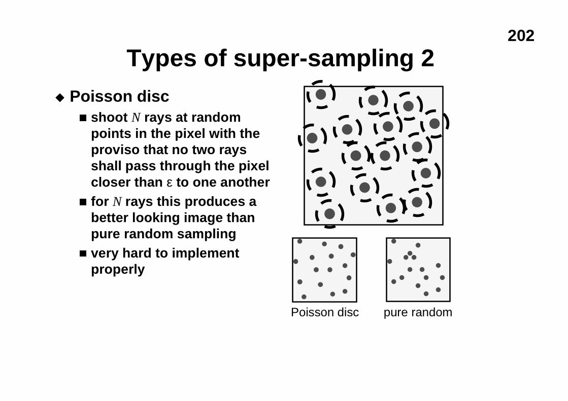
202

Types of super-sampling 2u Poisson disc

n shoot N rays at randompoints in the pixel with theproviso that no two raysshall pass through the pixelcloser than ε to one another

n for N rays this produces abetter looking image thanpure random sampling

n very hard to implementproperly

Poisson disc pure random

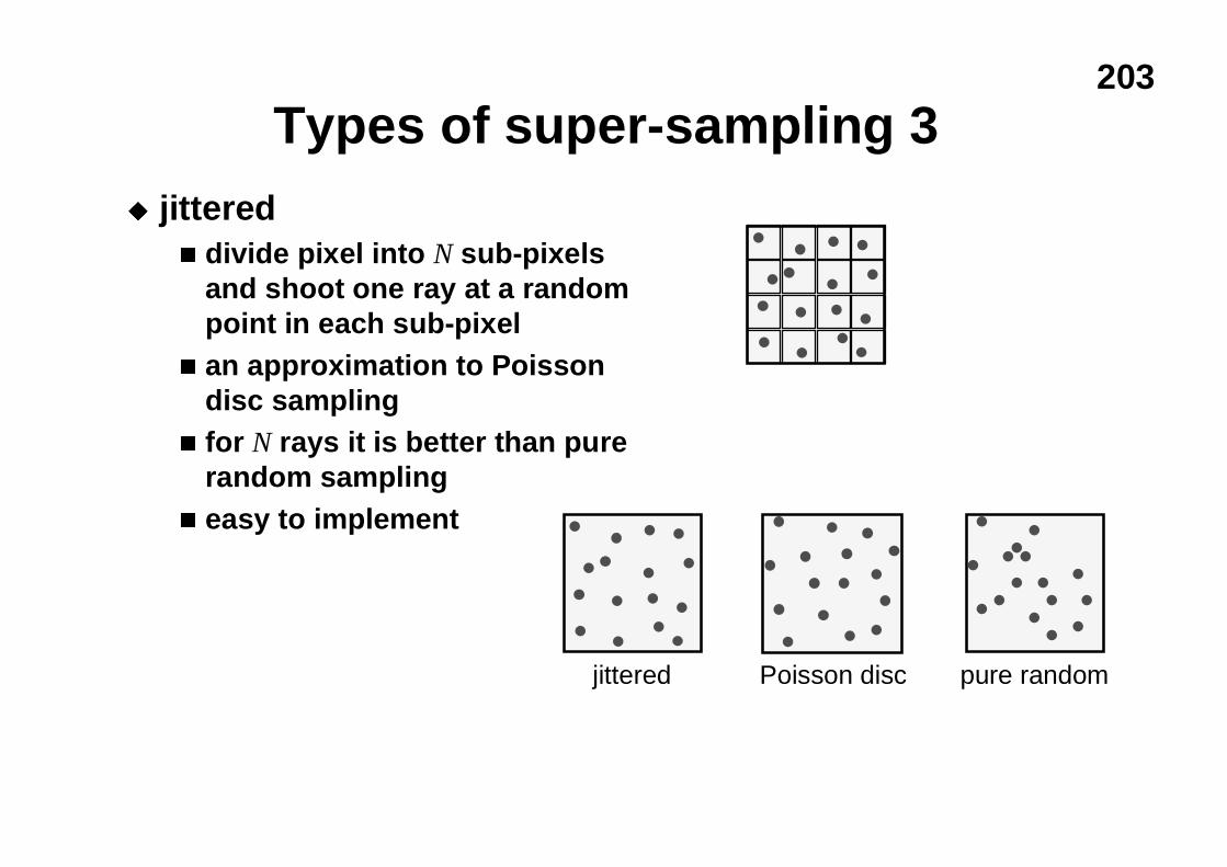
203

Types of super-sampling 3u jittered

n divide pixel into N sub-pixelsand shoot one ray at a randompoint in each sub-pixel

n an approximation to Poissondisc sampling

n for N rays it is better than purerandom sampling

n easy to implement

jittered pure randomPoisson disc

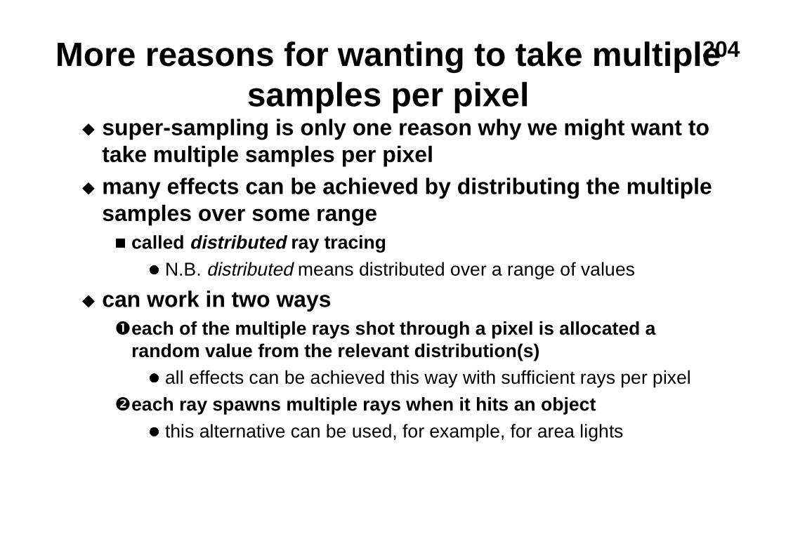
204More reasons for wanting to take multiplesamples per pixel

u super-sampling is only one reason why we might want totake multiple samples per pixel

u many effects can be achieved by distributing the multiplesamples over some rangen called distributed ray tracing

l N.B. distributed means distributed over a range of values

u can work in two waysèeach of the multiple rays shot through a pixel is allocated a

random value from the relevant distribution(s)l all effects can be achieved this way with sufficient rays per pixel

�each ray spawns multiple rays when it hits an objectl this alternative can be used, for example, for area lights

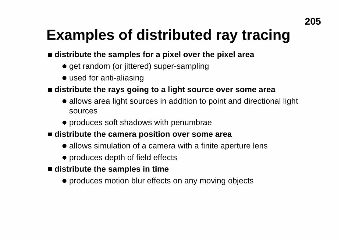
205

Examples of distributed ray tracingn distribute the samples for a pixel over the pixel area

l get random (or jittered) super-sampling

l used for anti-aliasing

n distribute the rays going to a light source over some areal allows area light sources in addition to point and directional light

sources

l produces soft shadows with penumbrae

n distribute the camera position over some areal allows simulation of a camera with a finite aperture lens

l produces depth of field effectsn distribute the samples in time

l produces motion blur effects on any moving objects

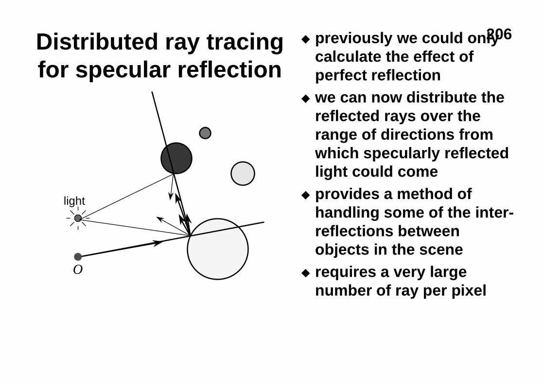
206Distributed ray tracingfor specular reflection

u previously we could onlycalculate the effect ofperfect reflection

u we can now distribute thereflected rays over therange of directions fromwhich specularly reflectedlight could come

u provides a method ofhandling some of the inter-reflections betweenobjects in the scene

u requires a very largenumber of ray per pixel

O

light

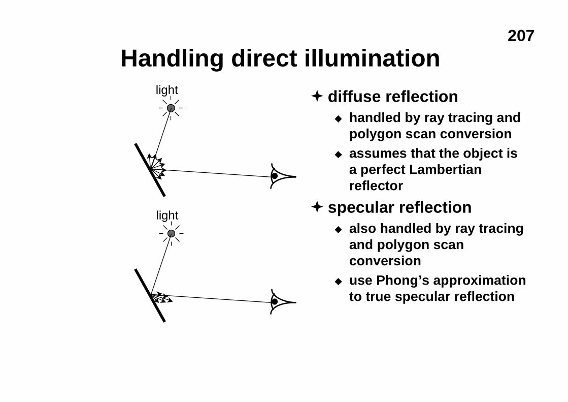
207

Handling direct illumination

light

light � diffuse reflectionu handled by ray tracing and

polygon scan conversionu assumes that the object is

a perfect Lambertianreflector

� specular reflectionu also handled by ray tracing

and polygon scanconversion

u use Phong’s approximationto true specular reflection

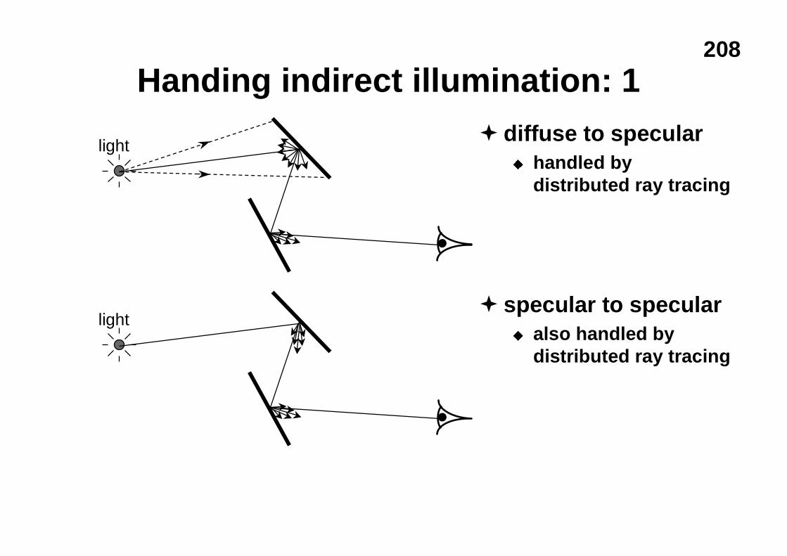
208

Handing indirect illumination: 1

light

light

� diffuse to specularu handled by

distributed ray tracing

� specular to specularu also handled by

distributed ray tracing

209

Handing indirect illumination: 2

light

light

� diffuse to diffuseu handled by radiosity

n covered in the Part IIAdvanced Graphicscourse

� specular to diffuseu handled by no usable

algorithmu some research work

has been done on thisbut uses enormousamounts of CPU time

210

Hybrid algorithms

�polygon scan conversion and ray tracing arethe two principal 3D rendering mechanismsu each has its advantages

n polygon scan conversion is fastern ray tracing produces more realistic looking results

�hybrid algorithms existu these generally use the speed of polygon scan

conversion for most of the work and use raytracing only to achieve particular special effects

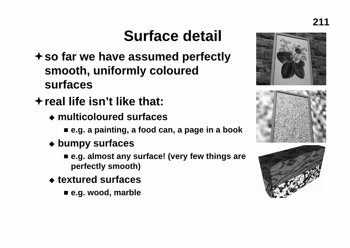
211

Surface detail�so far we have assumed perfectly

smooth, uniformly colouredsurfaces

�real life isn’t like that:u multicoloured surfaces

n e.g. a painting, a food can, a page in a book

u bumpy surfacesn e.g. almost any surface! (very few things are

perfectly smooth)

u textured surfacesn e.g. wood, marble

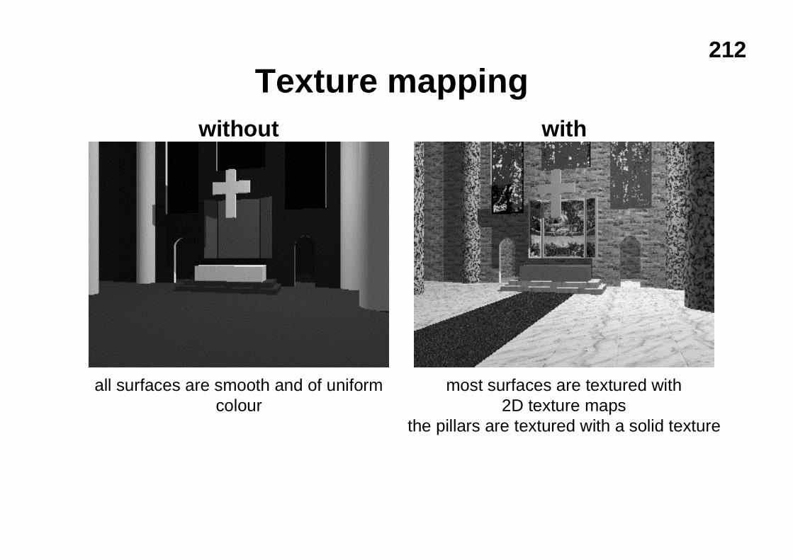
212

Texture mapping

all surfaces are smooth and of uniformcolour

most surfaces are textured with2D texture maps

the pillars are textured with a solid texture

without with

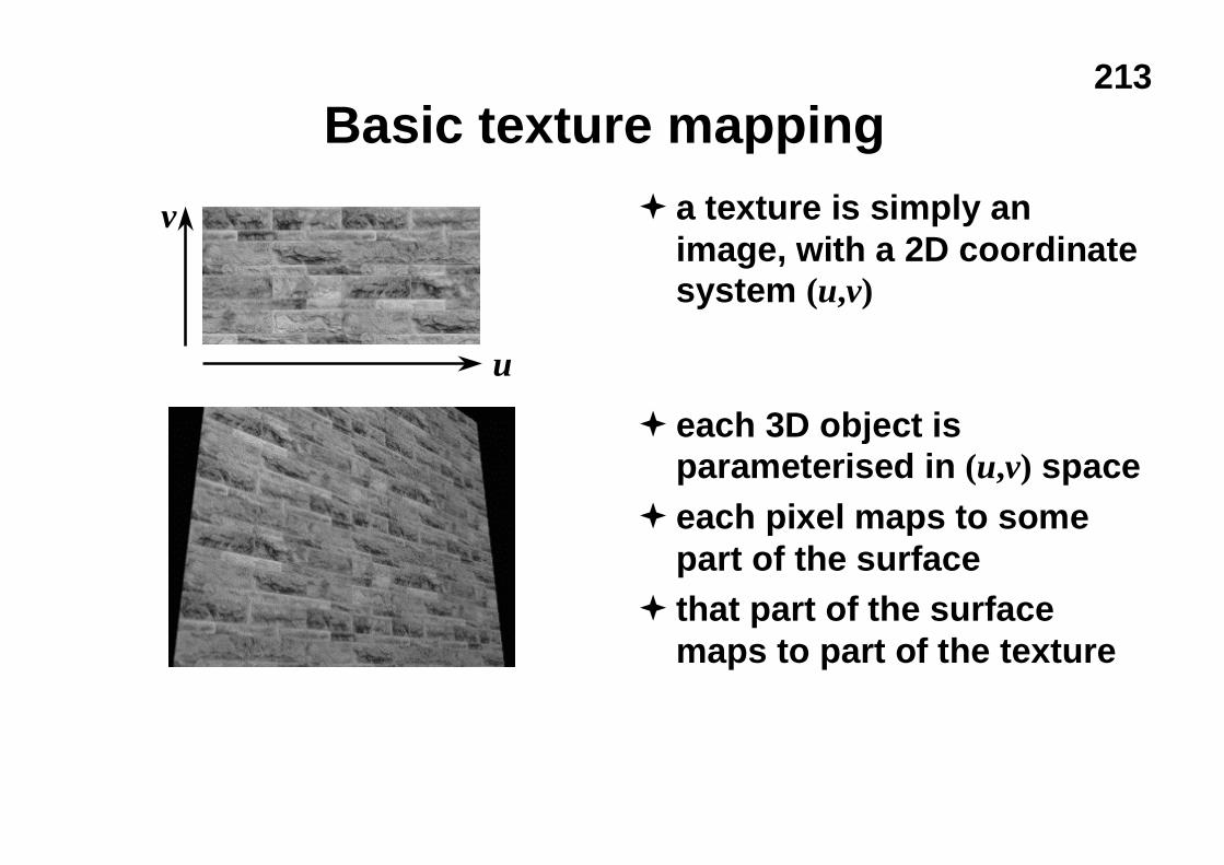
213

Basic texture mapping� a texture is simply an

image, with a 2D coordinatesystem (u,v)

� each 3D object isparameterised in (u,v) space

� each pixel maps to somepart of the surface

� that part of the surfacemaps to part of the texture

u

v

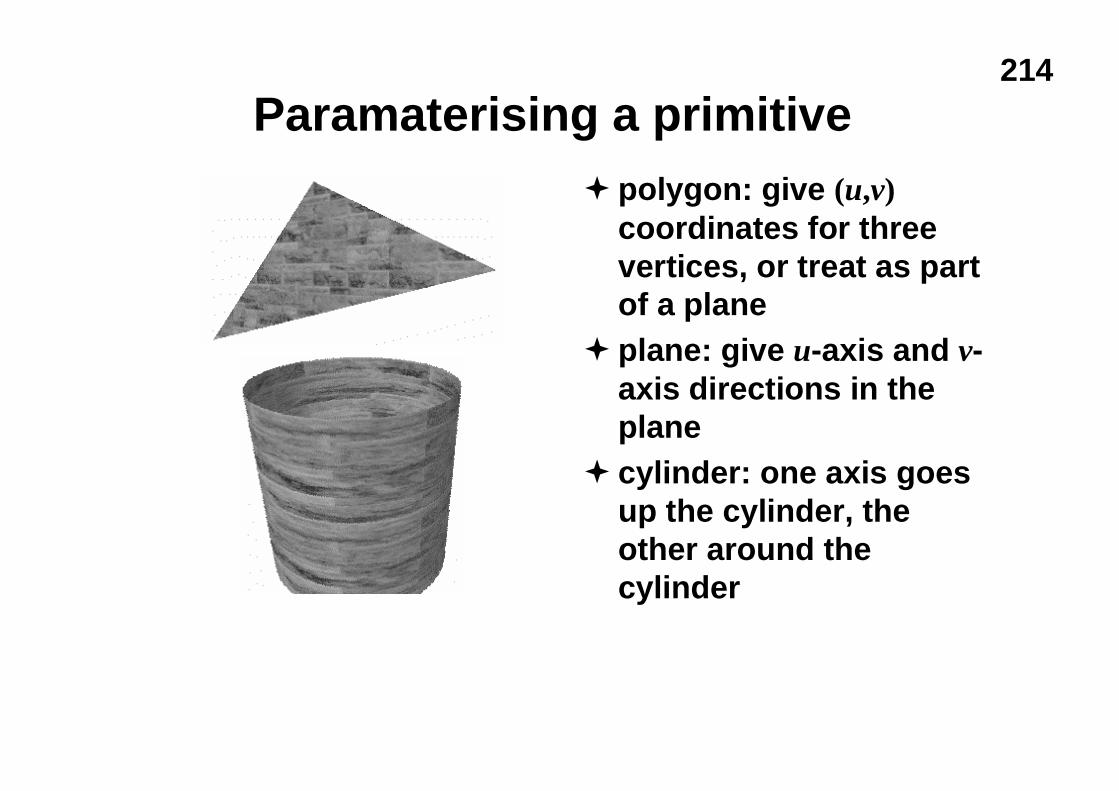
214

Paramaterising a primitive� polygon: give (u,v)

coordinates for threevertices, or treat as partof a plane

� plane: give u-axis and v-axis directions in theplane

� cylinder: one axis goesup the cylinder, theother around thecylinder

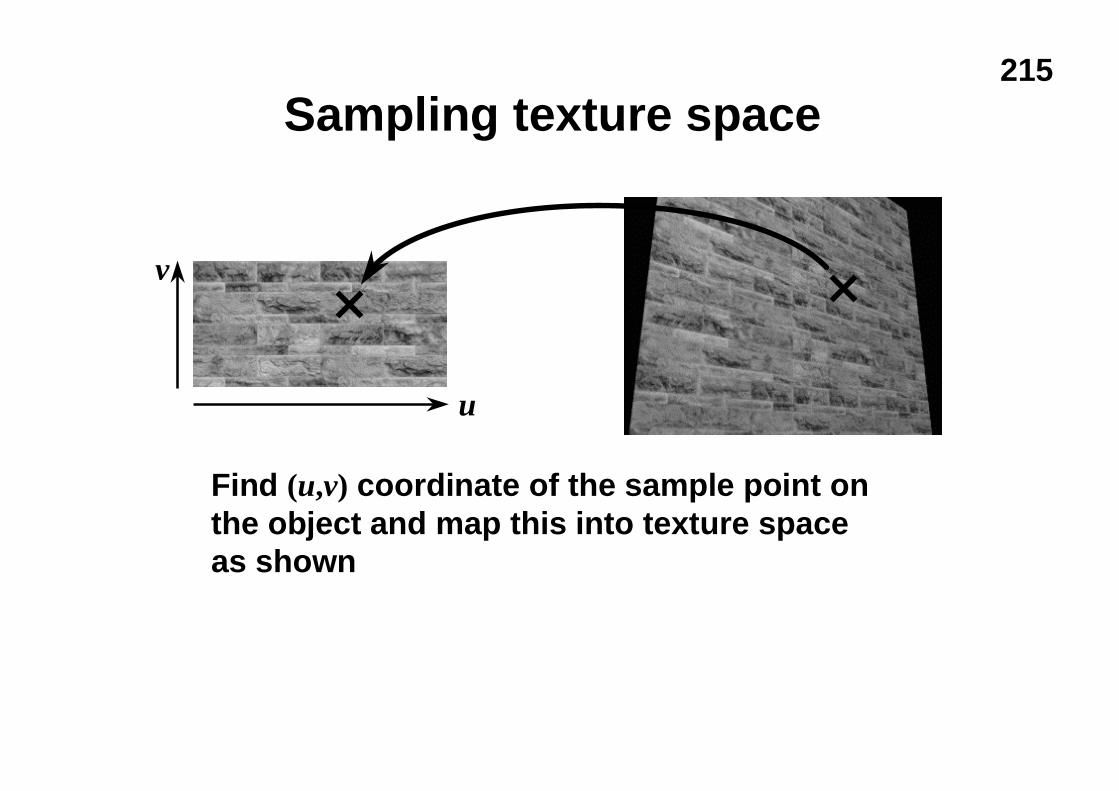
215

Sampling texture space

u

v

Find (u,v) coordinate of the sample point onthe object and map this into texture spaceas shown

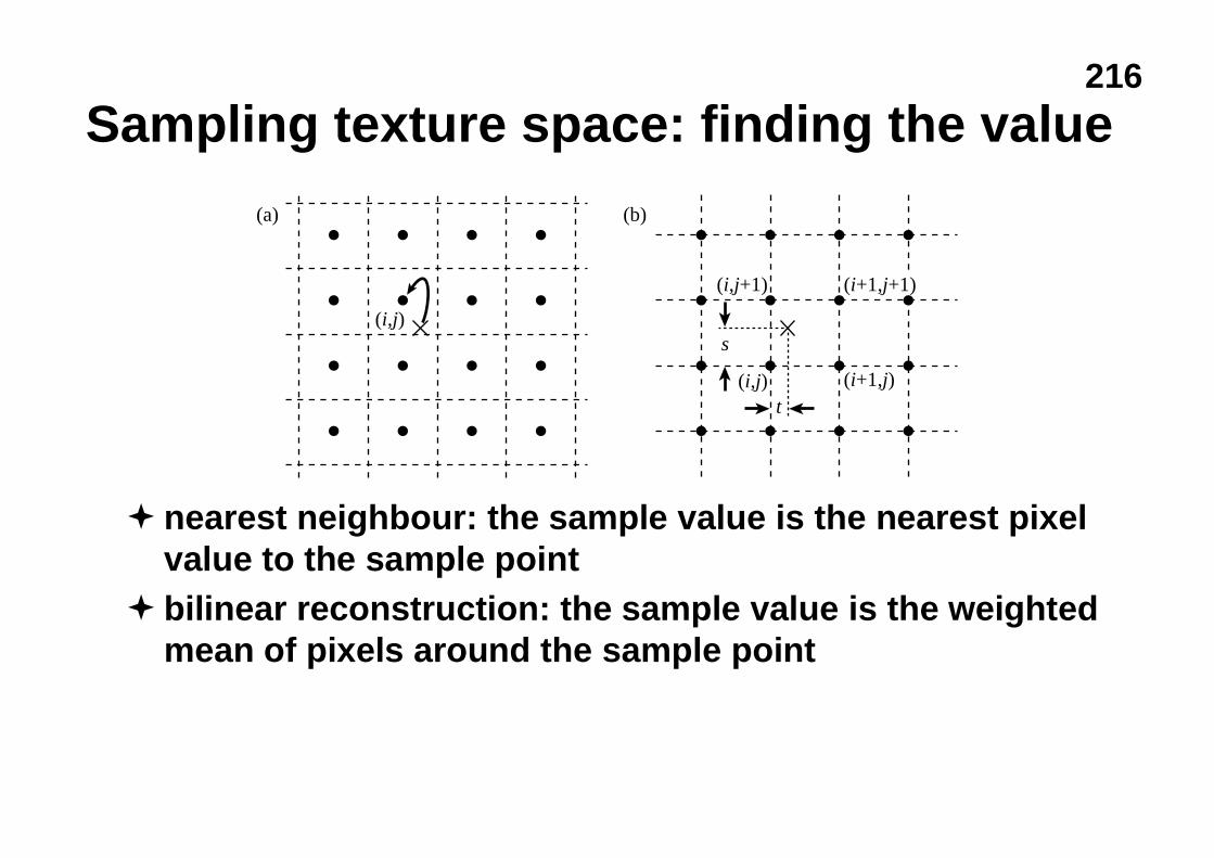
216

Sampling texture space: finding the value

� nearest neighbour: the sample value is the nearest pixelvalue to the sample point

� bilinear reconstruction: the sample value is the weightedmean of pixels around the sample point

(a) (b)

(i,j)

(i,j)

(i,j+1)

(i+1,j)

(i+1,j+1)

t

s

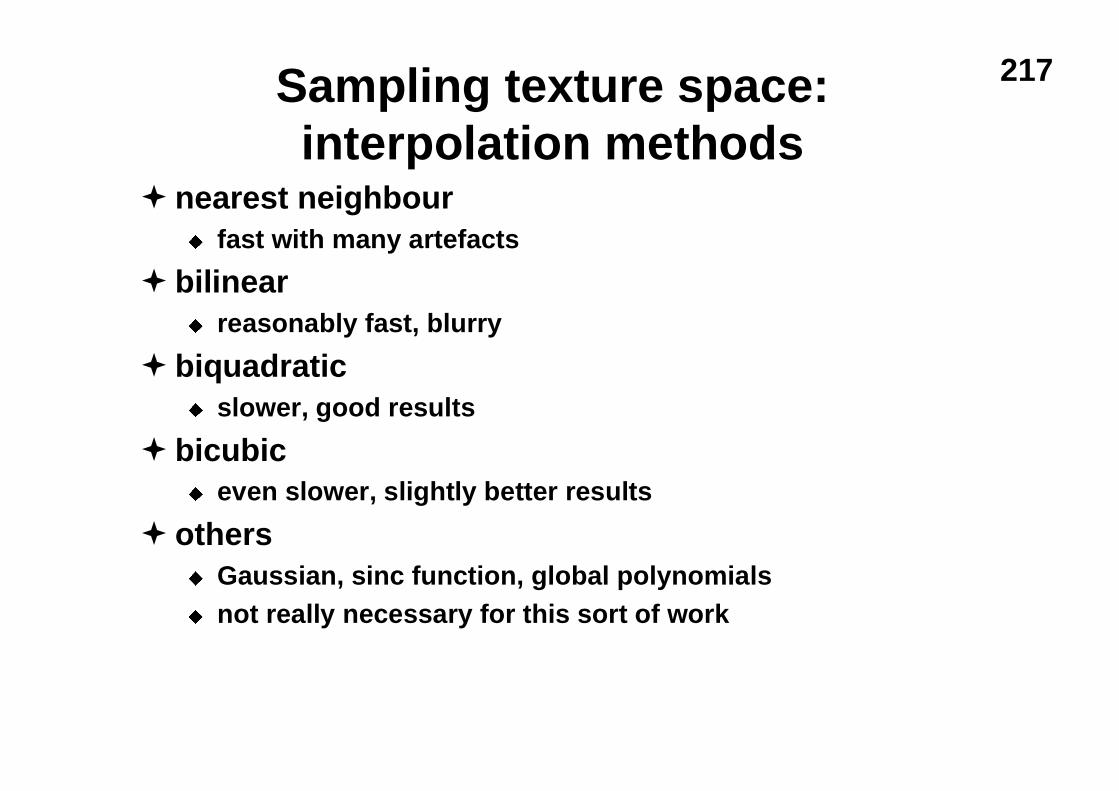
217Sampling texture space:interpolation methods

� nearest neighbouru fast with many artefacts

� bilinearu reasonably fast, blurry

� biquadraticu slower, good results

� bicubicu even slower, slightly better results

� othersu Gaussian, sinc function, global polynomialsu not really necessary for this sort of work

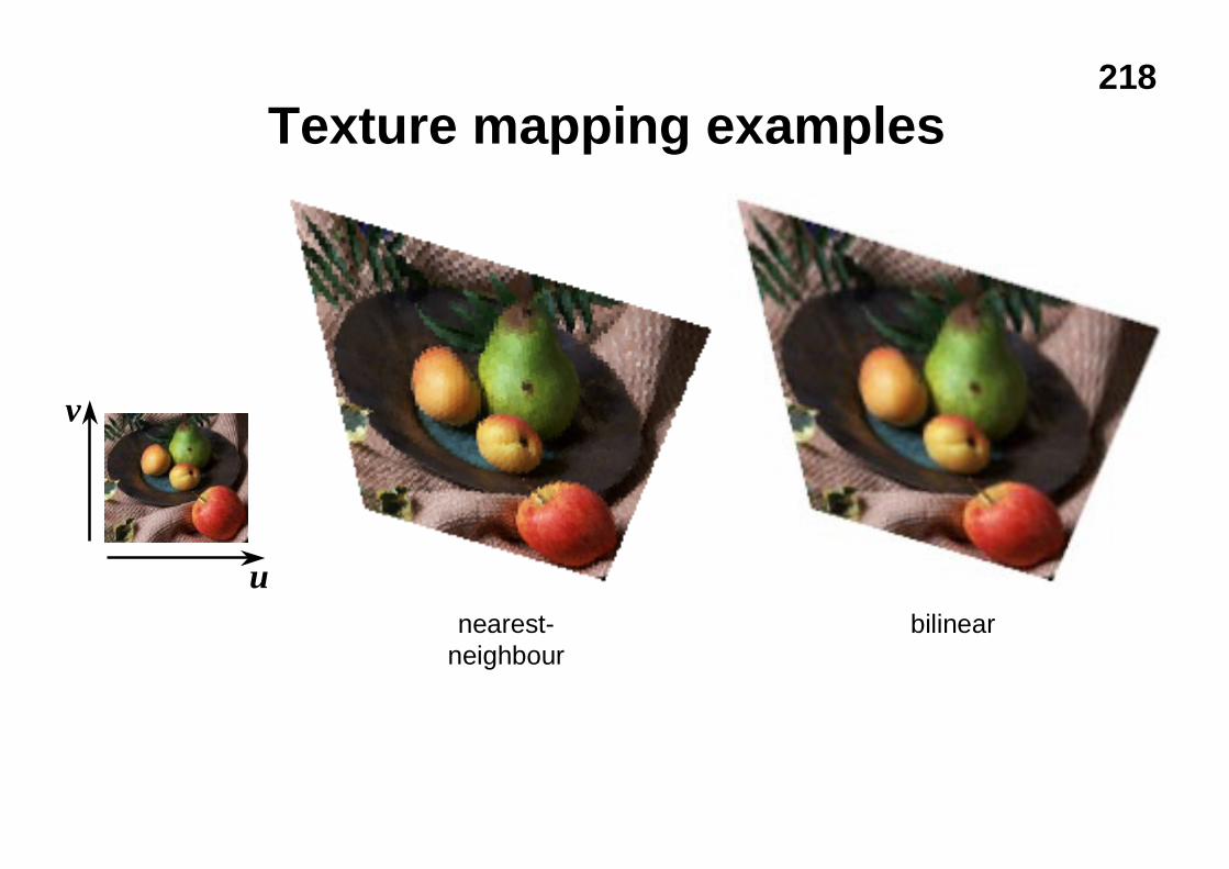
218

Texture mapping examples

nearest-neighbour

bilinear

u

v

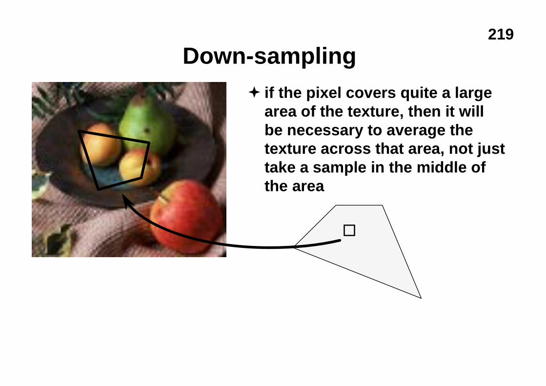
219

Down-sampling� if the pixel covers quite a large

area of the texture, then it willbe necessary to average thetexture across that area, not justtake a sample in the middle ofthe area

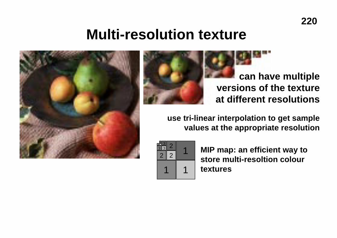
220

Multi-resolution texture

can have multipleversions of the textureat different resolutions

3 33

2 2

2

1 1

1 MIP map: an efficient way tostore multi-resoltion colourtextures

use tri-linear interpolation to get samplevalues at the appropriate resolution

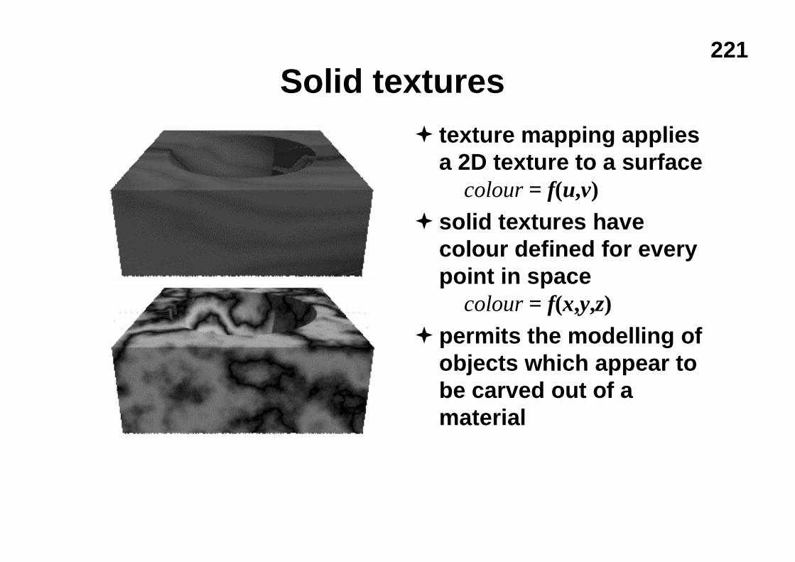
221

Solid textures� texture mapping applies

a 2D texture to a surface colour = f(u,v)

� solid textures havecolour defined for everypoint in space colour = f(x,y,z)

� permits the modelling ofobjects which appear tobe carved out of amaterial

222

What can a texture map modify?

�any (or all) of the colour componentsu ambient, diffuse, specular

�transparencyu “transparency mapping”

�reflectiveness

�but also the surface normalu “bump mapping”

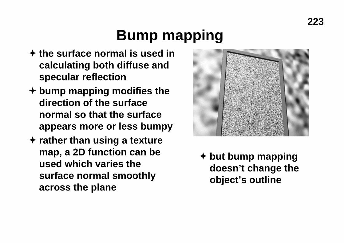
223

Bump mapping

� but bump mappingdoesn’t change theobject’s outline

� the surface normal is used incalculating both diffuse andspecular reflection

� bump mapping modifies thedirection of the surfacenormal so that the surfaceappears more or less bumpy

� rather than using a texturemap, a 2D function can beused which varies thesurface normal smoothlyacross the plane

223

Image Processingu filtering

n convolutionn nonlinear filtering

u point processingn intensity/colour correction

u compositingu halftoning & ditheringu compression

n various coding schemes

IP

Background

2D CG

3D CG

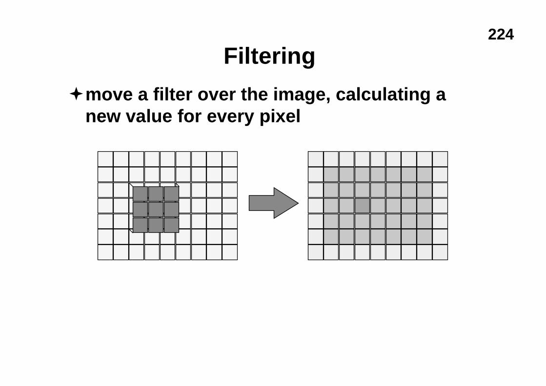
224

Filtering

�move a filter over the image, calculating anew value for every pixel

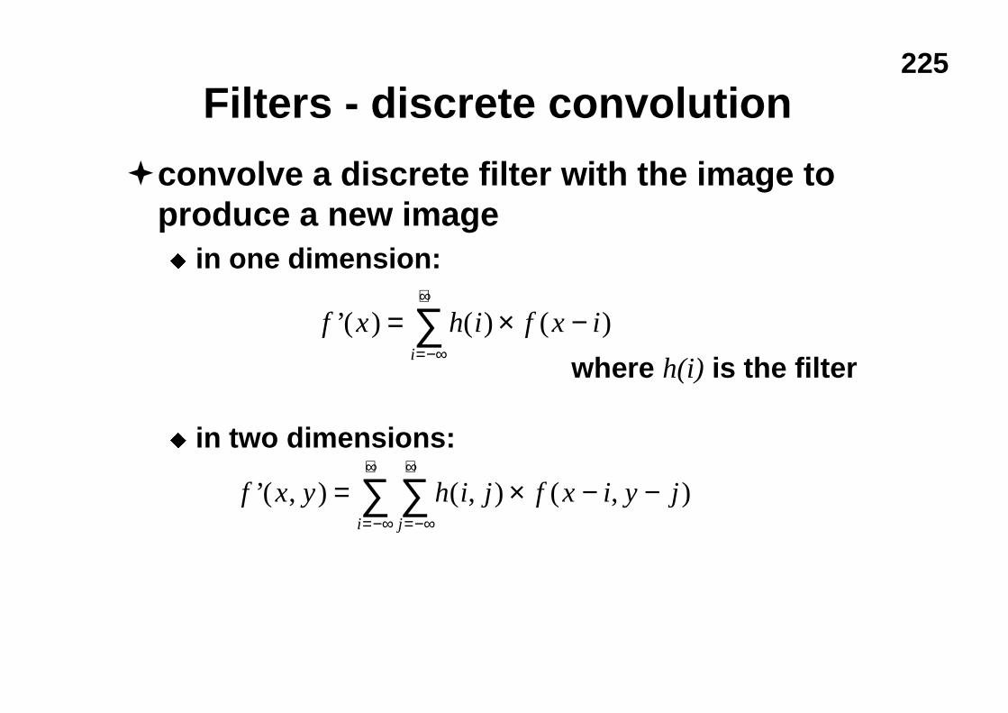
225

Filters - discrete convolution

�convolve a discrete filter with the image toproduce a new imageu in one dimension:

u in two dimensions:

f x h i f x ii

’( ) ( ) ( )= × −=−∞

+∞

∑where h(i) is the filter

f x y h i j f x i y jji

’( , ) ( , ) ( , )= × − −=−∞

+∞

=−∞

+∞

∑∑

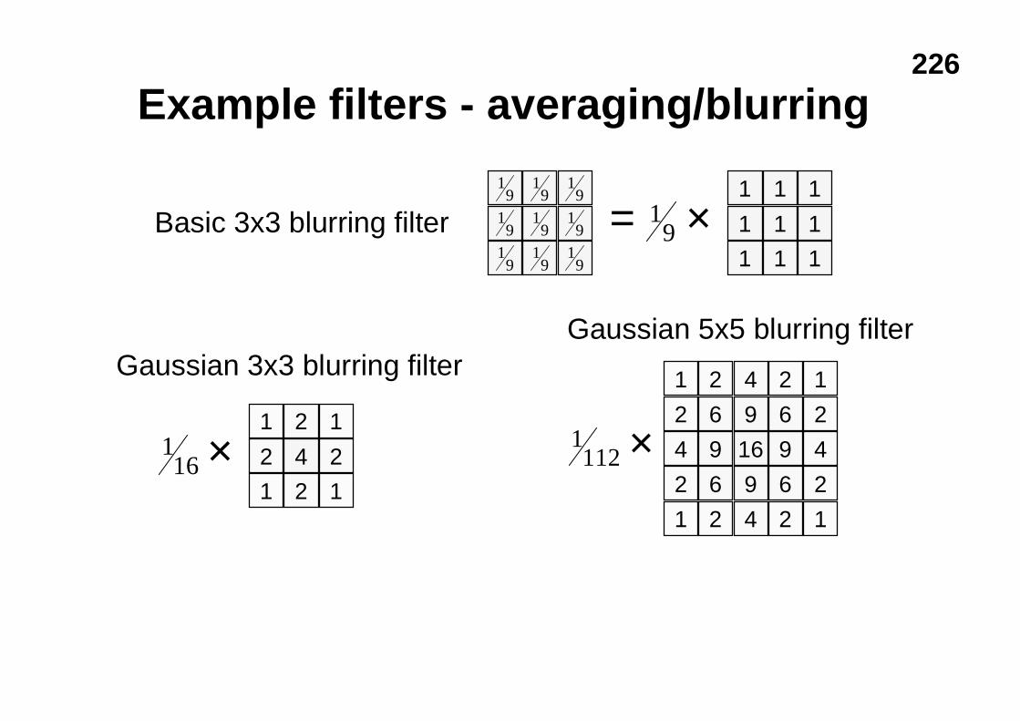
226

Example filters - averaging/blurring

19

19

19

19

19

19

19

19

19

1 1 1

1 1 1

1 1 1

= ×19

1 2 1

2 24

1 2 1

116 ×

1 2 4 2 1

2

4

2

1 2 4 2 1

2

4

2

6 6

6 69

9

9

9161112 ×

Basic 3x3 blurring filter

Gaussian 3x3 blurring filterGaussian 5x5 blurring filter

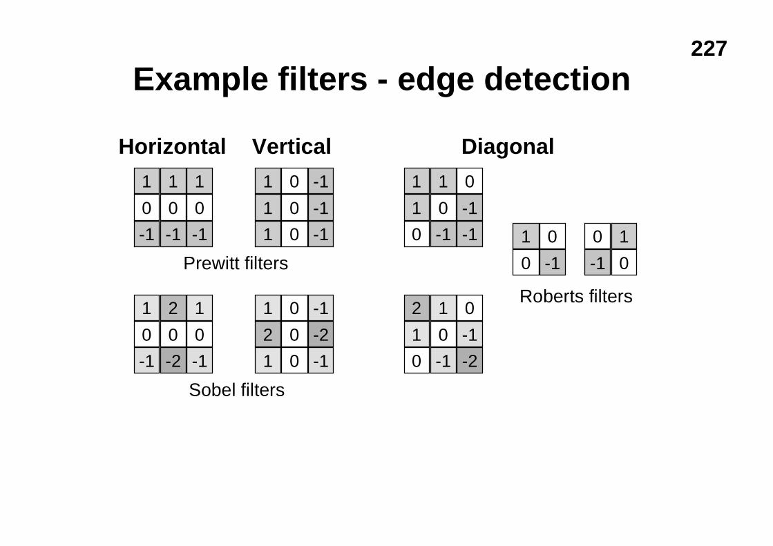
227

Example filters - edge detection

1 1 1

0 00

-1 -1 -1

1 1 0

1 -10

0 -1 -1

1 0 -1

1 -10

1 0 -1

1 2 1

0 00

-1 -2 -1

2 1 0

1 -10

0 -1 -2

1 0 -1

2 -20

1 0 -1

1 0

-10

0 1

0-1Prewitt filters

Sobel filters

Roberts filters

Horizontal Vertical Diagonal

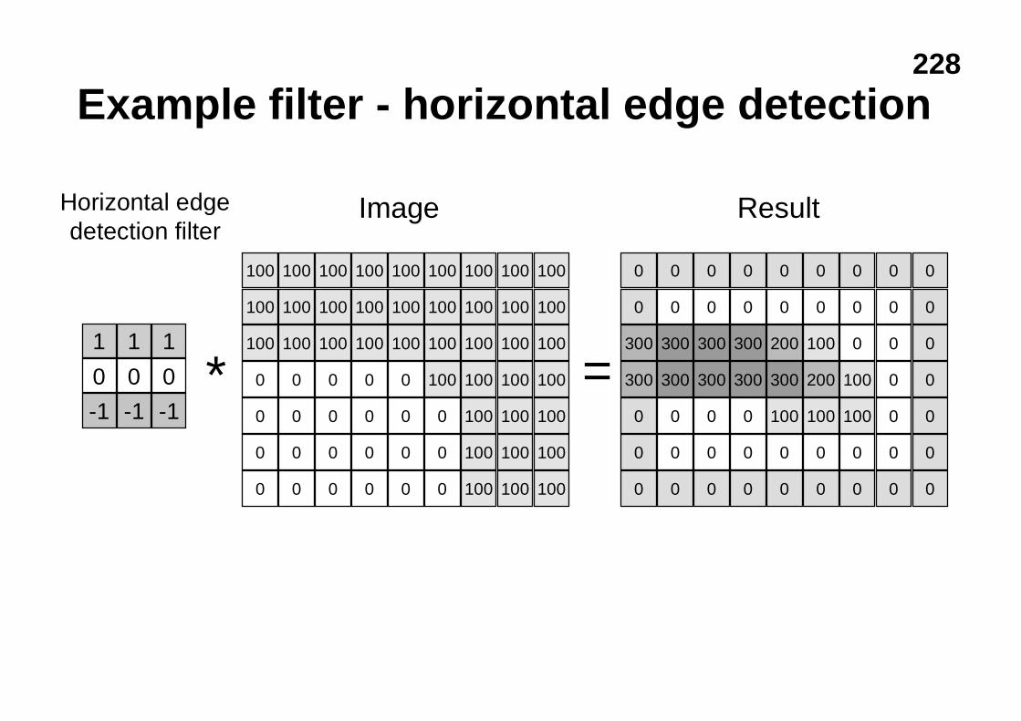
228

Example filter - horizontal edge detection

1 1 1

0 00

-1 -1 -1

300 200 100 0

300 300 200 100

0 100 100 100

0 0 0 0 0 0

0 0 0 0

0

300

300

0

0

0

0 0 0 0 0 00

0 0 0 0 0

300

300

0

0

0

0

0

0

0

0

0

0

0

0

0

0

0

0

0

300

300

0

0

100 100 100 100 100 100

100 100 100 100 100 100

0 0 0 100 100 100

0 0 0 0 100 100

0 0 0 0 100 100

0 0 0 0 100 100

100 100 100 100 100 100

100

100

0

0

0

0

100

100

100

100

100

100

100

100

100

100

0

0

0

0

100

∗ =

Horizontal edgedetection filter

Image Result

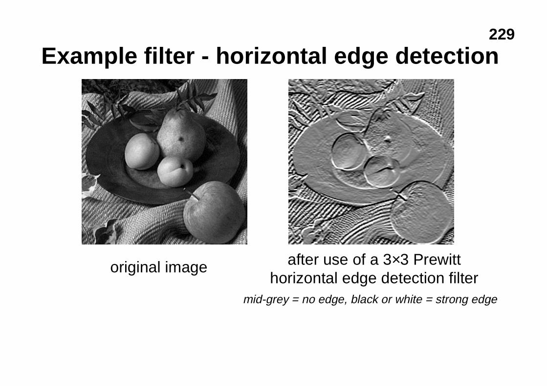
229

Example filter - horizontal edge detection

original image after use of a 3×3 Prewitthorizontal edge detection filter

mid-grey = no edge, black or white = strong edge

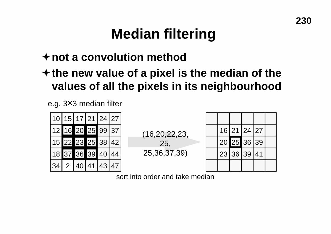
230

Median filtering

�not a convolution method�the new value of a pixel is the median of the

values of all the pixels in its neighbourhood

99

10 15

12

15

17 21 24

18

27

34 2

37

38 42

40 44

40 41 43 47

16 20 25

22 23 25

37 36 39

27

39

41

16 21 24

20 36

23 36 39

25(16,20,22,23,

25,25,36,37,39)

sort into order and take median

e.g. 3×3 median filter

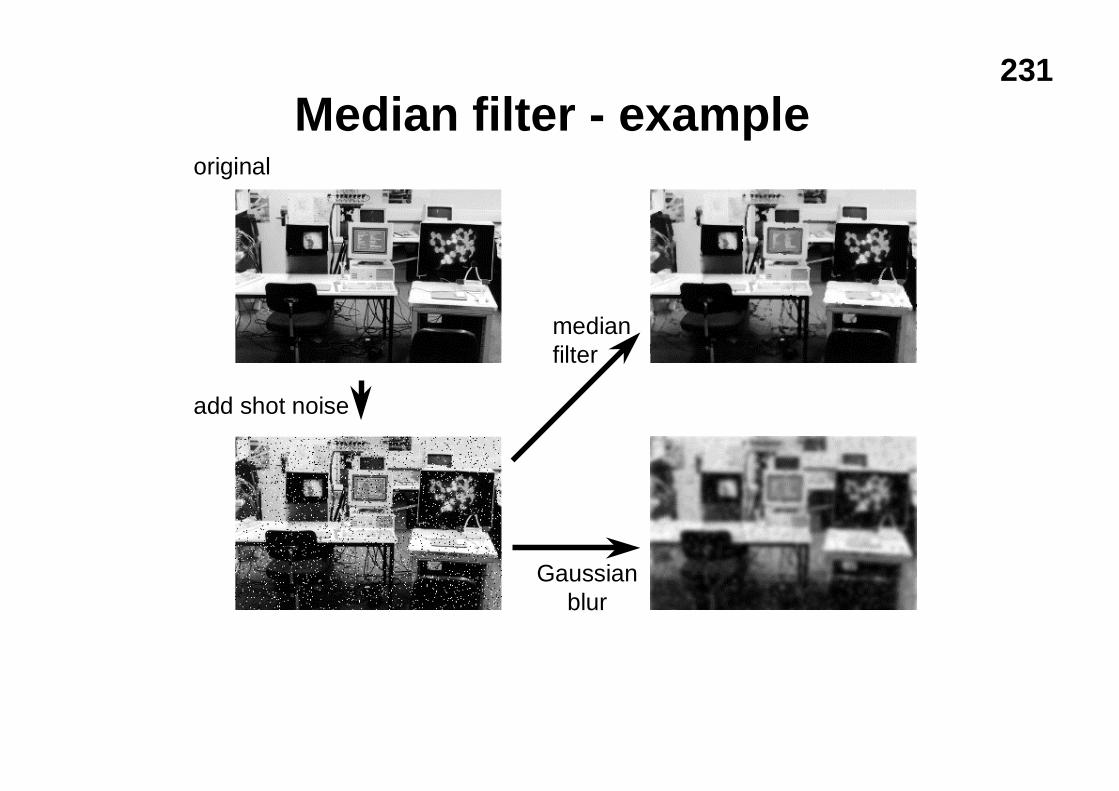
231

Median filter - exampleoriginal

add shot noise

medianfilter

Gaussianblur

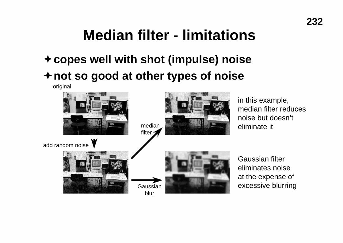
232

Median filter - limitations

�copes well with shot (impulse) noise�not so good at other types of noise

original

add random noise

medianfilter

Gaussianblur

in this example,median filter reducesnoise but doesn’teliminate it

Gaussian filtereliminates noiseat the expense ofexcessive blurring

233

Point processing

�each pixel’s value is modified�the modification function only takes that

pixel’s value into account

u where p(i,j) is the value of the pixel and p’(i,j) is themodified value

u the modification function, f (p), can perform anyoperation that maps one intensity value to another

p i j f p i j’( , ) { ( , )}=

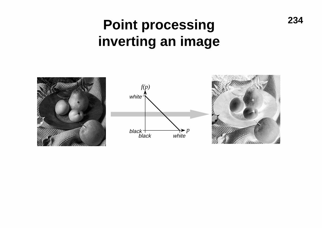
234Point processinginverting an image

black

white

p

f(p)

black white

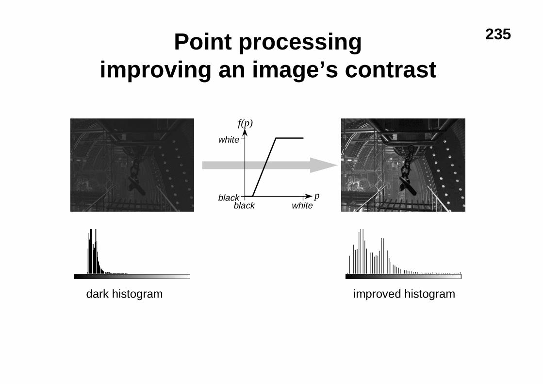
235Point processingimproving an image’s contrast

black

white

p

f(p)

black white

dark histogram improved histogram

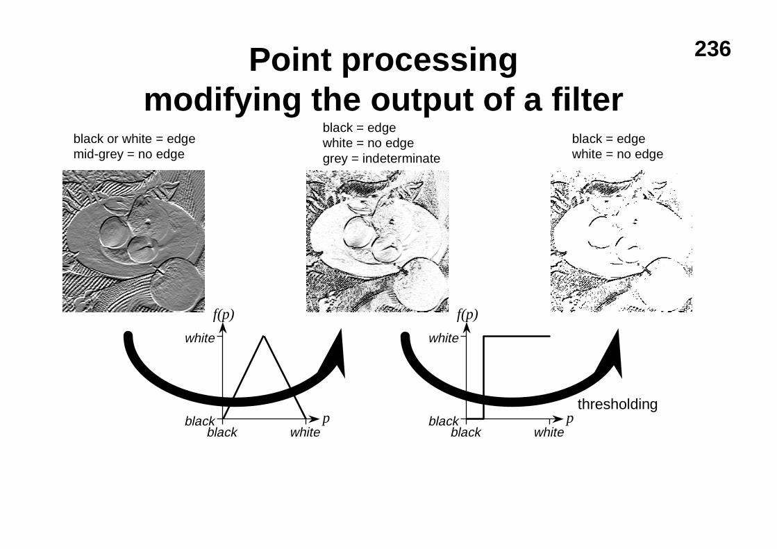
236Point processingmodifying the output of a filter

black

white

p

f(p)

black whiteblack

white

p

f(p)

black white

black or white = edgemid-grey = no edge

black = edgewhite = no edgegrey = indeterminate

black = edgewhite = no edge

thresholding

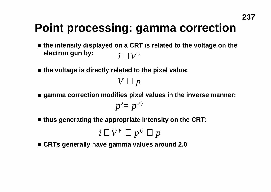
237

Point processing: gamma correctionn the intensity displayed on a CRT is related to the voltage on the

electron gun by:

n the voltage is directly related to the pixel value:

n gamma correction modifies pixel values in the inverse manner:

n thus generating the appropriate intensity on the CRT:

n CRTs generally have gamma values around 2.0

i V∝ γ

p p’ /= 1 γ

V p∝

i V p p∝ ∝ ∝γ γ’

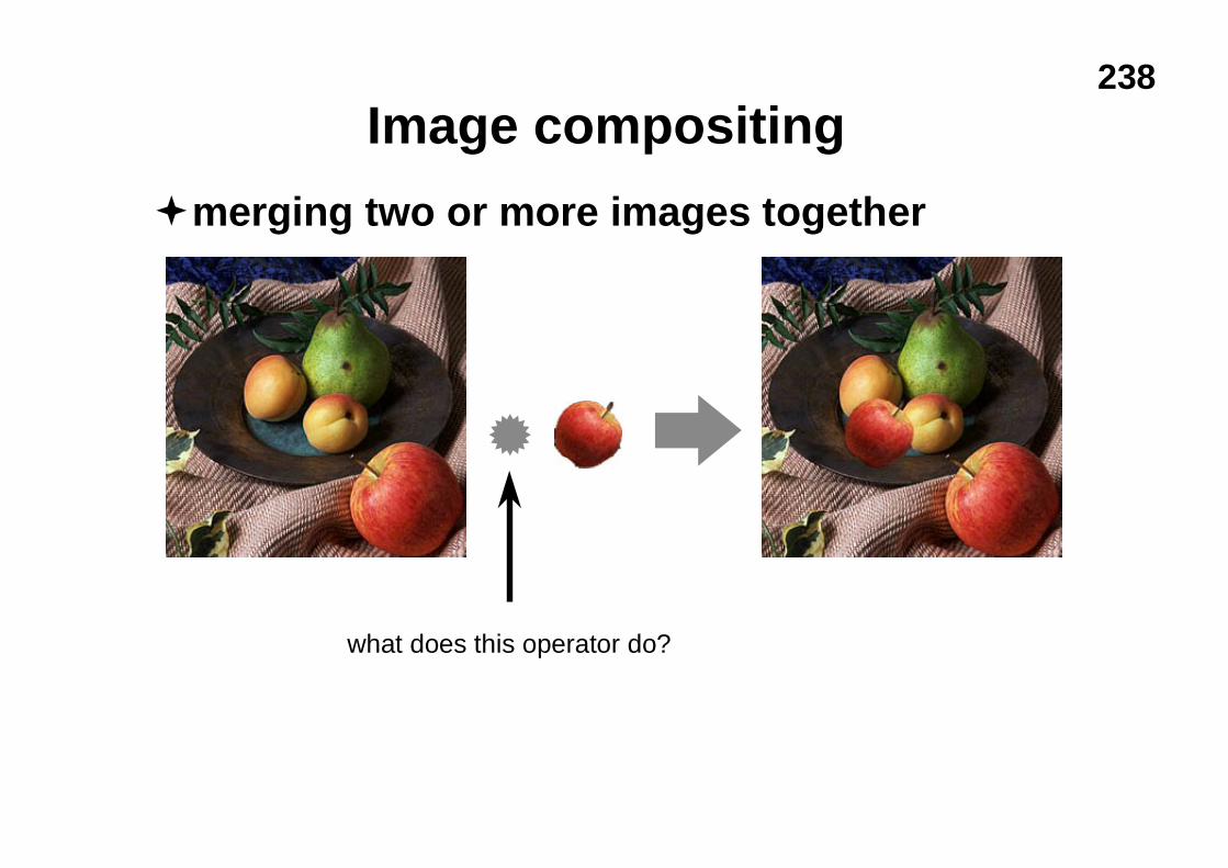
238

Image compositing

�merging two or more images together

what does this operator do?

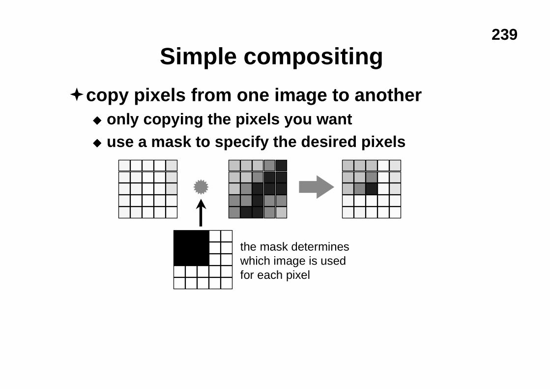
239

Simple compositing

�copy pixels from one image to anotheru only copying the pixels you wantu use a mask to specify the desired pixels

the mask determineswhich image is usedfor each pixel

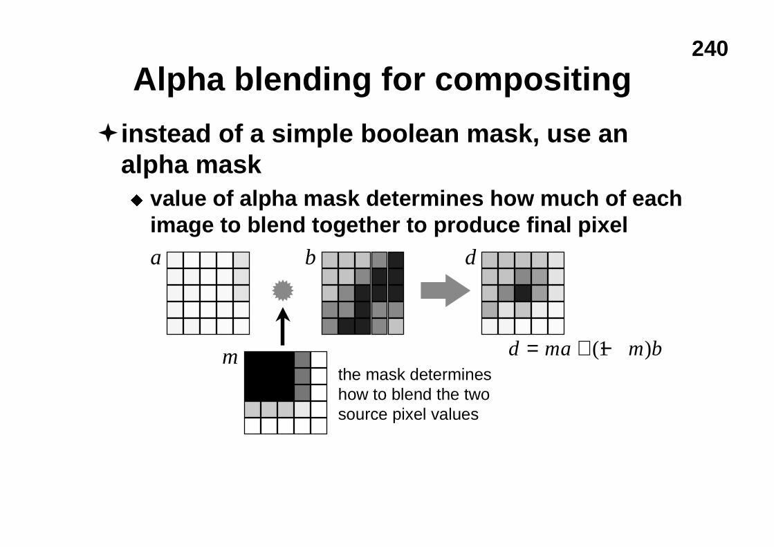
240

Alpha blending for compositing

�instead of a simple boolean mask, use analpha masku value of alpha mask determines how much of each

image to blend together to produce final pixel

the mask determineshow to blend the twosource pixel values

a b

m d ma m b= + −( )1

d

241

Arithmetic operations

�images can be manipulated arithmeticallyu simply apply the operation to each pixel location

in turn

�multiplicationu used in masking

�subtraction (difference)u used to compare imagesu e.g. comparing two x-ray images before and after

injection of a dye into the bloodstream

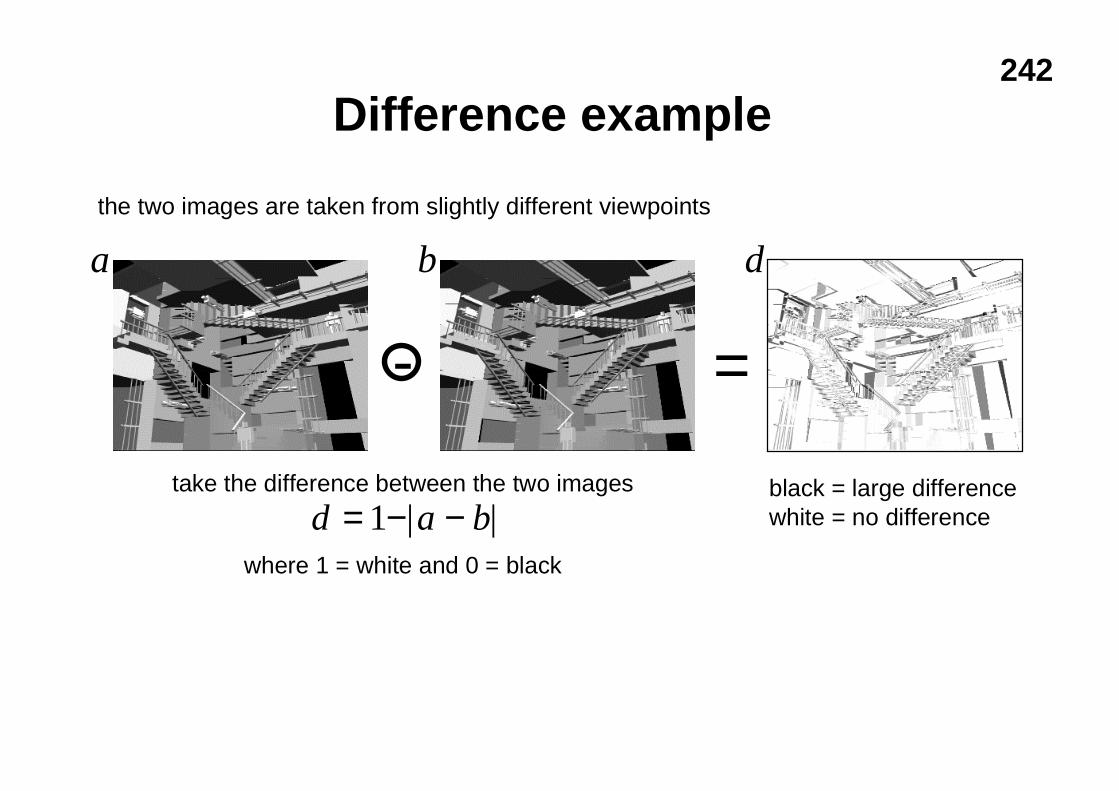
242

Difference example

- =

take the difference between the two images black = large differencewhite = no differenced a b= − −1 | |

a b d

where 1 = white and 0 = black

the two images are taken from slightly different viewpoints

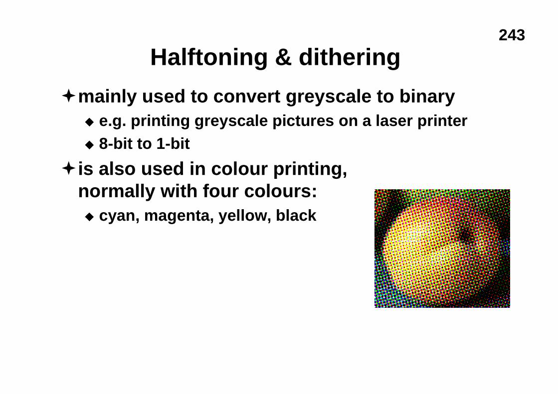
243

Halftoning & dithering

�mainly used to convert greyscale to binaryu e.g. printing greyscale pictures on a laser printeru 8-bit to 1-bit

�is also used in colour printing,normally with four colours:u cyan, magenta, yellow, black

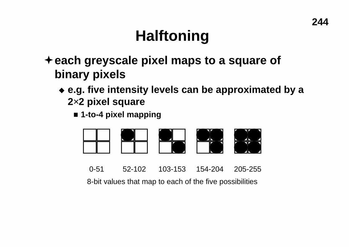
244

Halftoning

�each greyscale pixel maps to a square ofbinary pixelsu e.g. five intensity levels can be approximated by a

2×2 pixel squaren 1-to-4 pixel mapping

8-bit values that map to each of the five possibilities

0-51 52-102 103-153 154-204 205-255

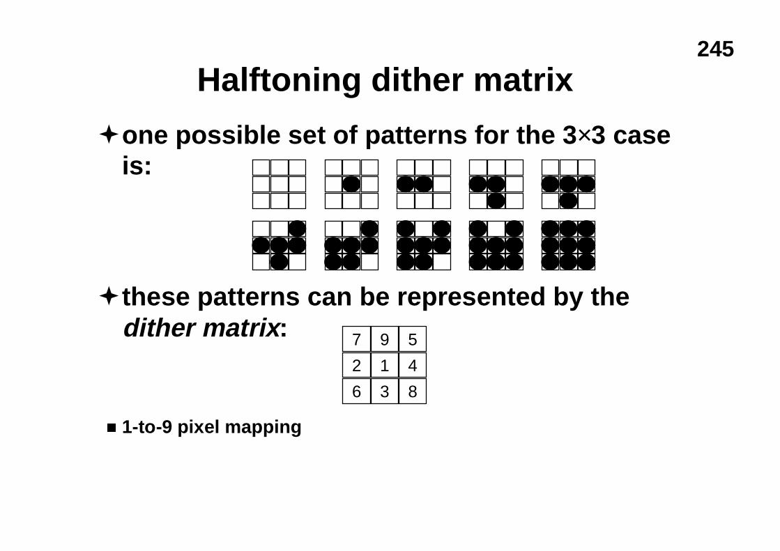
245

Halftoning dither matrix

�one possible set of patterns for the 3×3 caseis:

�these patterns can be represented by thedither matrix: 7 9 5

2 1 4

6 3 8

n 1-to-9 pixel mapping

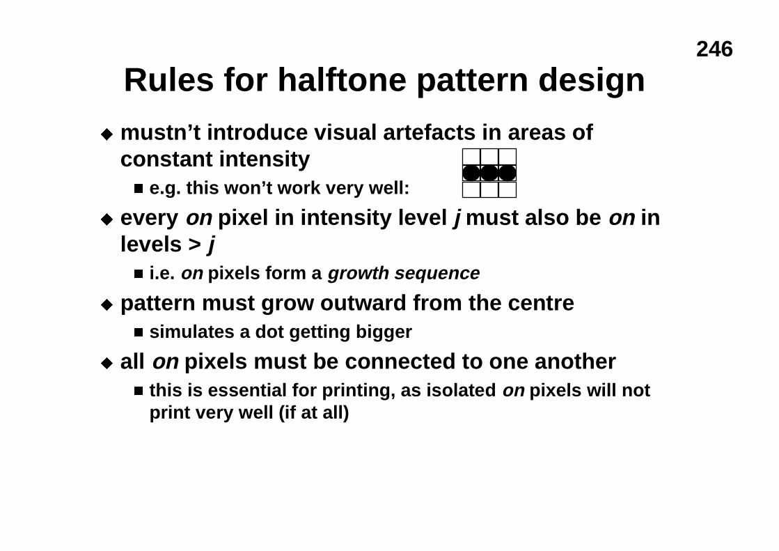
246

Rules for halftone pattern designu mustn’t introduce visual artefacts in areas of

constant intensityn e.g. this won’t work very well:

u every on pixel in intensity level j must also be on inlevels > jn i.e. on pixels form a growth sequence

u pattern must grow outward from the centren simulates a dot getting bigger

u all on pixels must be connected to one anothern this is essential for printing, as isolated on pixels will not

print very well (if at all)

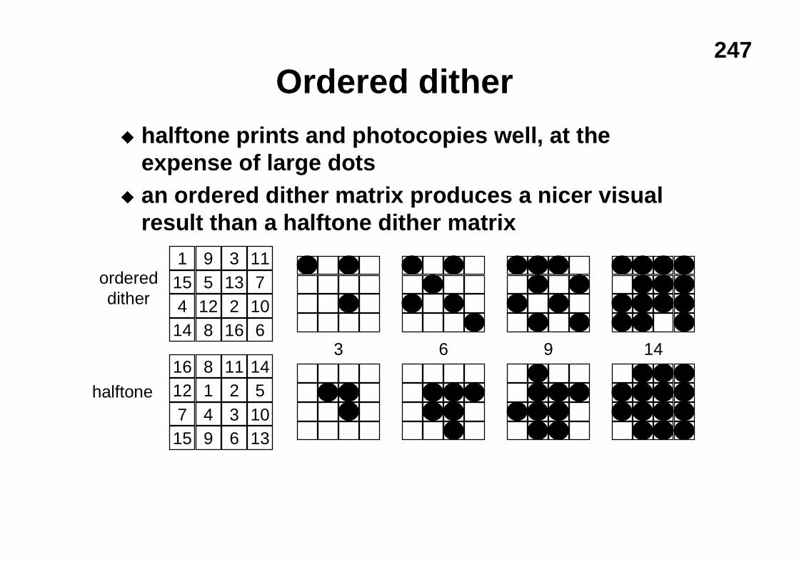
247

Ordered ditheru halftone prints and photocopies well, at the

expense of large dotsu an ordered dither matrix produces a nicer visual

result than a halftone dither matrix

1 9 3 1115 5 13 74 12 2 10

14 8 16 6

16 8 11 1412 1 2 57 4 3 10

15 9 6 13

ordereddither

halftone

3 6 9 14

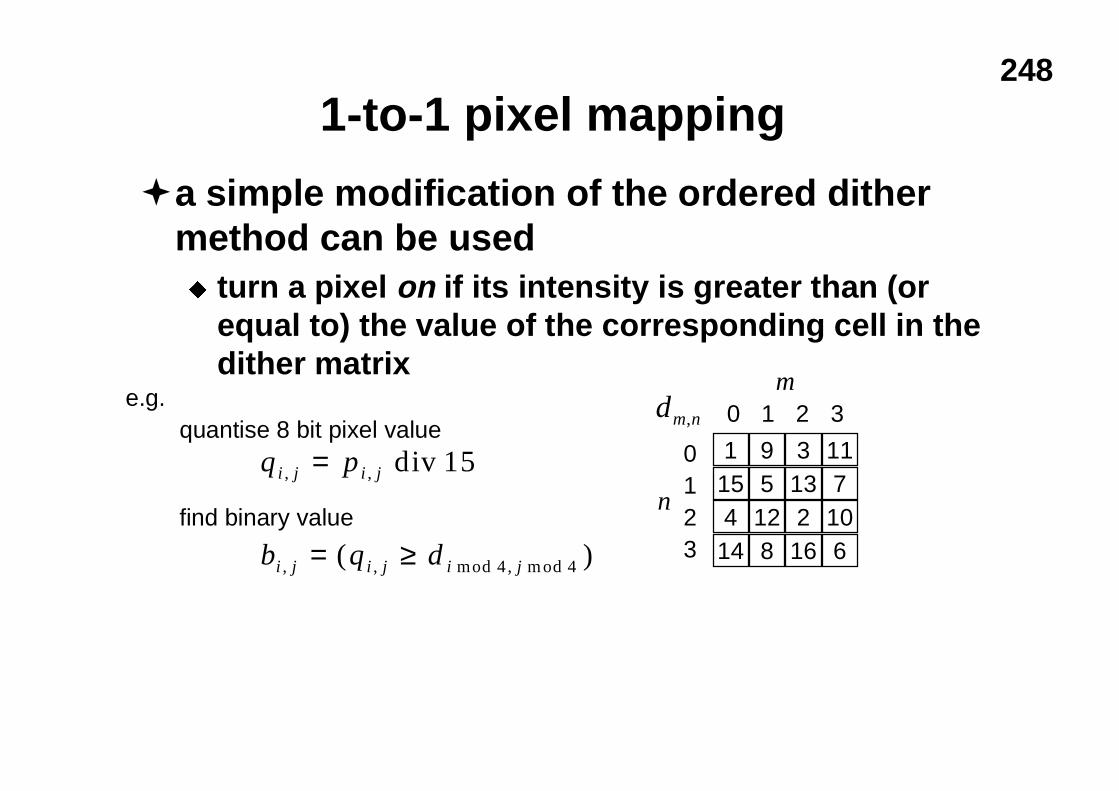
248

1-to-1 pixel mapping

�a simple modification of the ordered dithermethod can be usedu turn a pixel on if its intensity is greater than (or

equal to) the value of the corresponding cell in thedither matrix

1 9 3 1115 5 13 74 12 2 10

14 8 16 6

0 1 2 3

0123

m

n

dm n,

q p

b q d

i j i j

i j i j i j

, ,

, , ,( )

=

= ≥

div

mod mod

15

4 4

quantise 8 bit pixel value

find binary value

e.g.

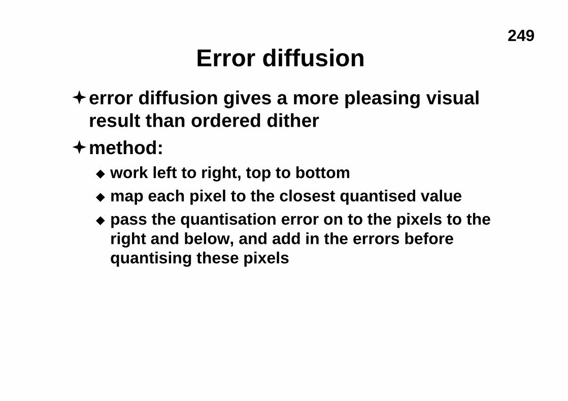
249

Error diffusion

�error diffusion gives a more pleasing visualresult than ordered dither

�method:u work left to right, top to bottomu map each pixel to the closest quantised valueu pass the quantisation error on to the pixels to the

right and below, and add in the errors beforequantising these pixels

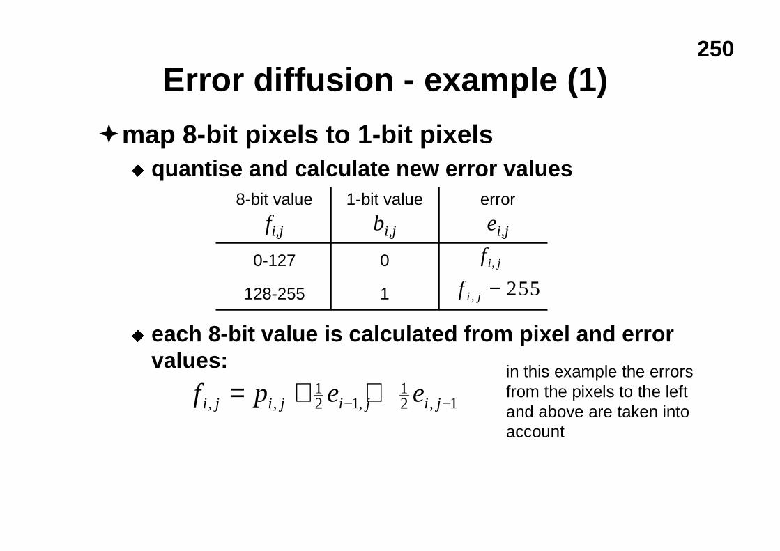
250

Error diffusion - example (1)

�map 8-bit pixels to 1-bit pixelsu quantise and calculate new error values

u each 8-bit value is calculated from pixel and errorvalues:

8-bit value

fi,j

1-bit value

bi,j

error

ei,j

0-127

128-255

0

1

f i j,

f i j, − 255

f p e ei j i j i j i j, , , ,= + +− −12 1

12 1

in this example the errorsfrom the pixels to the leftand above are taken intoaccount

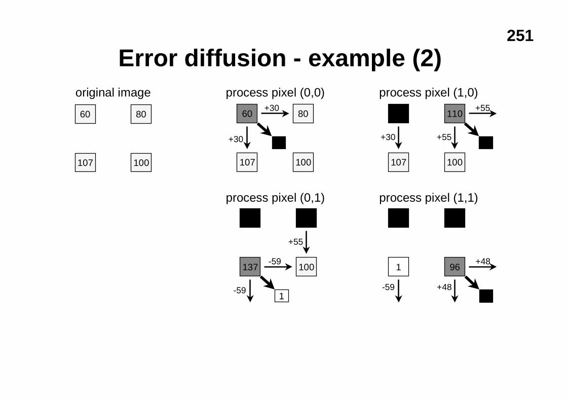
251

Error diffusion - example (2)

107 100

60 80

+30

107 100

60 80

0

+30

1

137 100

0 0

+55

-59

-591 96

0 0

0-59 +48

+48

original image process pixel (0,0) process pixel (1,0)

process pixel (0,1) process pixel (1,1)

107 100

0 110

+30 +55

+55

0

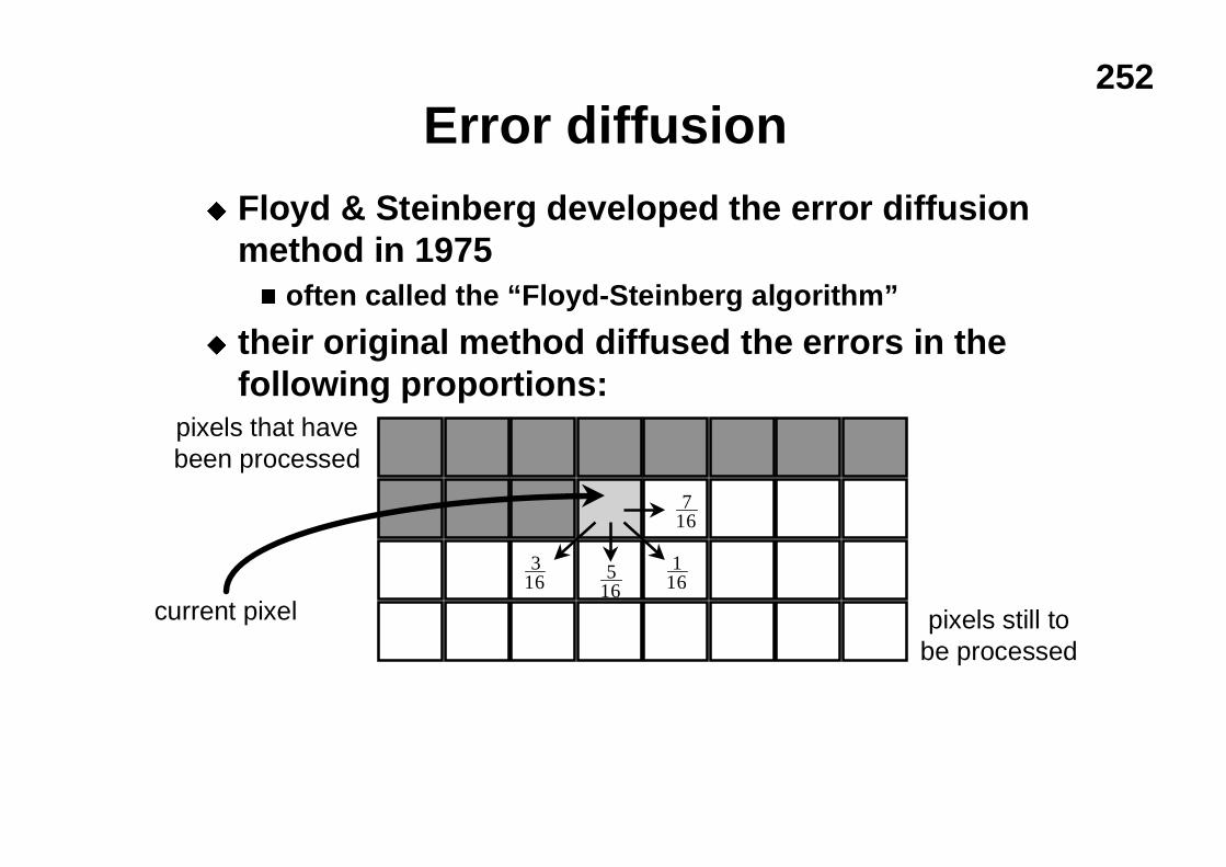
252

Error diffusionu Floyd & Steinberg developed the error diffusion

method in 1975n often called the “Floyd-Steinberg algorithm”

u their original method diffused the errors in thefollowing proportions:

716

1165

16

316

pixels still tobe processed

pixels that havebeen processed

current pixel

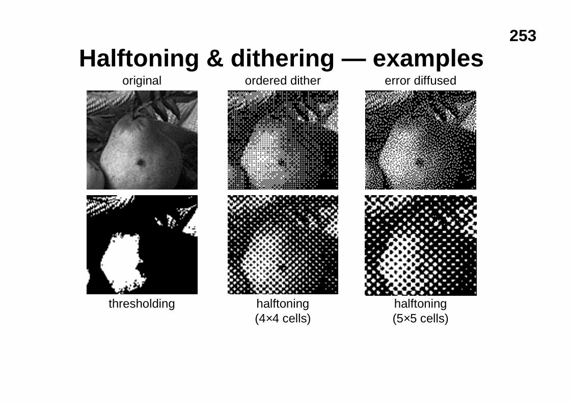
253

Halftoning & dithering — examplesordered dither

halftoning(4×4 cells)

error diffused

halftoning(5×5 cells)

original

thresholding

254

Halftoning & dithering — examplesoriginal

halftoned with a veryfine screen

ordered dither

the regular ditherpattern is clearlyvisible

error diffused

more random thanordered dither andtherefore looks moreattractive to thehuman eye

thresholding

<128 ⇒ black

≥128 ⇒ white

halftoning

the larger the cell size, the more intensity levelsavailable

the smaller the cell, the less noticable thehalftone dots

255

Encoding & compression

�introduction�various coding schemes

u difference, predictive, run-length, quadtree

�transform codingu Fourier, cosine, wavelets, JPEG

256

What you should note about image data

�there’s lots of it!u an A4 page scanned at 300 ppi produces:

n 24MB of data in 24 bit per pixel colourn 1MB of data at 1 bit per pixel

l the Encyclopaedia Britannica would require 25GB at 300ppi, 1 bit per pixel

�adjacent pixels tend to be very similar

�compression is therefore both feasible andnecessary

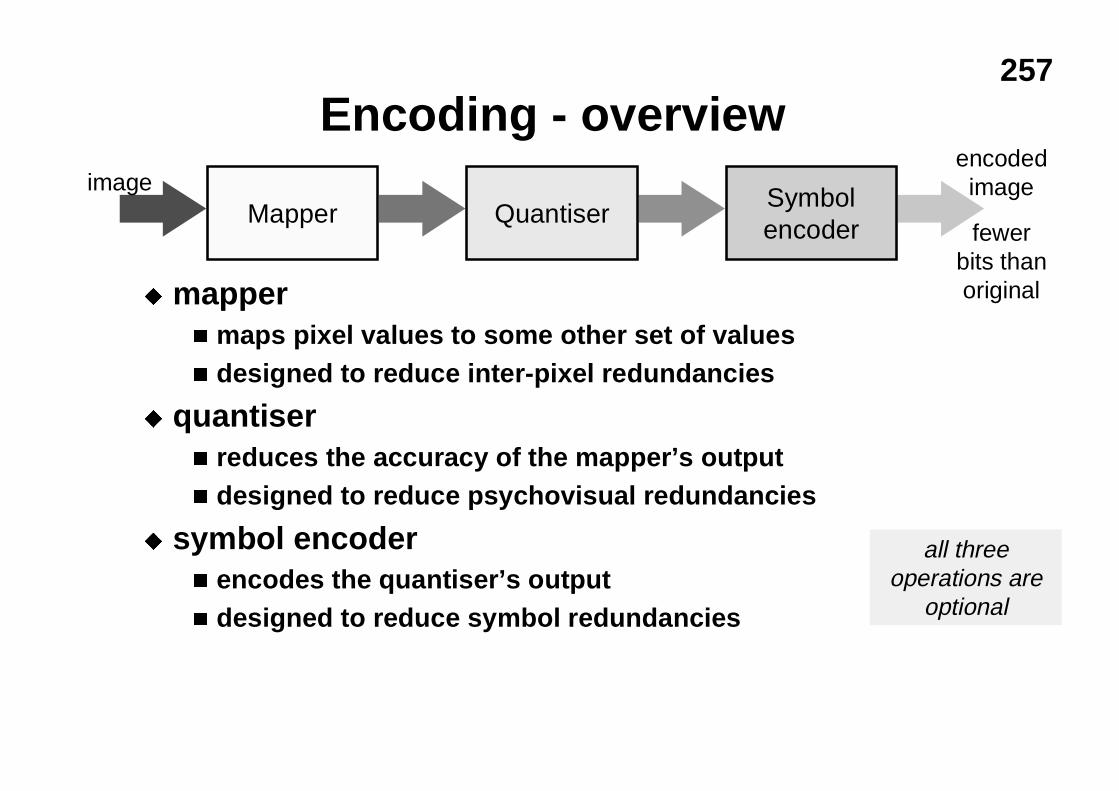
257

Encoding - overview

u mappern maps pixel values to some other set of valuesn designed to reduce inter-pixel redundancies

u quantisern reduces the accuracy of the mapper’s outputn designed to reduce psychovisual redundancies

u symbol encodern encodes the quantiser’s outputn designed to reduce symbol redundancies

Mapper QuantiserSymbolencoder

imageencodedimage

all threeoperations are

optional

fewerbits thanoriginal

258

Lossless vs lossy compression

�losslessu allows you to exactly reconstruct the pixel values

from the encoded datan implies no quantisation stage and no losses in either of

the other stages

�lossyu loses some data, you cannot exactly reconstruct

the original pixel values

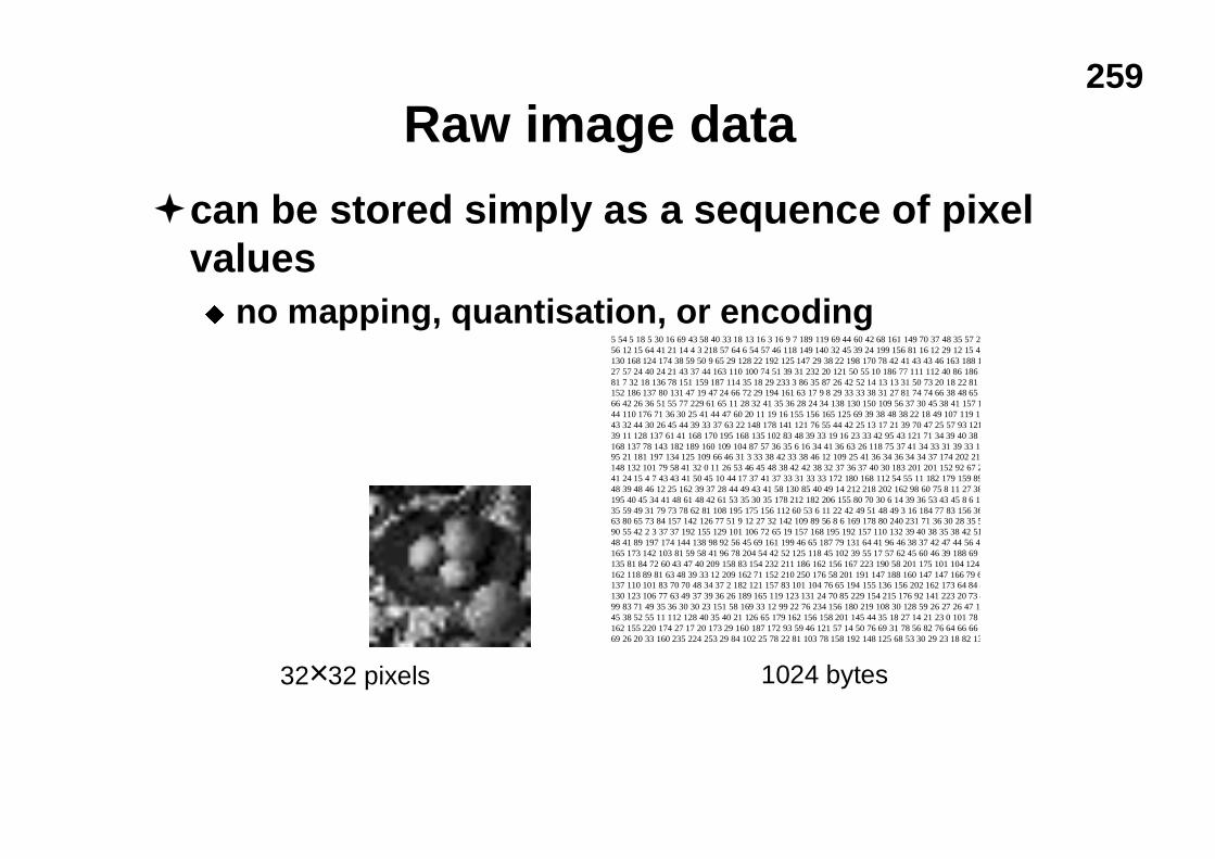
259

Raw image data

�can be stored simply as a sequence of pixelvaluesu no mapping, quantisation, or encoding

32×32 pixels 1024 bytes

5 54 5 18 5 30 16 69 43 58 40 33 18 13 16 3 16 9 7 189 119 69 44 60 42 68 161 149 70 37 48 35 57 2056 12 15 64 41 21 14 4 3 218 57 64 6 54 57 46 118 149 140 32 45 39 24 199 156 81 16 12 29 12 15 42130 168 124 174 38 59 50 9 65 29 128 22 192 125 147 29 38 22 198 170 78 42 41 43 43 46 163 188 127 57 24 40 24 21 43 37 44 163 110 100 74 51 39 31 232 20 121 50 55 10 186 77 111 112 40 86 186 81 7 32 18 136 78 151 159 187 114 35 18 29 233 3 86 35 87 26 42 52 14 13 13 31 50 73 20 18 22 81 152 186 137 80 131 47 19 47 24 66 72 29 194 161 63 17 9 8 29 33 33 38 31 27 81 74 74 66 38 48 65 66 42 26 36 51 55 77 229 61 65 11 28 32 41 35 36 28 24 34 138 130 150 109 56 37 30 45 38 41 157 144 110 176 71 36 30 25 41 44 47 60 20 11 19 16 155 156 165 125 69 39 38 48 38 22 18 49 107 119 143 32 44 30 26 45 44 39 33 37 63 22 148 178 141 121 76 55 44 42 25 13 17 21 39 70 47 25 57 93 12139 11 128 137 61 41 168 170 195 168 135 102 83 48 39 33 19 16 23 33 42 95 43 121 71 34 39 40 38 4168 137 78 143 182 189 160 109 104 87 57 36 35 6 16 34 41 36 63 26 118 75 37 41 34 33 31 39 33 1595 21 181 197 134 125 109 66 46 31 3 33 38 42 33 38 46 12 109 25 41 36 34 36 34 34 37 174 202 210148 132 101 79 58 41 32 0 11 26 53 46 45 48 38 42 42 38 32 37 36 37 40 30 183 201 201 152 92 67 241 24 15 4 7 43 43 41 50 45 10 44 17 37 41 37 33 31 33 33 172 180 168 112 54 55 11 182 179 159 8948 39 48 46 12 25 162 39 37 28 44 49 43 41 58 130 85 40 49 14 212 218 202 162 98 60 75 8 11 27 38195 40 45 34 41 48 61 48 42 61 53 35 30 35 178 212 182 206 155 80 70 30 6 14 39 36 53 43 45 8 6 1835 59 49 31 79 73 78 62 81 108 195 175 156 112 60 53 6 11 22 42 49 51 48 49 3 16 184 77 83 156 3663 80 65 73 84 157 142 126 77 51 9 12 27 32 142 109 89 56 8 6 169 178 80 240 231 71 36 30 28 35 590 55 42 2 3 37 37 192 155 129 101 106 72 65 19 157 168 195 192 157 110 132 39 40 38 35 38 42 5148 41 89 197 174 144 138 98 92 56 45 69 161 199 46 65 187 79 131 64 41 96 46 38 37 42 47 44 56 47165 173 142 103 81 59 58 41 96 78 204 54 42 52 125 118 45 102 39 55 17 57 62 45 60 46 39 188 69 6135 81 84 72 60 43 47 40 209 158 83 154 232 211 186 162 156 167 223 190 58 201 175 101 104 124 162 118 89 81 63 48 39 33 12 209 162 71 152 210 250 176 58 201 191 147 188 160 147 147 166 79 6137 110 101 83 70 70 48 34 37 2 182 121 157 83 101 104 76 65 194 155 136 156 202 162 173 64 84 8130 123 106 77 63 49 37 39 36 26 189 165 119 123 131 24 70 85 229 154 215 176 92 141 223 20 73 499 83 71 49 35 36 30 30 23 151 58 169 33 12 99 22 76 234 156 180 219 108 30 128 59 26 27 26 47 1245 38 52 55 11 112 128 40 35 40 21 126 65 179 162 156 158 201 145 44 35 18 27 14 21 23 0 101 78 7162 155 220 174 27 17 20 173 29 160 187 172 93 59 46 121 57 14 50 76 69 31 78 56 82 76 64 66 66 569 26 20 33 160 235 224 253 29 84 102 25 78 22 81 103 78 158 192 148 125 68 53 30 29 23 18 82 13

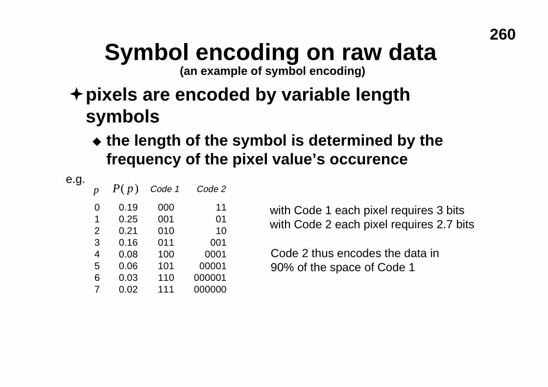
260Symbol encoding on raw data

�pixels are encoded by variable lengthsymbolsu the length of the symbol is determined by the

frequency of the pixel value’s occurence

01234567

0.190.250.210.160.080.060.030.02

000001010011100101110111

110110

0010001

00001000001000000

p P p( ) Code 1 Code 2

with Code 1 each pixel requires 3 bitswith Code 2 each pixel requires 2.7 bits

Code 2 thus encodes the data in90% of the space of Code 1

e.g.

(an example of symbol encoding)

261Quantisation as a compression method

�quantisation, on its own, is not normally usedfor compression because of the visualdegradation of the resulting image

�however, an 8-bit to 4-bit quantisation usingerror diffusion would compress an image to50% of the space

(an example of quantisation)

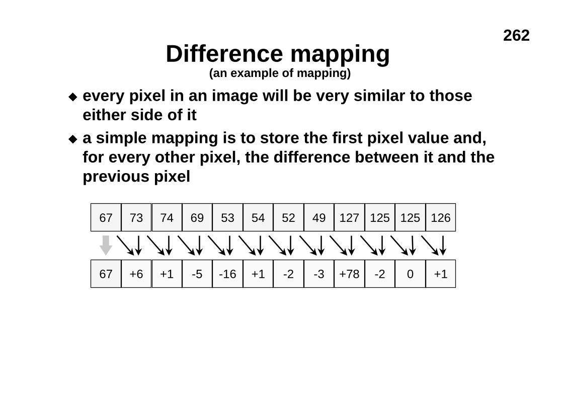
262Difference mapping

u every pixel in an image will be very similar to thoseeither side of it

u a simple mapping is to store the first pixel value and,for every other pixel, the difference between it and theprevious pixel

67 73 74 69 53 54 52 49 127 125 125 126

67 +6 +1 -5 -16 +1 -2 -3 +78 -2 0 +1

(an example of mapping)

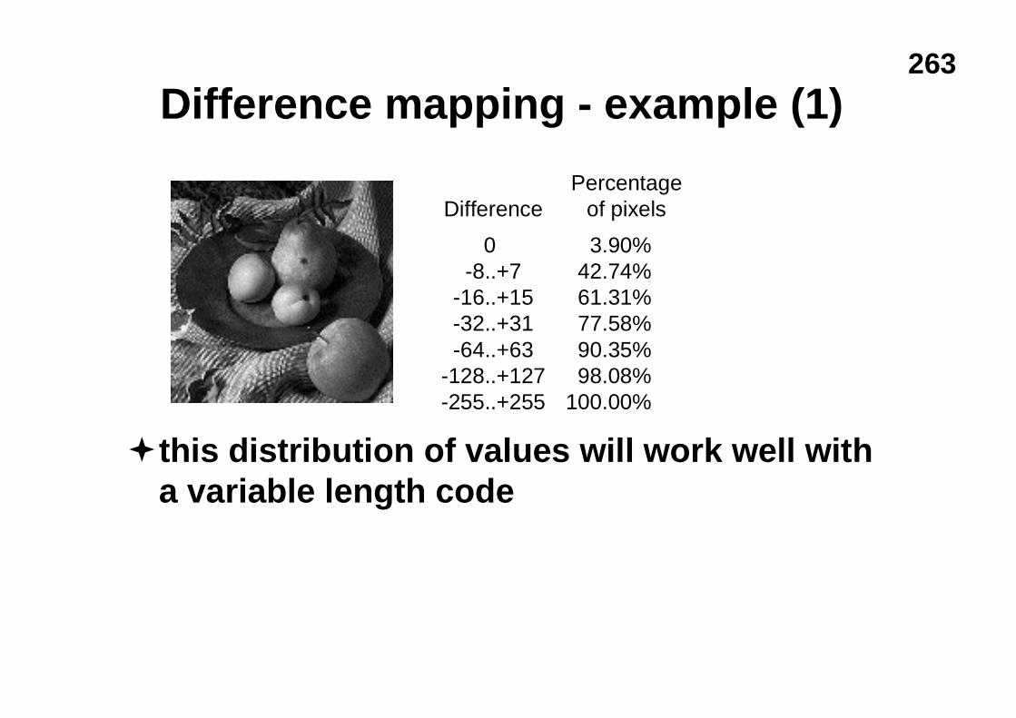
263

Difference mapping - example (1)

DifferencePercentage

of pixels

0 3.90%-8..+7 42.74%

-16..+15 61.31%-32..+31 77.58%-64..+63 90.35%

-128..+127 98.08%-255..+255 100.00%

�this distribution of values will work well witha variable length code

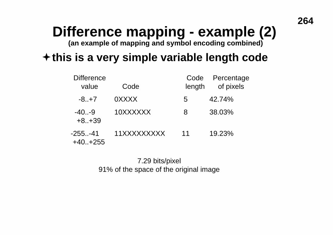
264Difference mapping - example (2)

-8..+7 0XXXX 5 42.74%

-40..-9 10XXXXXX 8 38.03%+8..+39

-255..-41 11XXXXXXXXX 11 19.23%+40..+255

7.29 bits/pixel91% of the space of the original image

Differencevalue Code

Codelength

Percentageof pixels

�this is a very simple variable length code(an example of mapping and symbol encoding combined)

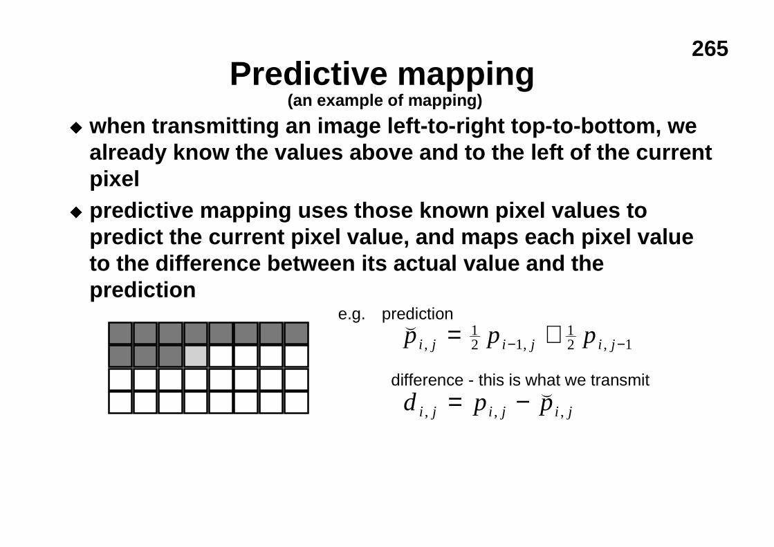
265Predictive mapping

u when transmitting an image left-to-right top-to-bottom, wealready know the values above and to the left of the currentpixel

u predictive mapping uses those known pixel values topredict the current pixel value, and maps each pixel valueto the difference between its actual value and theprediction

e.g. (p p pi j i j i j, , ,= +− −12 1

12 1

prediction

difference - this is what we transmit

d p pi j i j i j, , ,= − (

(an example of mapping)

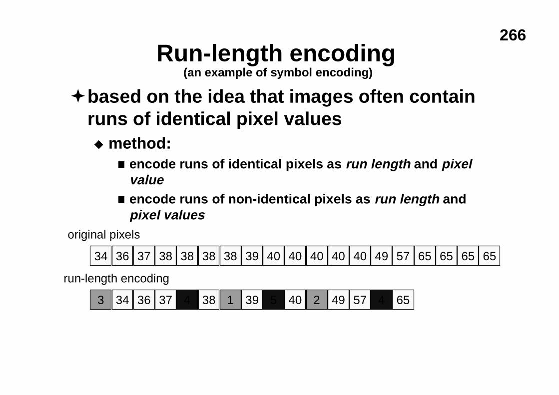
266Run-length encoding

�based on the idea that images often containruns of identical pixel valuesu method:

n encode runs of identical pixels as run length and pixelvalue

n encode runs of non-identical pixels as run length andpixel values

34 36 37 38 38 38 38 39 40 40 40 40 40 49 57 65 65 65

34 36 37 38 39 40 49 57 653 4 1 5 2 4

65

original pixels

run-length encoding

(an example of symbol encoding)

267

Run-length encoding - example (1)u run length is encoded as an 8-bit value:

n first bit determines type of runl 0 = identical pixels, 1 = non-identical pixels

n other seven bits code length of runl binary value of run length - 1 (run length ∈{1,…,128})

u pixels are encoded as 8-bit values

u best case: all runs of 128 identical pixelsn compression of 2/128 = 1.56%

u worst case: no runs of identical pixelsn compression of 129/128=100.78% (expansion!)

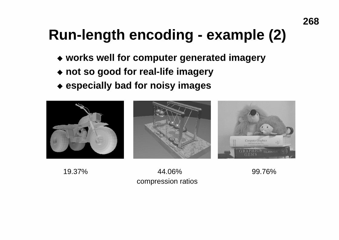
268

Run-length encoding - example (2)u works well for computer generated imageryu not so good for real-life imageryu especially bad for noisy images

19.37% 44.06% 99.76%compression ratios

269

CCITT fax encoding

�fax images are binary�1D CCITT group 3

u binary image is stored as a series of run lengthsu don’t need to store pixel values!

�2D CCITT group 3 & 4u predict this line’s runs based on previous line’s

runsu encode differences

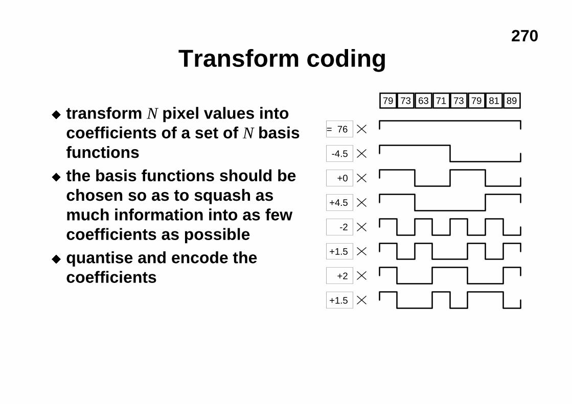
270

Transform coding

-4.5

= 76

+4.5

+0

+1.5

-2

+1.5

+2

79 73 63 71 73 79 81 89

u transform N pixel values intocoefficients of a set of N basisfunctions

u the basis functions should bechosen so as to squash asmuch information into as fewcoefficients as possible

u quantise and encode thecoefficients

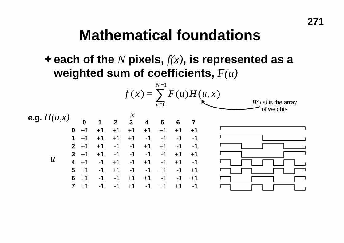
271

Mathematical foundations

�each of the N pixels, f(x), is represented as aweighted sum of coefficients, F(u)

f x F u H u xu

N

( ) ( ) ( , )==

−

∑0

1

0 1 2 3 4 5 6 70 +1 +1 +1 +1 +1 +1 +1 +11 +1 +1 +1 +1 -1 -1 -1 -12 +1 +1 -1 -1 +1 +1 -1 -13 +1 +1 -1 -1 -1 -1 +1 +14 +1 -1 +1 -1 +1 -1 +1 -15 +1 -1 +1 -1 -1 +1 -1 +16 +1 -1 -1 +1 +1 -1 -1 +17 +1 -1 -1 +1 -1 +1 +1 -1

e.g. H(u,x)

u

xH(u,x) is the array

of weights

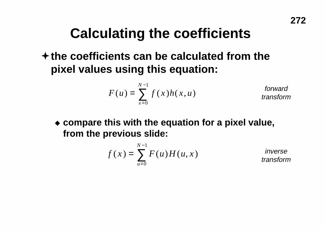
272

Calculating the coefficients

�the coefficients can be calculated from thepixel values using this equation:

u compare this with the equation for a pixel value,from the previous slide:

F u f x h x ux

N

( ) ( ) ( , )==

−

∑0

1

f x F u H u xu

N

( ) ( ) ( , )==

−

∑0

1

forwardtransform

inversetransform

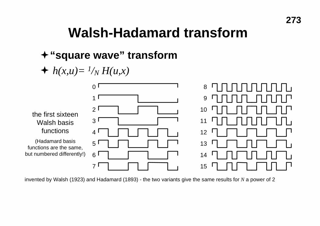
273

Walsh-Hadamard transform

�“square wave” transform� h(x,u)= 1/N H(u,x)

invented by Walsh (1923) and Hadamard (1893) - the two variants give the same results for N a power of 2

0

1

2

3

4

5

6

7

8

9

10

11

12

13

14

15

the first sixteenWalsh basis

functions(Hadamard basis

functions are the same,but numbered differently!)

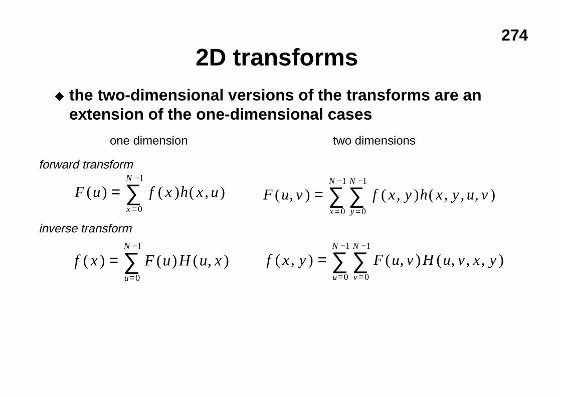
274

2D transformsu the two-dimensional versions of the transforms are an

extension of the one-dimensional cases

F u f x h x ux

N

( ) ( ) ( , )==

−

∑0

1

f x F u H u xu

N

( ) ( ) ( , )==

−

∑0

1

F u v f x y h x y u vy

N

x

N

( , ) ( , ) ( , , , )==

−

=

−

∑∑0

1

0

1

f x y F u v H u v x yv

N

u

N

( , ) ( , ) ( , , , )==

−

=

−

∑∑0

1

0

1

one dimension two dimensions

forward transform

inverse transform

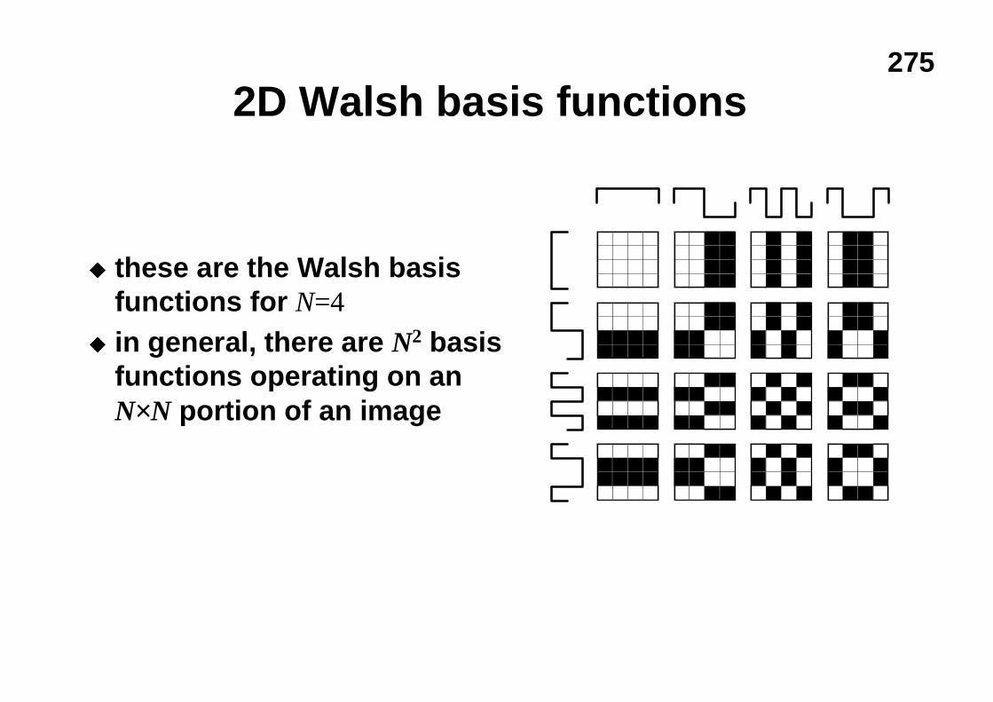
275

2D Walsh basis functions

u these are the Walsh basisfunctions for N=4

u in general, there are N2 basisfunctions operating on anN×N portion of an image

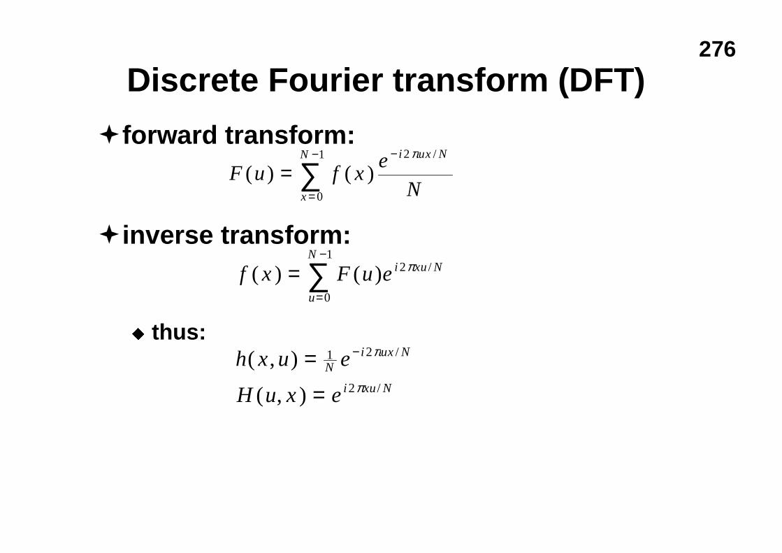
276

Discrete Fourier transform (DFT)

�forward transform:

�inverse transform:

u thus:

F u f xe

N

i ux N

x

N

( ) ( )/

=−

=

−

∑2

0

1 π

f x F u e i xu N

u

N

( ) ( ) /==

−

∑ 2

0

1π

h x u e

H u x e

Ni ux N

i xu N

( , )

( , )

/

/

=

=

−1 2

2

π

π

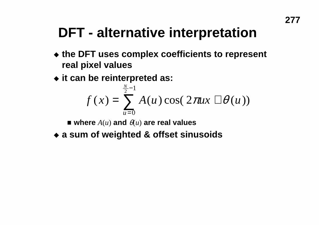
277

DFT - alternative interpretationu the DFT uses complex coefficients to represent

real pixel valuesu it can be reinterpreted as:

n where A(u) and θ(u) are real values

u a sum of weighted & offset sinusoids

∑−

=

+=1

0

2

))(2cos()()(N

u

uuxuAxf θπ

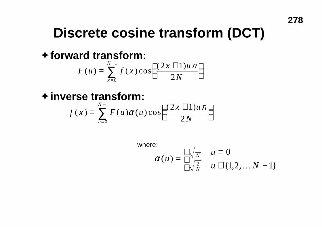
278

Discrete cosine transform (DCT)

�forward transform:

�inverse transform:

F u f xx u

Nx

N

( ) ( ) cos( )= +

=

−

∑ 2 120

1 π

f x F u ux u

Nu

N

( ) ( ) ( ) cos( )= +

=

−

∑ α π2 120

1

where:

α ( ){ , , }

uu

u NN

N

==∈ −

1

2

0

1 2 1K

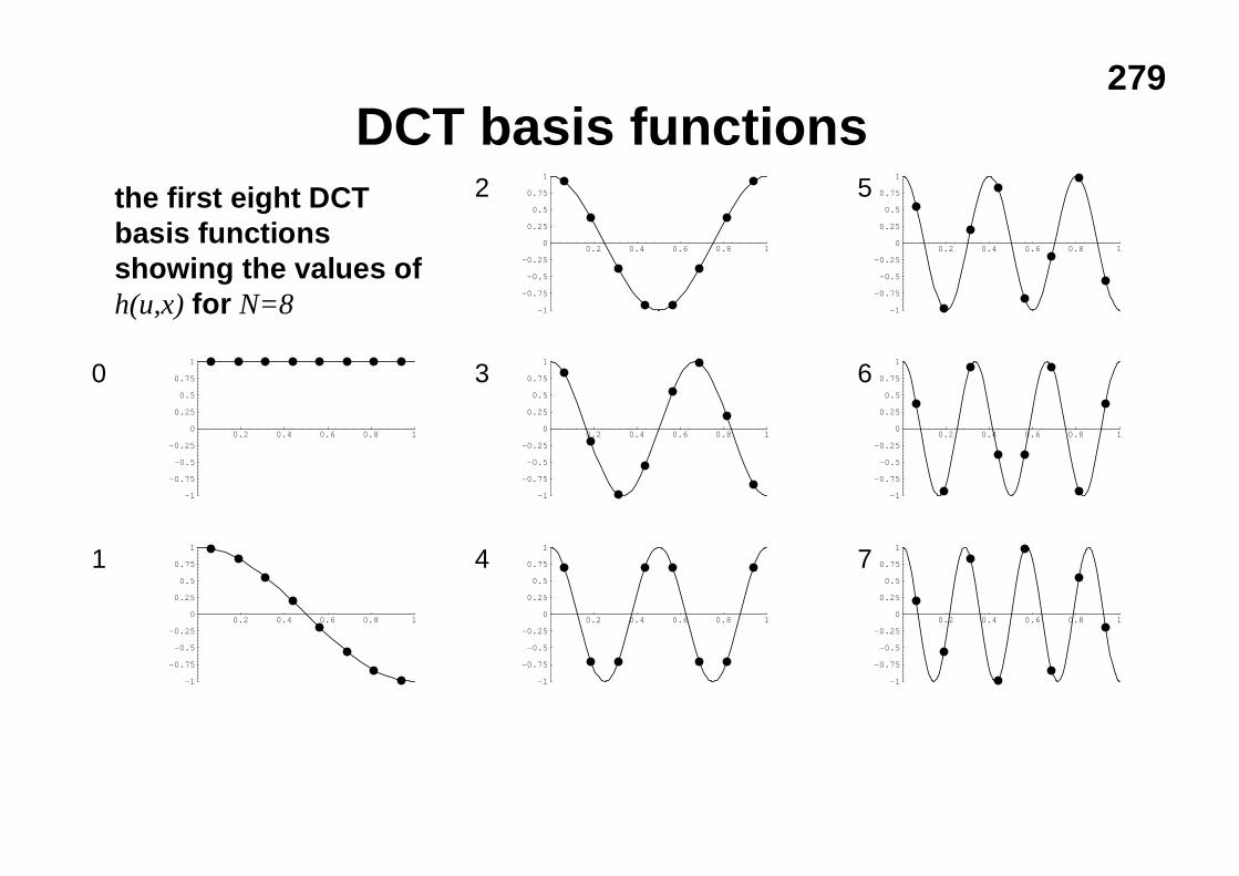
279

DCT basis functionsthe first eight DCTbasis functionsshowing the values ofh(u,x) for N=8

0.2 0.4 0.6 0.8 1

-1

-0.75

-0.5

-0.25

0

0.25

0.5

0.75

1

0.2 0.4 0.6 0.8 1

-1

-0.75

-0.5

-0.25

0

0.25

0.5

0.75

1

0.2 0.4 0.6 0.8 1

-1

-0.75

-0.5

-0.25

0

0.25

0.5

0.75

1

0.2 0.4 0.6 0.8 1

-1

-0.75

-0.5

-0.25

0

0.25

0.5

0.75

1

0.2 0.4 0.6 0.8 1

-1

-0.75

-0.5

-0.25

0

0.25

0.5

0.75

1

0.2 0.4 0.6 0.8 1

-1

-0.75

-0.5

-0.25

0

0.25

0.5

0.75

1

0.2 0.4 0.6 0.8 1

-1

-0.75

-0.5

-0.25

0

0.25

0.5

0.75

1

0.2 0.4 0.6 0.8 1

-1

-0.75

-0.5

-0.25

0

0.25

0.5

0.75

1

0

1 4

3

2

7

6

5

280

Haar transform: waveletsu “square wave” transform, similar to Walsh-

Hadamardu Haar basis functions get progressively more local

n c.f. Walsh-Hadamard, where all basis functions are global

u simplest wavelet transform

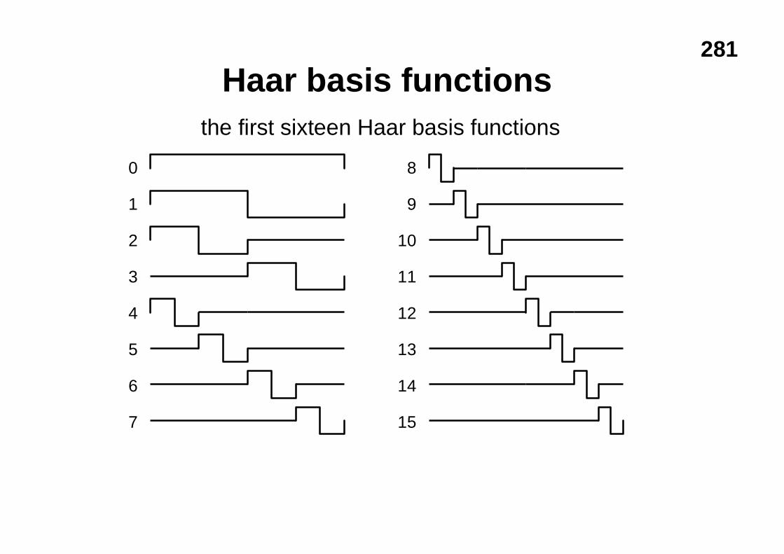
281

Haar basis functions

0

1

2

3

4

5

6

7

8

9

10

11

12

13

14

15

the first sixteen Haar basis functions

282

Karhunen-Loève transform (KLT)“eigenvector”, “principal component”, “Hotelling” transform

�based on statistical properties of the imagesource

�theoretically best transform encoding method�but different basis functions for every

different image source

first derived by Hotelling (1933) for discrete data; by Karhunen (1947) and Loève (1948) for continuous data

283

JPEG: a practical example

�compression standardn JPEG = Joint Photographic Expert Group

�three different coding schemes:u baseline coding scheme

n based on DCT, lossyn adequate for most compression applications

u extended coding schemen for applications requiring greater compression or higher

precision or progressive reconstruction

u independent coding schemen lossless, doesn’t use DCT

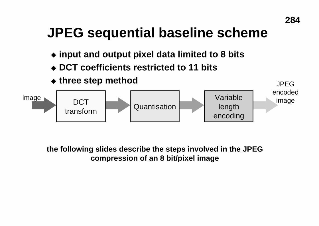
284

JPEG sequential baseline schemeu input and output pixel data limited to 8 bitsu DCT coefficients restricted to 11 bitsu three step method

DCTtransform

QuantisationVariablelength

encoding

image

JPEGencodedimage

the following slides describe the steps involved in the JPEGcompression of an 8 bit/pixel image

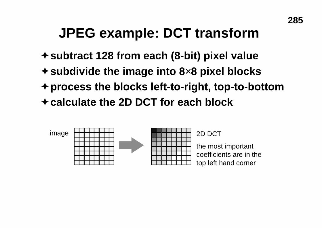
285

JPEG example: DCT transform

�subtract 128 from each (8-bit) pixel value�subdivide the image into 8×8 pixel blocks�process the blocks left-to-right, top-to-bottom�calculate the 2D DCT for each block

image 2D DCT

the most importantcoefficients are in thetop left hand corner

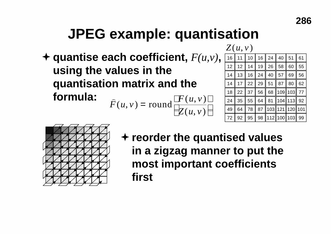
286

JPEG example: quantisation

�quantise each coefficient, F(u,v),using the values in thequantisation matrix and theformula: )

F u vF u v

Z u v( , )

( , )( , )

=

round

� reorder the quantised valuesin a zigzag manner to put themost important coefficientsfirst

16 11 10 16 24 40 51 61

12 12 14 19 26 58 60 55

14 13 16 24 40 57 69 56

14 17 22 29 51 87 80 62

18 22 37 56 68 109 103 77

24 35 55 64 81 104 113 92

49 64 78 87 103 121 120 101

72 92 95 98 112 100 103 99

Z u v( , )

287

JPEG example: symbol encoding

�the DC coefficient (mean intensity) is codedrelative to the DC coefficient of the previous 8×8block

�each non-zero AC coefficient is encoded by avariable length code representing both thecoefficient’s value and the number of precedingzeroes in the sequenceu this is to take advantage of the fact that the sequence

of 63 AC coefficients will normally contain long runsof zeroes