1 Complex Numbers in Quantum Mechanics

Complex numbers and variables can be useful in classical physics. However, theyare not essential. To emphasize this, recall that forces, positions, momenta, potentials,electric and magnetic fields are all real quantities, and the equations describing them,Newton’s laws, Maxwell’s equations,etc. are all differential equations involving strictlyreal quantities.

Quantum mechanics is different. Factors of i =√−1 are everywhere, for example

from Heisenberg we have his famous commutation relation,

QP − PQ = ih,

and from Schrodinger his equally famous equation

h

i∂tΨ = HΨ.

The wave function Ψ is complex and so is practically every other quantity neededto formulate quantum mechanics. Granted that classical mechanics fails at distancesof nanometer or less, why is it suddenly so necessary that everything be complex?

Comment 1 An interesting question is the distance scale below whicha quantum treatment is essential. A nanometer seems like a reasonablechoice. But even more intriguing is the question of what happens onmuch bigger scales, centimeters, meters, and larger. Does quantummechanics still govern things, or does it somehow break down? In2011, it is fair to say no definite answer to this question is known.

Returning to the question of why quantum mechanics requires complex quantities,one reason becomes apparent upon trying to describe wavelike phenomena for materialparticles, electrons, neutrons, etc. To see this point, start with a classical electromagneticwave. For a plane wave traveling along the z−axis, we can write the following formulafor the electric field,

E = E0x cos(kz − ωt). (1)

To be more realistic, we should of course superpose nearby frequencies so that the wavehas a finite extent. However, the observation we will make applies equally well whether wehave a single frequency or a superposition of a narrow range of frequencies. For simplicity,we will use the simple formula Eq.(1). We may break Eq.(1) into pure exponentials ,so-called “positive frequency” and “negative frequency” parts;

E = E0x(e−iωt+ikx + eiωt−ikx).

(By long-established convention exp(−iωt) is taken to be the positive frequency part(ω > 0 here), and exp(+iωt) is the negative frequency part.) The important point is that

1

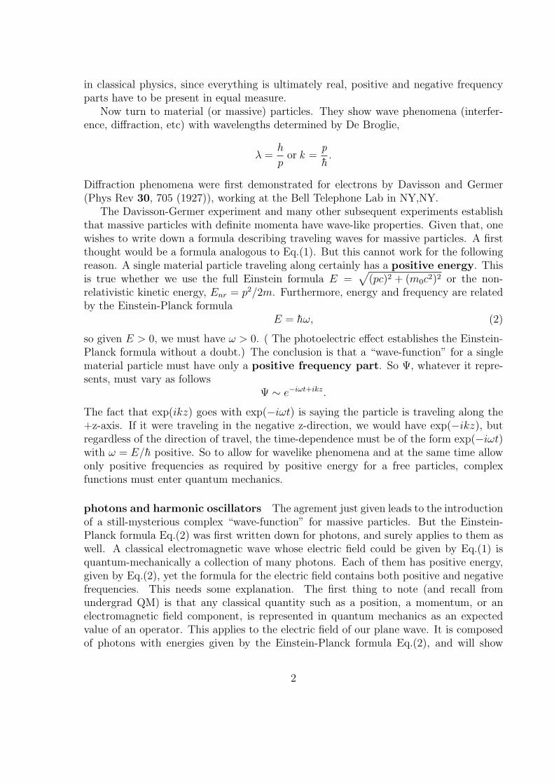
in classical physics, since everything is ultimately real, positive and negative frequencyparts have to be present in equal measure.

Now turn to material (or massive) particles. They show wave phenomena (interfer-ence, diffraction, etc) with wavelengths determined by De Broglie,

λ =h

por k =

p

h.

Diffraction phenomena were first demonstrated for electrons by Davisson and Germer(Phys Rev 30, 705 (1927)), working at the Bell Telephone Lab in NY,NY.

The Davisson-Germer experiment and many other subsequent experiments establishthat massive particles with definite momenta have wave-like properties. Given that, onewishes to write down a formula describing traveling waves for massive particles. A firstthought would be a formula analogous to Eq.(1). But this cannot work for the followingreason. A single material particle traveling along certainly has a positive energy. Thisis true whether we use the full Einstein formula E =

√(pc)2 + (m0c2)2 or the non-

relativistic kinetic energy, Enr = p2/2m. Furthermore, energy and frequency are relatedby the Einstein-Planck formula

E = hω, (2)

so given E > 0, we must have ω > 0. ( The photoelectric effect establishes the Einstein-Planck formula without a doubt.) The conclusion is that a “wave-function” for a singlematerial particle must have only a positive frequency part. So Ψ, whatever it repre-sents, must vary as follows

Ψ ∼ e−iωt+ikz.

The fact that exp(ikz) goes with exp(−iωt) is saying the particle is traveling along the+z-axis. If it were traveling in the negative z-direction, we would have exp(−ikz), butregardless of the direction of travel, the time-dependence must be of the form exp(−iωt)with ω = E/h positive. So to allow for wavelike phenomena and at the same time allowonly positive frequencies as required by positive energy for a free particles, complexfunctions must enter quantum mechanics.

photons and harmonic oscillators The agrement just given leads to the introductionof a still-mysterious complex “wave-function” for massive particles. But the Einstein-Planck formula Eq.(2) was first written down for photons, and surely applies to them aswell. A classical electromagnetic wave whose electric field could be given by Eq.(1) isquantum-mechanically a collection of many photons. Each of them has positive energy,given by Eq.(2), yet the formula for the electric field contains both positive and negativefrequencies. This needs some explanation. The first thing to note (and recall fromundergrad QM) is that any classical quantity such as a position, a momentum, or anelectromagnetic field component, is represented in quantum mechanics as an expectedvalue of an operator. This applies to the electric field of our plane wave. It is composedof photons with energies given by the Einstein-Planck formula Eq.(2), and will show

2

classical behavior if many photons are present. The numerical value of the electric fieldwill be the expected value of an electric field operator. You will learn how to handle thisoperator later in the course, but in the end, the electromagnetic field is nothing but abunch of harmonic oscillators. So we can study the point about positive and negativefrequencies by examining a simple harmonic oscillator. Classically, we can write

x(t) = Ae−iωt + Aeiωt. (3)

In quantum mechanics, x(t) will be the expected value of the position operator x, writtenas < x(t) >. ( We are abusing notation by using the same symbol for the classical positionand the quantum operator. This is common practice in physics.) Since the expected valueis real, certainly both positive and negative frequencies appear, just as in Eq.(3).

Summary The really important points of the above discussion are: (1) Einstein andPlanck have taught us that energy and frequency are proportional, the proportionalityconstant being Planck’s constant. (2) Energy is not like momentum where positive andnegative values both occur equally. The energy of any system has a lower bound andallowed energies go up from there. So it is natural when we write a quantity that variesas ∼ exp(−iωt), that we will not always have a balancing term the varies as ∼ exp(iωt),although this will happen when we are examining an expected value of an operator. Sincecomplex conjugates are bound to occur, there will also be cases where terms ∼ exp(+iωt)do not have a balancing ∼ exp(−iωt). Bottom line: In quantum mechanics, complexnumbers are essential.

2 Photon Polarization, Probability and Interference

in Quantum Mechanics

The existence of polarized light gives a wonderful example where both classical ideas andone of the most puzzling features of quantum mechanics coexist. Polarization is veryfamiliar in daily life. Almost everyone who wears sunglasses wears polarized sunglasses,which are designed to absorb horizontally polarized light. This can be experienced at thelocal gas station when you fill your gas tank. If you are wearing polarized sunglasses, youwill quickly discover that the light emitted by the display on the gas pump is polarized.For those who do not operate cars, try putting on your polarized sunglasses the nexttime you are in front of a computer monitor. Tilting your head reveals that the lightfrom the monitor is highly polarized.

Let us start by discussing a classical beam of monochromatic light, traveling alongthe +z axis. Imagine we have ideal polarizer placed in this beam with its axis along the+y axis. This means that light polarized along y is (ideally) 100% transmitted, whilelight polarized along the x axis is totally absorbed. Now if the incident light is polarizedat say an angle θ with respect to the y axis, we simply resolve the polarization into a

3

component along the y axis, and one along the x axis. Only the component along the yaxis gets transmitted, and the transmitted intensity satisfies the classical Malus Law:

I(θ) = I(0) cos2 θ, (4)

where I(θ) is the intensity of transmitted light, when the incident light is polarized atangle θ to the axis of the polarizer. This is all well-known seemingly pure classical physics.

Now Malus’ law puts no restriction on the intensity of the incident light. So imaginethat we gradually but steadily reduce the intensity to the point where we are consideringthe process photon by photon. At this point quantum physics enters the picture, but onlyin a very general way. We visualize a classical light beam as composed of photons, eachsatisfying the Einstein-Planck formula relating frequency and energy. For this discussion,we don’t need this formula. All we do need is the assertion that photons cannot be brokeninto pieces, only whole photons are observed beyond the polarizer. Now as long as thephoton’s polarization vector is either along y, or along x, there is still no need for newideas. The photon polarized along y gets transmitted, the one polarized along x getsabsorbed. New ideas do enter when we have a photon incident whose polarization vectoris at angle θ with respect to y. A polarization vector for an individual photon is a unitvector, which we could write for our present discussion as

P = cos θy + sin θx. (5)

This is the polarization vector of the photon which is incident on the polarizer. Beyondthe polarizer, there either a photon or no photon. If there is a photon, its polarizationvector is y. When this experiment is repeated over and over, always with the samepolarization for the incident photon, the frequency of observation of photons transmittedbeyond the polarizer is cos2 θ. Whether a given photon is transmitted is apparentlyrandom. Large numbers of observations are needed to observe the cos2 θ law. Thisis indeed something new and unfamiliar at the macroscopic level. To interpret thisresult requires the introduction of probability into quantum mechanics. In our example,probability is invoked as follows. We know that if the photon polarization is along y, thephoton is transmitted, while if its polarization is along x, it is absorbed. We say that theprobability amplitude of our photon being found with its polarization along y is

y · P = cos θ, (6)

and the probability of the photon being found with polarization along y is the absolutesquare of the probability amplitude. Denoting this probability as py, we can write

py = |y · P |2 (7)

Note that we did not need the absolute value in Eq.(7). However, probability amplitudesare complex in general, so to get a real probability, it is necessary to take the absolutesquare of the probability amplitude. Eq.(7) allows us to explain the experiment in astatistical sense. No answer can be given to the question of what transpires for an

4

individual photon. Answers can only be given to questions involving many repeats of theexperiment. At this level, quantum probability is like coin-tossing. One cannot say whatthe outcome will be for a toss of an individual coin. Many tosses are needed to see thatthe chance of “heads” is 0.50 for an unbiased coin. The idea of “hidden” variables inquantum mechanics can be explained using coin tosses. While we say that the outcomeof a coin toss is random, if we were willing to undertake the enormous task of solvingthe equations of motion taking account of all possible forces and carefully specifying theinitial conditions, the outcome of a coin toss is predictable. In the same way, so-calledhidden variable theories of quantum behavior postulate the existence of subtle or hiddenvariables, whose consideration would allow the apparent randomness of outcomes to beunderstood as not really random after all. Hidden variable theories have had a difficulttime and it is safe to say that no real evidence exists that any of the ones proposed sofar can accomplish the task of taking the probability out of quantum mechanics. We areleft with the situation that the probabilities we have in quantum mechanics are reallyintrinsic, and there is no deeper level at which there are new variables which if treatedwould remove randomness. It is well-known that this intrinsic nature of probability inquantum mechanics was bothersome to some very great physicists. Einstein is the mostfamous example, but Schrodinger also had serious reservations, some of which have beenignored rather than answered.

Given that there is no working alternative, let us go on to state more clearly thesituation with respect to probability in quantum mechanics. To warm up, there are somecomments that can be made about our polarized photon example. First note that noenergy is getting lost. The incident photon either goes through or is absorbed. If it isabsorbed, the energy of the photon is given to the absorbing material. That is fairlyobvious. The polarization experiment is really a scattering experiment, elastic scatteringfor the transmitted photon, inelastic for the absorbed photon. Experiments involvingscattering often give clear examples of quantum probability. Second, note that we werecareful to discuss the polarization of the photon, not its electric field. Classically we thinkof the polarization is simply the direction of the electric field of the wave. This is fine if wehave many photons and in fact an indefinite number of photons. However, at the singlephoton level, there is no “value” of the electric field. As we will see later, the electricfield operator is non-diagonal in photon number. Nevertheless, the polarization of anindividual photon makes perfect sense. It is a unit vector, perpendicular to the directionof wave propagation. Note that dotting two ordinary vectors does not lead to a quantitywhose square could be a probability. However, if they are unit vectors, a probabilityinterpretation is possible. The introduction of probability into quantum mechanics wasmainly the work of Max Born, who reasoned from the results of scattering experiments.

5

Probability in Quantum Mechanics

Now we can state the way probability comes into quantum mechanicsin a rather general way. Note that this is a huge extrapolation from ourphoton polarization example, but it nevertheless fits all known experi-ence. First the notion of quantum state. A quantum state is a vectorin a complex vector space, possibly one of an infinite number of di-mensions. Call the vector u. Now suppose there is another state of oursystem, described by a different vector v. Generalizing the discussion inthe photon case, it is necessary that these both be unit vectors, so ourspace needs to have a notion of length for its vectors. Next, to defineprobability amplitudes, we need to be able to take the “dot” or innerproduct of two vectors, denoted as (v,u), so our space needs to be aninner product space. Finally, if the state is u, the probability that it isfound to be in v is |(v,u)|2, i.e. the absolute square of the probabilityamplitude.

• Quantum State ←→ v, a unit vector in a complex space.

• Probability Amplitude = (v,u), the amplitude to find state v ina known state u.

• Probability = |(v,u)|2, the probability to find state v in a knownstate u.

Interference and Superposition in Quantum Mechanics So far we have usedthe polarization of photons as a vehicle for understanding how probability comes intoquantum mechanics in an essential way. We could use photon polarization for a discussionof interference as well. However, there are more familiar examples. Interference is reallya hallmark of wave phenomena. Waves arriving at a given point via different pathsmay add up or cancel each other out. Young’s two slit experiment, the behavior ofdiffraction gratings, etc are familiar examples from classical physics with light. Manymore examples can be given in classical physics, most notably from acoustics. TheDavisson-Germer experiment demonstrated for the first time that interference can happenfor material particles like electrons. This means that when an electron of reasonablywell-defined momentum enters a crystal and then leaves again, there can be maxima andminima observed between electron waves arriving at a given point via different paths.Amplitudes may add constructively or destructively. We have said already that to evendescribe waves for material particles, we need complex quantities. Since interferenceinvolves superposition, adding such quantities must give a quantity of the same type.More formally it is essential that when we add (superpose) objects representing states,we get other objects representing states, and here superposition involves not just additionbut addition and multiplication with complex numbers.

6

Superposition in Quantum Mechanics

A quantum state is a vector in a complex vector space, possibly oneof an infinite number of dimensions. Call the vector u. Now supposethere is another state of our system, described by a different vector v.The idea of superposition states that combining these vectors as in

w = αv + βv (8)

must give another vector w, which when normalized, is a possible stateof the system. (Here α and β are complex numbers.) This is maximallyweird when thought of in terms of classical particle physics. Addingtwice one state of a particle to 1/10 of another state of the particle toget a third state of the particle? No way in classical physics. But it isabsolutely required by experiment in quantum physics!

The next sections will go into some of the features of complex vector spaces in detail.

3 Complex Vectors

Let us start with an ordinary vector in three-dimensional space, as used in elementaryphysics. We usually expand such a vector in an orthonormal basis,

v = v1e1 + v2e2 + v3e3, (9)

where the ei are orthogonal unit vectors, and the vi are real scalars (not vectors), calledthe components of v. For the words orthogonal and unit vector to make sense theremust be a scalar or inner product. In elementary physics we write this as a “dotproduct”,

ei · ej = δij. (10)

For our work in quantum mechanics, a different notation will be essential. So for thescalar product of ei with ej, we write (ei, ej). (Later, we will also use < ei, ej > and< ei|ej > to mean the same thing.) Apart from notation, certain generalizations ofordinary 3-vectors are necessary. First, since our quantum vectors reside generally in thespace of quantum states, the dimensionality of the space will usually not be three. Wewill work in n dimensions, where n = 2, 3, . . ., including spaces of an infinite number ofdimensions. Second, having seen that quantummechanics must involve complex numbers,the components of vectors must be allowed to be complex numbers. The scalar productis also naturally generalized. The scalar product of a vector v with a vector u will bedenoted as (v,u). This is a complex number, defined so that

(v,u) = (u,v), (11)

7

where a bar over a quantity means complex conjugate. As far as unit vectors are con-cerned, we still have

(ei, ej) = (ej, ei) = δij, (12)

but for more general vectors, it does matter which vector is on the right or the left in(v,u). The physics convention is that (v,u) is linear in u and antilinear in v. Let usillustrate with a simple example. Suppose u = αej, and v = βek, where α and β arearbitrary complex numbers. Then by linearity

(v,u) = (v, αej) = α(v, ej), (13)

and by anti-linearity(v, ej) = (βek, ej) = β(ek, ej), (14)

so we would get(v,u) = βα(ek, ej) = (βα) δkj. (15)

Now consider a less trivial example. Suppose our space has n dimensions, so u and vcan be expanded as

u =n∑

j=1

ujej (16)

v =n∑

k=1

vkek

The scalar product of v and u is

(v,u) = (∑k

vkek,∑j

ujej) =∑k,j

vkuj(ek, ej) =∑j

vjuj (17)

It is obvious from this equation that (v,v) ≥ 0 so for any non-zero vector v, we candefine its norm by

||v|| =√

(v,v). (18)

An application of our formulas so far is to prove the Schwarz inequality, which statesthat

|(v,u)| ≤ ||v|| · ||u||, (19)

for any two vectors u and u. Rearranging the formula Eq.(19), we can write it as

|(ev, eu)| ≤ 1, (20)

whereev =

v

||v||(21)

andeu =

u

||u||

8

are unit vectors.

Exercise 2 To prove the Schwarz inequality in the form of Eq.(20),consider the vector w = αev + 1

αeu, where α is a complex number.

Eq.(20) may be proven by demanding that (w,w) ≥ 0, and choosingthe magnitude and phase of α appropriately.

Linear Independence and Bases The notion of linear independence is a simplebut useful one. Suppose our space has n dimensions, and that we have n vectors{b1,b2, . . . ,bn}. This set is linearly independent if any vector in the space can be writtenas

u =n∑

j=1

ujbj. (22)

Said another way, there are n linearly independent vectors in an n dimensional space.Any such set of n linearly independent vectors is called a basis. As a simple example oflinear independence, think of ordinary 3 dimensional space. Pick any vector in the spacefor b1, then pick a second vector not parallel to b1 for b2. All possible vectors composedof b1 and b2 compose a plane. Pick a third vector b3 which does not lie totally in thatplane. Then b1,b2, and b3 are a set of linearly independent 3-vectors and form a basisfor 3 dimensional space.

Orthogonalization Once we have a basis, we can find the components of a vector.From Eq.(22) we have

(bk,u) =n∑

j=1

uj(bk,bj), (23)

so we can solve for the uj by solving n equations in n unknowns. Although perfectlypossible, this is certainly not a convenient procedure. It is much more convenient tohave an orthonormal basis. Orthogonalization (or the Gram-Schmidt procedure ) is amethod for constructing an orthonormal basis {e1, e2, . . . , en} from an arbitrary basis{b1,b2, . . . ,bn}. Start by defining

e1 =b1

||b1||.

Next set h2 = b2 − e1(e1,b2). This removes the part of b2 along e1. Then set

e2 =h2

||h2||.

9

The process continues by setting h3 = b3 − e1(e1,b3) − e2(e2,b3), which removes thepart of b3 along e1 and e2. Then set

e3 =h3

||h3||,

and so on.

Hilbert Space A Hilbert space H is (roughly) the limit as n → ∞ of our discussionup to now. The example closest to our previous discussion is called l2. In this space,a vector is just a infinite list of components. The scalar product of vectors u and v isnaturally written as the limit of Eq.(17),

(u,v) =∞∑j=1

ujvj, (24)

where to be elements of the space at all both

(v,v) =∞∑j=1

vjvj, (25)

and

(u,u) =∞∑j=1

ujuj, (26)

must be finite. We may define the orthonormal basis of this space by the followingequations

e1 = {1, 0, 0, . . .}, (27)

e2 = {0, 1, 0, . . .},e3 = {0, 0, 1, . . .},

. . . . . . . . . . . . ,

which clearly defines an infinite set of linearly independent vectors.In order to be mathematically well-defined a Hilbert space H needs to obey certain

extra conditions. We will assume that our Hilbert spaces are all “nice” and do obeythese requirements. For the record they are called completeness and separability. Thefollowing is a rough description of these. Once we have a scalar product, we can definethe norm of a vector, see Eq.(18). The distance between two vectors is then defined asthe norm of the difference,

D(u,v) = ||u− v|| (28)

Now suppose we have a sequence of vectors un such that

D(un,um)→ 0,

10

as m,n → ∞. This says the members of the sequence are getting closer and closertogether. Now are they getting close to a vector that is the limit of the sequence? If sothe space is complete. This is very analogous to the relationship of rational numbers toirrational numbers. The requirement of separability is as follows. There is a countableset of vectors in H such that for any vector u in H, we can find a member of the set g,such that D(u,g) < ϵ for any small ϵ. This requirement holds for all the spaces used inordinary quantum mechanics, and we need not consider it explicitly any further.

Another example We have mentioned the Hilbert space l2. A second example isL2, the space of square integrable functions on an interval, perhaps infinite in length.A simple but important case is square integrable functions on the interval (0, 2π). Thescalar product is

(u,v) =

∫ 2π

0

u(x )v(x )dx . (29)

An orthonormal basis for L2(0, 2π) is the set of functions

1√2π

exp(ikx) (±k = 0, 1, 2, . . .). (30)

We may establish a correspondence between the vectors in the abstract sense and theirrealization as functions in L2(0, 2π),

v ↔ v(x ) (31)

ek ↔1√2π

exp(ikx )

This space is important and we will work with it more later on.

Comment 2 An eternal question in any advanced part of physics ishow much math is needed? In the case of Hilbert space, a great dealhas been worked out, much of it by John von Neumann in a series ofpapers written in the 1920’s and his famous book, “The MathematicalFoundations of Quantum Mechanics”. However, few physicists have thetime or the inclination to delve into the technicalities of Hilbert spaceor other mathematical subjects that deeply. A reasonable attitude isto make sure the physics equations written down are understood andmake sense. Physics arguments can often be used to settle fine points.A quote from Feynman on higher mathematics is “Don’t know howto prove what’s true. Just know what’s true!” We will try tofollow this suggestion.

11

4 Operators and Adjoints

An operator is a rule generating a vector in our space by acting on an original vector.We will only need to consider linear operators, so if T is an operator, we have

T (αu1 + βu2) = αTu1 + βTu2. (32)

Generally speaking, in quantum mechanics, operators either represent physical quantitieslike momentum, energy, angular momentum, or represent transformations like rotations,translations, Lorentz transformations, or simple changes of coordinate system in ourcomplex space.

An important concept for a linear operator T is its adjoint, denoted as T †. Thedefining property of the adjoint of an operator is

(u,Tv) = (T†u,v) (33)

To get used to the concept of adjoint, let us look at an example using a orthonormalbasis. Our space can be finite- or infinite-dimensional. We will assume all infinite sumsconverge. Let

u =∑j

ujej (34)

Acting on u with T , we have

Tu =∑j

ujTej. (35)

Now Tej can be expanded in our space, so we can write

Tej =∑k

ektkj, (36)

The peculiar way terms are written in Eq.(36) becomes clearer when we take matrixelements of T. We have

(ek,Tej) = tkj, (37)

where tkj are a set of numbers, complex in general.NOTE: Physics notation often uses the same letter to denote several different things.

We will do this eventually, but for now, we are trying to distinguish the operator T fromits matrix elements in an orthonormal basis, (ej,Tek), so we use tjk to denote themrather than Tjk.

Turning to the adjoint of T , by analogy with Eq.(36) we may write

T †ej =∑k

ektkj, (38)

where the tkj are another arbitrary set of complex numbers. Taking matrix elements, wehave

(ek,T†ej) = tkj, (39)

12

so the tkj are the matrix elements of T †. Computing T †u we have

T †u =∑j

ujT†ej =

∑k,j

ektkjuj. (40)

Substituting this into (T †u,v) we have

(T †u,v) = (∑k,j

ujektkj ,∑m

vmem) =∑k,j

uj(tkj)∗vk. (41)

Now consider (u,Tv). An easy calculation gives

(u,Tv) =∑k,j

ujtjkvk. (42)

By definition, (u,Tv) = (T†u,v). Further, u and v are arbitrary vectors in our space,so from Eqs.(40) and (42) we must have

(tkj)∗ = tjk (43)

A more illuminating form for this equation follows when we use Eqs.(37) and (39). Usingthose equations, Eq.(43) becomes

(ek,T†ej)

∗ = (ej,Tek). (44)

At this point, let us revert to standard physics notation, and write

(ej,Tek) = Tjk (45)

(ej,T†ek) = T†

jk,

and Tjk = (T †kj)

∗. Now if write T out as a matrix array Tjk (this called “defining an

operator by its matrix elements”), then the matrix for T † or T †jk is just the adjoint in

the matrix sense of the matrix for T. (Recall that the matrix adjoint operation takes thecomplex conjugate of every element and replaces the resulting matrix by its transpose.)

Self-Adjoint and Unitary Operators The two most important classes of operatorsused in quantum mechanics are self-adjoint (or Hermitian) operators, and unitary oper-ators. A self-adjoint operator is one for which the adjoint is the same as the operator,

T † = T. (46)

Self-adjoint operators correspond to physical quantities like energy, momentum, etc. Letus consider the eigenvalue of a self-adjoint operator. Suppose T is self-adjoint, and thereis a vector u in our space such that

Tu = λu, (47)

13

where λ is a number called the eigenvalue. Consider the following matrix element,

(u,Tu) = λ(u,u). (48)

Now take complex conjugates of both sides,

(u,Tu)∗ = λ∗(u,u) (49)

Now by definition,(u,Tu)∗ = (Tu,u). (50)

Now use the fact that T is self-adjoint to get

(Tu,u) = (u,Tu) (51)

But now from Eqs.(48) and (49) we have

λ(u,u) = λ∗(u,u), (52)

which implies λ=λ∗, i.e. the eigenvalue is real. So self-adjoint operators have real eigen-values. (NOTE: The argument just given is fine for λ in the point or discrete spectrumof T. It needs extension for the case where T has a continuous spectrum. Remarks willbe made on this in a later section.)

Another characteristic property of self-adjoint operators has to do with multiple eigen-values. Suppose a self-adjoint operator T has two distinct eigenvalues: Tu = λu, andTv = µv. We have

(v,Tu) = λ(v,u) = (Tv,u) = µ(v,u). (53)

But this says(λ− µ)(v,u) = 0, (54)

so if λ = µ, we must have (v,u) = 0, so eigenvectors with different eigenvalues must beorthogonal.

Now let us consider unitary operators. The defining property of a unitary operatorU is

(v,u) = (Uv,Uu), (55)

i.e. U preserves the inner product of vectors. Now like any operator, U has a adjoint, sowe can write

(Uv,Uu) = (U†Uv,u). (56)

But using Eq.(55) we have(v,u) = (U †Uv,u). (57)

Now u and v were arbitrary vectors, so we must have

U †U = I (58)

14

i.e. for a unitary operator, the adjoint of the operator is its inverse. Considering theeigenvalues of a unitary operator, suppose

Uu = λu, (59)

where λ is a number. Now using the properties of unitary operators, we have

(Uu,Uu) = (λu, λu) = λ∗λ(u,u) = (u,u). (60)

which says λ∗λ = 1, i.e. the eigenvalues of a unitary operator are of the form exp(iθ).Again, this argument needs more work when dealing with the continuous spectrum.

Summary Self-adjoint operators have real eigenvalues. For a unitary operator, theadjoint is the inverse, and eigenvalues are complex numbers of unit modulus. Both ofthese results are true in general, although the discussion above has only covered the caseof eigenvalues in the discrete spectrum of the operator. For a self-adjoint operator, it isexpected that the eigenvectors will span the space, and any vector can be expanded inthese eigenfunctions. A simple example of this is Fourier series on the interval 0, 2π. Thegeneral expectation that an eigenfunction expansion exists is borne out in problems ofphysical interest.

Example Let us consider an example, chosen with an eye to physics applications. Wework in a three dimensional complex space, and define an operator J by

Je1 = ie2 (61)

Je2 = −ie1Je3 = 0

Exercise 3 Show that J is self-adjoint using the definitions of theprevious section.

We want to find eigenvalues and eigenvectors for J. Since we are in three dimension, weexpect three eigenvalues and corresponding eigenvectors. We will denote our normalizedeigenvectors as pλ, where λ is the eigenvalue. From Eq.(61), we have that e3 is aneigenvector with eigenvalue 0, so we write

e3 = p0 (62)

To find the other eigenvalues and eigenvectors, we apply J a second time. Using Eq.(61)we have

J(Je1) = iJe2 = e1 (63)

J(Je2) = −iJe1 = e2

Eq.(63) shows that for any vector in the subspace spanned by e1 and e2, the operatorJJ acts like the identity. Since the remaining eigenvectors reside in this space, we musthave λ2 = 1 for any eigenvalue. Let us try λ = −1. Expand e−1 as

p−1 = αe1 + βe2, (64)

15

where α and β are complex coefficients. Demanding that p−1 be an eigenvector of J witheigenvalue -1, we get

Jp−1 = αJe1 + βJe2 = iαe2 − iβe1 = −(αe1 + βe2). (65)

Matching coefficients of e1 and e2, we find that β = −iα. Choosing α real and positive,we have

p−1 =1√2(e1 − ie2). (66)

There must be one more eigenvector. Demanding λ = −1 gave p−1 uniquely, up to anoverall constant. There can be no other eigenvector with eigenvalue -1, so the remainingeigenvector must have eigenvector +1. We can easily find it by demanding that it beorthogonal to p0 and p−1. This gives

p1 =1√2(e1 + ie2). (67)

The vectors p0,p1,p−1 are a complete set of eigenvectors of J , unique up to phase factors.In this same space, we can define a unitary operator U by

Ue1 = cos θ e1 + sin θ e2 (68)

Ue1 = cos θ e2 − sin θ e1

Ue3 = e3

Exercise 4 Show that U is unitary using the definitions of the previoussection.

Now let us investigate the action of U on the eigenvectors of J. We have

Up1 =1√2(cos θ e1 + sin θ e2 + i(cos θ e2 − sin θ e1)) = exp(−iθ)p1. (69)

Likewise, we have

Up−1 =1√2(cos θ e1 + sin θ e2 − i(cos θ e2 − sin θ e1)) = exp(iθ)p−1, (70)

andUp0 = p0. (71)

We may summarize these equations by writing

Upλ = exp(−iλθ)pλ. (72)

But the λ’s are just the eigenvalues of J, so Eq.(72) is equivalent to

Upλ = exp(−iJθ)pλ. (73)

16

The exponential of a matrix is a well-defined quantity. Just expand the exponentialusing the standard power series, and apply it to pλ to show that Eq.(73) is correct. NowEq.(73) applies to any pλ, and by linearity, applies to any linear combination of thepλ. This means it is true for an arbitrary vector in our space, so we can write the pureoperator equation,

U = exp(−iJθ). (74)

This is an important result, the generalization of which we will see many times. Firstnote that from Eq.(68), U is a rotation around the 3-axis of an ordinary three dimensionalcoordinate system. NOTE: We are taking what is called an active viewpoint, i.e. werotate vectors not coordinate systems. The second point is from Eq.(74), we see thatU is generated by the self-adjoint operator J. This structure occurs for all symmetryoperations which depend continuously on certain parameters. The general structure is

• Symmetry operation ←→ Unitary operator, U.

• Generator ←→ Self-adjoint operator, O.

• General form: U = exp(−iξO), where ξ is the parameter of thesymmetry operation, (angle, translation distance, etc)

As we will learn later, there is a close connection between the parameter of a sym-metry operation and a corresponding physical quantity. Relevant for this example isthe connection between angle of rotation, and angular momentum. Briefly stated, theoperator J we have been discussing is a factor of h times an angular momentum. Sincewe have established that J is generating a rotation around the 3 axis, we can write

J = hΣ3. (75)

There will of course be similar objects which generate rotations around 1 and 2 axes.Call them Σ1,Σ2. Returning to our operator U , we can now write it as

U = exp(−ihΣ3θ). (76)

Further, it follows from our previous results that

Σ3pλ = hλpλ, (77)

so the pλ are eigenstates of Σ3 with eigenvalues hλ.

Helicity of the Photon Suppose we have a single photon, traveling in the 3 direction.Like any other particle, a photon will have an orbital angular momentum. But we cancertainly say that no matter what the orbital angular momentum is, it certainly has zeroas its component parallel to its momentum. (Think of L = r × p in classical physics.)So any component of angular momentum we find along the 3 axis must be coming from

17

photon spin. Now p1 and p−1 are possible photon polarization vectors. (Electromagneticwaves are transverse, so p0 is not a possible polarization vector.) We showed above that

Σ3p1 = hp1 (78)

Σ3p−1 = −hp−1.

Since there is no component of orbital angular momentum along the 3 axis here, weinterpret Σ3 as the 3 component of the spin operator, and we have that p1 has h and p−1

has −h for their eigenvalues of spin. The component of spin parallel to the momentumof a particle is called its helicity. So p1 has helicity one, and p−1 has helicity minus one.Transversality says there is no helicity zero component for a photon.

Projection Operators Projection operators are very useful. They are the naturalgeneralization of the idea of projection in ordinary three dimensional space. Suppose wehave an ordinary three dimensional vector v, which we expand as

v = v1e1 + v2e2 + v3e3

Suppose we want to resolve v into a “parallel” part (along the 3 axis) and a “perpendic-ular” part (perpendicular to the 3 axis). This is of course very simple. We write

v = v⊥ + v∥,

where v⊥ = v1e1 + v2e2, and v∥ = v3e3. Now let us generalize. The analog of the “perp”part in a more general setting is a linear manifold. Call itM. The analog of the “parallel”part is “what is left over.” If our entire space is denoted as R, then the left over part isR−M. It is a theorem of Hilbert space (totally trivial in three dimensional space) thatwe can break up any vector v uniquely as follows:

v = u+w,

where u is inM and w is in R−M. Now the projection operator PM is defined by

PMv = u.

A projection operator is linear,

PM(v1 + v2) = PMv1 + PMv2,

and it satisfies(PMv,u) = (v, PMu),

andPMPMv = PM.

A projection operator in general, usually denoted as E, is one that satisfies:

(Ev,u) = (v, Eu), and EE = E

It is another theorem of Hilbert space, that such an E must be a projection in someM,i.e. there will exist anM such that

E = PM

18

Direct Product Spaces and Entanglement Our Hilbert space vectors often arecomposed of separate parts, each of which is a vector in a Hilbert space. The vector weare considering will then be in a space which is the “direct product” of two (or more)spaces. The notion of direct product can occur for spaces of any dimension, but is easiestto explain for spaces of finite dimension. Let us consider two spaces with dimensions N1

and N2, with corresponding orthonormal bases. We may expand a vector in space 1 inthe usual way,

v1 =

N1∑j=1

e1jv1j,

and likewise for a vector v1 in space 2. Now let us define a vector v in the direct productspace which is in fact the direct product of v1 and v2. We write

v = v1 ⊗ v2 =

N1,N2∑j,k=1

e1j ⊗ e2kv1jv2k

The basis vectors in the product space are clearly the e1j ⊗ e2k. They have two indices,and the scalar product is defined by

(e1j ⊗ e2k, e1j′ ⊗ e2k′) ≡ δj,j′δk,k′

Using this definition we have

(v,v) =

N1,N2∑j,k=1

(v∗1jv1j)(v∗2kv2k)

At this point we may define the important concept of entanglement. Not every vector inthe direct product space is of the form v = v1 ⊗ v2. This is clearly a special case. Whenthe vector v is not of the form of a direct product of a vector in space 1 times a vector inspace 2, we say there is entanglement. It is very easy to construct an example. Considerthe following vector

v = (e11 ⊗ e21)v11 + (e12 ⊗ e22)v22.

Here v involves only the first two unit vectors in spaces 1 and 2, but it is not of theform v = v1 ⊗ v2, so we say the vector is entangled or there is entanglement present.We will delay further exploration of entanglement for now. Here we simply note that theconcept is crucial in both quantum information theory and quantum measurement theory.Getting somewhat ahead of the story, suppose we could construct an entangled state oftwo photons, and the photons are then allowed to separate by a macroscopic distance.The presence of entanglement means that an experiment on system 1, far from system2, can nevertheless reveal information about system 2 without directly accessing system2. There are many examples of such experiments involving entangled photons. Anotherexample where entanglement is a crucial concept is in quantum measurement. Here thereis a quantum system S which interacts with a measuring device M. The description of

19

the whole system will involve a vector v. If the measurement device is to be at all useful,the vector v must be show entanglement between quantum system and measuring device.This is so that extracting information from the system S yields information about thequantum system. If the vector v were of the form, vS⊗vM , extracting information fromthe measuring device by measuring an operator which only involves the measuring devicedegrees of freedom yields no information about the quantum system. This will becomeclear later.

The Spectrum of an Operator and Expansion Theorems The situation in thefinite dimensional case is simple. A self-adjoint operator O has real eigenvalues λ, and thecorresponding eigenvectors form a complete set. There may be and often is, degeneracy,i.e. vectors in a certain linear manifold may all have the same eigenvalue of O. Weallow for this case by denoting normalized eigenvectors as eρ,ν , where ρ is an indexlabeling different eigenvalues, and for a given eigenvalue, ν = 1, 2, . . . , νρ, where νρ isthe degeneracy of the eigenvalue. (The index ν is not needed unless the eigenvalue isdegenerate.) We can illustrate this by a simple example. Suppose O written out as amatrix is

O =

λ1 0 0 00 λ2 0 00 0 λ2 00 0 0 λ2

Here we have only 2 eigenvalues; λ1 and λ2, where λ1 < λ2. We have 4 orthogonaleigenvectors;

e1, e2,1, e2,2, e2,3.

We may expand any vector u in our four dimensional space in terms of the eigenvectorsof O;

u = u1e1 + u2,1e2,1 + u2,2e2,2 + u2,3e2,3,

where u1 = (e1,u), etc.There are various ways of writing out the operator O itself. terms Here we will

show how to do it using projection operators. This generalizes to the case of infinitedimensions, and the case where O has a continuous spectrum. Take any vector in ourfour dimensional space and resolve it into parts,

v = v1 + v2,

where Ov1 = λ1v1, and Ov2 = λ2v2. We define a projection operator which depends ona parameter λ;

E(λ)v =

0, λ < λ1

v1, λ1 ≤ λ < λ2

v, λ2 ≤ λ

This states that, acting on any vector v, E(λ) projects more and more of the vector as λincreases. Every time an eigenvalue is passed, the part of v belonging to that eigenvalueis added, until finally as λ→∞, the whole vector v is obtained.

20

To make use of E(λ), take two arbitrary vectors u and v and form (u, Ov). We willwrite (u, Ov) as an integral involving (u, E(λ)v) as follows:

(u, Ov) =

∫ ∞

−∞λd(u, E(λ)v) (79)

To see that this is correct, note that (u, E(λ)v) is constant between eigenvalues and thenjumps as an eigenvalue is crossed. This means that d(u, E(λ)v) is zero unless we crossan eigenvalue and gives a Dirac delta function at an eigenvalue. We have

d(u, E(λ)v) = (δ(λ− λ1)(u,v1) + δ(λ− λ2)(u,v2)) dλ. (80)

Exercise 5 Using what you know about how differentiating a step func-tion produces a Dirac delta function, show that the factor multiplyingδ(λ− λ2)dλ in Eq.(80) is correct.

Substituting this formula into Eq.(79) gives

(u, Ov) = λ1(u,v1) + λ2(u,v2)

which is correct. We can strip off the two vectors and write

O =

∫ ∞

−∞λdE(λ).

This is a symbolic equation, since it involves integration over an operator. Nevertheless,this is a useful representation, and becomes concrete when we reinstate the two vectorsu and v. Although we carried through the discussion for our simple four dimensionalexample, it is clear that the same approach would work for any self-adjoint operator ina finite dimensional space. The basic picture is that as we integrate, each time we passan eigenvalue, we add in a projection operator for all the eigenvectors of that eigenvaluetimes the eigenvalue, until all eigenvalues have been included.

Let us now turn to the case of an infinite dimensional space, and a continuous spec-trum. First let us specify more carefully what the term “continuous spectrum” means.In a finite dimensional space, when a self-adjoint operator O has an eigenvalue λ, wewrite

Ovλ = λvλ

for an eigenvector vλ. It is implicit in this equation that v can be normalized, i.e. wecan choose a normalization factor and require (vλ,vλ) = 1. This same behavior can anddoes occur in an infinite dimensional space. A self-adjoint operator may have certain

21

normalizable eigenvectors, and corresponding real eigenvectors. This is the so-called“discrete spectrum.” Everything here is rather similar to the case of a finite dimensionalspace. In contrast, for the continuous spectrum there are no normalizable eigenvectors. Avery familiar example is the operator X corresponding to an ordinary linear coordinate.The action of X is as follows:

(u, Xv) =

∫ ∞

−∞dxu∗(x)xv(x)

Intuitively, we expect the spectrum of X to be any value from −∞ to +∞, i.e. thespectrum is continuous. However, the operator X does not have normalizable eigenvec-tors. We can see this as follows. Suppose X had an eigenvalue x1 and corresponding(normalizable) eigenvector ux1 . Then by the action of X, we would have

Xux1 = xux1(x) = x1ux1(x).

But this requires ux1(x) = 0 for any x = x1. So clearly normalizable eigenvectors oreigenfunctions are not possible in this case. Nevertheless we “know” that any real valueof x should be in the spectrum of X. This is defined in the following way. Let O be anyself-adjoint operator, and consider the operator O(z) ≡ O − zI, where I is the identityoperator and z is any complex number. Then the spectrum of O is those values of zwhere O(z) has no inverse. This slightly roundabout definition covers both discrete andcontinuous spectra. It is easy to show with this definition, that the spectrum of X is thereal line. Writing out (u, O−1(z)v), we have

(u, O−1(z)v) =

∫ ∞

−∞dxu∗(x)

1

(x− z)v(x)

This expression is finite as long as z has an imaginary part. However, if z is any realvalue, the denominator will vanish and the integral will blow up for almost any u and v.This is sufficient to show that the spectrum of X is the real axis.

Now let us write the operator X as an integral over its spectrum. First we define theprojection operator E(x1), where x1 is the eigenvalue. Just as in the finite dimensionalcase, we want E(x1) to project more and more of a vector as x1 increases. We define

E(x1)v(x) =

{0, x > x1

v(x), x ≤ x1

Writing out (u, E(x1)v) we have

(u, E(x1)v) =

∫ x1

−∞u∗(x)v(x)dx.

Differentiating with respect to x1 we have

d(u, E(x1)v) = u∗(x1)v(x1)dx1.

22

From this it follows that

(u, Xv) =

∫ ∞

−∞x1d(u, E(x1)v),

or symbolically,

X =

∫ ∞

−∞x1dE(x1).

This is admittedly a rather simple example. More challenging cases where the operatorin question has both a discrete and a continuous spectrum will come up later on.

5 Dirac Notation

Up to now we have been denoting vectors in Hilbert space by boldface letters, u,v, scalarproducts by (u,v), and the action of operators by formulas like u = Tv. All of this isstandard in books on Hilbert space, most of which follow von Neumann’s pioneering work.(For more on von Neumann see http: //en.wikipedia.org /wiki /John von Neumann.) Inhis book “Principles of Quantum Mechanics”, P.A.M. Dirac introduced a different wayof denoting these things, which has come to be known as “Dirac notation,” and is almostuniversally used by physicists. It is important to emphasize that there is no change inphysics implied, Dirac notation is just that, a notation. But notations can be very usefuland allow certain concepts to be symbolized in an elegant and suggestive way.

As a first step in developing Dirac’s notation, let us slightly change our notation forthe scalar product,

(u,v) −→< u|v > .

This is truly just a change in symbols, ( is traded for <, a comma becomes |, and )becomes >. The vectors u and v, are both exactly the same sort of object. Using anorthonormal basis, each can be thought of as represented by a list,

u←→ {u1 , u2 , . . .},

v←→ {v1 , v2 , . . .}.

The scalar product, whether denoted by (u,v) or < u|v > has two slots. In the rightslot, we put the list that represents the vector v, and in the left slot we put the complexconjugate of the list representing u, so

(u,v) =< u| =∞∑n=1

unvn.

So far so good. The next move is to pull the scalar product apart. Quantum states areunit vectors in Hilbert space, but that is generally too much information. Reducing theamount of information to manageable or experimentally accessible size almost always

23

involves scalar products, with one slot left alone, and the other complex conjugated.Dirac pulls the scalar product apart as follows,

< u| ←−< u|v >−→ |v > .

The difference between |v > and < u| is in the operation of complex conjugation,

|v >←→ {v1, v2, . . .},

but now< u| ←→ {u1, u2, . . .},

so both are still lists, |v > being a list of components, while < u| is a list of complexconjugate components. Dirac also introduced names for these objects. A scalar product< u|v > is called a “bracket.” Striking out the “c”, the object on the left in the scalarproduct, namely < u| is called “bra” (wince), and the object on the left, namely |v >, iscalled a “ket” (ugh). The writing in Dirac’s book and physics papers is normally quiteelegant, so he may be forgiven for introducing these clunky names.

Now as we have said, < u| and |v > are simply lists. However, for visualizationpurposes, it has become customary to represent kets as column vectors and bras as rowvectors, so

|v >−→

v1v2. . .

< u| −→

(u1 u2 . . .

),

so now the scalar product is

< u|v >=(u1 u2 . . .

)·

v1v2. . .

=∞∑n=1

unvn.

As a further simple move, since every vector in Hilbert space is now either representedas a bra or a ket, we no longer need boldface letters so we can write |u >, |v >, or|Ψ >, |Φ >, or likewise, < u|, < v|, or < Ψ|, < Φ|. We may also simplify the notation forunit vectors in an orthonormal basis, |ej > simply becoming |j >, and < ej| becomingthe bra, < j|.

Let us write out the expansion of a vector in an orthonormal basis in old notationand Dirac notation. We have

v =∞∑n=1

envn,

which becomes in Dirac notation,

|v >=∞∑n=1

|n > vn.

24

The components are the same either way,

vn = (en,v) = vn =< n|v > .

Putting the last form in the Dirac expression, we have

|v >=∞∑n=1

|n >< n|v > .

We see |v > on both right and left sides of the equation, which allows us to concludethat the sum multiplying |v > on the right side is just the identity,

I ≡∞∑n=1

|n >< n|.

In this representation, I is just an infinite matrix, with rows and columns indexed bythe orthonormal basis we are using, with ones on the diagonal, and zeroes everywhereelse. Inserting the identity in various expressions is quite useful. For example consider ascalar product, < u|v >. Inserting the identity, we have

< u|v >=∞∑n=1

< u|n >< n|v > .

Let us study operators other than I in Dirac’s notation. Suppose we have an operatorT , and we apply it to a vector v,

u = Tv.

How do we write this in Dirac’s scheme? We can do it in two different ways;

|u >= T |v >,

or|u >= |Tv > .

It is difficult to draw a clear distinction between these two formulas. The first says,roughly, “write down |v >, then apply T to it, and equate the result to |u >.” Thesecond says, “somehow figure out |Tv >, and equate the result to |u >.” We will regardthem as equivalent for most situations. The one case where the second form is preferredis when dealing the differential operators and their adjoints. That said, let us examinethe first form. There is surely nothing wrong with putting the identity in front of theright side,

|u >= T |v >=∞∑n=1

|n >< n|T |v > .

25

There is also nothing wrong with putting the identity right after the T operator, so wehave

|u >= T |v >=∞∑n=1

|n >< n|T∞∑

m=1

|m >< m|v >=∞∑

n,m=1

|n >< n|T |m >< m|v > .

Comparing the first and last terms on the right side, we can write an expression for T ,

T =∞∑

n,m=1

|n >< n|T |m >< m|.

This is known as expanding an operator in terms of its matrix elements, and representsthe operator T as an infinite matrix, with matrix elements < n|T |m >= (em,Tem).

Comment 3We now have several equations with infinite sums in them.In quantum physics these are very common, representing the fact thatmost systems have momenta and energies that range to infinite values,and coordinate distances that can become very small. The questionarises as to how much effort should be expended on carefully analyzingquestions of convergence of such sums. While asserting that it is nevernecessary to consider such question is too strong, most physicists be-lieve that there is an effective separation of scales. That is, if we areinterested in understanding behavior of a system at an energy scale ofa say a few eV we do not expect this to be heavily influenced by phe-nomena at scales of keV,MeV, or GeV. it should be possible to smoothout or cutoff behavior at these high scales without affecting behaviorat the eV scale. Likewise, at short distance, the Coulomb potential isabout as singular as it gets, so handling very singular potentials is notnecessary. So generally, we can avoid convergence issues if the physicsis well-understood.

What we have done so far is merely establish a convenient notation. However wedescribe them, we have vectors with an infinite number of components, and they areacted upon by infinite matrices. The indices on the vectors and matrices are assumedto come from an unspecified orthonormal basis. The next move in developing Dirac’snotation is to generalize to continuous indices. This was controversial when Dirac firstwrote this down, but is widely accepted and used now. To get started, let us assume ourHilbert space comes not from expanding in an orthonormal basis, but from L2 functionsor wave-functions defined over an interval. We will start with functions of one variable,x, which ranges over (−∞,+∞). In abstract notation we have vectors like Ψ and Φ, butthe scalar product is now an integral,

(Ψ,Φ) =

∫ +∞

−∞Ψ(x )Φ(x )dx .

26

In Dirac’s notation, we will have a bra, < Ψ| and a ket, |Φ >, and the scalar productwill be written

< Ψ|Φ >=

∫ +∞

−∞dxΨ(x)Φ(x).

Now compare this formula to the one for < u|v > with identity sandwiched in which wewrote out above. Dirac’s next move was to interpret the integral over x as analogous tothe sum on n in the case of an orthonormal basis. Doing this we write,

< Ψ|Φ >=

∫ +∞

−∞dx < Ψ|x >< x|Φ >,

and comparing left and right sides, the identity must be

I =

∫ +∞

−∞dx|x >< x|.

There are some new things here. First, the kets |x > and bras < x| are certainly notvectors in our Hilbert space, like |n > and < n|. Since they refer to an orthonormalbasis, we must have < n|m >= δnm, but the normalization of |x > and < x| must involveDirac δ functions,

< x|x′ >= δ(x− x′).

The other new thing is that we now interpret the wave function Ψ(x) as an overlap orscalar product, < x|Ψ > . If we were using an orthonormal basis, we would write thecomponent of |Ψ > along |n > as < n|Ψ > . In a qualitative fashion we can interpret< x|Ψ > in a similar way, as the “component” of |Ψ > “along” |x >, where the quotesare to remind us that objects like |x > are not really vectors in our Hilbert space.

When Dirac first wrote all this down, it was treated with suspicion by many. VonNeumann, in particular has harsh words for Dirac’s methods in his book. However, muchtime has passed. Dirac δ functions are very familiar, and Dirac’s methods are no longerregarded as on a shaky footing.

NOTE: The methods work without trouble in Cartesian coordinates which range(−∞,+∞). On intervals or in non-Cartesian coordinates care is needed!

Let us discuss operators in Dirac notation. The place to begin is with the positionoperator, X. In our original notation we can write

(Ψ,XΦ) =

∫ +∞

−∞dxxΨ(x )Φ(x ).

Going over to Dirac notation, this is

< Ψ|XΦ >=

∫ +∞

−∞dx < Ψ|x > x < x|Φ > .

Since x is just a real number, it can be placed anywhere in the right side integral. Thereason for placing it in the middle will become more clear in the next step. We have

27

learned about sandwiching a factor of the identity in previous examples. Doing this onthe left side of the equation we obtain,

< Ψ|XΦ >=

∫ ∞

−∞dx < Ψ|x >< x|XΦ >=

∫ +∞

−∞dx < Ψ|x > x < x|Φ > .

Note the operation of “pulling out” that we have used here. Returning to the case ofa self-adjoint operator with a discrete spectrum for the moment, if O|λ >= λ|λ >, wecertainly have < λ|O =< λ|λ, so we could write

< λ|OΨ >=< λ|O|Ψ >= λ < λ|Ψ > .

The operator O “sees” the eigenbra < λ| to its left and evaluates as the eigenvalue λ.The same operation has been used in pulling X out of the matrix element and evaluatingit as x.

We can introduce another important operator by Fourier transform. Let us start bywriting the Fourier transform formulae for Ψ(x),

Ψ(x) =

∫ +∞

−∞dk

1√2π

exp(ikx)Ψ(k),

Ψ(k) =

∫ +∞

−∞dx

1√2π

exp(−ikx)Ψ(x).

Now just as we have written Ψ(x) in Dirac notation as < x|Ψ >, it is natural to writeΨ(k) as < k|Ψ > . (We can now use Ψ without the tilde, since < k|Ψ > or < x|Ψ > tellsus whether we are in x or k space. Now rewrite the equations above using our definitionsso far. We have

< x|Ψ >=

∫ +∞

−∞dk

1√2π

exp(ikx) < k|Ψ > .

< k|Ψ >=

∫ +∞

−∞dx

1√2π

exp(−ikx) < x|Ψ > .

Comparing these two equations, both have the ket |Ψ > at the far right on both sides.The integrals must then be supplying a factor of the identity operator. We make theidentifications

< x|k >=1√2π

exp(ikx),

< k|x >=1√2π

exp(−ikx),

and then our equations neatly become

< x|Ψ >=

∫ +∞

−∞dk < x|k >< k|Ψ > .

28

< k|Ψ >=

∫ +∞

−∞dx < k|x >< x|Ψ >,

As a consistency check, we should have

< k|k′ >=

∫dx < k|x >< x|k′ >= δ(k − k′).

But this is correct, since ∫dx

1

2πexp(i(k − k′)x)

is a standard representation for δ(k − k′).

The Commutator KX −XK on (−∞,+∞)

As practice in using Dirac methods, let us compute the commutator KX − XK. Wewill take the matrix element of this between a bra < k| and a ket |x >. We will use themethod of sandwiching the identity, and consider the terms separately. The first one iseasy,

< k|KX|x >= kx < k|x > .

For the second one we have

< k|XK|x >=

∫dx′dk′ < k|X|x′ >< x′|k′ >< k′|K|x >

=

∫dx′dk′ < k|x′ > x′ < x′|k′ > k′ < k′|x > .

Now

< k|x′ >=1√2π

exp(−ikx′),

so we can bring down the factor of x′ by acting with i∂k. Focussing just on the termsinvolving the integral over x′, we can write∫

dx′ < k|x′ > x′ < x′|k′ >= i∂k

∫dx′dk′ < k|x′ >< x′|k′ >= i∂kδ(k − k′).

Putting this back in the main integral, we have

< k|XK|x >= i∂k

∫dk′δ(k − k′)k′ < k′|x >

= i∂kk < k|x >= (i+ kx) < k|x > .

Comparing with < k|KX|x >, we have

< k|KX −XK|x >= −i < k|x >

29

Using this and again sandwiching the identity, we can write

< Ψ|(KX −XK)|Φ >=

∫dxdk < Ψ|k >< k|(KX −XK)|x >< x|Φ >

=

∫dxdk < Ψ|k >< k|x > (−i) < x|Φ >= −i < Ψ|Φ > .

But since |Φ > and < Ψ| were arbitrary, the result must hold whatever they are, so wemust have

KX −XK = −i,

that is, whenever KX − XK acts on a vector actually in the Hilbert space, the resultis −i times that vector. The result has no direct physics content so far, it is merely astatement about the commutator of two operators in the Hilbert space L2(−∞,+∞).

Generalization to more than one dimension What we have just done generalizeseasily out of one dimension. Let us sketch the treatment for three spacial dimensions.Writing the scalar product, we have

< Ψ|Φ >=

∫ +∞

−∞d3x < Ψ|x >< x|Φ >,

where we now have bras < x| and kets |x′ > which depend on a 3-vector x. Thenormalization is as expected,

< x|x′ >= δ3(x− x′).

Fourier analysis is also the natural generalization of what we had previously. We write

< x|Ψ >=

∫ +∞

−∞d3k < x|k >< k|Ψ > .

< k|Ψ >=

∫ +∞

−∞d3x < k|x >< x|Ψ >,

where

< x|k >=1√(2π)3

exp(ik · x).

Generalizing the discussion in one dimension, we may introduce operators X, and K,with commutation rule

KjXl −XlKj = iδjl.

30

hk as linear momentum How do we identify hk as the linear momentum of a parti-cle? We certainly don’t want to say that if we multiply our commutator by h, we getHeisenberg’s commutator! That would be totally circular reasoning. A powerful routeto identifying hk as the linear momentum operator was taken by De Broglie (ca 1924).A rough version of this line of argument is as follows. Imagine that all we have is Planckand Einstein’s work on black body radiation and the photoelectric effect. From this muchwe know energy and frequency are related as we discussed earlier.

hω ←→ E

De Broglie then notes that waves either classical or quantum will be of the form

exp(−iωt+ ik · x).

We will certainly have a superposition of many frequencies, and we may have a termwhich is the complex conjugate of the above. Neither of these will affect De Broglie’sargument. De Broglie observes that we always see the combination ωt − k · x in theexponent. He then invokes the use of ideas from Einstein’s special relativity. Namelyct, x are the components of a 4-vector. Now we certainly know that special relativityapplies to electromagnetic waves, so we assume the same holds for massive particles,very reasonable. For them, it is true that E, pc forms a 4-vector. Next, we use thefrequency-energy connection to write

ωt− k · x =1

hc

(E(ct)− hkc · x

).

This will be a scalar product of two 4-vectors and therefore relativistically invariant onlyif we identify hk with the linear 3-momentum p. This says that we should indeed thinkof hk as the linear momentum. This is a perfectly wonderful and correct argument. It isalso completely consistent with the then known fact ( ca 1923) that the Compton effect

demonstrated that hk was the linear momentum for photons. So identifying hk as linearmomentum in general makes perfect sense. From this, since hk is the eigenvalue of hK,we have that hK is the linear momentum operator.

P = hK,

and of course we have De Broglie’s famous equation, p = h/λ as a by-product.

Linear Momentum and Translations Consider ordinary 3 dimensional space, andimagine we have a quantum state |Ψ > with wave function < x|Ψ > . Since this is aphysical state, we must have < Ψ|Ψ >= 1, or

1 =

∫< Ψ|x >< x|Ψ > d3x. (81)

31

For visualization purposes, take < Ψ|x >< x|Ψ > to be a “lump” centered at x = b,although the argument to be given does not depend on the particular form of < Ψ|x ><x|Ψ > . Regardless of whether we have a lump or not, we can ask that∫

< Ψ|x > x < x|Ψ > d3x =< x >= b. (82)

Now suppose we translate this state by an amount a. (Again, we are taking the“active” viewpoint where the translate the state, not the coordinate system.) Denote thetranslated state by |Ψ′ > . The state |Ψ′ > is physically equivalent in every way to |Ψ > .In particular, the process of translation must preserve probability amplitudes, i.e.

< Ψ2|Ψ1 >=< Ψ′2|Ψ′

1 >, (83)

where |Ψi > for i = 1, 2 are two original states, and |Ψ′i > are their translated counter-

parts. Given that the |Ψi > are completely arbitrary states, they must be related by aunitary transformation, U (a), so |Ψ′

i >= U (a)|Ψi > Using unitarity, we have the desiredresult,

< Ψ′2|Ψ′

1 >=< UΨ2|UΨ1 >=< U †UΨ2|UΨ1 >=< Ψ2|Ψ1 > . (84)

Our goal is to determine U (a). Consider < x|Ψ′ > . How is this related to < x|Ψ >?Since we are considering a rigid translation, the answer is that we must have

< x|Ψ′ >=< x− a|Ψ > . (85)

This can be seen to be correct by drawing a diagram, or more formally we can evaluatethe expected value of x in the two cases. We must have we must have < x >′=< x > +b.In words, the lump that used to be centered at b is now centered at a + b. Writing thisout, we have

< x >′ =

∫< Ψ′|x > x < x|Ψ′ > d3x (86)

=

∫< Ψ|x− a > x < x− a|Ψ > d3x

=

∫< Ψ|x′ > (x′ + a) < x′|Ψ > d3x′

= b+ a. (87)

To actually determine U (a), we use Fourier expansions writing

< x|Ψ′ > =

∫ +∞

−∞d3k < x|k >< k|Ψ′ >, (88)

< x− a|Ψ > =

∫ +∞

−∞d3k < x− a|k >< k|Ψ >

32

Now

< x− a|k >=1√(2π)3

exp(ik · (x− a)) =< x|k > exp(−ik · a) (89)

Using Eq.(89) in Eqs.(88) we have∫ +∞

−∞d3k < x|k >< k|Ψ′ >=

∫ +∞

−∞d3k < x|k > exp(−ik · a) < k|Ψ > (90)

This implies< k|Ψ′ >= exp(−ik · a) < k|Ψ > . (91)

But

exp(−ik · a) < k|Ψ >=< k| exp(−iK · a)|Ψ >=< k| exp(− i

hP · a)|Ψ >, (92)

and since this is true for all < k, we finally have

|Ψ′ >= exp(− i

hP · a)|Ψ >, (93)

or

U (a) = exp(− i

hP · a) (94)

Although we carried out the detailed discussion for a particle in 3 dimensions, theresult is completely general and can be stated as follows:

The total linear momentum operator P is the generator ofspacial translations.

Time Evolution and Time Translation Let us start with the same system we hadin the previous section. We are in ordinary three dimensional space. We have a quantumstate |Ψ >, with wave function < x|Ψ > . In order to discuss evolution or translation intime, we need to say more, so we add the information that the system is a free particleof mass m. How are we to let the system evolve in time? We follow Einstein, Planck,and de Broglie and start with the statement that a plane wave should vary as

exp(−iωt+ ik · x) (95)

with hω = E, and hk = p. For a free nonrelativistic particle we have E = p · p/2m.

Comment 4 If we were starting with E =√

mc2 + (pc)2, it mightseem more correct to write E = mc2+ p · p/2m. However, as long as weare not creating or destroying particles, the factor mc2 will be a simplephase present in all wave functions and hence can be transformed away.

33

Without reference to time, let us Fourier analyze |Ψ >, just as we did before. Wehave

< x|Ψ >=

∫d3k < x|k >< k|Ψ > (96)

Rewriting this with explicit reference to momentum instead of wavevector we have

< x|Ψ >=

∫d3p < x|p >< p|Ψ > . (97)

We want < x|p > to satisfy∫d3p < x′|p >< p|x >= δ3(x′ − x). (98)

This will work if we set

< x|p >=1

(2πh)3/2exp(

i

hp · x), (99)

which is a simple rescaling of < x|k > . So far, no reference to time at all. This wavefunction will evolve in time if we make the replacement

exp(i

hp · x) −→ exp(− i

hEpt) exp(

i

hp · x) (100)

with Ep = p · p/2m. Following what happened for the case of spacial translations, weexpect this to be induced by a unitary operator acting on |Ψ > . We write this as

|Ψ(t) >= U(t)|Ψ > . (101)

(Why we don’t use |Ψ′ > instead of |Ψ(t) > will be explained shortly.) So using Eq.(100),Eq.(97) will become

< x|Ψ(t) >=

∫d3p < x|p > exp(− i

hEpt) < p|Ψ > . (102)

From Ep = p · p/2m, we can write

exp(− i

hEpt) < p|Ψ >=< p| exp(− i

h

P · P2m

t)|Ψ >, (103)

where P is the momentum operator. But we can also momentum expand |Ψ(t) > directly,giving from Eq.(101)

< x|Ψ(t) >=

∫d3p < x|p >< p|U(t)|Ψ > . (104)

From Eqs.(102)-(104) we can finally identify

U(t) = exp(− i

h

P · P2m

t) = exp(− i

hHt), (105)

34

where

H =P · P2m

(106)

is the Hamiltonian of the system.The wave function < x|Ψ(t) > is easily shown to satisfy the free Schrodinger equation

h

i∂t < x|Ψ(t) >= H < x|Ψ(t) >= − h2

2m∇ · ∇ < x|Ψ(t) > . (107)

This route to the Schroodinger equation basically uses ideas of de Broglie, Planck, andEinstein. It can be written down without all the apparatus of Hilbert space and probabil-ities (which actually were introduced into quantum mechanics later on) by simply notingthat whatever the meaning of < x|Ψ(t) >, there is no such thing as a perfect plane wave.Waves always come in packets, so an integral over wave numbers or momenta is required.From this point, it seems natural enough to include the case of a non-free particle bysimply writing the full Hamiltonian operator

H =P · P2m

+ V (x), (108)

for a particle moving in a potential V (x). The route to his equation that Schroodingeractually followed made use of the action of classical mechanics. This will be discussedafter we cover the section on classical mechanics.

A final note. When we introduced the operator U(t), we did not use |Ψ′ > to denotethe state upon which U(t) acts. This is because we were discussing ”evolving” not”translation in time.” Evolving means we have a system which is left to (what else?)evolve over a time interval t. Translation in time would mean in effect picking up thesystem and moving it forward (or backward) in time (easier said than done to be sure.)Translation in time is hardly ever discussed, but for the record if we were to translatea system forward in time by an amount τ, this would be generated by the operatorexp(iτH/h), note the + sign in the exponent. This is the only exception to the statementthat a symmetry operation is generated by U = exp(−iξO), where ξ is the parameter ofthe symmetry operation, and O is the generator.

35