1 Coding Categorical Variables - University of Colorado ...psych.colorado.edu/~carey/Courses/PSYC5741/handouts/Coding...1 Coding Categorical Variables ... The error bars, however,

QMIN: © Gregory Carey 2003-03-03 Coding Categorical Variables- 1.1

1 Coding Categorical Variables 1 Coding Categorical Variables .............................................................................................. 1.1

1.1 Why code categorical variables? ................................................................................. 1.1 1.2 Methods of Coding ...................................................................................................... 1.6

1.2.1 Coding According to a Mathematical Model....................................................... 1.6 1.2.2 Dummy Coding.................................................................................................... 1.7 1.2.3 Contrast Coding ................................................................................................... 1.8

1.3 Examples:................................................................................................................... 1.26 1.3.1 Coding Several Hypotheses ............................................................................... 1.26

1.4 References.................................................................................................................. 1.29 1.5 Tables:........................................................................................................................ 1.30 1.6 Figures: ...................................................................................................................... 1.31

1.1 Why code categorical variables? Why go to the trouble of coding ANOVA factors? Let us illustrate via example. One of the major neurotrophins, BDNF (brain-derived neurotrophic factor) protects certain types of neurons from cell death. A lab has established that two types of amphetamine can cause cell death in certain types of neurons and is interested in whether BDNF can prevent this. They use microinjections to infuse the targeted brain area in rats with these two different types of amphetamine and a vehicle control. Along with this infusion, they also add four different doses of BDNF—0, 1, 10, and 100 ng per volume. After a suitable time, the rats are sacrificed, their brains dissected, and slices of the region are assessed for neuronal death. This design can be looked upon as a two way ANOVA. The two factors are type of Drug (with three levels—Control, Amphetamine1, and Amphetamine2) and Dose of BDNF which has four levels. Suppose that the lab has already studied 8 rats per cell and wants to get a preliminary look at the data. Hence, they plot the means (see Figure 1.1) and perform a two-way ANOVA on the data, the results of which are given in Figure 1.2. The initial plot of the means is very encouraging. The two amphetamine groups have higher cell-death indices than the controls, and there appears to be a linear decrease with the category of BDNF dose. The error bars, however, are quite large. The results of the ANOVA, however, suggest that the study is not ready for publication. There is a trend towards significance for Drug, but the error bars in Figure 1.2 are too large to get even a meaningful trend for Dose. Faced with such data, the lab decides to test several more rats per cell1. Given that there are 12 cells in this design, adding just one rat per cells means 12 different surgeries and assays. Ask yourself, how much time might it take to add just one rat per cell? The importance of coding is that this extra effort might be wasted time. Let us explore this issue for a minute by recalling the purpose of the study. The lab has already established that both types of amphetamine produce cell death. Hence, they know that both amphetamine groups will differ from controls. This knowledge can be used to construct an independent variable for

1 The proper statistical course of action is to an a posteriori power analysis (a topic discussed later in Section X.X) to determine the desired sample size.


the analysis that effectively tests whether the average of the two means for the amphetamine groups differs from the control mean2. (We outline the mechanics of how to do this later in Section 1.2.3. Right now, we only want to convince you to read that section.) Let us call this new independent variable “Contrast1” because the coding scheme is called contrast coding. We will also construct a second new independent variable, called “Constrast2,” that tests whether the means of the two amphetamine group differ from each other. We now rerun the analysis treating Contrast1 and Contast2 as continuous variables. The results of this GLM are given in Figure 1.3.

Figure 1.1 Mean (+/- 1 SEM) cell death index for as a function of type of drug and dose of BDNF.

Now, variable Constrast1 is significant. This implies that the average of the two amphetamine means depicted in Figure 1.1 differs significantly from the Control mean. Contrast2, however, is not significant. Hence, there is no evidence that the mean for Amphetamine1 differs from that for Amphetamine2. Before discussing the reason for this, compare the omnibus F statistic, it p value, and the R2 of the classic ANOVA (Figure 1.2) to those statistics from the GLM using the two contrast 2 The means referred to here are the marginal means for the Control and the two amphetamine groups.


coded variables (Figure 1.3). The two sets of statistics are identical. Now compare the SS, MS, F, and p for variable Dose in the two Figures. These statistics are also identical. Now, add together the SS for Contrast1 and Contrast2 in Figure 1.3 and compare the result to the SS for Drug in the classic ANOVA. They are the same number. Finally, add the SS for the Contrast1*Dose interaction to the SS for the Contrast2*Dose interaction in Figure 1.3. Compare this result to the SS for the Drug*Dose interaction in Figure 1.2. Once again, they are the same.

Figure 1.2 Classic ANOVA results on BDNF data set.

Dependent Variable: Cell_Death Sum of Source DF Squares Mean Square F Value Pr > F Model 11 3724.49500 338.59045 0.98 0.4729 Error 84 29084.42500 346.24315 Corrected Total 95 32808.92000 R-Square Coeff Var Root MSE Cell_Death Mean 0.113521 25.37690 18.60761 73.32500 Source DF Type III SS Mean Square F Value Pr > F Drug 2 1689.135625 844.567812 2.44 0.0934 Dose 3 1823.155000 607.718333 1.76 0.1620 Drug*Dose 6 212.204375 35.367396 0.10 0.9960

Figure 1.3 GLM results using contrast codes on the BDNF data set.

Dependent Variable: Cell_Death Sum of Source DF Squares Mean Square F Value Pr > F Model 11 3724.49500 338.59045 0.98 0.4729 Error 84 29084.42500 346.24315 Corrected Total 95 32808.92000 R-Square Coeff Var Root MSE Cell_Death Mean 0.113521 25.37690 18.60761 73.32500 Source DF Type III SS Mean Square F Value Pr > F Contrast1 1 1626.922969 1626.922969 4.70 0.0330 Contrast2 1 62.212656 62.212656 0.18 0.6727 Dose 3 1823.155000 607.718333 1.76 0.1620 Contrast1*Dose 3 207.377656 69.125885 0.20 0.8964 Contrast2*Dose 3 4.826719 1.608906 0.00 0.9996


This similarity is far from coincidental. The contrast coding is actually performing the same ANOVA in Figure 1.2—it is just expressing the hypotheses is a different form, one that both increases statistical power and provides more information about group differences. Recall the logic of ANOVA. In the classic ANOVA, the null hypothesis states that the means for all three groups are sampled from the same hat of means. The alternative hypothesis, however, encompasses two different situations. Alternative hypothesis 1 is that each of the three means is sampled from a different hat of means. Alternative hypothesis 2 states that one mean is sampled from one hat of means, but the other two means come out of another hat of means. This hypothesis, however, comes in three forms: (2a) the Control mean comes from one hat and the two amphetamine means from the other hat; (2b) the Amphetamine1 mean comes from one hat and the Control and Amphetamine2 mean from the second hat; and (2c) the Amphetamine2 mean is from the first hat and the Control and Amphetamine1 means from the second hat. In a very loose sense, the F test for Drug in the classic ANOVA has no clue as to the relative likelihood of alternative hypothesis 1 and the three forms of alternative hypothesis 2. Hence, this statistic tries to test something akin to the “average” of these four alternative hypotheses. In developing the coding scheme, we capitalized on the prior results of this lab by suspecting that if any mean is sampled from a different hat, it will most likely be the Control mean. Hence, we considered alternative hypotheses 2b and 2c as unlikely and developed the coding scheme to examine the relative merits of alternative hypothesis 1 versus alternative hypothesis 2a. The result was a significant increase in statistical power. Before moving on, note that both the classic ANOVA and the GLM with contrast codes treated variable Dose as if it were truly categorical. Figure 1.4 illustrates the effect of using the quantitative information in Dose by treating it as a continuous variable. The actual variable was Log10(Dose + 1).


Figure 1.4 GLM results using contrast codes and a quantitative variable for dose of BDNF.

Dependent Variable: Cell_Death Sum of Source DF Squares Mean Square F Value Pr > F Model 5 3352.20203 670.44041 2.05 0.0793 Error 90 29456.71797 327.29687 Corrected Total 95 32808.92000 R-Square Coeff Var Root MSE Cell_Death Mean 0.102173 24.67282 18.09135 73.32500 Standard Parameter Estimate Error t Value Pr > |t| Intercept 77.57618720 2.720302 28.52 <.0001 Contrast1 -3.95676243 1.923544 -2.06 0.0426 Contrast2 -0.82375000 3.331676 -0.25 0.8053 Log10_Dose -5.08098274 2.387603 -2.13 0.0361 Contrast1*Log10_Dose 1.24996105 1.688291 0.74 0.4610 Contrast2*Log10_Dose -0.19384512 2.924205 -0.07 0.9473

Now both Contrast1 and the dose of BDNF are significant. Despite the large error bars in Figure 1.1, the analysis now suggests that the results are “publishable.” The time spent pointing and clicking in a modern statistical package to get these results is trivial—about a minute. How much time do you think it would take to add animals to achieve statistical significance using the classic ANOVA? The advantages and disadvantages of coding ANOVA factors are summarized in Figure 1.5. We are not being facetious in disadvantage number 2. We have had colleagues who have papers rejected or revised because they have used standard statistical techniques that are not well known or well accepted in some fields of neuroscience.


Figure 1.5 Advantages and Disadvantages of Coding ANOVA Factors,

Advantages:

Disadvantages:

(1) Almost always increases statistical power; therefore, the amount of time spent in data acquisition can be diminished, sometimes considerably diminished.

(2) Can test precise a priori hypotheses with an unequivocal and universally-accepted statistical method; this avoids the difficulties associated with a posteriori (post hoc) tests, none of which are universally accepted as “the best” method.

(3) Results are often much easier to interpret.

(1) Takes an extra minute or two to code the data. (2) Some journal reviewers and editors may mistakenly look upon coding with suspicion

because they have not kept up with advances in quantitative methodology.

1.2 Methods of Coding There are a number of different ways to numerically code ANOVA factors. Here, we talk of three—coding according to a mathematical model, dummy coding, and contrast coding. See Cohen & Cohen (1983) and Judd & McClelland (1989) for details about other coding schemes.

1.2.1 Coding According to a Mathematical Model Sometimes existing mathematical model that can be used to code groups. Consider the protein kinase C-γ (PKC-gamma) data given previously in Section X.X. To recap, this data set involved mice that are genetically identical save for their genotypes at the PKC-gamma locus. Genotype ++ is the homozygote for the wild-type allele, genotype +- is heterozygote with one wild-type allele and one knockout allele, and genotype -- is homozygous for two knockout alleles. The dependent variable is percentage of time spent in the open arm of an elevated plus-maze. Low scores on this variable are assumed to be associated with high levels of anxiety. There is a standard model for quantitative data on a single genetic locus. Figure 1.6 presents this model using the notation of Falconer & Mackay (1996). Here m is the mathematical midpoint between the means of the two homozygotes. Parameter a gives the distance between the midpoint and means of the two homozygotes. Hence, the mean of the A1A1 homozygote equals m - a and the mean of the A2A2 homozygote is m + a. Parameter d gives the distance of the heterozygote from the midpoint, so mean for this genotype is m + d.


Figure 1.6 A model for the analysis of a quantitative phenotype for a genetic locus with two alleles, A1 and A2.

A1A1 A1A2 A2A2

m - a m + am + dm

A1A1 A1A2 A2A2

m - a m + am + dm

Table 1.1 gives the genetic model along with a coding scheme for two independent variables—X1 and X2—derived from the genetic model. The overall equation to predict the mean of the ith genotype is 21 iii XXY 21 ++= ββα . Read this equation as “the mean for the ith genotype ( iY ) equals a constant (α) plus the slope of the first independent variable (β1) times the value of the ith genotype on the first independent variable (Xi1) plus the slope for the second independent variable (β2) times the value of the ith genotype on the second independent variable (Xi2).”

Table 1.1 Example of Coding according to a Mathematical Model

Coded Independent Variables:

Genotype: Genetic Model:

X1

X2

Regression Model:

++ m - a -1 0 α - β1+- m + d 0 1 α + β2-- m + a 1 0 α + β1

The mean for a given genotype may be found by substituting the values of the two coded independent variables for that genotype into this equation. For example, the mean for genotype ++ is 121++ −=+−+= βαββα )0()1(Y . Continuing with this logic gives the genotypic means under the column in Table 1.1 labeled “Regression Model.” Comparing this column to the one for the genetic model, we see that the intercept α estimates the genetic parameter m, the regression coefficient β1 estimates the genetic parameter a, and the regression coefficient β2 estimates the genetic parameter d.

1.2.2 Dummy Coding Dummy codes assign numbers of 0 or 1 to groups. When there are k groups (or, more technically, k levels to an ANOVA factor), then there can be as many as (k – 1) dummy codes. In a regression using dummy-coded independent variables, the intercept gives the mean for one group (called the reference group herein) and the slope for a dummy-coded group gives the difference in the means of the reference group and the group given a code of 1.


To examine this statement, plug the dummy code scheme into the following equation for each group kiiii XXXY κβββα Κ+++= 2211 . (X.1) Here Y i equals the mean on the dependent variable for the ith group and Xji is the value of the jth dummy code for the ith group. An example can illustrate this principle without all those confusing iths and jths. In the example given above, there are three genotypes, so the analysis has three groups (i.e., k = 3). Hence, we can construct up to 2 dummy code variables. When the groups have a rank order to them—as they do in the case of genotypes—then one informative dummy coding system is to let the second group equal 1 on the first dummy code, the third group equal 1 on the second dummy code, the fourth equal 1 on the third dummy code, and so on. The reference group in this case will be the first group. We apply this scheme by letting genotype ++ be the reference group. Let X1 denote the first dummy code for the genotypes. We will set X1 to 1 for genotype +-; otherwise X1 will equal 0. Let X2 denote the second dummy code. Here, X2 = 1 if the genotype is --; otherwise, X2 = 0. Using Equation (X.1), the mean for the ++ or reference genotype will equal αββα =++=++ 00 21Y . Hence, the intercept in the regression output will equal the mean of the ++ genotypes. The mean for genotype +- may be found by plugging its values on X1 and X2 into Equation (X.1). The result is

121 01 βαββα +=++=−+Y . Because α equals the mean for genotype ++, we can substitute that mean into the above equation in place of α and solve for β1,

11 ββα +=+= ++−+ YY , so

++−+ −= YY1β . In short, the regression coefficient β1 equals the difference in means between genotype +- and wild type genotype ++. If β1 is statistically different from 0, then there is a significant difference between the mean for the heterozygote and the ++ homozygote. Finally, the equation for the mean for genotype -- will be

221 10 βαββα +=++=−−Y . Without reproducing the algebra,

++−− −= YY2β . If β2 is significant, then the difference in means between the two homozygotes is significant. Clearly, dummy coding is a useful scheme when one level of a factor is a control. By letting the control level be the reference level, the dummy coded variables effectively test the mean difference between any other level of the factor and the control level. In the PKC-gamma example, by letting the wild type, ++ genotype be the “control,” then parameter β1 tests the effect of knocking out one pkc-gamma allele and β2 tests the effect of knocking out both alleles.

1.2.3 Contrast Coding Contrast coding creates a new variable by assigning numeric weights (denoted here as w) to the levels of an ANOVA factor under the constraint that the sum of the weights equals 0, or


wii =1

k

∑ = 0. (X.X)

Later, we consider how to develop two or more contrast coded variables, but for the moment, let us simply consider the three weights that can be used in the present example to create a single contrast-coded variable. As in dummy coding, the meaning of any contrast coded variable is expressed in terms of the group means. Hence selection of the numbers assigned to the levels of the ANOVA factor should reflect meaningful comparisons of group means. For an ANOVA factor with k levels, the overall null hypothesis tested by a contrast is

022111

=++=∑=

kk

k

iii YwYwYwYw Λ , (X.X)

where, as before, iY denotes the mean on the dependent variable for the ith level of the ANOVA factor. The alternative hypothesis is that the weighted sum of the means is not equal to 0. To understand contrast coding, it is helpful to have a numerical example. Table 1.2 presents the sample sizes, means, and standard deviations for the three PKC-gamma genotypes. We use these data below.

Table 1.2 Descriptive statistics for the PKC-gamma data set.

Genotype: N Mean St. Dev. ++ 15 8.62 6.40 +- 15 8.66 6.03 -- 15 19.39 9.03

Table 1.3 gives five examples of contrast codes that could be used for the PKC-gamma genotypes. All five of these codes meet the mathematical necessity that the weights sum to 0. To derive null hypothesis tested by a contrast coded variable, do the following three algebraic steps: (1) multiply each group mean by its coefficient; (2) add the terms together; and (3) equate the sum to 0. For example, for the first set of contrast codes in Table 1.3, we have ++−+−−−+++ −=++−= YYYYY 0110 , so this contrast code tests for the difference in means between the heterozygote and the wild type homozygote. In terms of the numeric values of the means, this code tests whether 04.62.866.80 =−= . Of course, the number 0 is not equal to the number .04. Instead, the test is whether the observed difference in means (.04) is within sampling error of 0.


Table 1.3 Example contrast codes for the three levels of PKC-gamma genotype.

Genotype: Example: ++ +- --

1 -1 1 0 2 1 0 -1 3 2 -1 -1 4 0 1 -1 5 -1 2 -1

For example 2 in Table 1.3, the equation is −−++−−−+++ −=++= YYYYY 1010 , and it tests for the difference in means between the two homozygotes. Specifically, it assesses the null hypothesis that 77.1039.1962.80 −=−= . In substantive terms, this code asks whether a difference in means of -10.77 units is significantly different from 0. Example 3 gives

2

1120 −−−+++−−−+++

+−=−−=

YYYYYY .

This tests whether the mean of the wild type homozygotes differs from the average of the heterozygote and the knockout homozygote means. Numerically, this is equivalent to

405.52

39.1966.862.80 −=+

−= .

Example 4 gives −−−+ −= YY0 , the difference between the heterozygote and the knockout homozygote means. Example 5, giving

2

0 −−++−+

+−=

YYY ,

tests whether the heterozygote differs from the average of the homozygote means (i.e., a test for genetic dominance). Many other codes meet the mathematical requirement that the weights sum to 0 but do not give meaningful comparison of the genotypic means. We could, for instance, assign the weight –5 to genotype ++, -12 to genotype +-, and 17 to genotype --. The resulting null hypothesis, however, is −−−+++ +−−= YYY 171250 . This null hypothesis makes little sense. Clearly, substantive issues must prevail over mathematical ones in developing contrast codes.

1.2.3.1 Contrast Codes: Comparison to a Control Group An investigator who spends time and resources gathering experimental data rarely is completely atheoretical about the anticipated mean differences between the control and the treatment (i.e., experimental) groups. The omnibus F statistic from a classic ANOVA, however, is completely atheoretical about mean differences. Hence, one of the most important uses of contrast coding is to compare the means of treatment groups to those of one or more control groups.


Let us first examine the simplest case—i.e., when the means of all treatment groups are expected to be uniformly higher or uniformly lower than the control group mean. With k total groups, and one control group, there will be (k – 1) treatment groups. In this case, assign the numeric value of (k – 1) to the control group and values of -1 to the treatment groups. The resulting contrast coded variable tests the hypothesis that 0)1( 121 =−−−− −kC YYYYk Κ , where CY is the control mean and iY is the mean of the ith treatment group. Substantively, this hypothesis tests whether the control mean differs significantly from the average of all treatment means. How? Divide this equation by (k – 1):

0)1(

121 =−++

− −

kYYYY k

CΚ .

The equation now reads “the control mean minus the average of the (k – 1) treatment means equals 0.” (Note that we could have assigned the value of 1 to the control mean and the value of -1/(k – 1) to each of the treatment means and achieved the same result. It is usually easier, however, to use integers for contrast codes. In fact, some computer software programs demand that integers be used.) In the two SSRI data sets, there was no control group (i.e., a group that was not pretreated with an SSRI) because the object of the study was to compare differences among the four SSRIs. If, however, a control group were present, one would contrast code the ANOVA factor by assigning a value of 4 to the controls and a value of -1 to each of the four SSRI groups. The resulting hypothesis to be tested would be 04 4321 =−−−− SSRISSRISSRISSRIC YYYYY . Dividing this equation by 4 illustrates how the null hypothesis states that the control mean less the average of the four experimental means equals 0:

04

4321 =+++

− SSRISSRISSRISSRIC

YYYYY .

1.2.3.2 Contrast Coding: A second contrast-coded independent variable. Let us turn attention to contrast coding a second independent variable from the same

ANOVA factor. Again, substantive considerations as to which means should be compared should be the primary guide to construction of the codes. Mathematically, however, a second contrast code may be either orthogonal or non-orthogonal to the first. With k levels of an ANOVA factor and when there are equal Ns in each cell, two sets of contrast codes are orthogonal when

. (X.X) w1iw2i = 0i =1

k

∑Here, w1i denotes the code assigned to the ith level of the ANOVA factor on the first contrast coded variable, and w2i denotes the code assigned to the ith level of the ANOVA factor on the second contrast coded variable. When there are equal Ns in each cell, two sets of contrast codes are non-orthogonal when Equation X.X does not hold. Table 1.4 gives some of the possible pairs of contrast codes for those examples previously given in Table 1.3. Let us assume that the ANOVA has an equal number of observations at each level. Then, example codes 1 and 2 are non-orthogonal because


. ∑=

−=3

121 1

iiiww

Example codes 3 and 4 as well as example codes 2 and 5 are orthogonal.

Table 1.4 Examples of orthogonal and non-orthogonal contrast coded variables.

Genotype: Example: ++ +- -- ∑ =ii ww 21

1: -1 1 0 2: 1 0 -1

w1iw2i = -1 0 0 -1

3: 2 -1 -1 4: 0 1 -1

w1iw2i = 0 -1 1 0

2: 1 0 -1 5: -1 2 -1

w1iw2i = -1 0 1 0 When there are unequal numbers of observations, then the definition of orthogonal contrast codes is somewhat different. Let Ni denote the number of observations in the ith level of the ANOVA factor. Then for an unbalanced ANOVA, two sets of contrast codes will be orthogonal when

∑=

=++=k

i k

kk

i

ii

Nww

Nww

Nww

Nww

1

21

2

2212

1

211121 0Λ . (X.X)

With k levels for an ANOVA factor, it is possible to have up to (k – 1) sets of contrast codes. (Note that it is not necessary to code all (k – 1) sets, although doing so can have some statistical advantage. We discuss this later in Section X.X). If all pairs of contrast codes satisfy Equation X.X (equal N case) or Equation X.X (unequal N case), then the set of codes is completely orthogonal.

1.2.3.3 Orthogonal and non-orthogonal contrast codes At this point, a short digression is necessary to discuss the concept of orthogonal and non-orthogonal contrast codes. First a comment about terminology is in order. Recall that the term “orthogonal” has the generic meaning of “being uncorrelated.” Hence, “non-orthogonal” implies a correlation. Both terms are applied to three separate concepts: (1) an ANOVA design (see Section X.X); (2) the series of numbers (i.e., contrast codes) assigned to the levels of an ANOVA factor; and (3) the independent variables generated from the contrast codes. The key point is that orthogonality is not necessarily transitive over these three concepts. That is, an orthogonal ANOVA design does not imply that a set of contrast codes is orthogonal; an orthogonal contrast code does not imply that the ANOVA design is orthogonal; and orthogonal contrast codes do not imply that the independent variables generated from those codes are uncorrelated. There is one exception to this rule—when the ANOVA design is balanced and when contrast codes are orthogonal. Under these circumstances, the resulting independent variables


will be uncorrelated. In addition, if the ANOVA factor in the balanced design has k levels, and there (k – 1) orthogonal contrast codes, then the SS, summed over all the (k – 1) independent variables, equals the SS for the ANOVA factor from a classic ANOVA. We saw an illustration of this in the BDNF example given above in Section X.X. Because the SS for the model are equal in this special case, orthogonal contrast codes effectively perform a classic ANOVA but with an important twist. The classic ANOVA tests one and only one null hypothesis—can the k group means be regarded as being sampled from a single hat of means? With orthogonal contrast codes, a series of null hypotheses about the means can be tested, each with one degree of freedom. In this way, the investigator usually learns more about the group means than just performing a classic ANOVA, while at the same time performing a statistical analysis that is mathematically equivalent to the ANOVA. In a balanced ANOVA, orthogonal contrast codes have two major advantages over post hoc multiple comparison procedures (or MCPs, see Section X.X). First, the investigator can test his/her own hypotheses with orthogonal contrast codes. Most post hoc tests are atheoretical. Second, because the comparison of means using orthogonal contrast codes is planned or a priori, there is no need to adjust alpha or jump through any of the other statistical gyrations associated with MCPs. Hence, statistical power is almost always increased. The mathematical niceties of orthogonal contrast codes, however, should always be sacrificed to clearly stated, substantive hypotheses. If hypotheses dictate that contrasts be non-orthogonal, then substantive considerations should always take precedence.

1.2.3.4 Comparing each treatment mean to a control mean Non-orthogonal contrasts can also be used to compare each treatment mean to a control mean. The fundamental setup of these codes is illustrated in Table 1.5 in which the ANOVA factor has four levels, a control level with mean CY and three treatment levels with means T1Y through T3Y . Just assign the value of 1 to the control mean for every contrast. In the first contrast assign -1 to the first treatment mean and 0 to all other treatment means. The remaining contrasts then assign -1 to the treatment mean of interest and 0 to all other treatment means.

Table 1.5 Non-orthogonal contrast codes for comparing each treatment mean to a control mean.

Group Mean:

Contrast Code:

CY

T1Y

T2Y

T3Y

w1 1 -1 0 0

w2 1 0 -1 0

w3 1 0 0 -1


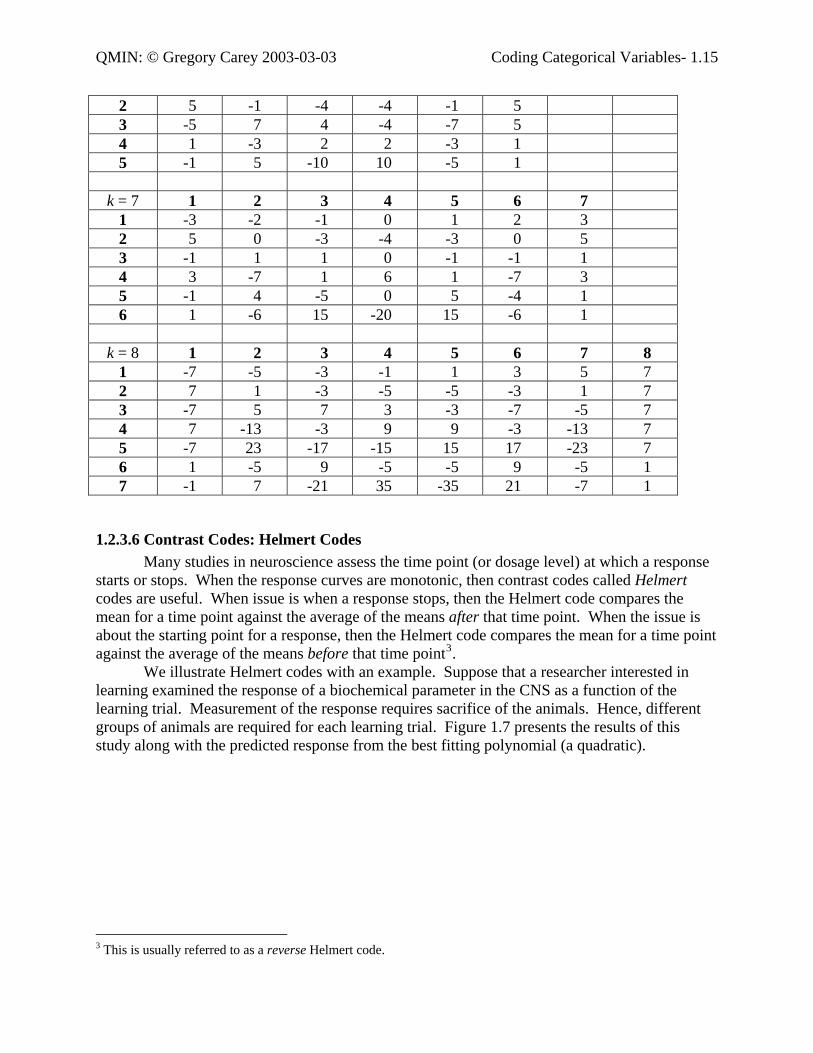
1.2.3.5 Contrast Codes: Orthogonal Polynomials When the levels of the ANOVA factor are ordered groups, then orthogonal polynomial contrast codes are often informative. The first code fits a linear term to the group means. That is, it fits a straight line through the means. The second code fits a quadratic term—i.e., a parabola. The third fits a cubic, the fourth, a quartic, and so on. The key assumption is that the groups are evenly spaced. The use of orthogonal polynomial contrast codes is very similar to the use of regression with ordered groups discussed in Section X.X. Regression with ordered groups, moreover, is much easier to apply to data, especially when the statistical package does not have contrast options with an ANOVA, ANCOVA, or GLM procedure. Hence, the reader could use the techniques outlined in Section X.X to fit orthogonal polynomials. The major difference between contrast codes in ANOVA and polynomial regression with ordered group lies in the error term for the F ratio. With k levels to an ANOVA factor, the error variance from a onwway ANOVA may be viewed as the error from fitting a polynomial of order (k – 1) to the data. Hence, if there are five levels, then the error variance from a oneway ANOVA is equal to fitting four orthogonal contrast codes—linear, quadratic, cubic, and quartic. In regression with ordered groups, however, the error term is derived from the best fitting polynomial, which could be a quadratic. Still, the difference between ANOVA with orthogonal polynomial contrast codes and regression with ordered groups should be slight. The reason is that the higher order polynomials ignored in the regression are insignificant and hence will not greatly reduce error. Coding schemes for orthogonal polynomials for up to eight levels of an ANOVA factor are presented in Table 1.6. Note that is it not necessary to fit all terms to an ANOVA factor. For example, if the ANOVA factor has five levels, it is permissible to test only the linear and the quadratic term.

Table 1.6 Orthogonal polynomial codes for ANOVA factors with up to eight levels.

Order: Level of ANOVA factor:

k = 3 1 2 3 1 -1 0 1 2 -1 2 -1

k = 4 1 2 3 4 1 -3 -1 1 3 2 1 -1 -1 1 3 -1 3 -3 1

k = 5 1 2 3 4 5 1 -2 -1 0 1 2 2 2 -1 -2 -1 2 3 -1 2 0 -2 1 4 1 -4 6 -4 1

k = 6 1 2 3 4 5 6 1 -5 -3 -1 1 3 5


2 5 -1 -4 -4 -1 5 3 -5 7 4 -4 -7 5 4 1 -3 2 2 -3 1 5 -1 5 -10 10 -5 1

k = 7 1 2 3 4 5 6 7 1 -3 -2 -1 0 1 2 3 2 5 0 -3 -4 -3 0 5 3 -1 1 1 0 -1 -1 1 4 3 -7 1 6 1 -7 3 5 -1 4 -5 0 5 -4 1 6 1 -6 15 -20 15 -6 1

k = 8 1 2 3 4 5 6 7 8 1 -7 -5 -3 -1 1 3 5 7 2 7 1 -3 -5 -5 -3 1 7 3 -7 5 7 3 -3 -7 -5 7 4 7 -13 -3 9 9 -3 -13 7 5 -7 23 -17 -15 15 17 -23 7 6 1 -5 9 -5 -5 9 -5 1 7 -1 7 -21 35 -35 21 -7 1

1.2.3.6 Contrast Codes: Helmert Codes Many studies in neuroscience assess the time point (or dosage level) at which a response starts or stops. When the response curves are monotonic, then contrast codes called Helmert codes are useful. When issue is when a response stops, then the Helmert code compares the mean for a time point against the average of the means after that time point. When the issue is about the starting point for a response, then the Helmert code compares the mean for a time point against the average of the means before that time point3. We illustrate Helmert codes with an example. Suppose that a researcher interested in learning examined the response of a biochemical parameter in the CNS as a function of the learning trial. Measurement of the response requires sacrifice of the animals. Hence, different groups of animals are required for each learning trial. Figure 1.7 presents the results of this study along with the predicted response from the best fitting polynomial (a quadratic).

3 This is usually referred to as a reverse Helmert code.


Figure 1.7 Mean (+/- 1 SEM) responses for learning trials along with the predicted values from the best fitting polynomial.

It is obvious from both the plot of observed means and the quadratic that the response increases until the fourth trial. Let us see whether the Helmert codes reveal that. The ANOVA factor in this example can be called Trial Number with levels of Trial1 through Trial6. Because there are 6 levels, we construct 5 contrast-coded variables. The first of these compares the mean of Trial 1 against the average of the means of Trials 2 through 6. This code is completely analogous to testing a “Control” (here, Trial1) against the average of “Treatments” (here, Trials 2 through 6). Hence, the equation for this variable is 05 654321 =−−−−− YYYYYY . The second Helmert code is designed to test whether the mean for the next level of the ANOVA factor, Trial2, differs from the overall mean of the remaining trials, 3 through 6. Here, we assign a value of 0 to Trial 1 because we are not interested in that any more, treat Trial2 as a “Control” and the remaining trials as “Treatments.” The resulting code is 040 654321 =−−−−+ YYYYYY . These and the remaining contrast codes are given in Table 1.7. Note that all rows in Table 1.7 sum to 0, a necessity for contrast codes. Note also that Helmert codes are orthogonal.


The product of the codes in each of the first four columns of Table 1.7 is 0. The product of the 5th column is 1, while the product of the last column is -1. Hence, the sum of the products equals 1 – 1 = 0. This is true of all Helmert codes, regardless of the number of levels.

Table 1.7 Example of reverse Helmert codes used to detect the ending point of a response.

Value assigned to level: Contrast-coded

Variable: Trial1

Trial2

Trial3

Trial4

Trial5

Trial6

Trial1 vs Rest 5 -1 -1 -1 -1 -1 Trial2 vs Rest 0 4 -1 -1 -1 -1 Trial3 vs Rest 0 0 3 -1 -1 -1 Trial4 vs Rest 0 0 0 2 -1 -1 Trial5 vs Rest 0 0 0 0 1 -1

We now use the Helmert contrast-coded variables as the independent variables in the GLM. Fitting these to the data from Figure 1.7 gives a significant overall fit—R2 = .39, df = (5, 84), p < .0001. Hence, we can interpret the significance of the individual contrast-coded variables with some confidence. Figure 1.8 gives those results. We see that the results of Trial1 vs Rest through Trial3 vs Rest are significant. The remaining two variables are not significant. Hence, we conclude—as Figure 1.7 clearly illustrates—that the response stops changing at Trial4.

Figure 1.8 Results of testing Helmert contrast-coded variables.

Contrast DF Contrast SS Mean Square F Value Pr > F Trial1 vs Rest 1 668.3168000 668.3168000 39.71 <.0001 Trial2 vs Rest 1 115.1960333 115.1960333 6.84 0.0105 Trial3 vs Rest 1 77.7493889 77.7493889 4.62 0.0345 Trial4 vs Rest 1 1.9067778 1.9067778 0.11 0.7373 Trial5 vs Rest 1 40.1363333 40.1363333 2.38 0.1263

The process of ascertaining the starting point for a response works in the opposite way. Here, the type of relationship starts out “flat” and then rapidly ascends (or descends). Figure 1.9 illustrates such a curve. The Helmert codes for detecting the starting Trial for the response (which is Trial 5) are given in Table 1.8.


Figure 1.9 Mean (+/- 1 SEM) responses for learning trials along with the predicted values from the best fitting polynomial; example of Helmert contrast coding to determine the starting point of a response.

Table 1.8 Example of reverse Helmert codes to detect the starting point of a response.

Value assigned to level: Contrast-coded

Variable: Trial1

Trial2

Trial3

Trial4

Trial5

Trial6

Rest vs Trial 2 -1 1 0 0 0 0 Rest vs Trial 3 -1 -1 2 0 0 0 Rest vs Trial 4 -1 -1 -1 3 0 0 Rest vs Trial 5 -1 -1 -1 -1 4 0 Rest vs Trial 6 -1 -1 -1 - 1 -1 5

1.2.3.7 Implementing contrast codes: GLM Procedures with “Contrast” statements Most modern statistical packages have the equivalent of a “Contrast” statement that allows one to provide contrast codes within an ANOVA, ANCOVA, or GLM procedure. In


these situations, the procedure will perform the classic ANOVA and then provide statistical tests for the hypotheses generated by the contrast code. Figure 1.10 gives the SAS Code and the output from PROC GLM in SAS used to analyze the PKC-gamma data.4 The code that generated this output contained two contrast statements, both designed to explore the effect of knocking out a PKC-gamma allele. The first contrast statement assigned the numeric values of 2, -1, and -1 to, respectively, genotypes ++, +-, and --. This contrast asks whether the average of the two genotypes having at least one knockout allele differs from the wild-type genotype. The second contrast assigned codes of 0, -1, and 1; this tests whether the heterozygote mean differs from the homozygote knockout mean.

Figure 1.10 SAS Code and Output from a Oneway ANOVA with Orthogonal Contrasts.

SAS Code: PROC GLM DATA=glmlib.pkcgamma; CLASS Genotype; MODEL Open_Arm = Genotype; CONTRAST '++ v Rest' Genotype 2 -1 -1 / E; CONTRAST '+- v --' Genotype 0 1 -1 / E; RUN; SAS Output: Dependent Variable: Open_Arm Percent time in open arm Sum of Source DF Squares Mean Square F Value Pr > F Model 2 1154.920444 577.460222 10.91 0.0002 Error 42 2223.837333 52.948508 Corrected Total 44 3378.757778 R-Square Coeff Var Root MSE Open_Arm Mean 0.341818 59.53559 7.276573 12.22222 Source DF Type III SS Mean Square F Value Pr > F Genotype 2 1154.920444 577.460222 10.91 0.0002 Contrast DF Contrast SS Mean Square F Value Pr > F ++ v Rest 1 291.960111 291.9601111 5.51 0.0236 +- v -- 1 862.960333 862.9603333 16.30 0.0002

4 The E option to the contrast statement prints out the levels of genotype (++. +-. and --) and the numeric contrast codes. This is always a recommended procedure to assure that the correct numbers are being assigned to the levels of the ANOVA factor.


The initial part of the output is identical to that of a oneway ANOVA with Genotype as the ANOVA factor. The only difference is the last section of output that gives the results of the two contrasts. The routine computes the SS for a contrast and the MS for the contrast. (Because a contrast always involves 1 degree of freedom, the MS for the contrast will always equal the SS). The F ratio for the contrast equals the MS for that contrast divided by the error MS from the model. Hence, the F ratio for the first contrast (“++ v Rest”) will equal

51.59485.529601.291

Rest v ==++F .

The numerator degrees of freedom for this F equal the df for the contrast (i.e., 1), and the denominator df equals the error df for the model (i.e., 42). Hence, the p value is the probability of observing an F greater than 5.51 from an F distribution with (1, 42) degrees of freedom. Because the observed p value of .02 is less than .05, we reject the null hypothesis that the knockout of at least one PKC-gamma allele has no effect on the percent of time spent in the open arm of an elevated plus-maze. The F for the second contrast (“+- v --“) divides the MS for this contrast by the error MS:

30.169485.529603.862

-- v ==−+F .

The df for this contrast will also be (1, 42). Because the p value for this test is much less than .05, we conclude that the mean for the heterozygote is significantly different from that of the double knockout homozygote. Note that these contrast codes are orthogonal and the ANOVA design is balanced (15 mice per genotype). Hence, the SS for both contrasts in Figure 1.10 add up to the SS for the ANOVA factor Genotype. Figure 1.11 presents results from fitting two non-orthogonal contrasts to the PKC-gamma data. The first contrast assigned the codes 1, -1, and 0 to, respectively genotypes ++, +-, and --, thus testing the difference between the means of the wild-type homozygote and the heterozygote. The second contrast used the codes of 1, 0 and -1, so it tests for mean differences between the wild-type homozygote and the double knockout homozygote.


Figure 1.11 Output from a oneway ANOVA with non-orthogonal contrasts.

SAS Code: PROC GLM DATA=glmlib.pkcgamma; CLASS Genotype; MODEL Open_Arm = Genotype; '++ v +-' Genotype 1 -1 0 / E; CONTRAST '++ v --' Genotype 1 0 -1 / E; CONTRAST RUN;

Dependent Variable: Open_Arm Percent time in open arm Sum of Source DF Squares Mean Square F Value Pr > F Model 2 1154.920444 577.460222 10.91 0.0002 Error 42 2223.837333 52.948508 Corrected Total 44 3378.757778 R-Square Coeff Var Root MSE Open_Arm Mean 0.341818 59.53559 7.276573 12.22222 Source DF Type III SS Mean Square F Value Pr > F Genotype 2 1154.920444 577.460222 10.91 0.0002 Contrast DF Contrast SS Mean Square F Value Pr > F ++ v +- 1 0.0120000 0.0120000 0.00 .9881 ++ v -- 1 869.4083333 869.4083333 16.42 .0002

SAS Output:

Just as in the orthogonal contrast, the F statistic for a non-orthogonal contrast equals the MS for that contrast divided by the error MS for the model, and the df for the contrast has 1 in the numerator and the error degrees of freedom in the denominator. The first contrast (“++ v +-“) is not significant. This agrees well with the observed data in Figure X.X (see Section X.X) which reveals only a small mean difference between the ++ and the +- genotypes. The second contrast (“++ v --“) is highly significant, consistent with the large mean difference between the ++ and the – genotypes in Figure X.X. There is one, very critical piece of advice for using “contrast” or analogous statements in a software package—always check to make certain the correct codes are being assigned to the correct groups. Statistical packages can differ in the way in which they order groups—e.g., alphabetic/numeric order versus the order in which they appear in the data set. If is always incumbent on the researcher to examine the output to make certain that the appropriate contrast is being implemented by the software.


1.2.3.8 Implementing contrast codes: Software without “Contrast” statements Some statistical software may not provide the option of “Contrast” statements with their ANOVA, ANCOVA, or GLM routines or the syntax of such statements is difficult to understand. One can still perform contrasts in these cases. Here, the secret is to create new variables for the contrasts, one variable for each contrast. If you create (k – 1) contrast variables and if the contrasts are orthogonal, then the results from the regression will be identical to those from the ANOVA with the contrast statement. For example, in the coding scheme used above in Figure 1.10, we would create a new variable—let us call it CC1—that has a value of 2 if the genotype is ++ and a value of -1 otherwise. The second new variable, CC2, would have a value of 0 for genotype ++, 1 for genotype +-, and -1 for genotype --. We would then regress the dependent variable on CC1 and CC2. Figure 1.12 gives the SAS code and the output from this regression.

Figure 1.12 Solving for contrast-coded variables using regression: orthogonal contrast codes.


SAS Code: DATA temp; SET glmlib.pkcgamma; IF Genotype='++' THEN CC1=2; ELSE CC1=-1; IF Genotype='++' THEN CC2=0; ELSE IF Genotype='+-' THEN CC2=1; ELSE CC2=-1; RUN; PROC REG DATA=temp; MODEL Open_Arm = CC1 CC2; RUN;

Dependent Variable: Open_Arm Percent time in open arm Analysis of Variance Sum of Mean Source DF Squares Square F Value Pr > F Model 2 1154.92044 577.46022 10.91 0.0002 Error 42 2223.83733 52.94851 Corrected Total 44 3378.75778 Root MSE 7.27657 R-Square 0.3418 Dependent Mean 12.22222 Adj R-Sq 0.3105 Coeff Var 59.53559 Parameter Standard Variable Label DF Estimate Error t Value Pr > |t| Intercept Intercept 1 12.22222 1.08473 11.27 <.0001 CC1 ++ v Rest 1 -1.80111 0.76702 -2.35 0.0236 CC2 +- v -- 1 -5.36333 1.32851 -4.04 0.0002

SAS Output:

Note that the analysis of variance table in Figure 1.12 is identical to the one in Figure 1.10. Results of the two contrast-coded variables, CC1 and CC2, are also identical to the two contrasts in Figure 1.10 albeit expressed in a different form. The F statistics in Figure 1.10 are the square of the t statistics in Figure 1.12. The p values for the contrast-coded variables in Figure 1.12 are identical to those for the Contrast statements used to generate the results in Figure 1.10. If (1) there are fewer than (k – 1) contrasts or (2) the contrasts are non-orthogonal, then the solution is still tractable, albeit more cumbersome. Follow these steps:

(1) Perform a classic ANOVA on the data. (2) Record the error df and the error MS from the results of the classic ANOVA.


(3) Compute new independent variables using the contrast codes. (4) Using a regression procedure, regress the dependent variable on the first contrast-coded

(5)

(6) istic will have a numerator degrees of freedom equal to 1; the denominator df

(7) hat, because every contrast will have

)

(8) these steps

e illustrate this procedure using the non-orthogonal contrast codes for the PKC-gamma

igure 1.13 Regression analysis for non-orthogonal contrasts: first independent variable.

e

independent variable; do not regress it on all the contrast-coded independent variables. Take the model sum of squares from this regression and divide it by the error MS from the classic ANOVA; this gives the F statistic for this contrast-coded independent variable. The F statwill equal the error df from the classic ANOVA. Compute (or look up) the p value for the F; note tthe same degrees of freedom in the numerator and in the denominator, the critical valuefor the F will be the same for all contrasts; hence, you may prefer to compute (or look upthe critical value for F and compare the observed F to that critical value. Repeat steps (4) through (7) for the next contrast-coded variable; continueuntil all contrast-coded variables have been analyzed. W

data given above in Figure 1.11. Instead of reproducing the classic ANOVA, we can take the relevant numbers from that Figure—i.e., error df = 42 and error MS = 52.9485.

F

The first step is to construct a new independent variable from the first contrast code. This

Dependent Variable: Open_Arm Percent time in open arm Analysis of Variance Sum of Mean Source DF Squares Square F Value Pr > F Model 1 0.01200 0.01200 0.00 0.9902 Error 43 3378.74578 78.57548 Corrected Total 44 378.75778 Root MSE 8.86428 R-Square 0.0000 Dependent Mean 12.22222 Adj R-Sq -0.0233 Coeff Var 72.52594 Parameter Standard Variable Label DF Estimate Error t Value Pr > |t| Intercept Intercept 1 12.22222 1.32141 9.25 <.0001 CC1 ++ v +- 1 -0.02000 1.61839 -0.01 0.9902

new variable, which we shall call CC1, has a value of 1 if the genotype is ++, a value of -1 if the genotype is +-, or a value of 0 if the genotype is --. Next, we regress the dependent variable, Open_Arm, on independent variable CC1. The results from this regression are given in Figur1.13. The sum of squares for this regression is .012. (Note that this is also the value for the SS of the contrast using a contrast statement in Figure 1.11). Hence, the F ratio for this contrast is


002.09485.52

012.error

CC1CC1 ===

MSSSF .

The degrees of freedom for this F are (1, 42), and the p level is .988. Thus, there is no evidence that the means for the wild-type homozygote and the heterozygote differ. We now move to the second independent variable. This will have values of 1 (genotype ++), 0 (genotype +-), or -1 (genotype --). Calling this variable CC2, we regress dependent variable Open_Arm on CC2. The results are given in Figure 1.14.

Figure 1.14 Regression analysis for non-orthogonal contrasts: second independent variable.

Dependent Variable: Open_Arm Percent time in open arm Analysis of Variance Sum of Mean Source DF Squares Square F Value Pr > F Model 1 869.40833 869.40833 14.90 0.0004 Error 43 2509.34944 58.35696 Corrected Total 44 3378.75778 Root MSE 7.63917 R-Square 0.2573 Dependent Mean 12.22222 Adj R-Sq 0.2400 Coeff Var 62.50232 Parameter Standard Variable Label DF Estimate Error t Value Pr > |t| Intercept Intercept 1 12.22222 1.13878 10.73 <.0001 CC2 ++ v -- 1 -5.38333 1.39472 -3.86 0.0004

The SS for the model from this regression is 869.4083 (once again, the same number given in the Figure 1.11 using a contrast statement). Hence, the F statistic for the second contrast-coded independent variable is

42.169485.524083.869

error

2CC2 ===

MSSSF CC .

With df of (1, 42), the p level for this F is .0002. (You should verify that this F, its degrees of freedom, and the p value are the same as those in Figure 1.11). We conclude that there is strong evidence that the means for the two homozygotes differ. Note that we arrived at the same substantive results performing these hand calculations as we would have just examining the output from the two simple regressions in Figure 1.13 and Figure 1.14. This happened largely because of the example that we used. For the PKC-gamma data, the difference between the mean for genotype ++ and the mean for genotype +- is very small, so it is highly unlikely that a minor change in technique would ever make this difference significant. Similarly, the difference between the ++ mean and the – mean is very large; it would be very surprising if any reasonable test for this difference would not reach statistical significance. In general, however, the results from the simple regressions and those from the hand-calculated contrasts will not always be equal.


1.3 Examples:

1.3.1 Coding Several Hypotheses Sometimes a study involves several groups, but only a few comparisons are of interest. Suppose that a lab interested in developmental effects on anxiety administered a GABA blocker to rat pups for two weeks shortly after birth and then tested them as adults. Naturally, there would be a control group who received vehicle injections. In the adult testing, those rats who had received the GABA blocker are randomly divided into four groups: a control, and three groups, each administered an anxiolytic compound shortly before testing. The dependent variable in this case is a measure of startle. The group has two major hypotheses: (1) administration of the GABA antagonist in early postnatal weeks will result in increased anxiety as adults; and (2) this effect will be blocked by each of the three anxiolytic agents. Figure 1.15 presents the results of this hypothetical study.

Figure 1.15 Mean (+/1 SEM) startle as a function of early exposure to a GABA blocker and three anxiolytic drugs.


An overall ANOVA on these data would be inefficient because there are only two hypotheses to be tested. Hence, one can construct two sets of contrast codes, one for each hypothesis, and then examine the significance level of these two contrasts. Let CY denote the mean of the controls and 0Y through 3Y denote the means of the groups administered the GABA blocker, the subscript denoting the number of the anxiolytic drug. The very first contrast code would have the set of numbers (1 -1 0 0 0) for, respectively, the groups as ordered in Figure 1.15. This code embodies the following null hypothesis 0)(0)(0)(0)(1 0C3210C =−=+++− YYYYYYY . Substantively, this code tests whether the GABA antagonist had an effect on startle. The second code tests whether the three groups given the anxiolytic differ from the group previously administered the GABA blocker but receiving no anxiolytic before testing. The appropriate code here would be (0 3 -1 -1 -1), giving the null hypothesis

03

)(1)(1)(1)(3)(0 32103210C =

++−=−−−+

YYYYYYYYY .

Hence, this tests whether the GABA-inhibitor only group differs from the average mean of the GABA-inhibitors receiving an anxiolytic. Figure 1.16 presents the SAS code and the results of fitting the ANOVA to these data. Note that the groups were assigned numbers according to their order in Figure 1.15 (1 = Control, 2 = GABA blocker only, 3 = GABA blocker + Anxiolytic 1, etc.). Hence the order of the codes in the Contrast statement must reflect this order. Note that the overall ANOVA is not significant. This is not a problem because the two hypotheses are embodied in the contrasts. The only utility of the overall ANOVA is to give an estimate of the error variance that is used in testing the significant of the contrasts.


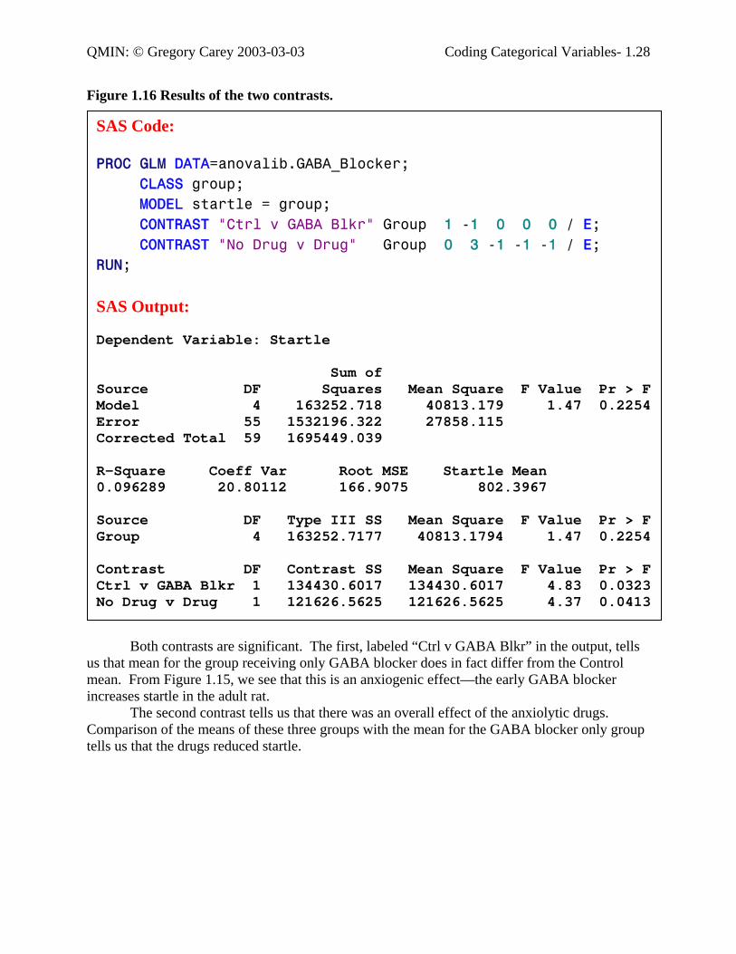
Figure 1.16 Results of the two contrasts.

SAS Code: PROC GLM DATA=anovalib.GABA_Blocker; CLASS group; MODEL startle = group; CONTRAST "Ctrl v GABA Blkr" Group 1 -1 0 0 0 / E; CONTRAST "No Drug v Drug" Group 0 3 -1 -1 -1 / E; RUN; SAS Output: Dependent Variable: Startle Sum of Source DF Squares Mean Square F Value Pr > F Model 4 163252.718 40813.179 1.47 0.2254 Error 55 1532196.322 27858.115 Corrected Total 59 1695449.039 R-Square Coeff Var Root MSE Startle Mean 0.096289 20.80112 166.9075 802.3967 Source DF Type III SS Mean Square F Value Pr > F Group 4 163252.7177 40813.1794 1.47 0.2254 Contrast DF Contrast SS Mean Square F Value Pr > F Ctrl v GABA Blkr 1 134430.6017 134430.6017 4.83 0.0323 No Drug v Drug 1 121626.5625 121626.5625 4.37 0.0413

Both contrasts are significant. The first, labeled “Ctrl v GABA Blkr” in the output, tells us that mean for the group receiving only GABA blocker does in fact differ from the Control mean. From Figure 1.15, we see that this is an anxiogenic effect—the early GABA blocker increases startle in the adult rat. The second contrast tells us that there was an overall effect of the anxiolytic drugs. Comparison of the means of these three groups with the mean for the GABA blocker only group tells us that the drugs reduced startle.


1.4 References Cohen, J. & Cohen, P. (1983). Applied Multiple Regression/Correlation Analysis for the Behavioral Sciences, 2nd Ed. Hillsdale, NJ: Lawrence Erlbaum. Judd, C.M. & McClelland, G.H. (1989). Data Analysis: A Model-Comparison Approach. New York: Harcourt, Brace, Jovanovich. Falconer, D.S. & Mackay, T.F.C. (1996). Introduction to Quantitative Genetics, 4th Ed. New York: Prentice Hall.


1.5 Tables Table 1.1 Example of Coding according to a Mathematical Model ............................................ 1.7 Table 1.2 Descriptive statistics for the PKC-gamma data set...................................................... 1.9 Table 1.3 Example contrast codes for the three levels of PKC-gamma genotype..................... 1.10 Table 1.4 Examples of orthogonal and non-orthogonal contrast coded variables. .................... 1.12 Table 1.5 Non-orthogonal contrast codes for comparing each treatment mean to a control mean.

............................................................................................................................................ 1.13 Table 1.6 Orthogonal polynomial codes for ANOVA factors with up to eight levels. ............. 1.14 Table 1.7 Example of reverse Helmert codes used to detect the ending point of a response. ... 1.17 Table 1.8 Example of reverse Helmert codes to detect the starting point of a response. .......... 1.18


Figures Figure 1.1 Mean (+/- 1 SEM) cell death index for as a function of type of drug and dose of

BDNF................................................................................................................................... 1.2 Figure 1.2 Classic ANOVA results on BDNF data set................................................................ 1.3 Figure 1.3 GLM results using contrast codes on the BDNF data set........................................... 1.3 Figure 1.4 GLM results using contrast codes and a quantitative variable for dose of BDNF. .... 1.5 Figure 1.5 Advantages and Disadvantages of Coding ANOVA Factors,.................................... 1.6 Figure 1.6 A model for the analysis of a quantitative phenotype for a genetic locus with two

alleles, A1 and A2................................................................................................................ 1.7 Figure 1.7 Mean (+/- 1 SEM) responses for learning trials along with the predicted values from

the best fitting polynomial. ................................................................................................ 1.16 Figure 1.8 Results of testing Helmert contrast-coded variables. ............................................... 1.17 Figure 1.9 Mean (+/- 1 SEM) responses for learning trials along with the predicted values from

the best fitting polynomial; example of Helmert contrast coding to determine the starting point of a response. ............................................................................................................ 1.18

Figure 1.10 SAS Code and Output from a Oneway ANOVA with Orthogonal Contrasts........ 1.19 Figure 1.11 Output from a oneway ANOVA with non-orthogonal contrasts............................ 1.21 Figure 1.12 Solving for contrast-coded variables using regression: orthogonal contrast codes.1.22 Figure 1.13 Regression analysis for non-orthogonal contrasts: first independent variable....... 1.24 Figure 1.14 Regression analysis for non-orthogonal contrasts: second independent variable. . 1.25 Figure 1.15 Mean (+/1 SEM) startle as a function of early exposure to a GABA blocker and three

anxiolytic drugs.................................................................................................................. 1.26 Figure 1.16 Results of the two contrasts.................................................................................... 1.28

Documents

1 Coding Categorical Variables - University of Colorado ...psych.colorado.edu/~carey/Courses/PSYC5741/handouts/Coding...1 Coding Categorical Variables ... The error bars, however,