Embed Size (px)
Citation preview

1
Clustering
Instructor: Qiang YangHong Kong University of Science and Technology
Thanks: J.W. Han, I. Witten, E. Frank

2
Essentials
Terminology: Objects = rows = records Variables = attributes = features
A good clustering method high on intra-class similarity and low on inter-class similarity
What is similarity? Based on computation of distance
Between two numerical attributes Between two nominal attributes Mixed attributes

3
The database
npn
ipi
p
xx
xx
xx
1
1
111
......
...
...
...
...
......
Object i

4
Numerical Attributes
Distances are normally used to measure the similarity or dissimilarity between two data objects
Euclideandistance:
where i = (xi1, xi2, …, xip) and j = (xj1, xj2, …, xjp)
are two p-dimensional records, Manhattan distance
)||...||2|(|),( 22
2211 pp jx
ix
jx
ix
jx
ixjid
||...||||),(2211 pp jxixjxixjxixjid

5
Binary Variables ({0, 1}, or {true, false})
A contingency table for binary data
Simple matching coefficient
Invariant of coding of binary variable: if you assign 1 to “pass” and
0 to “fail”, or the other way around, you’ll get the same distance
value.
dcbacb jid
),(
pdbcasum
dcdc
baba
sum
0
1
01
Row i
Row j

6
Nominal Attributes
A generalization of the binary variable in that it can take more than 2 states, e.g., red, yellow, blue, green
Method 1: Simple matching m: # of matches, p: total # of variables
Method 2: use a large number of binary variables creating a new binary variable for each of the M
nominal states
pmpjid ),(

7
Other measures of cluster distance
Minimum distance
Max distance
Mean distance
Avarage distance
|'|min),( ', PPCCd CjpCipji
|'|max),( ', PPCCd CjpCipji
jiji mmCCd ),(
CjpCip
PPnn
CCdji
ji |'|1
),(

8
Major clustering methods
Partition based (K-means) Produces sphere-like clusters Good when
know number of clusters, Small and med sized databases
Hierarchical methods (Agglomerative or divisive) Produces trees of clusters Fast
Density based (DBScan) Produces arbitrary shaped clusters Good when dealing with spatial clusters (maps)
Grid-based Produces clusters based on grids Fast for large, multidimensional databases
Model-based Based on statistical models Allow objects to belong to several clusters

9
The K-Means Clustering Method: for numerical attributes
Given k, the k-means algorithm is implemented in four steps: Partition objects into k non-empty subsets Compute seed points as the centroids of the
clusters of the current partition (the centroid is the center, i.e., mean point, of the cluster)
Assign each object to the cluster with the nearest seed point
Go back to Step 2, stop when no more new assignment

10
The mean point
0
0.5
1
1.5
2
2.5
3
3.5
4
4.5
0 1 2 3 4 5
X
X Y
1 2
2 4
3 3
4 2
2.5 2.75
The mean point can be a virtual point

11
The K-Means Clustering Method
Example
0
1
2
3
4
5
6
7
8
9
10
0 1 2 3 4 5 6 7 8 9 100
1
2
3
4
5
6
7
8
9
10
0 1 2 3 4 5 6 7 8 9 10
0
1
2
3
4
5
6
7
8
9
10
0 1 2 3 4 5 6 7 8 9 10
0
1
2
3
4
5
6
7
8
9
10
0 1 2 3 4 5 6 7 8 9 10
0
1
2
3
4
5
6
7
8
9
10
0 1 2 3 4 5 6 7 8 9 10
K=2
Arbitrarily choose K object as initial cluster center
Assign each objects to most similar center
Update the cluster means
Update the cluster means
reassignreassign

12
Comments on the K-Means Method
Strength: Relatively efficient: O(tkn), where n is # objects, k is # clusters, and t is # iterations. Normally, k, t << n.
Comment: Often terminates at a local optimum. Weakness
Applicable only when mean is defined, then what about categorical data?
Need to specify k, the number of clusters, in advance Unable to handle noisy data and outliers too well Not suitable to discover clusters with non-convex
shapes

13
Robustness
0
0.5
1
1.5
2
2.5
3
3.5
4
4.5
1 10 100 1000
X
X Y
1 2
2 4
3 3
400 2
101.5 2.75

14
Variations of the K-Means Method
A few variants of the k-means which differ in
Selection of the initial k means
Dissimilarity calculations
Strategies to calculate cluster means
Handling categorical data: k-modes (Huang’98)
Replacing means of clusters with modes
Using new dissimilarity measures to deal with categorical objects
Using a frequency-based method to update modes of clusters
A mixture of categorical and numerical data: k-prototype method

15
K-Modes: See J. X. Huang’s paper online (Data Mining and Knowledge Discovery Journal, Springer)

16
Formalization of K-Means

17
K-Means: Cont.

18
K-Modes: See J. X. Huang’s paper online (Data Mining and Knowledge Discovery Journal, Springer)

19
K-Modes (Cont.)

20
K-Modes

21
K-Modes: Cost Function

22
Finding K-Modes

23
Mixed Types: K-Prototypes

24
K-Modes: Evaluation Data

25
K-Modes: Evaluation

26
Some Experiments

27
What is the problem of k-Means Method?
The k-means algorithm is sensitive to outliers !
Since an object with an extremely large value may
substantially distort the distribution of the data.
K-Medoids: Instead of taking the mean value of the object in
a cluster as a reference point, medoids can be used, which is
the most centrally located object in a cluster.
0
1
2
3
4
5
6
7
8
9
10
0 1 2 3 4 5 6 7 8 9 100
1
2
3
4
5
6
7
8
9
10
0 1 2 3 4 5 6 7 8 9 10

28
The K-Medoids Clustering Method
Find representative objects, called
medoids, in clusters
Medoids are located in the center of the
clusters.
Given data points, how to find the
medoid?
0
1
2
3
4
5
6
7
8
9
10
0 1 2 3 4 5 6 7 8 9 10

29
K-Medoids: most centrally located objects

30
CLARA

31
CLASA: Simulated Annealing

32
Sampling based method: MCMRS

33
KMedoids: Evaluation

34
Density-Based Clustering Methods
Clustering based on density (local cluster criterion), such as density-connected points
Major features: Discover clusters of arbitrary shape Handle noise One scan Need density parameters as termination
condition Several interesting studies:
DBSCAN: Ester, et al. (KDD’96) OPTICS: Ankerst, et al (SIGMOD’99). DENCLUE: Hinneburg & D. Keim (KDD’98) CLIQUE: Agrawal, et al. (SIGMOD’98)

35
Density-Based Clustering
Clustering based on density (local cluster criterion), such as density-connected points
Each cluster has a considerable higher density of points than outside of the cluster

36
Density-Based Clustering: Background
Two parameters: : Maximum radius of the neighbourhood MinPts: Minimum number of points in an Eps-
neighbourhood of that point
N(p): {q belongs to D | dist(p,q) <= } Directly density-reachable: A point p is directly
density-reachable from a point q wrt. , MinPts if
1) p belongs to N(q)
2) core point condition:
|N (q)| >= MinPts
pq
MinPts = 5
= 1 cm

37
Density-Based Clustering: Background (II)
Density-reachable: A point p is density-reachable
from a point q wrt. , MinPts if there is a chain of points p1, …, pn, p1 = q, pn = p such that pi+1 is directly density-reachable from pi
Density-connected A point p is density-connected to
a point q wrt. , MinPts if there is a point o such that both, p and q are density-reachable from o wrt. and MinPts.
p
qp1
p q
o

38
DBSCAN: Density Based Spatial Clustering of Applications with Noise
Relies on a density-based notion of cluster: A cluster is defined as a maximal set of density-connected points
Discovers clusters of arbitrary shape in spatial databases with noise
Core
Border
Outlier
Eps = 1cm
MinPts = 5

39
DBSCAN: The Algorithm
Arbitrary select a point p
Retrieve all points density-reachable from p wrt and MinPts.
If p is a core point, a cluster is formed.
If p is a border point, no points are density-reachable from p and DBSCAN visits the next point of the database.
Continue the process until all of the points have been processed.

40
DBSCAN Properties
Generally takes O(nlogn) time
Still requires user to supply Minpts and
Advantage Can find points of
arbitrary shape Requires only a minimal
(2) of the parameters
41
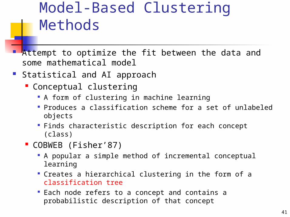
Model-Based Clustering Methods
Attempt to optimize the fit between the data and some mathematical model
Statistical and AI approach Conceptual clustering
A form of clustering in machine learning Produces a classification scheme for a set of unlabeled
objects Finds characteristic description for each concept (class)
COBWEB (Fisher’87) A popular a simple method of incremental conceptual
learning Creates a hierarchical clustering in the form of a
classification tree Each node refers to a concept and contains a probabilistic
description of that concept

42
The COBWEB Conceptual Clustering Algorithm 8.8.1
The COBWEB algorithm was developed by D. Fisher in the 1990 for clustering objects in a object-attribute data set.
Fisher, Douglas H. (1987) Knowledge Acquisition Via Incremental Conceptual Clustering
The COBWEB algorithm yields a classification tree that characterizes each cluster with a probabilistic description
Probabilistic description of a node: (fish, prob=0.92) Properties:
incremental clustering algorithm, based on probabilistic categorization trees
The search for a good clustering is guided by a quality measure for partitions of data
COBWEB only supports nominal attributes CLASSIT is the version which works with nominal and numerical attributes

43
The Classification Tree Generated by the COBWEB Algorithm

44
Input: A set of data like before
Can automatically guess the class attribute
That is, after clustering, each cluster more or less corresponds to one of Play=Yes/No category
Example: applied to vote data set, can guess correctly the party of a senator based on the past 14 votes!

45
Clustering: COBWEB
• In the beginning tree consists of empty node
• Instances are added one by one, and the tree is updated appropriately at each stage
• Updating involves finding the right leaf an instance (possibly restructuring the tree)
• Updating decisions are based on partition utility and category utility measures

46
Clustering: COBWEB
class
pair value-attribute
kC
ijViA
)|( kCijViAP
:similarity class-Intra
The larger this probability, the greater the proportion of class members sharing the value (Vij) and the more predictable the value is of class members.

47
Clustering: COBWEB
)|( ijViAkCP
:similarity class-Inter
The larger this probability, the fewer the objects that share this value (Vij) and the more predictive the value is of class Ck.

48
Clustering: COBWEB
)|(*)|(*)(),...,,(1
21 kiji
n
k i jijikijin CVAPVACPVAPCCCPU
:Utility Partition
The formula is a trade-off between intra-class similarity and inter-class dissimilarity, summed across all classes (k), attributes (i), and values (j).

49
Clustering: COBWEB
n
k i jkijikn
kijik
ijik
iji
ijik
ijiijikiji
CVAPCPCCCPU
CVAPCP
VACP
VAP
VACPVAPVACPVAP
1
221
)|()(),...,,(
)|(*)(
),(
)(
),(*)()|(*)(
:as rewritten be can Utility Partition
:rule Bayes' using equation the Rewrite

50
Clustering: COBWEB
n
k i jijikijikn
VAPCVAPCPCCCCU1
2221
)()|()(),...,,(
:Utility Category
Increase in the expected number of attribute values that can be correctly guessed (Posterior Probability)
The expected number of correct guesses give no such knowledge (Prior Probability)

51
The Category Utility Function
The COBWEB algorithm operates based on the so-called category utility function (CU) that measures clustering quality.
If we partition a set of objects into m clusters, then the CU of this particular partition is
m
VAPCVAPCPi j
ijii j
kiji
m
kk
22
1
|
Question: Why divide bym?- hint: if m=#objects, CU is max!

52
Insights of the CU Function
For a given object in cluster Ck, if we guess its attribute values according to the probabilities of occurring, then the expected number of attribute values that we can correctly guess is
i jkiji CVAP 2|

53
Given an object without knowing the cluster that the object is in, if we guess its attribute values according to the probabilities of occurring, then the expected number of attribute values that we can correctly guess is
i j
iji VAP 2

54
P(Ck)is incorporated in the CU function to give proper weighting to each cluster.
Finally, m is placed in the denominator to prevent over-fitting.

55
Question about CU
Are their other ways to define category utility for a partition?
For example, using information theory? Recall that mutual information I(X,Y) defines the
reduction of uncertainty in X when knowing Y: I(X,Y)=H(X)-H(X|Y), where H(X)=-p(X)log(X), and H(X|Y)=E[-p(X|Y)logp(X|Y)] over Y=y_i
Now, let X: X_i=(A_i=V_{ij}), Y: y_l=C_l I(A_i,C)=E_{clusters}(H(A_i)-H(A_i|C_j)} I(C)=E_{A_i}(H(A_i, C))

56
Finite mixtures
Probabilistic clustering algorithms model the data using a mixture of distributions
Each cluster is represented by one distribution The distribution governs the probabilities of
attributes values in the corresponding cluster They are called finite mixtures because there is
only a finite number of clusters being represented
Usually individual distributions are normal distribution
Distributions are combined using cluster weights

57
A two-class mixture modelA 51A 43B 62B 64A 45A 42A 46A 45A 45
B 62A 47A 52B 64A 51B 65A 48A 49A 46
B 64A 51A 52B 62A 49A 48B 62A 43A 40
A 48B 64A 51B 63A 43B 65B 66B 65A 46
A 39B 62B 64A 52B 63B 64A 48B 64A 48
A 51A 48B 64A 42A 48A 41
data
model
A=50, A =5, pA=0.6 B=65, B =2, pB=0.4

58
Using the mixture model
The probability of an instance x belonging to cluster A is:
with
The likelihood of an instance given the clusters is:
]Pr[),;(
]Pr[]Pr[]|Pr[
]|Pr[x
pxfx
AAxxA AAA
2
2
2
)(
21
),;(
x
exf
i
xx ]clusterPr[]cluster|Pr[]onsdistributi the|Pr[ ii

59
Learning the clusters
Assume we know that there are k clusters To learn the clusters we need to
determine their parameters I.e. their means and standard deviations
We actually have a performance criterion: the likelihood of the training data given the clusters
Fortunately, there exists an algorithm that finds a local maximum of the likelihood

60
The EM algorithm
EM algorithm: expectation-maximization algorithm Generalization of k-means to probabilistic
setting Similar iterative procedure:
1. Calculate cluster probability for each instance (expectation step)
2. Estimate distribution parameters based on the cluster probabilities (maximization step)
Cluster probabilities are stored as instance weights

61
More on EM
Estimating parameters from weighted instances:
Procedure stops when log-likelihood saturates
Log-likelihood (increases with each iteration; we wish it to be largest):
n
nnA www
xwxwxw
...
)(...)()(
21
2222
2112
n
nnA www
xwxwxw
......
21
2211
])|Pr[]|Pr[(log BxpAxp iBiAi