Embed Size (px)
Citation preview

1
Chapter 7
Filter Design Techniques (cont.)
2
Optimum Approximation Criterion (1)
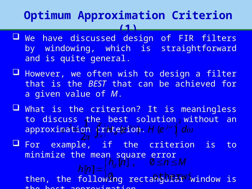
We have discussed design of FIR filters by windowing, which is straightforward and is quite general.
However, we often wish to design a filter that is the BEST that can be achieved for a given value of M.
What is the criterion? It is meaningless to discuss the best solution without an approximation criterion.
For example, if the criterion is to minimize the mean square error
then, the following rectangular window is the best approximation.
otherwise,0
0],[][
Mnnhnh d
deHeH jjd
22 )()(
2
1

3
Optimum Approximation Criterion (2)
However, the window methods generally have two problems:
Adverse behavior at discontinuities of H(ej); the error usually becomes smaller for frequencies away from the discontinuity (over-specified at those frequencies).
It does not permit individual control over approximation error in different bands (over-specified over some bands).
For many applications, better filters result from a minimax strategy (minimization of the maximum errors) or a frequency-weighted criterion.
Approximation error is spread out uniformly in frequency
Individual control of approximation error over different bands
Such criterion avoids the abovementioned over-specifications.
4
Optimum Approximation Criterion (3)
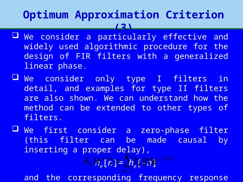
We consider a particularly effective and widely used algorithmic procedure for the design of FIR filters with a generalized linear phase.
We consider only type I filters in detail, and examples for type II filters are also shown. We can understand how the method can be extended to other types of filters.
We first consider a zero-phase filter (this filter can be made causal by inserting a proper delay),
he[n]= he[–n]
and the corresponding frequency response is ( L = M/2 is an integer)
njL
Lne
je enheA
][)(
5
Optimum Approximation Criterion (4)
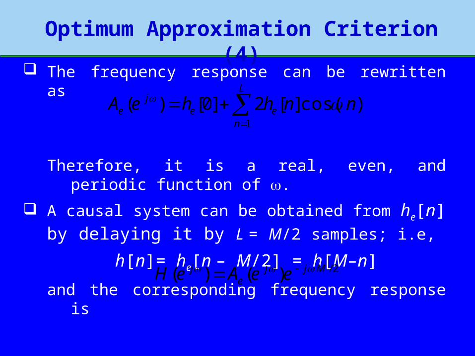
The frequency response can be rewritten as
Therefore, it is a real, even, and periodic function of .
A causal system can be obtained from he[n] by delaying it by L = M/2 samples; i.e,
h[n]= he[n – M/2] = h[M–n]
and the corresponding frequency response is
L
nee
je nnhheA
1
)cos(][2]0[)(
2/)()( Mjje
j eeAeH

6
Optimum Approximation Criterion (5)
A tolerance scheme for an approximation to a LPF with a real function Ae(ej).
Some of the parameters L, 1, 2, p, and s are fixed and an iterative procedure is used to obtain optimum adjustment of the remaining parameters.

7
Optimum Approximation Criterion (6)
There are several methods for FIR filter design. The Parks-McClellan algorithm (Remez algorithm) has become the dominant method for optimum design of FIR filters. This is because it is the most flexible and the most computationally efficient. We will discuss only that algorithm.
The Parks-McClellan algorithm is based on reformulating the filter design problem as a problem in polynomial approximation.
We note that the term cos(n) in Ae(ej) can be expressed as a
sum of powers of in the form
cos(n) =Tn(cos )
where Tn(x) = cos(ncos-1x) is the nth-order Chebyshev polynomial.

8
Chebyshev Polynomial
Chebyshev polynomial
Vn(x) is an nth polynomial of x.
)coshcosh()coscos()( 11 xNxNxVN
)()(2)(
,,12)(
,)(
,1)(
11
22
1
0
xVxxVxV
xxV
xxV
xV
NNN

9
Optimum Approximation Criterion (7)
Therefore, Ae(ej) can be expressed as an Lth-order
polynomial in cos namely
where
cos0
)()(cos)(
x
L
k
kk
je xPaeA
L
k
kk xaxP
0
)(
10
Optimum Approximation Criterion (8)
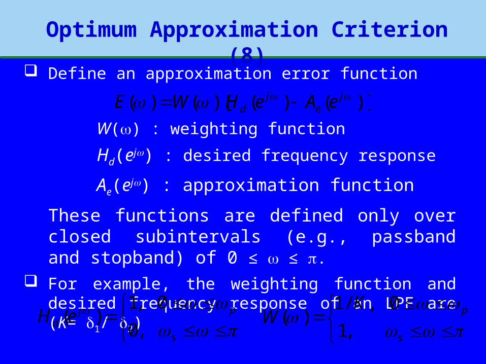
Define an approximation error function
W() : weighting function
Hd(ej) : desired frequency response
Ae(ej) : approximation function
These functions are defined only over closed subintervals (e.g., passband and stopband) of 0 ≤ ≤ .
For example, the weighting function and desired frequency response of an LPF are (K= 1/ 2)
)]()()[()( je
jd eAeHWE
s
pjd eH
,0
0,1)(
s
pKW
,1
0,/1)(

11
Optimum Approximation Criterion (9)
Note that, with weighting, the maximum weighted absolute approximation error is = 2 in both bands.
Typical frequency response.
Weighted error.
12
Optimum Approximation Criterion (10)
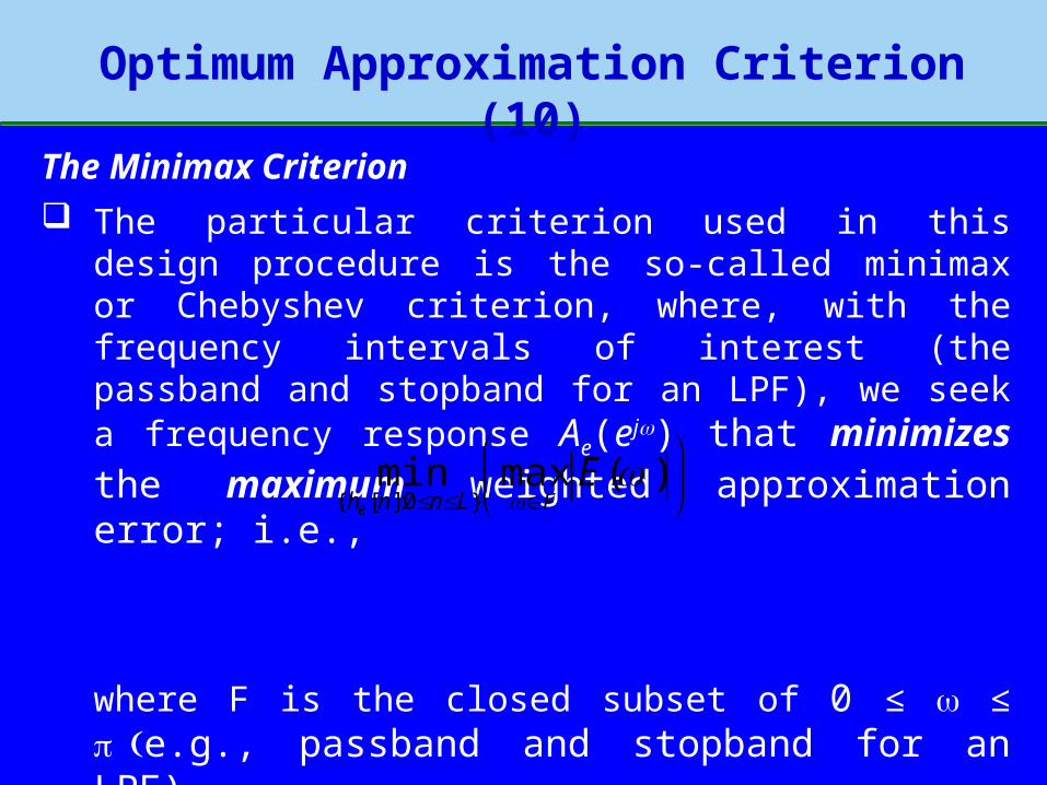
The Minimax Criterion
The particular criterion used in this design procedure is the so-called minimax or Chebyshev criterion, where, with the frequency intervals of interest (the passband and stopband for an LPF), we seek a frequency response Ae(ej) that minimizes the maximum weighted approximation error; i.e.,
where F is the closed subset of 0 ≤ ≤ e.g., passband and stopband for an LPF).
)(maxmin
}0:][{
E
FLnnhe
13
Optimum Approximation Criterion (11)
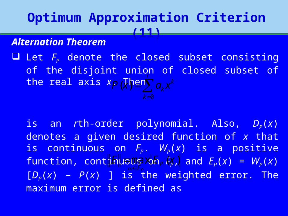
Alternation Theorem
Let FP denote the closed subset consisting of the disjoint union of closed subset of the real axis x. Then
is an rth-order polynomial. Also, DP(x) denotes a given desired function of x that is continuous on FP. WP(x) is a positive
function, continuous on FP, and EP(x) = WP(x)[DP(x) – P(x) ] is the weighted error. The maximum error is defined as
A necessary and sufficient condition that P(x) be the unique rth-order polynomial that minimizes ||E|| is that EP(x) exhibit at least (r+2) alternations.
)(max xEE PFP
r
k
kk xaxP
0
)(

14
Optimum Approximation Criterion (11)
(r +2) alternations means…
there must exist at least (r + 2) values xi in FP such that x1 < x2 <
…< xr+2 and such that EP(xi)= –EP(xi+1)=||E|| for i=1, 2,…, r +1.
Example … which one satisfies the alternation theorem (r =5)?

15
Optimal Type I Lowpass Filters (1)
For type I filters, the polynomial P(x) is the cosine polynomial Ae(ej) with the transformation of variable x=cos and r = L:
DP(x) and WP(x) become
and
respectively, and the weighted approximation error is
L
k
kkaP
0
)(cos)(cos
s
ppD
coscos1,0
1coscos,1)(cos
s
pp
KW
coscos1,0
1coscos,/1)(cos
)](cos)(cos)[(cos)(cos PDWE ppp

16
Optimal Type I Lowpass Filters (2)
Equivalent polynomial approximation function as a function of x=cos .

17
Optimal Type I Lowpass Filters (3)
Properties
The maximum possible number of alternations of the error is L+3.
An Lth-degree polynomial can have at most (L–1) points with zero slope in an open interval, the maximum possible number of locations for alternations are those plus 4 band edges.
Even P(x) may not have zero-slope at x = 1 and x = –1, P(cos ) always have zero slope at =0 and .
Alternations will always occur at p and s.
All points with zero slope inside the passband and all points with zero slope inside the stopband will correspond to alternations. That is, the filter will be equiripple, except possibly at =0 and .
18
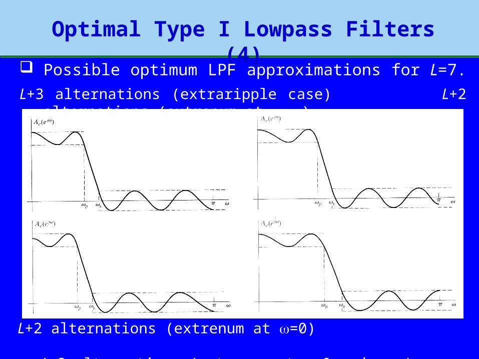
Optimal Type I Lowpass Filters (4)
Possible optimum LPF approximations for L=7.
L+3 alternations (extraripple case) L+2 alternations (extrenum at )
L+2 alternations (extrenum at =0) L+2 alternations (extrenum at =0 and )

19
Optimal Type I Lowpass Filters (5)
Illustrations supporting the second and third properties

20
Optimal Type II Lowpass Filters (1)
For type II filters, the filter length (M+1) is even, with the symmetric property
h[n]= h[M – n]
Therefore, the frequency response H(ej) can be expressed in the form
Let b[n]=2h[(M+1)/2 –n], n=1, 2, …, (M+1)/2, then
2/)1(
0
2/
2cos][2)(
M
n
Mjj nM
nheeH
2/)1(
0
2/
2/)1(
1
2/
)cos(][~
)2/cos(
2
1cos][)(
M
n
Mj
M
n
Mjj
nnbe
nnbeeH

21
Optimal Type II Lowpass Filters (2)
Derivation memo (see Problem 7.52)
Using the trigonometric identitycos cos = ½ cos(+) + ½ cos(–)
we get
2cos
2
1~
2
1
2cos]0[
~
2
1
2
1cos])[
~]1[
~(
2
1
2cos
2
1~
2
1
2cos]0[
~
2
1
2
1cos][
~
2
1
2
1cos]1[
~
2
1
2
1cos][
~
2
1
2
1cos][
~
2
1
)cos(][~
)2/cos(
2/)1(
1
2/)1(
1
2/)1(
1
2/)1(
0
2/)1(
0
2/)1(
0
MMbbnnbnb
MMbb
nnbnnb
nnbnnb
nnb
M
n
M
n
M
n
M
n
M
n
M
n
22
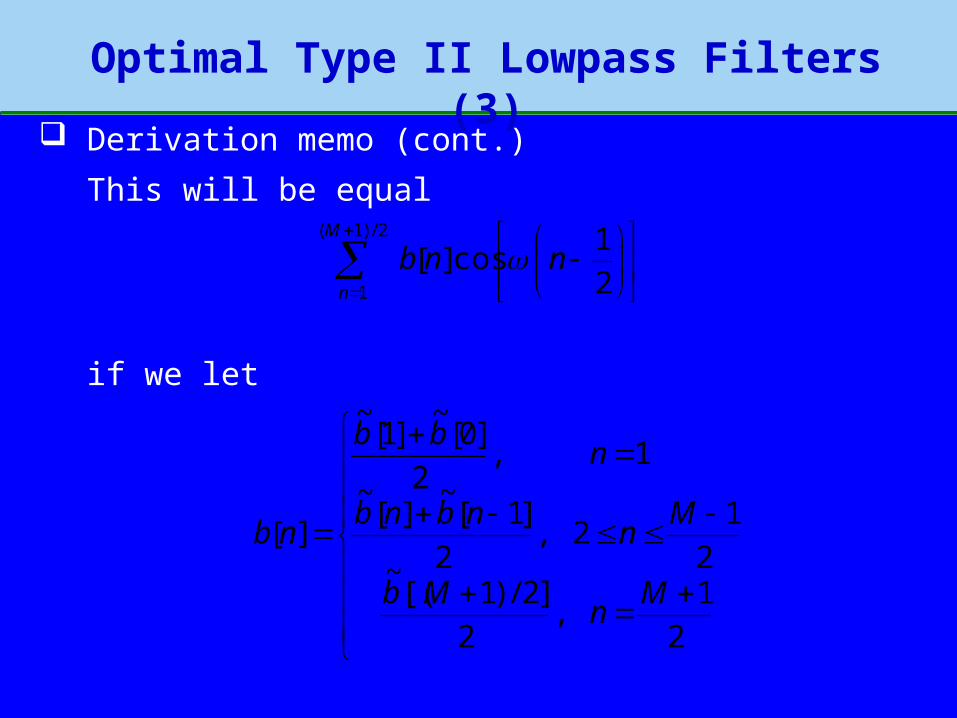
Optimal Type II Lowpass Filters (3)
Derivation memo (cont.)
This will be equal
if we let
2
1,
2
]2/)1[(~ 2
12,
2
]1[~
][~
1,2
]0[~
]1[~
][
Mn
Mb
Mn
nbnb
nbb
nb
2/)1(
1 2
1cos][
M
n
nnb
23
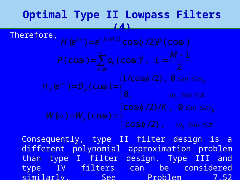
Optimal Type II Lowpass Filters (4)
Therefore,
Consequently, type II filter design is a different polynomial approximation problem than type I filter design. Type III and type IV filters can be considered similarly. See Problem 7.52 (http://www.ece.villanova.edu/~zhang/ECE8231/answer/solution752.pdf ).
2
1,)(cos)(cos
0
MLaP
L
k
kk
s
p
pj
d DeH,0
0),2/cos(/1)(cos)(
)(cos)2/cos()( 2/ PeeH Mjj
s
p
p
KWW
),2/cos(
0,/)2/cos()(cos)(
24
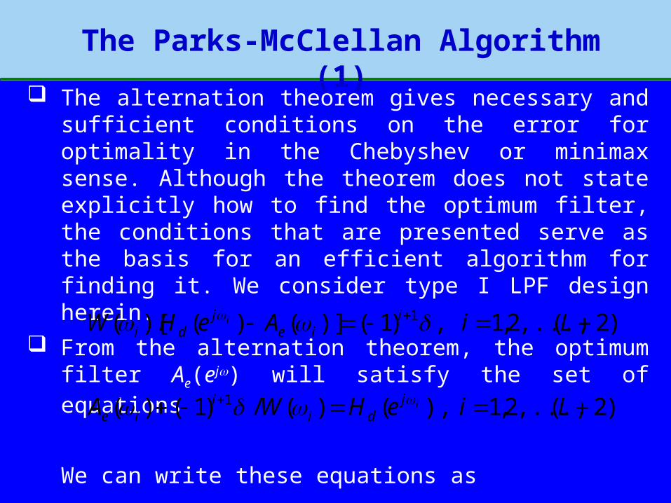
The Parks-McClellan Algorithm (1)
The alternation theorem gives necessary and sufficient conditions on the error for optimality in the Chebyshev or minimax sense. Although the theorem does not state explicitly how to find the optimum filter, the conditions that are presented serve as the basis for an efficient algorithm for finding it. We consider type I LPF design herein.
From the alternation theorem, the optimum filter Ae(ej) will satisfy the set of equations
We can write these equations as
)2(,...,2,1,)1()]()()[( 1 LiAeHW iie
jdi
i
)2(,...,2,1),()(/)1()( 1 LieHWA ijdi
iie

25
The Parks-McClellan Algorithm (2)
In matrix form, it becomes (xi=cos i)
This set of equations serves as the basis for an iterative algorithm for finding the optimum Ae(ej). The procedure begins by guessing a set of alternation frequencies i, i=1, 2, …, (L+2).
Note that p and s are fixed and are necessary members of the set of alternation frequencies. Specifically, if l = p,
then l+1= s.
)(
)(
)(
)(/)1(1
)(/11)(/11
2
2
1
1
0
22
222
22222
11211
Ljd
jd
jd
LLL
LLL
L
L
eH
eH
eHaa
Wxxx
WxxxWxxx

26
The Parks-McClellan Algorithm (3)
The above set of equations could be solved for the set of coefficients ak and .
A more efficient alternative is to use polynomial interpolation. In particular, Parks and McClellan found that, for the given set of the extremal frequencies (xi=cos i),
That is, Ae(ej) has values 1 K if 0 ≤ i ≤ p and if s ≤
≤ .
2
1
1
2
1
)(
)1(
)(
L
k k
kk
L
k
jdk
W
b
eHb k
2
1 )(
1L
kii ik
k xxb

27
The Parks-McClellan Algorithm (4)
Now, since Ae(ej) is known to be an Lth-order trigonometric polynomial, we can interpolate a trigonometric polynomial through (L+1) of the (L+2) known values E(i) [or, equivalently, Ae(ej)].
28
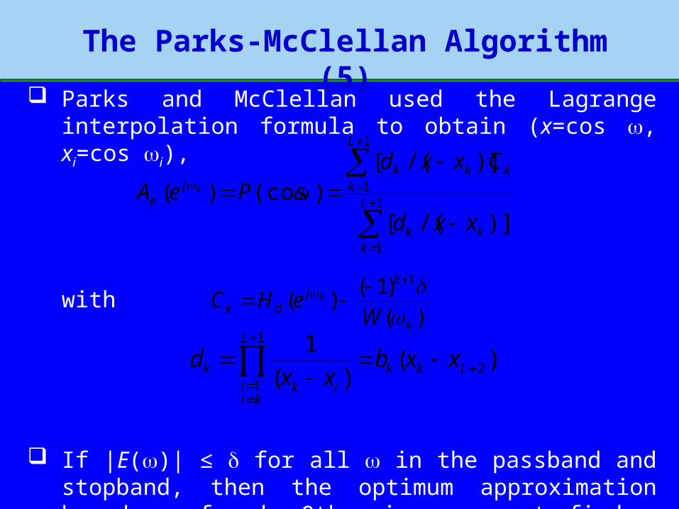
The Parks-McClellan Algorithm (5)
Parks and McClellan used the Lagrange interpolation formula to obtain (x=cos , xi=cos i),
with
If |E()| ≤ for all in the passband and stopband, then the optimum approximation has been found. Otherwise we must find a new set of extremal frequencies.
1
1
1
1
)]/([
)]/([)(cos)( L
kkk
L
kkkk
je
xxd
CxxdPeA k
)()(
12
1
1
Lkk
L
kii ik
k xxbxx
d
)(
)1()(
1
k
kj
dk WeHC k

29
The Parks-McClellan Algorithm (6)
For the LPF shown at the previous figure, was too small. The extremal frequencies are exchanged for a completely new set defined by the (L+2) largest peaks of the error curve (marked with x in the figure).
As before, p and s must be selected as extremal frequencies.
Also recall that there are at most (L –1) local minima and maxima in the open interval 0 < < p and s < < . The
remaining extrema can be either =0 and . If there is a maximum of the error function at both 0 and , then the frequency at which the greatest error occurs is taken as the new estimate of the frequency of the remaining extremum.
The circle – computing the value of , fitting a polynomial to the assumed error peaks, and then locating the actual error peaks – is repeating until does not change from its previous value by more than a prescribed small amount.
30
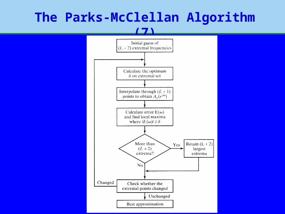
The Parks-McClellan Algorithm (7)
31
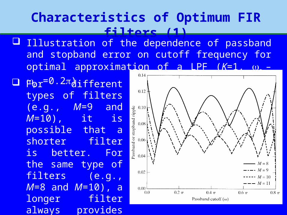
Characteristics of Optimum FIR filters (1)
For different types of filters (e.g., M=9 and M=10), it is possible that a shorter filter is better. For the same type of filters (e.g., M=8 and M=10), a longer filter always provides better or identical performance (in this case, the two filters are identical).
Illustration of the dependence of passband and stopband error on cutoff frequency for optimal approximation of a LPF (K=1, s – p =0.2).
32
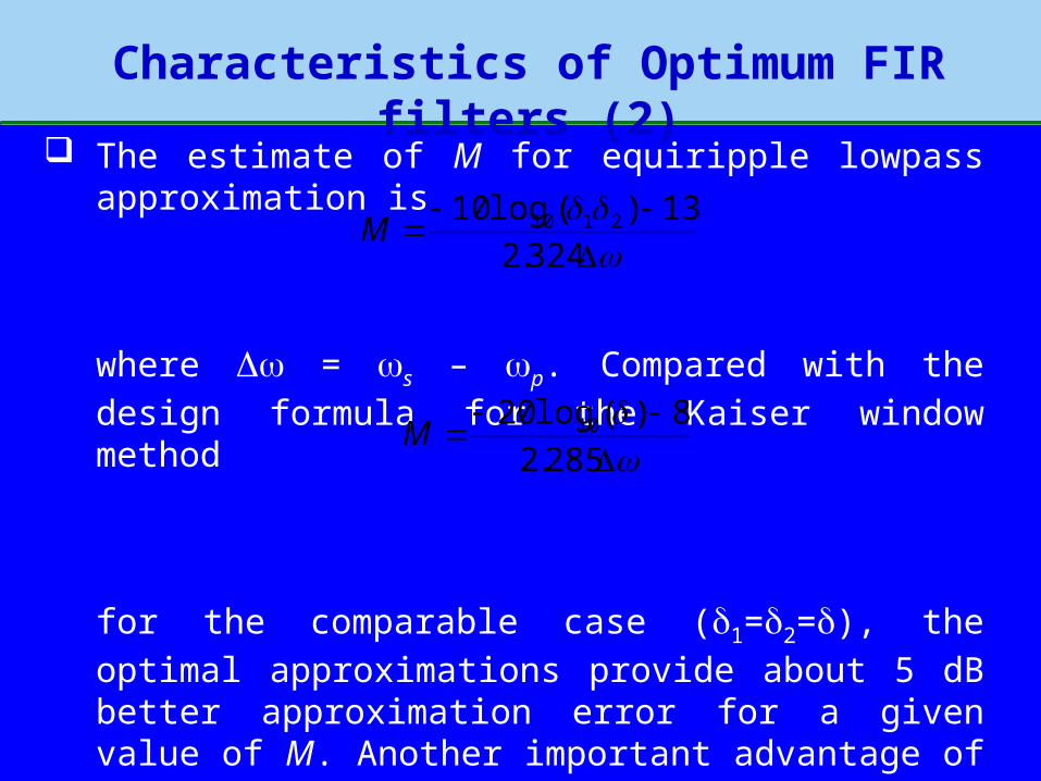
Characteristics of Optimum FIR filters (2)
The estimate of M for equiripple lowpass approximation is
where = s – p. Compared with the design formula for the
Kaiser window method
for the comparable case (1=2=), the optimal approximations
provide about 5 dB better approximation error for a given value of M. Another important advantage of equiripple filters is that 1 and 2 need not be equal, as must be the case for the window
method.
324.2
13)(log10 2110M
285.2
8)(log20 10M
33
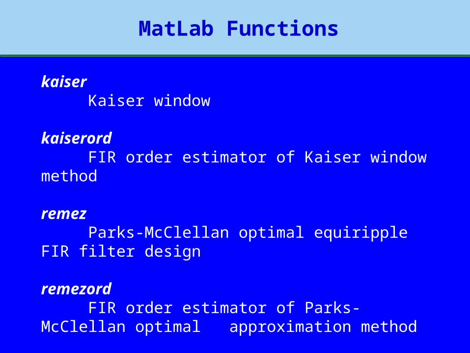
kaiser Kaiser window
kaiserordFIR order estimator of Kaiser window method
remezParks-McClellan optimal equiripple FIR filter design
remezordFIR order estimator of Parks-McClellan optimal
approximation method
MatLab Functions

34
Design Examples - LPF (1)
LPF Design Example
[1=0.01, 2=0.001, (K=10), ps ]
estimate of M=25.34 M=26, result: maximum error in the stopband = 0.00116: unsatisfied.
35
Design Examples - LPF (2)
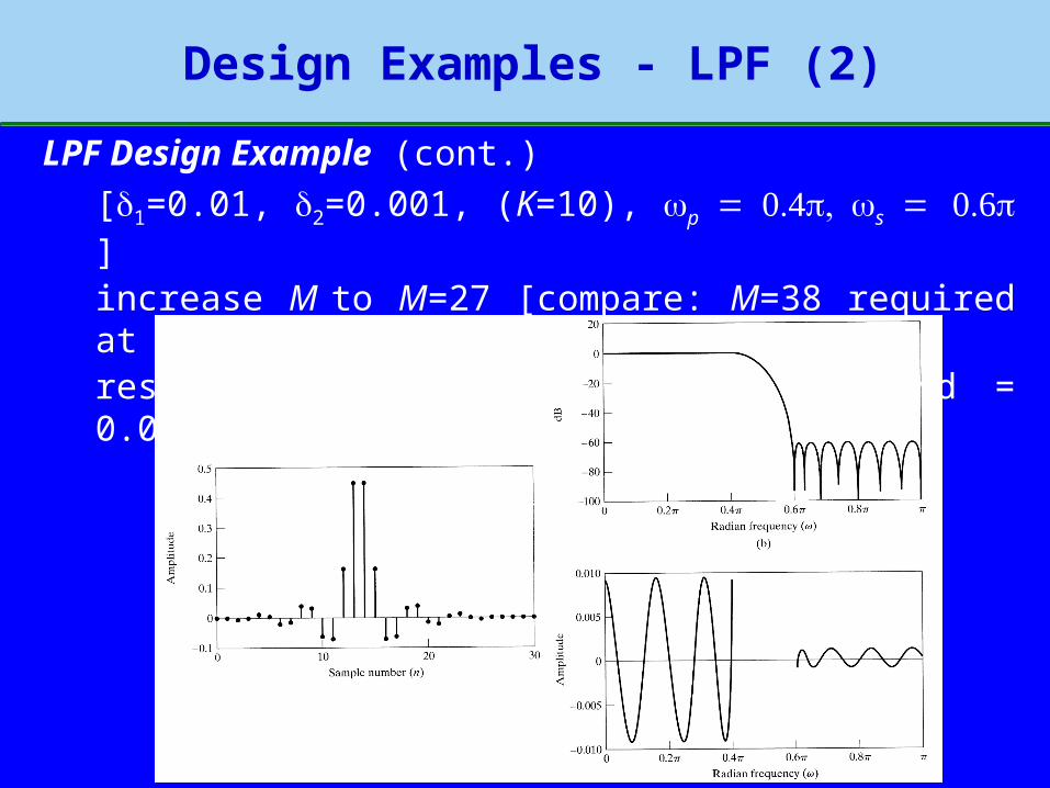
LPF Design Example (cont.)
[1=0.01, 2=0.001, (K=10), ps ]
increase M to M=27 [compare: M=38 required at Kaiser window]result: maximum error in the stopband = 0.00092: satisfactory.
36
Design Examples - BPF (1)
For an LPF filter, there are only two approximation bands. However, bandpass and bandstop filters require three approximation bands.
The alternation theorem does not assume any limit on the number of disjoint approximation intervals. Therefore, the minimum number of alternations is still (L+2). However, multiband filters can have more than (L+3) alternations, because there are more band edges.
Some of the statements so far are not true in the multiband case. For example, it is not necessary for all the local minima or maxima of Ae(ej) to lie inside the approximation intervals. Local extrema can occur in the transition regions, and the approximation need not be equiripple in the approximation regions.
37
Design Examples - BPF (2)
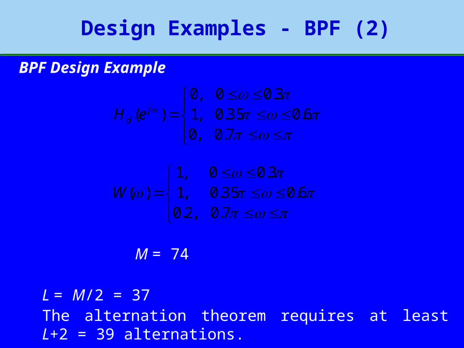
BPF Design Example
M = 74
L = M/2 = 37The alternation theorem requires at least L+2 = 39 alternations.
7.0,06.035.0,1
3.00,0)( j
d eH
7.0,2.06.035.0,1
3.00,1)(W

38
Design Examples - BPF (3)

39
Design Examples - BPF (4)
The approximations we obtained are optimal in the sense of the alternation theorem, but they would probably be unacceptable in a filtering application. In general, there is no guarantee that the transition region of a multiband filter will be monotonic, because the Parks-McClellan algorithm leaves these regions completely unconstrained.
When this kind of response results for a particularly choice of the filter parameters, acceptable transition regions can usually be obtained by systematically changing one or more of the band edge frequencies, the impulse-response length, or the error-weighting function and redesigning the filter.
40
Comments on IIR and FIR Filters
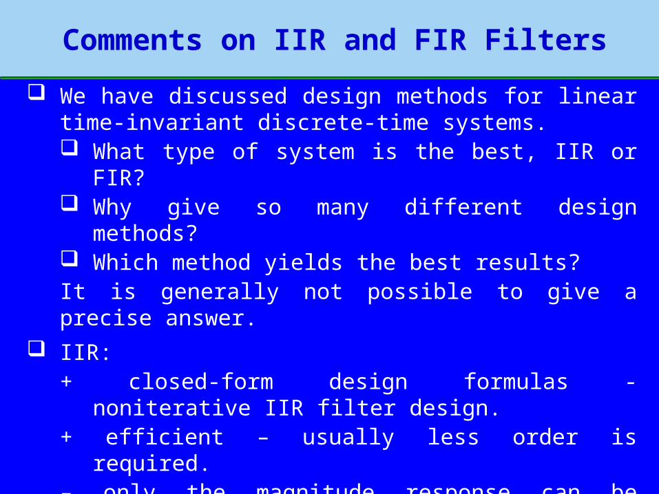
We have discussed design methods for linear time-invariant discrete-time systems. What type of system is the best, IIR or FIR? Why give so many different design methods? Which method yields the best results?It is generally not possible to give a precise answer.
IIR:+ closed-form design formulas - noniterative IIR filter design. + efficient – usually less order is required.– only the magnitude response can be specified.
FIR: + precise generalized linear phase.– no closed-form design formula - some iterations may be necessary to meet a given specification.

41
Homework Assignments (9)
7.8
7.36hint: The frequency response is not 0 at both
=0 and ;
Deadline : 6:00pm next Tuesday.