1

Chapter 6

Why Diversification Is a Good Idea

2

Introduction Diversification of a portfolio is logically a

good idea

Virtually all stock portfolios seek to diversify in one respect or another

3

Carrying Your Eggs in More Than One Basket

Investments in your own ego The concept of risk aversion revisited Multiple investment objectives

4

Investments in Your Own Ego Never put a large percentage of investment

funds into a single security• If the security appreciates, the ego is stroked

and this may plant a speculative seed• If the security never moves, the ego views this

as neutral rather than an opportunity cost• If the security declines, your ego has a very

difficult time letting go

5

The Concept of Risk Aversion Revisited

Diversification is logical• If you drop the basket, all eggs break

Diversification is mathematically sound• Most people are risk averse• People take risks only if they believe they will

be rewarded for taking them

6

The Concept of Risk Aversion Revisited (cont’d)

Diversification is more important now• Journal of Finance article shows that volatility

of individual firms has increased

– Investors need more stocks to adequately diversify

7

Multiple Investment Objectives Multiple objectives justify carrying your

eggs in more than one basket• Some people find mutual funds “unexciting”• Many investors hold their investment funds in

more than one account so that they can “play with” part of the total

– E.g., a retirement account and a separate brokerage account for trading individual securities

8

Lessons from Evans and Archer

Introduction Methodology Results Implications Words of caution

9

Introduction Evans and Archer’s 1968 Journal of

Finance article• Very consequential research regarding portfolio

construction

• Shows how naïve diversification reduces the dispersion of returns in a stock portfolio

– Naïve diversification refers to the selection of portfolio components randomly

10

Methodology Used computer simulations:

• Measured the average variance of portfolios of different sizes, up to portfolios with dozens of components

• Purpose was to investigate the effects of portfolio size on portfolio risk when securities are randomly selected

11

Results Definitions General results Strength in numbers Biggest benefits come first Superfluous diversification

12

Definitions Systematic risk is the risk that remains after

no further diversification benefits can be achieved

Unsystematic risk is the part of total risk that is unrelated to overall market movements and can be diversified• Research indicates up to 75 percent of total risk

is diversifiable

13

Definitions (cont’d) Investors are rewarded only for systematic

risk• Rational investors should always diversify

• Explains why beta (a measure of systematic risk) is important

– Securities are priced on the basis of their beta coefficients

14

General Results

Number of Securities

Portfolio Variance

15

Strength in Numbers Portfolio variance (total risk) declines as the

number of securities included in the portfolio increases• On average, a randomly selected ten-security

portfolio will have less risk than a randomly selected three-security portfolio

• Risk-averse investors should always diversify to eliminate as much risk as possible

16

Biggest Benefits Come First Increasing the number of portfolio

components provides diminishing benefits as the number of components increases• Adding a security to a one-security portfolio

provides substantial risk reduction

• Adding a security to a twenty-security portfolio provides only modest additional benefits

17

Superfluous Diversification Superfluous diversification refers to the

addition of unnecessary components to an already well-diversified portfolio• Deals with the diminishing marginal benefits of

additional portfolio components

• The benefits of additional diversification in large portfolio may be outweighed by the transaction costs

18

Implications Very effective diversification occurs when

the investor owns only a small fraction of the total number of available securities• Institutional investors may not be able to avoid

superfluous diversification due to the dollar size of their portfolios

– Mutual funds are prohibited from holding more than 5 percent of a firm’s equity shares

19

Implications (cont’d) Owning all possible securities would

require high commission costs

It is difficult to follow every stock

20

Words of Caution Selecting securities at random usually gives

good diversification, but not always Industry effects may prevent proper

diversification Although naïve diversification reduces risk,

it can also reduce return• Unlike Markowitz’s efficient diversification

21

Markowitz’s Contribution Harry Markowitz’s “Portfolio Selection” Journal

of Finance article (1952) set the stage for modern portfolio theory• The first major publication indicating the important of

security return correlation in the construction of stock portfolios

• Markowitz showed that for a given level of expected return and for a given security universe, knowledge of the covariance and correlation matrices are required

22

Quadratic Programming The Markowitz algorithm is an application

of quadratic programming• The objective function involves portfolio

variance

• Quadratic programming is very similar to linear programming

23

Portfolio Programming in A Nutshell

Various portfolio combinations may result in a given return

The investor wants to choose the portfolio combination that provides the least amount of variance

24

Markowitz Quadratic Programming Problem

25

Concept of Dominance Dominance is a situation in which investors

universally prefer one alternative over another• All rational investors will clearly prefer one

alternative

26

Concept of Dominance (cont’d) A portfolio dominates all others if:

• For its level of expected return, there is no other portfolio with less risk

• For its level of risk, there is no other portfolio with a higher expected return

27

Concept of Dominance (cont’d)Example (cont’d)

In the previous example, the B/C combination dominates the A/C combination:

0

0.02

0.04

0.06

0.08

0.1

0.12

0.14

0 0.005 0.01 0.015 0.02 0.025 0.03

Risk

Exp

ecte

d R

etu

rn

B/C combination dominates A/C

28

Terminology Security Universe Efficient frontier Capital market line and the market portfolio Security market line Expansion of the SML to four quadrants Corner portfolio

29

Security Universe The security universe is the collection of all

possible investments• For some institutions, only certain investments

may be eligible

– E.g., the manager of a small cap stock mutual fund would not include large cap stocks

30

Efficient Frontier Construct a risk/return plot of all possible

portfolios• Those portfolios that are not dominated

constitute the efficient frontier

31

Efficient Frontier (cont’d)

Standard Deviation

Expected Return100% investment in security with highest E(R)

100% investment in minimum variance portfolio

Points below the efficient frontier are dominated

No points plot above the line

All portfolios on the line are efficient

32

Efficient Frontier (cont’d) When a risk-free investment is available,

the shape of the efficient frontier changes• The expected return and variance of a risk-free

rate/stock return combination are simply a weighted average of the two expected returns and variance

– The risk-free rate has a variance of zero

33

Efficient Frontier (cont’d)

Standard Deviation

Expected Return

Rf A

B

C

34

Efficient Frontier (cont’d) The efficient frontier with a risk-free rate:

• Extends from the risk-free rate to point B– The line is tangent to the risky securities efficient

frontier

• Follows the curve from point B to point C

35

Theorem For any constant Rf on the returns axis, the

weights of the tangency portfolio B are:

11

1 1

, , where z is given by: [ ]

In other words, the weights of tangency portfolio B are the normalized

weights of portfolio z.

nfn n

j jj j

zzz V R

z z

36

Example with Rf=0 and Rf=6.5%

23456789101112131415161718

A B C D E F G H I J

MeanMean minus

Variance-covariance matrix returns constant0.400 0.030 0.020 0.000 0.06 -0.005 <-- =F6-$E$110.030 0.200 0.001 -0.060 0.05 -0.015 <-- =F7-$E$110.020 0.001 0.300 0.030 0.07 0.005 <-- =F8-$E$110.000 -0.060 0.030 0.100 0.08 0.015 <-- =F9-$E$11

Rf= 0.00 Rf= 0.065z B z B

0.1019 0.0540 -0.0101 -0.11630.5657 0.2998 -0.0353 -0.40670.1141 0.0605 0.0047 0.05441.1052 0.5857 0.1274 1.4687

Cells E13:E16 contain the array function =MMULT(MINVERSE(A6:D9),G6:G9). Cell F13 contains the function=E13/SUM($E$13:$E$16). This function is copied to cells F14:F16.

37

Graphically:Finding Envelope Portfolios

0%

2%

4%

6%

8%

10%

12%

0% 10% 20% 30% 40% 50% 60% 70% 80% 90%

Portfolio standard deviation

Po

rtfo

lio

me

an r

etu

rn

Rf

B, the tangency portfolio given Rf

Zero beta portfolio

38

What is the zero-beta portfolio? The zero beta portfolio P0 is the portfolio

determined by the intersection of the frontier with a horizontal line originating from the constant Rf selected.

Property: whatever Rf we choose, we always have Cov(B,P0)=0

(Notice, however, that the location of B and P0 will depend on the value selected for Rf)

39

Note that the last proposition is true even if the risk-free rate (i.e. a riskless security) doesn’t exist in the economy.

The way the tangency portfolio B was determined also remains valid even if there is no riskless rate in the economy.

All one has to do is replace Rf by a chosen constant c. The mathematics of the last propositions will remain valid.

40

Fisher Black zero beta CAPM (1972)

For a chosen constant c on the vertical axis of returns, the tangency portfolio B can be computed, and for ANY portfolio x we have a linear relationship if we regress the returns of x on the returns of B:

Moreover, c is the expected rate of return of a portfolio P0 whose covariance with B is zero.

2( ) [ ( ) ] where ( , ) /x x B x BE R c E R c Cov x B

0 0( ) and ( , ) 0Pc E R Cov P B

41

Fisher Black zero beta CAPM (Cont’d)

The name “zero beta” stems from the fact that the covariance between P0 and B is zero, since a zero covariance implies that the beta of P0 with respect to B is zero too.

If a riskless asset DOES exist in the economy, however, we can replace the constant c in Black’s zero beta CAPM by Rf

and the portfolio B is the market portfolio.

42

Capital Market Line and the Market Portfolio

The tangent line passing from the risk-free rate through point B is the capital market line (CML)• When the security universe includes all possible

investments, point B is the market portfolio– It contains every risky assets in the proportion of its

market value to the aggregate market value of all assets– It is the only risky assets risk-averse investors will hold

43

Capital Market Line and the Market Portfolio (cont’d)

Implication for investors:• Regardless of the level of risk-aversion, all

investors should hold only two securities:– The market portfolio– The risk-free rate

• Conservative investors will choose a point near the lower left of the CML

• Growth-oriented investors will stay near the market portfolio

44

Capital Market Line and the Market Portfolio (cont’d)

Any risky portfolio that is partially invested in the risk-free asset is a lending portfolio

Investors can achieve portfolio returns greater than the market portfolio by constructing a borrowing portfolio

45

Capital Market Line and the Market Portfolio (cont’d)

Standard Deviation

Expected Return

Rf A

B

C

46

Security Market Line The graphical relationship between

expected return and beta is the security market line (SML)• The slope of the SML is the market price of

risk

• The slope of the SML changes periodically as the risk-free rate and the market’s expected return change

47

Security Market Line (cont’d)

Beta

Expected Return

Rf

Market Portfolio

1.0

E(R)

48

123456789101112131415161718192021

A B C D E F G H I J K L M N O

AMR BS GE HR MO UK SP500 Regressing the means on the betas:1974 -0.3505 -0.1154 -0.4246 -0.2107 -0.0758 0.2331 -0.2647 Intercept 0.07659 <-- =INTERCEPT(B15:G15,B16:G16)1975 0.7083 0.2472 0.3719 0.2227 0.0213 0.3569 0.3720 Slope 0.054509 <-- =SLOPE(B15:G15,B16:G16)1976 0.7329 0.3665 0.2550 0.5815 0.1276 0.0781 0.2384 R-squared 0.279317 <-- =RSQ(B15:G15,B16:G16)1977 -0.2034 -0.4271 -0.0490 -0.0938 0.0712 -0.2721 -0.07181978 0.1663 -0.0452 -0.0573 0.2751 0.1372 -0.1346 0.06561979 -0.2659 0.0158 0.0898 0.0793 0.0215 0.2254 0.1844 Mean Beta1980 0.0124 0.4751 0.3350 -0.1894 0.2002 0.3657 0.3242 0.203227 1.4820381981 -0.0264 -0.2042 -0.0275 -0.7427 0.0913 0.0479 -0.0491 0.053134 1.0839761982 1.0642 -0.1493 0.6968 -0.2615 0.2243 0.0456 0.2141 0.150107 1.3106731983 0.1942 0.3680 0.3110 1.8682 0.2066 0.2640 0.2251 0.152874 1.299112

0.102546 0.262246Mean 0.2032 0.0531 0.1501 0.1529 0.1025 0.1210 0.1238 0.120996 0.493903Beta 1.4820 1.0840 1.3107 1.2991 0.2622 0.4939 1.0000

=SLOPE(B4:B13,$H$4:$H$13)=COVAR(B4:B13,$H$4:$H$13)/VARP($H$4:$H$13)

THE SECURITY MARKET LINE--A SIMPLE EXAMPLE

49

Notice that we obtained very poor results. The R-squared is only 27.93% !

However, the math of the CAPM is undoubtedly true.

How then can CAPM fail in the real world? Possible explanations are that true asset

returns distributions are unobservable, individuals have non-homogenous expectations, the market portfolio is unobservable, the riskless rate is ambiguous, markets are not friction-free.

50

Efficient Portfolios Showing the S&P 500 Portfolio

0%

5%

10%

15%

20%

25%

30%

0% 5% 10% 15% 20% 25%

Sigma

Mea

n r

etu

rn

S&P 500

51

Using “Artificial Market Portfolio”474849505152535455565758596061626364656667686970

D E F G H I J K LANNUAL RETURNS ON SIX ASSETS AND "MARKET" PORTFOLIO

"Market" AMR BS GE HR MO UK portfolio

1974 -0.3505 -0.1154 -0.4246 -0.2107 -0.0758 0.2331 0.35601975 0.7083 0.2472 0.3719 0.2227 0.0213 0.3569 0.38451976 0.7329 0.3665 0.2550 0.5815 0.1276 0.0781 0.01891977 -0.2034 -0.4271 -0.0490 -0.0938 0.0712 -0.2721 0.15581978 0.1663 -0.0452 -0.0573 0.2751 0.1372 -0.1346 0.08721979 -0.2659 0.0158 0.0898 0.0793 0.0215 0.2254 0.20701980 0.0124 0.4751 0.3350 -0.1894 0.2002 0.3657 -0.11211981 -0.0264 -0.2042 -0.0275 -0.7427 0.0913 0.0479 0.23401982 1.0642 -0.1493 0.6968 -0.2615 0.2243 0.0456 0.55501983 0.1942 0.3680 0.3110 1.8682 0.2066 0.2640 0.3918

Mean 0.2032 0.0531 0.1501 0.1529 0.1025 0.1210 0.2278Beta with respect to "market"

0.7938 -0.4647 0.3484 0.3716 -0.0504 0.1043 1.0000

=SLOPE(E50:E59,$L$50:$L$59)

Regressing the means on the betasIntercept 0.1086 <-- =INTERCEPT(E61:J61,E63:J63)Slope 0.1193 <-- =SLOPE(E61:J61,E63:J63)R-squared 1.0000 <-- =RSQ(E61:J61,E63:J63)

52

We obtained a perfect 100% R-squared this time !

The reason is that when portfolio returns are regressed on their betas with respect to an efficient portfolio, an exact linear relationship holds.

53

Expansion of the SML to Four Quadrants

There are securities with negative betas and negative expected returns• A reason for purchasing these securities is their

risk-reduction potential– E.g., buy car insurance without expecting an

accident

– E.g., buy fire insurance without expecting a fire

54

Security Market Line (cont’d)

Beta

Expected Return

Securities with NegativeExpected Returns

55

Diversification and Beta Beta measures systematic risk

• Diversification does not mean to reduce beta• Investors differ in the extent to which they will

take risk, so they choose securities with different betas

– E.g., an aggressive investor could choose a portfolio with a beta of 2.0

– E.g., a conservative investor could choose a portfolio with a beta of 0.5

56

Capital Asset Pricing Model Introduction Systematic and unsystematic risk Fundamental risk/return relationship

revisited

57

Introduction The Capital Asset Pricing Model (CAPM)

is a theoretical description of the way in which the market prices investment assets• The CAPM is a positive theory

58

Systematic and Unsystematic Risk

Unsystematic risk can be diversified and is irrelevant

Systematic risk cannot be diversified and is relevant• Measured by beta

– Beta determines the level of expected return on a security or portfolio (SML)

59

CAPM The more risk you carry, the greater the

expected return:

( ) ( )

where ( ) expected return on security

risk-free rate of interest

beta of Security

( ) expected return on the market

i f i m f

i

f

i

m

E R R E R R

E R i

R

i

E R

60

CAPM (cont’d) The CAPM deals with expectations about

the future

Excess returns on a particular stock are directly related to:• The beta of the stock• The expected excess return on the market

61

CAPM (cont’d) CAPM assumptions:

• Variance of return and mean return are all investors care about

• Investors are price takers– They cannot influence the market individually

• All investors have equal and costless access to information

• There are no taxes or commission costs

62

CAPM (cont’d) CAPM assumptions (cont’d):

• Investors look only one period ahead

• Everyone is equally adept at analyzing securities and interpreting the news

63

SML and CAPM If you show the security market

line with excess returns on the vertical axis, the equation of the SML is the CAPM • The intercept is zero

• The slope of the line is beta

64

Note on the CAPM Assumptions

Several assumptions are unrealistic:• People pay taxes and commissions

• Many people look ahead more than one period

• Not all investors forecast the same distribution

Theory is useful to the extent that it helps us learn more about the way the world acts• Empirical testing shows that the CAPM works

reasonably well

65

Stationarity of Beta Beta is not stationary

• Evidence that weekly betas are less than monthly betas, especially for high-beta stocks

• Evidence that the stationarity of beta increases as the estimation period increases

The informed investment manager knows that betas change

66

Equity Risk Premium Equity risk premium refers to the

difference in the average return between stocks and some measure of the risk-free rate• The equity risk premium in the CAPM is the

excess expected return on the market

• Some researchers are proposing that the size of the equity risk premium is shrinking

67

Using A Scatter Diagram to Measure Beta

Correlation of returns Linear regression and beta Importance of logarithms Statistical significance

68

Correlation of Returns Much of the daily news is of a general

economic nature and affects all securities• Stock prices often move as a group

• Some stock routinely move more than the others regardless of whether the market advances or declines

– Some stocks are more sensitive to changes in economic conditions

69

Linear Regression and Beta To obtain beta with a linear regression:

• Plot a stock’s return against the market return

• Use Excel to run a linear regression and obtain the coefficients

– The coefficient for the market return is the beta statistic

– The intercept is the trend in the security price returns that is inexplicable by finance theory

70

Importance of Logarithms Taking the logarithm of returns reduces the

impact of outliers• Outliers distort the general relationship

• Using logarithms will have more effect the more outliers there are

71

Statistical Significance Published betas are not always useful

numbers• Individual securities have substantial

unsystematic risk and will behave differently than beta predicts

• Portfolio betas are more useful since some unsystematic risk is diversified away

72

Arbitrage Pricing Theory APT background The APT model Comparison of the CAPM and the APT

73

APT Background Arbitrage pricing theory (APT) states that a

number of distinct factors determine the market return• Roll and Ross state that a security’s long-run

return is a function of changes in:– Inflation– Industrial production– Risk premiums– The slope of the term structure of interest rates

74

APT Background (cont’d) Not all analysts are concerned with the

same set of economic information• A single market measure such as beta does not

capture all the information relevant to the price of a stock

75

The APT Model General representation of the APT model:

1 1 2 2 3 3 4 4( )

where actual return on Security

( ) expected return on Security

sensitivity of Security to factor

unanticipated change in factor

A A A A A A

A

A

iA

i

R E R b F b F b F b F

R A

E R A

b A i

F i

76

APT1 1 2 2 3 3

1 1 1 2 2 2 3 3 3

1 1 2 2 3 3 1 1 2 2 3 3

Fixed Random

(Notice that the security index "A" has been ign

( )

( ) [ ( )] [ ( )] [ ( )]

( ) ( ) ( ) ( )

R E R F F F

R E R R E R R E R R E R

R E R E R E R E R R R R

ored for clarity purposes)

77

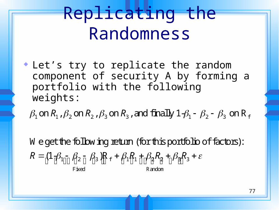
Replicating the Randomness

Let’s try to replicate the random component of security A by forming a portfolio with the following weights:

1 1 2 2 3 3 1 2 3 f

1 2 3 f 1 1 2 2 3 3

Fixed Random

on , on , on , and finally 1- on R

We get the following return (for this portfolio of factors):

(1- )R

R R R

R R R R

78

Key Point in Reasoning Since we were able to match the random

components exactly, the only terms that differ at this point are the fixed components.

But if one fixed component is larger than the other, arbitrage profits are possible by investing in the highest yielding security (either A or the portfolio of factors) while short-selling the other (being “long” in one and “short” in the other will assure an exact cancellation of the random terms).

79

Therefore the fixed components MUST BE THE SAME for security A and the portfolio of factors created, otherwise unlimited profits would be possible.

So we have:

1 1 2 2 3 3 1 2 3 f

f 1 1 f 2 2 f 2 3 f

( ) ( ) ( ) ( ) (1- )R

Rearranging terms yields:

( ) R [ ( ) R ] [ ( ) R ] [ ( ) R ]

E R E R E R E R

E R E R E R E R

80

Comparison of the CAPM and the APT

The CAPM’s market portfolio is difficult to construct:• Theoretically all assets should be included (real estate,

gold, etc.)

• Practically, a proxy like the S&P 500 index is used

APT requires specification of the relevant macroeconomic factors

81

Comparison of the CAPM and the APT (cont’d)

The CAPM and APT complement each other rather than compete• Both models predict that positive returns will

result from factor sensitivities that move with the market and vice versa