Embed Size (px)
Citation preview

1
Chapter 6
Autocorrelation
2
What is in this Chapter?
• How do we detect this problem?
• What are the consequences?
• What are the solutions?

3
What is in this Chapter?
• Regarding the problem of detection, we start with the
Durbin-Watson (DW) statistic, and discuss its several
limitations and extensions.
– Durbin's h-test for models with lagged dependent variables
– Tests for higher-order serial correlation.
• We discuss (in Section 6.5) the consequences of serially
correlated errors and OLS estimators.

4
What is in this Chapter?
• The solutions to the problem of serial correlation are
discussed in:
– Section 6.3: estimation in levels versus first differences
– Section 6.9: strategies when the DW test statistic is significant
– Section 6.10: trends and random walks
• This chapter is very important and the several ideas
have to be understood thoroughly.

5
6.1 Introduction
• The order of autocorrelation
• In the following sections we discuss how to:
1. Test for the presence of serial correlation.
2. Estimate the regression equation when the er
rors are serially correlated.

6
6.2 Durbin-Watson Test
n
t
n
tt
u
uud
1
2
2
21
ˆ
)ˆˆ(
2
12
12
ˆ
ˆˆ2ˆˆ
t
tttt
u
uuuud

7
6.2 Durbin-Watson Test
• The sampling distribution of d depends on values
of the explanatory variables and hence Durbin
and Watson derived upper limits and lower
limits for the significance level for d.
• There are tables to test the hypothesis of zero
autocorrelation against the hypothesis of first-
order positive autocorrelation. ( For negative
autocorrelation we interchange .)
)( Ud
)( Ld
UL dd and

8
6.2 Durbin-Watson Test
• If , we reject the null hypothesis of no
autocorrelation.
• If , we do not reject the null hypothesis.
• If , the test is inconclusive.
Ldd
Udd
UL ddd

9
6.2 Durbin-Watson Test
Illustrative Example
• Consider the data in Table 3.11. The estimated production function is
• Referring to the DW table with k’=2 and n=39 for 5% significance level, we see that .
• Since the observed , we reject the hypothesis at the 5% level.
559.0ˆ88.0DW9946.0
log384.0log451.1938.3log
2
1)048.0(
1)083.0()237.0(
R
KLX
38.1Ld
Ldd 858.00

10
6.2 Limitations of D-W Test
1. It test for only first-order serial correlation.
2. The test is inconclusive if the computed value
lies between .
3. The test cannot be applied in models with
lagged dependent variables.
UL dd and

11
6.3 Estimation in Levels Versus First Differences
• Simple solutions to the serial correlation problem: First
Difference
• If the DW test rejects the hypothesis of zero serial
correlation, what is the next step?
• In such cases one estimates a regression by
transforming all the variables by
– ρ-differencing (quasi-first difference)
– First-difference

12
6.3 Estimation in Levels Versus First Differences
)()()( 111
111
tttttt
ttt
ttt
uuxxyy
uxy
uxy

13
6.3 Estimation in Levels Versus First Differences
)()()(
)1(
111
111
tttttt
ttt
ttt
uuxxyy
uxty
uxty
14
6.3 Estimation in Levels Versus First Differences
• When comparing equations in levels and first
differences, one cannot compare the R2 because
the explained variables are different.
• One can compare the residual sum of squares
but only after making a rough adjustment.
(Please refer to P.231)

15
6.3 Estimation in Levels Versus First Differences
• Let from the first difference equation residual sum of squares from the levels equation residual sum of squares from the first difference
equation comparable from the levels equation
Then
221 RR
0RSS
1RSS
2DR
2R
dkn
kn
RSS
RSS
RSSdknkn
RSSR
R D
1
1
1
1
1
0
1021
2
16
6.3 Estimation in Levels Versus First Differences
Illustrative Examples
• Consider the simple Keynesian model discussed by Fri
edman and Meiselman. The equation estimated in leve
ls is
where Ct= personal consumption expenditure (current dollars)
At= autonomous expenditure (current dollars)
TtAC ttt ,....,2,1

17
6.3 Estimation in Levels Versus First Differences
• The model fitted for the 1929-1030 period gave (figures in parentheses are standard)
40
20
)324.0(
41
21
)312.0(
10387,851.18096.0
993.1.2
10943,1189.08771.0
4984.20.335,58.1
RSSDWR
AC
RSSDWR
AC
tt
tt

18
6.3 Estimation in Levels Versus First Differences
• This is to be compared with from the equation in first differences.
7828.02172.01
)8096.01()89.0(10
9
387.8
943.111
)1(1
1 21
1
02
Rdkn
kn
RSS
RSSRD
8096.021 R

19
6.3 Estimation in Levels Versus First Differences
• For the production function data in Table 3.11 the first difference equation is
• The comparable figures the levels equation reported earlier in Chapter 4, equation (4.24) are
0278.0177.18405.0
log502.0log987.0log
12
1
1)134.0(
1)158.0(
RSSDWR
KLX
0434.0858.09946.0 020 RSSDWR

20
6.3 Estimation in Levels Versus First Differences
• This is to be compared with from the equation in first differences.
7921.02079.01
)8405.01()858.0(37
36
0278.0
0434.012
DR
8405.021 R

21
6.3 Estimation in Levels Versus First Differences
• Harvey gives a different definition of .He defines it as
• This does not adjust for the fact that the error variances in the levels equations and the first difference equation are not the same.
• The arguments for his suggestion are given in his paper.
21
1
02 1 RRSS
RSSR D
2DR

22
6.3 Estimation in Levels Versus First Differences
• Usually, with time-series data, one gets high R2
values if the regressions are estimated with the l
evels yt and Xt but one gets low R2 values if the r
egressions are estimated in first differences (yt -
yt-1) and (xt - xt-1).

23
6.3 Estimation in Levels Versus First Differences
• Since a high R2 is usually considered as proof of
a strong relationship between the variables
under investigation, there is a strong tendency to
estimate the equations in levels rather than in
first differences.
• This is sometimes called the “R2 syndrome."
• An example

24
6.3 Estimation in Levels Versus First Differences
• However, if the DW statistic is very low, it often i
mplies a misspecified equation, no matter what t
he value of the R2 is
• In such cases one should estimate the regressio
n equation in first differences and if the R2 is low,
this merely indicates that the variables y and x ar
e not related to each other.

25
6.3 Estimation in Levels Versus First Differences
• Granger and Newbold present some examples with artificially generated data where y, x, and the error u are each generated independently so that there is no relationship between y and x.
• But the correlations between yt and yt-1,.Xt and Xt-1,
and ut and ut-1 are very high.
• Although there is no relationship between y and x the regression of y on x gives a high R2 but a low DW statistic.

26
6.3 Estimation in Levels Versus First Differences
• When the regression is run in first differences, the R2 is
close to zero and the DW statistic is close to 2.
• Thus demonstrating that there is indeed no relationship
between y and x and that the R2 obtained earlier is
spurious.
• Thus regressions in first differences might often reveal
the true nature of the relationship between y and x.
• An example

27
Homework• Find the data
– Y is the Taiwan stock index– X is the U.S. stock index
• Run two equations– The equation in levels (log-based price)– The equation in the first differences
• A comparison between the two equations– The beta estimate and its significance– The R square– The value of DW statistic
• Q: Adopt the equation in levels or the first differences?

28
6.3 Estimation in Levels Versus First Differences
• For instance, suppose that we have quarterly data; t
hen it is possible that the errors in any quarter this y
ear are most highly correlated with the errors in the
corresponding quarter last year rather than the error
s in the preceding quarter
• That is, ut could be uncorrelated with ut-1 but it could
be highly correlated with ut-4.
• If this is the case, the DW statistic will fail to detect it.

29
6.3 Estimation in Levels Versus First Differences
• What we should be using is a modified statistic defined as
• The quarterly data (e.g. GDP)
• The monthly data (e.g. Industrial product index)
2
24
4 ˆ
)ˆˆ(
t
tt
u
uud

30
6.4 Estimation Procedures with Autocorrelated Errors
• GLS (Generalized least squares)
),0(~,
)2.6(,......,2,12
1 etttt
ttt
eeuu
Ttuxy
iid

31
6.4 Estimation Procedures with Autocorrelated Errors
1*
1*
11
111
)6.6(,....,3,2
)5.6()()1(
)4.6(
ttt
ttt
ttttt
ttt
xxx
Ttyyy
exxyy
uxy

32
6.4 Estimation Procedures with Autocorrelated Errors
• In actual practice is not known
• There are two types of procedures for estimating – 1. Iterative procedures– 2. Grid-search procedures.
33
6.4 Estimation Procedures with Autocorrelated Errors
Iterative Procedures
• Among the iterative procedures, the earliest was
the Cochrane-Orcutt (C-O) procedure.
• In the Cochrane-Otcutt procedure we estimate e
quation(6.2) by OLS, get the estimated residuals
, and estimate .tu 21-tt ˆ/uuˆby tu

34
6.4 Estimation Procedures with Autocorrelated Errors
• Durbin suggested an alternative method of
estimating .
• In this procedure, we write equation (6.5) as
• We regress and take the
estimated coefficient of as an estimate of .
)7.6()1( 11 ttttt exxyy
11 and,, tttt xxyony
1ty
35
6.4 Estimation Procedures with Autocorrelated Errors
• Use equation (6.6) and (6.6’) and estimate a
regression of y* on x*.
• The only thing to note is that the slop coefficient
in this equation is , but the intercept is .
• Thus after estimating the regression of y* on x*,
we have to adjust the constant term
appropriately to get estimates of the parameters
of the original equation (6.2).
)1(

36
6.4 Estimation Procedures with Autocorrelated Errors
• Further, the standard errors we compute from the
regression of y* on x* are now ”asymptotic” standard
errors because of the fact that has been
estimated.
• If there are lagged values of y as explanatory
variables, these standard errors are not correct
even asymptotically.
• The adjustment needed in this case is discussed in
Section 6.7.

37
6.4 Estimation Procedures with Autocorrelated Errors
Grid-Search Procedures
• One of the first grid-search procedures is the Hil
dreth and Lu procedure suggested in 1960.
• The procedure is as follows. Calculate i
n equation(6.6) for different values of at interv
als of 0.1 in the rang .
• Estimate the regression of and calculate
the residual sum of squares RSS in each case.
** and tt xy
11 ** o tt xny
38
6.4 Estimation Procedures with Autocorrelated Errors
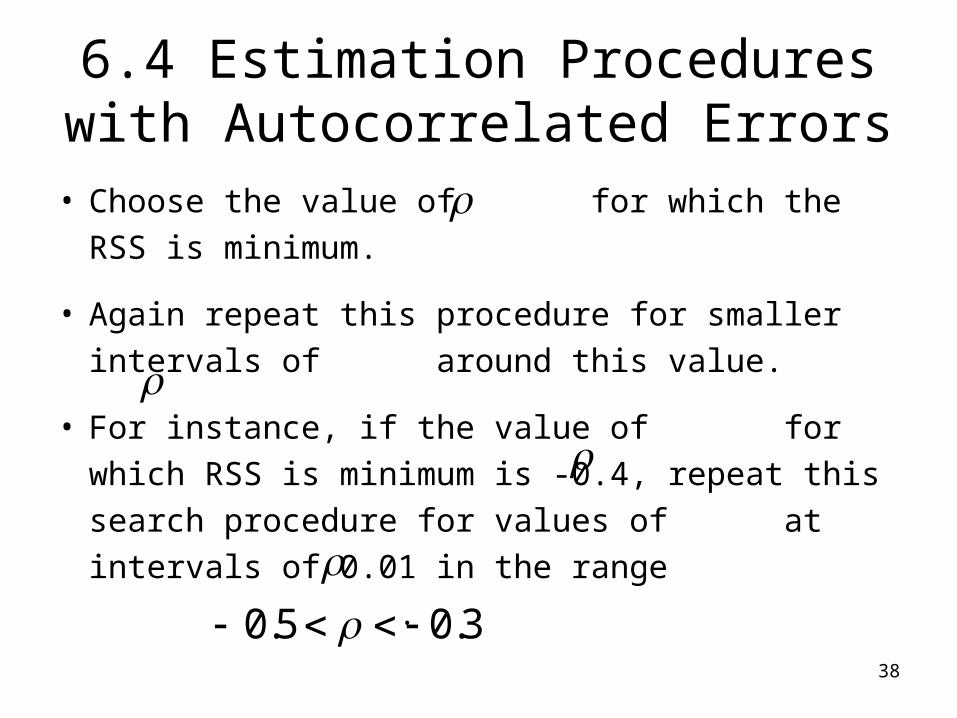
• Choose the value of for which the RSS is
minimum.
• Again repeat this procedure for smaller intervals
of around this value.
• For instance, if the value of for which RSS is
minimum is -0.4, repeat this search procedure
for values of at intervals of 0.01 in the range
.
3.05.0
39
6.4 Estimation Procedures with Autocorrelated Errors
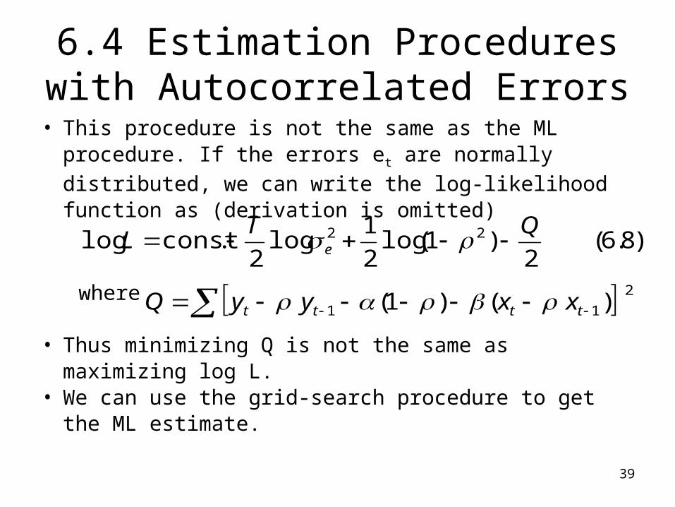
• This procedure is not the same as the ML procedure. If the errors et are normally distributed, we can write the
log-likelihood function as (derivation is omitted)
where
• Thus minimizing Q is not the same as maximizing log L. • We can use the grid-search procedure to get the ML
estimate.
)8.6(2
)1(log2
1log
2.constlog 22 QT
L e
2
11 )()1( tttt xxyyQ

40
6.4 Estimation Procedures with Autocorrelated Errors
• Consider the data in Table 3.11 and the estimation of the production function
• The OLS estimation gave a DW statistic of 0.86, suggesting significant positive autocorrelation.
• Assuming that the errors were AR(1), two estimation procedures were used: the Hildreth-Lu grid search and the iterative Cochrane-Orcutt (C-O).
uKLX 1211 logloglog

41
6.4 Estimation Procedures with Autocorrelated Errors
• The Hildreth-Lu procedure gave .
• The iterative C-O procedure gave
.
• The DW test statistic implied that
.
77.0ˆ
80.0ˆ
57.0)86.02)(2/1(ˆ

42
6.4 Estimation Procedures with Autocorrelated Errors
• The estimates of the parameters (with standard errors in parentheses) were as follows:

43
6.5 Effect of AR(1) Errors on OLS Estimates
44
6.5 Effect of AR(1) Errors on OLS Estimates
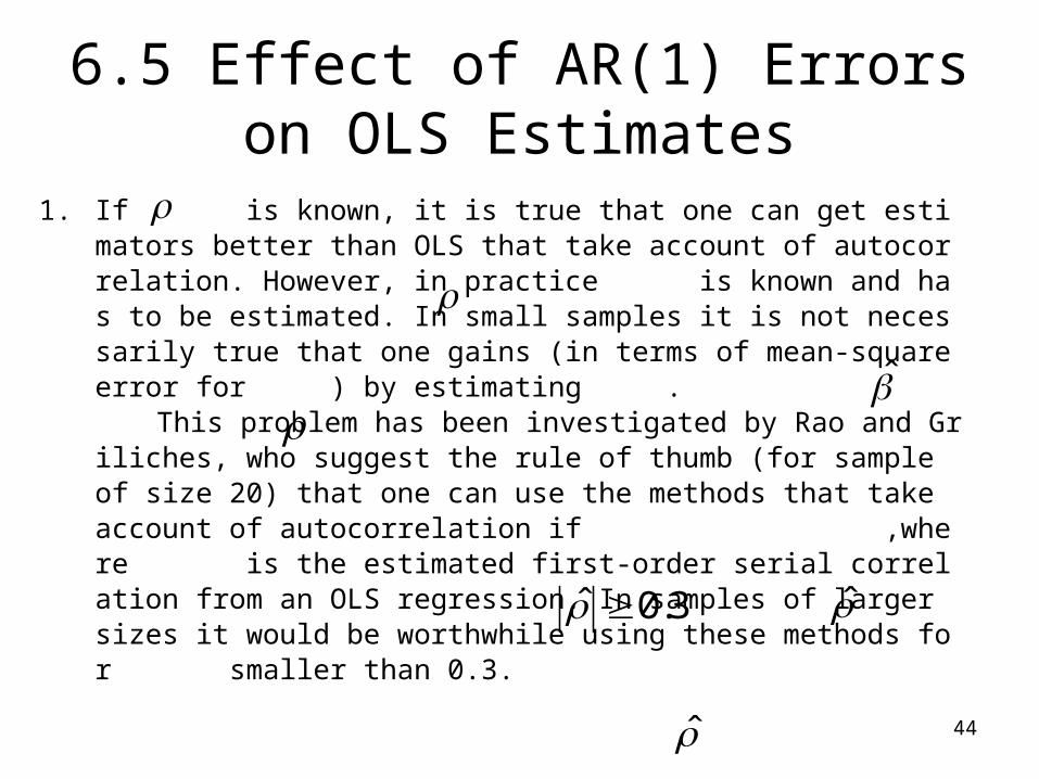
1. If is known, it is true that one can get estimators better than OLS that take account of autocorrelation. However, in practice is known and has to be estimated. In small samples it is not necessarily true that one gains (in terms of mean-square error for ) by estimating .
This problem has been investigated by Rao and Griliches, who suggest the rule of thumb (for sample of size 20) that one can use the methods that take account of autocorrelation if ,where is the estimated first-order serial correlation from an OLS regression. In samples of larger sizes it would be worthwhile using these methods for smaller than 0.3.
3.0ˆ

45
6.5 Effect of AR(1) Errors on OLS Estimates
• 2. The discussion above assumes that the true errors are first-order autoregressive. If they have a more complicated structure (e.g., second-order autoregressive), it might be thought that it would still be better to proceed on the assumption that the errors are first-order autoregressive rather than ignore the problem completely and use the OLS method???
– Engle shows that this is not necessarily true (i.e., sometimes one can be worse off making the assumption of first-order autocorrelation than ignoring the problem completely).

46
6.5 Effect of AR(1) Errors on OLS Estimates
3. In regressions with quarterly (or monthly) data, one might find that the errors exhibit fourth (or twelfth)-order autocorrelation because of not making adequate allowance for seasonal effects. In such case if one looks for only first-order autocorrelation, one might not find any. This does not mean that autocorrelation is not a problem. In this case the appropriate specification for the error term may be for quarterly data and monthly data.
ttt euu 4ttt euu 12
47
6.5 Effect of AR(1) Errors on OLS Estimates
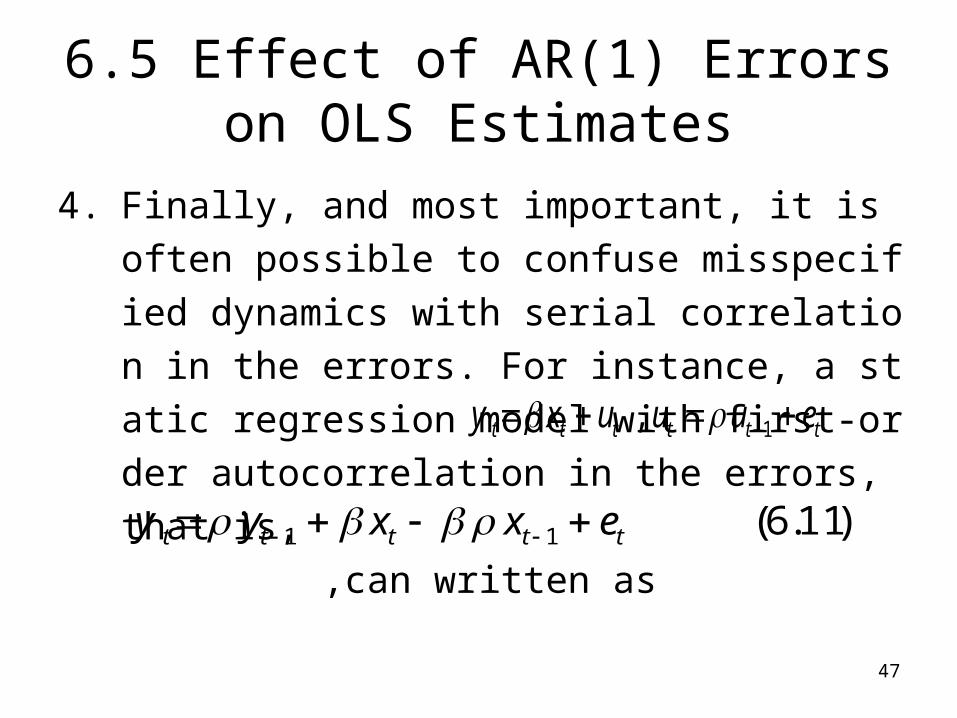
4. Finally, and most important, it is often possible t
o confuse misspecified dynamics with serial corr
elation in the errors. For instance, a static regres
sion model with first-order autocorrelation in the
errors, that is, ,can writte
n astttttt euuuxy 1,
)11.6(11 ttttt exxyy

48
6.5 Effect of AR(1) Errors on OLS Estimates
4. The model is the same as
with the restriction .
We can estimate the model (6.11’) and test this restriction. If it is rejected, clearly it is not valid to estimate (6.11).(the test procedure is described in Section 6.8.)
)'11.6(13211 ttttt exxyy
0321

49
6.5 Effect of AR(1) Errors on OLS Estimates
• The errors would be serially correlated but not b
ecause the errors follow a first-order autoregress
ive process but because the term xt-1 and yt-1 hav
e been omitted.
• Thus is what is meant by “misspecified dynamics.
” Thus significant serial correlation in the estimat
ed residuals does not necessarily imply that we
should estimate a serial correlation model.

50
6.5 Effect of AR(1) Errors on OLS Estimates
• Some further tests are necessary (like the
restriction in the above-
mentioned case).
• In fact, it is always best to start with an equation
like (6.11’) and test this restriction before
applying any test for serial correlation.
0321

51
6.7 Tests for Serial Correlation in Models with Lagged Dependent Variables
• In previous sections we considered explanatory variables that were uncorrelated with the error term
• This will not be the case if we have lagged dependent variables among the explanatory variables and we have serially correlated errors
• There are several situations under which we would be considering lagged dependent variables as explanatory variables
• These could arise through expectations, adjustment lags, and so on.
• Let us consider a simple model

52
6.7 Tests for Serial Correlation in Models with Lagged Dependent Variables
• Let us consider a simple model
• et are independent with mean 0 and variance σ2 and .
• Because ut depends on ut-1 and yt-1 depends on u
t-1, the two variables yt-1 and ut will be correlated.
1,1

53
6.7 Tests for Serial Correlation in Models with Lagged Dependent Variables
An example

54
6.7 Tests for Serial Correlation in Models with Lagged Dependent Variables
Durbin’s h-Test
• Since the DW test is not applicable in these models, Durbin suggests an alternative test, called the h-test.
• This test uses
as a standard normal variable.
)ˆ(ˆ1ˆ
Vn
nh

55
6.7 Tests for Serial Correlation in Models with Lagged Dependent Variables
• Hence is the estimated first-order serial
correlation from the OLS residual, is the
estimated variance of the OLS estimate of α,
and n is the sample size.
• If , the test is not applicable. In this
case Durbin suggests the following test.
)ˆ(ˆ V
1)ˆ(ˆ Vn

56
6.7 Tests for Serial Correlation in Models with Lagged Dependent Variables
Durbin’s Alternative Test• From the OLS estimation of equation(6.12)
compute the residuals .• Then regress
• The test for ρ=0 is carried out by testing the significance of the coefficient of in the latter regression.
tu
tttt xyuu and,,ˆonˆ 11
1ˆ tu

57
6.7 Tests for Serial Correlation in Models with Lagged Dependent Variables
• An equation of demand for food estimated from 50 observations gave the following results (figures in parentheses are standard errors):
where qt=food consumption per capita pt=food price (retail price deflated by the consumer price index) yt=per capita disposable income deflated by the consumer price index

58
6.7 Tests for Serial Correlation in Models with Lagged Dependent Variables
• We have
• Hence Duribin’s h-statistic is
• This is significant at the1%level.• Thus we reject the hypothesis ρ=0, even though the DW
statistic is close to 2 and the estimate from the OLS residuals is
59
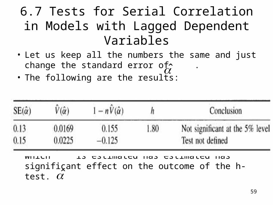
6.7 Tests for Serial Correlation in Models with Lagged Dependent Variables
• Let us keep all the numbers the same and just change the standard error of .
• The following are the results:
• Thus, other things equal, the precision with which is estimated has estimated has significant effect on the outcome of the h-test.

60
6.9 Strategies When the DW Test Statistic is Significant
• The DW test is designed as a test for the hypothesis ρ = 0 if the errors follow a first-order autoregressive process
• However, the test has been found to be robust against other alternatives such as AR(2), MA(1), ARMA(1, 1), and so on.
• Further, and more disturbingly, it catches specification errors like omitted variables that are themselves autocorrelated, and misspecified dynamics (a term that we will explain).
• Thus the strategy to adopt, if the DW test statistic is significant, is not clear.
• We discuss two different strategies:
61
6.9 Strategies When the DW Test Statistic is Significant
• 1. Test whether serial correlation is due to omitted variables.
• 2. Test whether serial correlation is due to misspecified dynamics.

62
6.9 Strategies When the DW Test Statistic is Significant
Autocorrelation Caused by Omitted Variables
• Suppose that the true regression equation is
and instead we estimate
tttt uxxy 2210
)20.6(10 ttt vxy

63
6.9 Strategies When the DW Test Statistic is Significant
• Then since , if xt is autocorre
lated, this will produce autocorrelation in vt.
• However vt is no longer independent of xt.
• This not only are the OLS estimators of β0 a
nd β1 from (6.20) inefficient, they are inconsi
stent as well.
ttt uxv 22

64
6.9 Strategies When the DW Test Statistic is Significant
• Serial correlation due to misspecification dynamics.• In a seminal paper published in 1964, Sargan pointed
out that a significant DW statistic does not necessarily imply that we have a serial correlation problem.
• This point was also emphasized by Henry and Mizon.• The argument goes as follows.• Consider
and et are independent with a common variable σ2.• We can write this model as
)24.6(1 tttttt euuwithuxy
)25.6(11 ttttt exxyy

65
6.9 Strategies When the DW Test Statistic is Significant
• Consider an alternative stable dynamic model:
• Equation (6.25) is the same as equation(6.26) with the restriction

66
6.9 Strategies When the DW Test Statistic is Significant
• A test for ρ=0 is a test for β1=0 (and β3=0).
• But before we test this, what Sargan says is that we should first test the restriction (6.27) and test for ρ=0 only if the hypothesis is not rejected.
• If this hypothesis is rejected, we do not have a serial correlation model and the serial correlation in the errors in (6.24) is due to “misspecified” dynamics, that is the omission of the variable yt-1 and xt-1 from the eq
uation.
0: 3210 H
67
6.9 Strategies When the DW Test Statistic is Significant
• If the DW test statistic is significant, a proper approach is to test the restriction(6.27) to make sure that what we have is a serial correlation model before we undertake any autoregressive transformation of the variables.
• In fact, Sargan suggests starting with the general model (6.26) and testing the restriction (6.27) first, before attempting any test for serial correlation.

68
6.9 Strategies When the DW Test Statistic is Significant
Illustrative Example
• Consider the data in Table 3.11 and the estimation of the production function (4.24).
• In Section 6.4 we presented estimates of the equation assuming that the errors are AR(1).
• This was based on a DW test statistic of 0.86.
• Suppose that we estimate an equation of the form(6.26).
• The results are as follows (all variables in logs; figures in parentheses are standard errors):

69
6.9 Strategies When the DW Test Statistic is Significant
Illustrative Example
• Under the assumption that the errors are AR(1), the residual sum of squares, obtained from the Hildreth-Lu procedure we used in Section 6.4, is RSS1=0.02635

70
6.9 Strategies When the DW Test Statistic is Significant
• Since we have two slope coefficients, we have two restrictions of the form (6.27).
• Note that for the general dynamic model we estimating six parameters (α and five β’s).
• For the serial correlation model we are estimating four parameters (α, two β’s, and ρ).
• We will use the likelihood ratio test (LR)

71
6.9 Strategies When the DW Test Statistic is Significant
and -2logeλhas a χ2 -distribution with d.f. 2(number of restrictions).
• In our example
which is significant at the 1% level.
• Thus the hypothesis if a first-order autocorrelation is rejected.
• Although the DW statistic is significant, this does not mean that the errors are AR(1).
2/
1
0 )( n
RSS
RSS