1 Bezier Curves and Surfaces © Jeff Parker, Nov 2011

1

Bezier Curves and Surfaces

© Jeff Parker, Nov 2011

Outline

We often wish to generate curves and surfaces

To create objects

To create movement

e.g. Genesis Project

To provide transitions

We will look at a number of ways to generate curves

We will focus on various parametric cubics

ReviewWe often wish to generate curves and surfaces

There are a number of (conflicting) goals

Interpolate (include) a set of arbitrary points

Easy and efficient to compute

Smooth

Local Control

Easy to deal with

We may need to compute derivatives

It is hard to get all of these

We will discuss ways to achieve some of these

4

HistoryThe Bezier curves and surfaces were developed twice:

Pierre Bézier, at Renault

Paul de Casteljau, at Citroën

Used to bend sheet metal or wood to achieve a smooth shape

Background: Interpolation

Given a set of n points (xi, yi) we may be able to define a polynomial that goes through each point.

Solution: Lagrange Polynomial

Assumes no two points with the same x but different y

Thus cannot draw circle

Interpolate set of arbitrary points


Smooth

Local Control

6

Runge Phenomena

Try to approximate the red curve with polynomials

Interpolate (hit curve) at evenly spaced x values

Runge Phenomena

Interpolate at evenly spaced pointsDifficult to get local control with high order polynomials



Smooth

Local Control

Runge Phenomena

To avoid this

We don't always interpolate

We break curve into small polynomial pieces



Smooth

Local Control

9

Terminology

Interpolation vs. Approximation

Functions

Three main ways to define a curve

Function: y = x3 + 3x

A function must be single valued

Cannot draw vertical line or circles with function

Implicit function: x2 + y2 + xy= 25

In general case, can't find all points that satisfy

Parametric Function: (x, y) = (5 cos(t), 5 sin(t))

What we will use tonight

Parametric Functions

We will be exploring Parametric Curves

Parametric Surfaces are similar

€

(x, y)= (cosθ ,sinθ )

(x, y, z) = ( f1(u), f2 (u), f3(u))

(x, y, z) = ( f1(u,v), f2(u,v), f3(u,v))

Natural parameterizationMoves with curve length

Sample Surface

Parametric map the unit square to the sphere

€

(x, y, z) = ( f1(u,v), f2(u,v), f3(u,v))

x(θ ,ϕ ) = r cosθ sinϕ

y(θ ,ϕ ) = r sinθ sinϕ

z(θ ,ϕ ) = r cosϕ

Linear Bezier Curve

We wrote line segments as weighted sum of endpoints

This is the convex sum of the two end points

The curves below are defined on [0..1], sum to 1

Blending Functions

Linear Bezier Curve

In the expression, the terms p0 and p1 are vectors, and their weighted sum is a vector

This is a powerful technique, and we will use it all night

Blending Functions

Piece these together

Piece together a curve that connects a set of points

p1

p2

p3

p4

p0


Piece together a curve that connects a set of points

p1

p2

p3

p4

p0


Create series of equations

p1

p2

p0

p3

p4p1

p2

p3

p4

€

(x, y) =

0 ≤ t <1, (1− t)p0 + tp1

1≤ t < 2, (2 − t)p1 +(t −1)p2

2 ≤ t < 3, (3− t)p1 +(t − 2)p2

3 ≤ t < 4, (4 − t)p1 +(t − 3)p2

4 ≤ t < 5, (5 − t)p1 +(t − 4)p2

⎧

⎨

⎪ ⎪ ⎪

⎩

⎪ ⎪ ⎪

⎫

⎬

⎪ ⎪ ⎪

⎭

⎪ ⎪ ⎪

p0

Blending Functions



p1

p2

p0

p3

p4p1

p2

p3

p4

p0



Smooth

Local ControlBlending Functions



p1

p2

p0

p3

p4p1

p2

p3

p4

p0

T Interpolate set of arbitrary points

T Easy and efficient to compute

F Smooth – Nope - sharp "corners"

T Local ControlBlending Functions



p1

p2

p0

p3

p4p1

p2

p3

p4

p0

What do we want from the blending functions?

Active Blending Functions should sum to 1

Nice to have all non-negative termsBlending Functions

Terminology

Not continuous at break

Not differentiable at corner

Next: C(1) vs G(1)

Geometric Continuity

23

Cubics

We will focus on Cubic curves

That is, curves with cubic blending functions

Reasons

These allow C(1) and even C(2) continuity

Allow minimum-curvature interpolants to a set of points

Can define position and curvature at two ends

Cubic Polynomials are in the sweet spot:

Smooth, and easy to compute

Implemented with 4x4 matrices, just like rest of OpenGL

24

Bezier Animation

http://zonalandeducation.com/mmts/curveFitting/bezierCurves/bca2/Bezier1Animation2.html

25

Note rate of movement

26

Bezier Curve

We will look at Bezier Curves in some detail tonight

There are different ways to think about them:

All paths lead to the same curves

De Castlejau Algorithm (recursive subdivision)

Bernstein Polynomials

Matrix Form

Cubic equations

All have their uses, and you will see all in practice

27

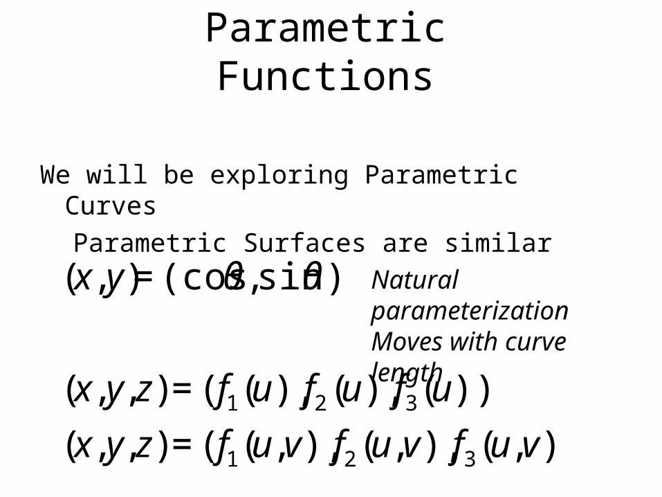
De Casteljau Algorithm

Compute points on the curve without evaluating polynomials

Can use the midpoints, so only need to shift right

28

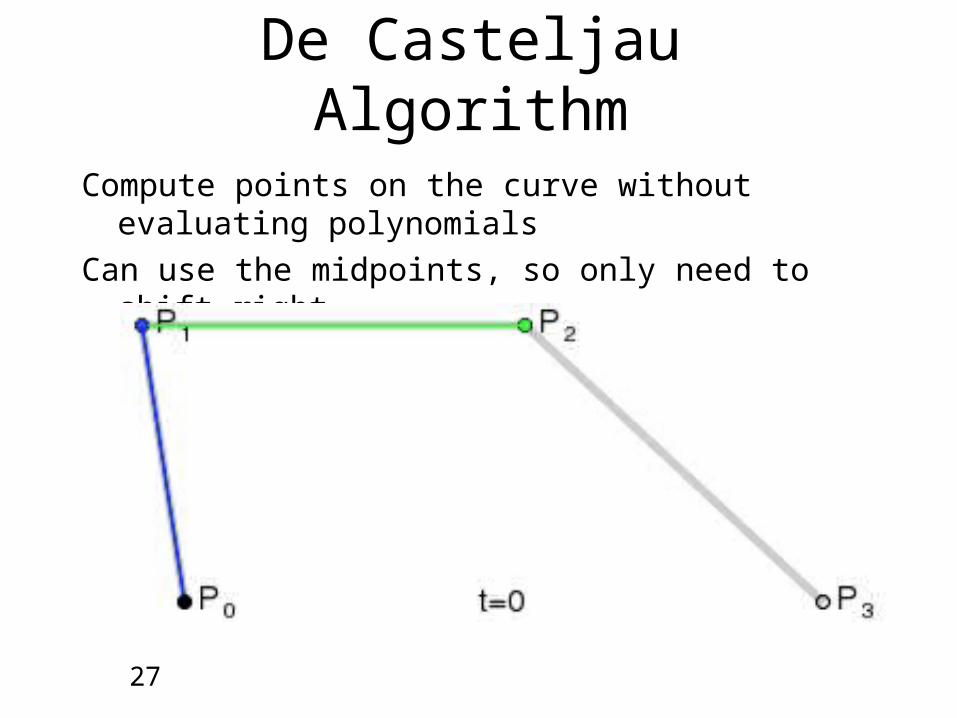
De Casteljau's Method

Compute points on the curve without evaluating polynomials

Can use the midpoints, so only need to shift right

29

De Casteljau's Method

Gives simple recursive method to draw curve

Keep dividing until each subpiece of the curve is almost straight

30

Recursive Drawing Algorithm

We take original four control points

Recursively subdivide, just using adds and shifts

Get two Beziers, with 7 control points

Curve lies inside the convex hull of control points

Continue until the convex hull is one pixel wide

At each step, subcurves

are shorter

are much less wide

Can make this formal

31

Terminology

The Bezier interpolates the first and fourth control point

That is, the curve passes through them

The middle two control points draw the curve towards them

De Casteljau

Let's spell out what this means

Notation differs from figure

€

r0 = (1−u)p0 +u p1

r1 = (1−u)p1 +u p2

r2 = (1−u)p2 +u p3

s0 = (1−u)r0 +ur1s1 = (1−u)r1 +ur2

t0 = (1−u)s0 +us1

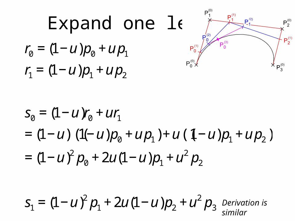
Expand one level

€

r0 = (1−u)p0 +u p1

r1 = (1−u)p1 +u p2

s0 = (1−u)r0 +ur1= (1−u)((1−u)p0 +u p1)+u ((1−u)p1 +u p2 )

= (1−u)2 p0 + 2u(1−u)p1 +u2 p2

s1 = (1−u)2 p1 + 2u(1−u)p2 +u2 p3Derivation is similar

Find third level

€

s0 = (1−u)2 p0 + 2u(1−u)p1 +u2 p2

s1 = (1−u)2 p1 + 2u(1−u)p2 +u2 p3

t0 = (1−u)s0 +us1

= (1−u)3 p0 + 3u(1−u)2 p1 + 3u2(1−u)p2 +u3 p3

35

Bezier Curve

There are different ways to think about them:



Matrix Form

Cubic equations


36


We write a Bezier as the weighted sum of control points

The control points are multiplied by Bernstein polynomials

Convex sum of polynomials with values in [0..1] that sum to 1

Each polynomial pulls curve towards it's control point

What does it mean?We use these blending functions to decide the amount of

contribution from each control point.

Note that the terms add up to one

38 E. Angel and D. Shreiner: Interactive Computer Graphics 6E © Addison-Wesley 2012

Why Polynomials?

Easy to evaluate

Continuous and differentiable everywhere

Must worry about continuity at join points including continuity of derivatives

p(u)

q(u)

join point p(1) = q(0)but p’(1) q’(0)

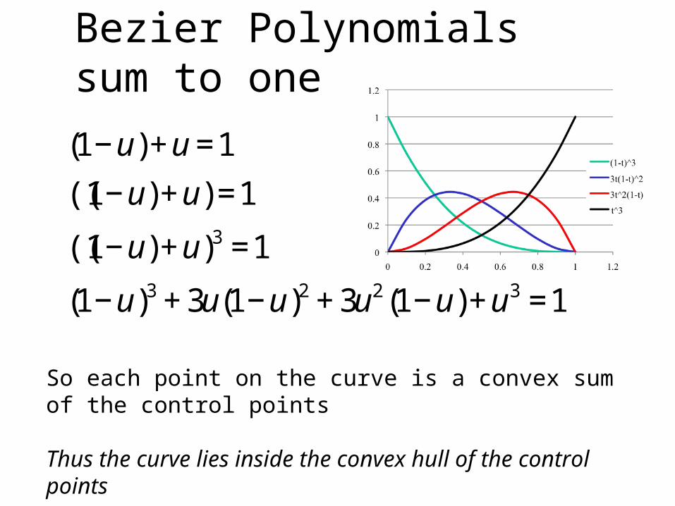
Bezier Polynomials sum to one

€

(1−u)+u =1

((1−u)+u) =1

((1−u)+u)3 =1

(1−u)3 + 3u(1−u)2 + 3u2 (1−u)+u3 =1

So each point on the curve is a convex sum of the control points

Thus the curve lies inside the convex hull of the control points

40

Convex Hull

Check that the curve remains inside the convex hull of the control points in our examples

Also obvious from De Casteljau's Algorithm

41

Bezier Curve

All paths lead to the same point



Matrix Form

Cubic equations


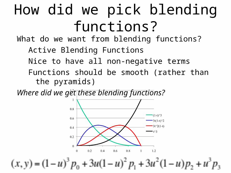
How did we pick blending functions?What do we want from blending functions?

Active Blending Functions

Nice to have all non-negative terms

Functions should be smooth (rather than the pyramids)

Where did we get these blending functions?

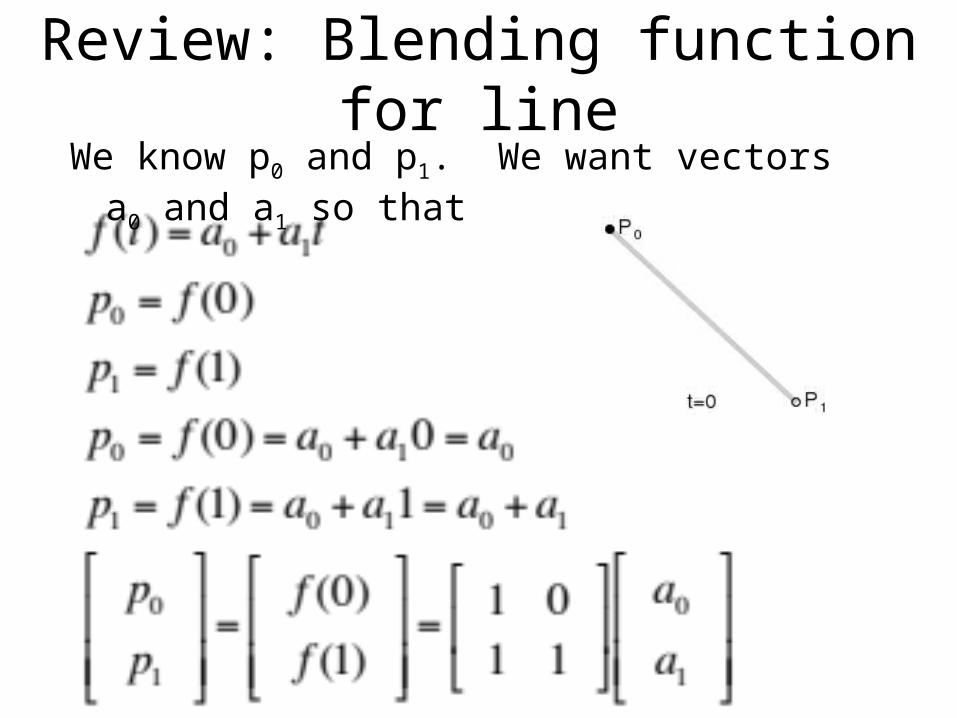
Review: Blending function for lineWe know p0 and p1. We want vectors a0 and a1 so that

Blending function for the lineWe could solve this by hand: a0 = p0, etc.

But let's evolve a general method

Both p and a are vectors

We know p, wish to find aTo solve for p, can invert the Constraint Matrix, C

to find the Blending Matrix, B

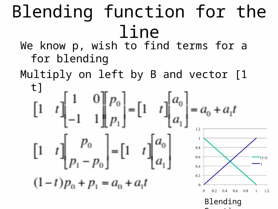
Blending function for the lineWe know p, wish to find terms for a for blending

Multiply on left by B and vector [1 t]

Blending Functions

Blending functions for BezierKnow p0, p1, p2, and p3, want vectors a0, a1, a2, and a3

so that our curve has the form

What do we know?

We know that f(t) interpolates p0 and p3 at t=0 and t=1

Constraint Matrix for BezierWe also know that the slope at the ends is 3(p1-p0)

Compute slope:

Evaluate at t=0 and t=1

€

f '(t) = a1 + 2a2t + 3a3t2

f '(0) = a1

f '(1) = a1 + 2a2 + 3a3

Constraint Matrix for BezierNow we have a constraint matrix C: find it’s inverse B

€

BC =

1 0 0 0

−3 3 0 0

3 −6 3 0

−1 3 −3 1

⎡

⎣

⎢ ⎢ ⎢ ⎢

⎤

⎦

⎥ ⎥ ⎥ ⎥

1 0 0 0

11

30 0

12

3

1

30

1 1 1 1

⎡

⎣

⎢ ⎢ ⎢ ⎢ ⎢

⎤

⎦

⎥ ⎥ ⎥ ⎥ ⎥

=

1 0 0 0

0 1 0 0

0 0 1 0

0 0 0 1

⎡

⎣

⎢ ⎢ ⎢ ⎢

⎤

⎦

⎥ ⎥ ⎥ ⎥

Apply Constraint MatrixApply the vector [1 u u2 u3] to matrix B

€

Bp = a

1 u u2 u3[ ]

1 0 0 0

−3 3 0 0

3 −6 3 0

−1 3 −3 1

⎡

⎣

⎢ ⎢ ⎢ ⎢

⎤

⎦

⎥ ⎥ ⎥ ⎥

p0

p1

p2

p3

⎡

⎣

⎢ ⎢ ⎢ ⎢

⎤

⎦

⎥ ⎥ ⎥ ⎥

= 1 u u2 u3[ ]

a0

a1

a2

a3

⎡

⎣

⎢ ⎢ ⎢ ⎢

⎤

⎦

⎥ ⎥ ⎥ ⎥

(1−u)3 3u(u −1)2 3u2(u −1) u3[ ]

p0

p1

p2

p3

⎡

⎣

⎢ ⎢ ⎢ ⎢

⎤

⎦

⎥ ⎥ ⎥ ⎥

= a0 + a1u + a2u2 + a3u

3

(1−u)3 p0 + 3u(1−u)2 p1 + 3u2(1−u)p2 +u3 p3 = a0 + a1u + a2u2 + a3u

3

51

Bezier Curve

All paths lead to the same point



Matrix Form

Cubic equations


Derive the values ai

Another way to look at this:

€

1 u u2 u3[ ]

1 0 0 0

−3 3 0 0

3 −6 3 0

−1 3 −3 1

⎡

⎣

⎢ ⎢ ⎢ ⎢

⎤

⎦

⎥ ⎥ ⎥ ⎥

p0

p1

p2

p3

⎡

⎣

⎢ ⎢ ⎢ ⎢

⎤

⎦

⎥ ⎥ ⎥ ⎥

= 1 u u2 u3[ ]

a0

a1

a2

a3

⎡

⎣

⎢ ⎢ ⎢ ⎢

⎤

⎦

⎥ ⎥ ⎥ ⎥

1 u u2 u3[ ]

p0

3(p1 − p0 )

3( p0 − 2 p1 − p2 )

p3 − 3p2 + 3p1 − p0

⎡

⎣

⎢ ⎢ ⎢ ⎢

⎤

⎦

⎥ ⎥ ⎥ ⎥

= a0 +ua1 +u2a2 +u3a3

p0 + 3u(p1 − p0 )+ 3u2( p0 − 2 p1 − p2 )+u3( p3 − 3p2 + 3p1 − p0 )


NURBS

Nonuniform Rational B-Spline curves and surfaces add a fourth variable w to x,y,z

Can interpret as weight to give more importance to some control data

Can also interpret as moving to homogeneous coordinate

Requires a perspective division

NURBS act correctly for perspective viewing

Quadrics are a special case of NURBS

NURBS

Non-Uniform Rational B-Splines

Note that Rational is usually a restriction

Rational numbers vs all real numbers.

Here it is an extension: Projective Geometry

Example: we wish to draw a unit circle

No exact match with Cubic Beziers – can get close

However, if we use projective space…

€

(0,1,1), (1,0,0), (0,−1,1)

€

p0 = (0,1,1), p1 = (1,0,0), p2 = (0,−1,1)

(x, y, z) = (0,1,1)(1−u)2 + 2(1,0,0)u(1−u)+ (0,−1,1)u2

(x, y, z) = (2u(1−u), (1−u)2 −u2, (1−u)2 +u2 )

North and south pole and point at (Eastern) infinity

We only need a quadratic Bezier for 3 points

Quadratic Bezier

€

(x, y, z) = (2u(1−u), (1−u)2 −u2, (1−u)2 +u2 )

(x, y, z) =2u(1−u)

(1−u)2 +u2,(1−u)2 −u2

(1−u)2 +u2,1

⎛

⎝ ⎜

⎞

⎠ ⎟

x2 + y2 =(2u(1−u))2 +((1−u)2 −u2 )2

(1−u)2 +u2[ ]

2

=4u2 (1−u)2 +(1−u)4 − 2u2 (1−u)2 +u4

(1−u)2 +u2[ ]

2

=(1−u)4 + 2u2 (1−u)2 +u4

(1−u)2 +u2[ ]

2 =1

But are these points on the unit circle?

x

y

€

(x, y, z) = (0,1,1)(1−u)2 + 2(1,0,0)u(1−u)+ (0,−1,1)u2

=[(1−u)+u][(0,1,1)(1−u)2 + 2(1,0,0)u(1−u)+ (0,−1,1)u2 ]

= (0,1,1)(1−u)3 +(0,1,1)u(1−u)2 +

2(1,0,0)u(1−u)2 + 2(1,0,0)u2 (1−u)+

(0,−1,1)u2(1−u)+ (0,−1,1)u3

= (0,1,1)(1−u)3 +u(1−u)2[(0,1,1)+ 2(1,0,0)]+

u2(1−u)[2(1,0,0)+ (0,−1,1)]+ (0,−1,1)u3

= (0,1,1)(1−u)3 +(2,1,1)u(1−u)2 +(2,−1,1)u2 (1−u)+ (0,−1,1)u3

= (0,1,1)(1−u)3 + 3(2

3,1

3,1

3)u(1−u)2 + 3(

2

3,−1

3,1

3)u2 (1−u)+ (0,−1,1)u3

The control points are weightedThis gives NURBS more degrees of freedom

Degree Elevation

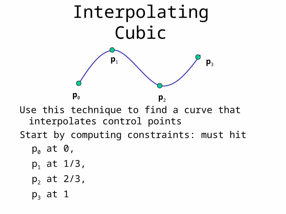
Interpolating Cubic

Use this technique to find a curve that interpolates control points

Start by computing constraints: must hit

p0 at 0,

p1 at 1/3,

p2 at 2/3,

p3 at 1

p0

p1

p2

p3

Interpolating Cubic

Use this technique to find a curve that interpolates control points

Start by computing constraints: must hit

p0 at 0,

p1 at 1/3,

p2 at 2/3,

p3 at 1

p0

p1

p2

p3

€

C =

1 0 0 0

1 1/ 3 1/9 1/27

1 2 / 3 4 /9 8 /27

1 1 1 1

⎡

⎣

⎢ ⎢ ⎢ ⎢

⎤

⎦

⎥ ⎥ ⎥ ⎥


Interpolation MatrixSolving for c we find the interpolation matrix

5.45.135.135.4

5.4185.229

15.495.5

0001

1

AMI

c=MIp

Note that MI does not depend on input data and

can be used for each segment in x, y, and z


Interpolating Multiple Segments

use p = [p0 p1 p2 p3]T use p = [p3 p4 p5 p6]T

Get continuity at join points but notcontinuity of derivatives


Blending FunctionsRewriting the equation for p(u)

p(u)=uTc=uTMIp = b(u)Tp

where b(u) = [b0(u) b1(u) b2(u) b3(u)]T isan array of blending polynomials such thatp(u) = b0(u)p0+ b1(u)p1+ b2(u)p2+ b3(u)p3

b0(u) = -4.5(u-1/3)(u-2/3)(u-1)b1(u) = 13.5u (u-2/3)(u-1)b2(u) = -13.5u (u-1/3)(u-1)b3(u) = 4.5u (u-1/3)(u-2/3)

63 E. Angel and D. Shreiner: Interactive Computer Graphics 6E © Addison-

Wesley 2012

Lagrange Blending FunctionsThese functions are not smooth

Hence the interpolation polynomial is not smooth

Are not limited to [0, 1] – thus not convex

64

Catmull-Rom

We can get a similar effect with Bezier curves

One way of auto-generating the right slopes to a set of interpolated points was introduced by Catmull and Rom

Idea is to use slope between previous and next point as the slope at the current point.

If distance between points is uneven, can overshoot

Cubic Hermite Spline

Sometimes we want to avoid sharp corners

Can define the slope at the endpoints

Hermite Polynomials use a new blending functions to define curve

p(0) p(1)

p’(0) p’(1)

Hermite Polynomial

Hermite Polynomial


AnalysisBezier form has advantages over interpolating form,

derivatives need note be continuous at join points

Can we do better?

Go to higher order Bezier

More work

Derivative continuity still only approximate

Supported by OpenGL

Apply different conditions

Tricky without letting order increase

69

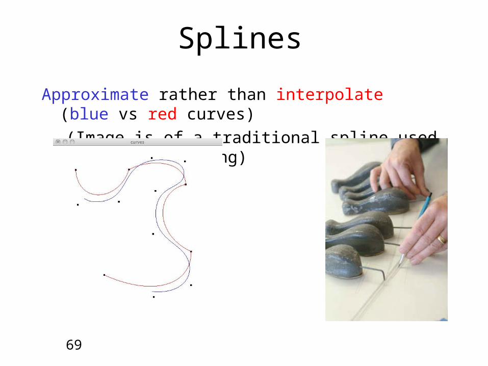
Splines

Approximate rather than interpolate (blue vs red curves)

(Image is of a traditional spline used in boat building)

70E. Angel and D. Shreiner: Interactive Computer

Graphics 6E © Addison-Wesley 2012

B-Splines

Basis splines: use the data at p=[pi-2 pi-1 pi pi-1]T to define curve only between pi-1 and pi

We can apply more continuity conditions to each segment

For cubics, we can have continuity of function, first and second derivatives at join points - C(2)

Cost is 3 times as much work for curves

Add one new point each time rather than three

For surfaces, we do 9 times as much work

71

Cubic B-spline

1331

0363

0303

0141

MS

p(u) = uTMSp = b(u)Tp

E. Angel and D. Shreiner: Interactive Computer Graphics 6E © Addison-Wesley 2012

72

Blending Functions

u

uuuuu

u

u

3

22

32

3

3331

364

)1(

6

1)(b

convex hull property


73

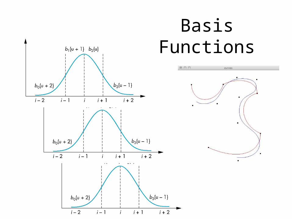
Basis Functions

2

21

11

12

2

0

)1(

)()1(

)2(

0

)(

3

2

1

0

iu

iui

iuiiui

iui

iu

ub

ubub

ub

uBi

In terms of the blending polynomials


Basis Functions

75 E. Angel and D. Shreiner: Interactive Computer Graphics 6E © Addison-

Wesley 2012

B-Spline Patches

vupvbubvup TSS

Tijj

i ji MPM

)()(),(3

0

3

0

defined over only 1/9 of region


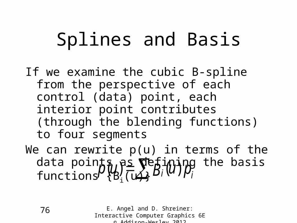
Splines and Basis

If we examine the cubic B-spline from the perspective of each control (data) point, each interior point contributes (through the blending functions) to four segments

We can rewrite p(u) in terms of the data points as defining the basis functions {Bi(u)}

puBup ii )()(

77

Generalizing Splines

We can extend to splines of any degree

Data and conditions do not have to given at equally spaced values (the knots)

Nonuniform and uniform splines

Can have repeated knots

Can force spline to interpolate points

Cox-deBoor recursion gives method of evaluation


78

Beziers in OpenGL

We could evaluate Beziers by hand, given the formulas above.

It is simpler to use Evaluators, provided by OpenGL

Evaluators provide a way to use polynomial or rational polynomial mapping to produce vertices, normals, texture coordinates, and colors. The values produced by an evaluator are sent to further stages of GL processing just as if they had been presented using glVertex, glNormal, glTexCoord, and glColor commands, except that the generated values do not update the current normal, texture coordinates, or color.

All polynomial or rational polynomial splines of any degree (up to the maximum degree supported by the GL implementation) can be described using evaluators. These include almost all splines used in computer graphics: B-splines, Bezier curves, Hermite splines, and so on. (From the man page)

Bezier Curve

void drawCurve() {

int i;

GLfloat pts[4][3];

/* Copy the coordinates from balls to array */

for (i = 0; i < 4; i++) {

pts[i][0] = (GLfloat)cp[i]->x;

pts[i][1] = (GLfloat)wh - (GLfloat)cp[i]->y;

pts[i][2] = (GLfloat)0.0;

}

// Define the evaluator

glMap1f(GL_MAP1_VERTEX_3, 0.0, 1.0, 3, 4, &pts[0][0]);

/* type, u_min, u_max, stride, num points, points */

glEnable(GL_MAP1_VERTEX_3);

setLineColor();

glBegin(GL_LINE_STRIP);

for (i = 0; i <= 30; i++)

/* Evaluate the curve when u = i/30 */

glEvalCoord1f((GLfloat) i/ 30.0);

glEnd();

Teapot

bteapot.c

// vertices.h

GLfloat vertices[306][3]={{1.4 , 0.0 , 2.4}, {1.4 , -0.784 , 2.4},

{0.784 , -1.4 , 2.4}, {0.0 , -1.4 , 2.4}, {1.3375 , 0.0 , 2.53125},

{1.3375 , -0.749 , 2.53125}, {0.749 , -1.3375 , 2.53125}, {0.0 , -1.3375 , 2.53125},

{1.4375 , 0.0 , 2.53125}, {1.4375 , -0.805 , 2.53125}, {0.805 , -1.4375 , 2.53125},

...

// patches.h

int indices[32][4][4]={{1, 2, 3, 4, 5, 6, 7, 8, 9, 10, 11, 12, 13, 14, 15, 16},

{4, 17, 18, 19, 8, 20, 21, 22, 12, 23, 24, 25, 16, 26, 27, 28},

{19, 29, 30, 31, 22, 32, 33, 34, 25, 35, 36, 37, 28, 38, 39, 40},

...

bteapot.c

/* 32 patches each defined by 16 vertices, arranged in a 4 x 4 array */

/* NOTE: numbering scheme for teapot has vertices labeled from 1 to 306 */

/* remnent of the days of FORTRAN */

#include "patches.h"

void display(void)

{

int i, j, k;

glClear(GL_COLOR_BUFFER_BIT | GL_DEPTH_BUFFER_BIT);

glColor3f(1.0, 1.0, 1.0);

glLoadIdentity();

glTranslatef(0.0, 0.0, -10.0);

glRotatef(-35.26, 1.0, 0.0, 0.0);

glRotatef(-45.0, 0.0, 1.0, 0.0);

/* data aligned along z axis, rotate to align with y axis */

glRotatef(-90.0, 1.0,0.0, 0.0);

bteapot.c

for(k=0;k<32;k++)

{

glMap2f(GL_MAP2_VERTEX_3, 0, 1, 3, 4, 0, 1, 12, 4, &data[k][0][0][0]);

for (j = 0; j <= 8; j++)

{


for (i = 0; i <= 30; i++)

glEvalCoord2f((GLfloat)i/30.0, (GLfloat)j/8.0);

glEnd();


for (i = 0; i <= 30; i++)

glEvalCoord2f((GLfloat)j/8.0, (GLfloat)i/30.0);

glEnd();

}

}

glFlush();

}

84

Interactive Websites to try

Bill Casselman's Bezier Applet

http://www.math.ubc.ca/people/faculty/cass/gfx/bezier.html

Wikepedia Animation

http://en.wikipedia.org/wiki/Bezier_curve

Edward A. Zobel's Animation

http://id.mind.net/~zona/mmts/curveFitting/bezierCurves/bezierCurve.html

POV-Ray Cyclopedia Tutorial

http://www.spiritone.com/~english/cyclopedia/bezier.html

Andy Salter's Spline Tutorial

http://www.doc.ic.ac.uk/%7Edfg/AndysSplineTutorial/index.html

Evgeny Demidov's Interactive Tutorial

http://ibiblio.org/e-notes/Splines/Intro.htm

85

Summary

86

SummaryWe often wish to generate curves and surfaces

We would like

Interpolate (include) a set of arbitrary points


Smooth

Local Control…

By splicing together pieces of curves, we can attain many of these.

Modern hardware and language support these curves

Documents

1 Bezier Curves and Surfaces © Jeff Parker, Nov 2011