1 Asynchronous Federated Learning with Differential

arX

iv:1

912.

0790

2v1

[cs

.LG

] 1

7 D

ec 2

019

1

Asynchronous Federated Learning withDifferential Privacy for Edge Intelligence

Yanan Li, Shusen Yang, Xuebin Ren, and Cong Zhao

Abstract—Federated learning has been showing as a promising approach in paving the last mile of artificial intelligence, due to its

great potential of solving the data isolation problem in large scale machine learning. Particularly, with consideration of the heterogeneity

in practical edge computing systems, asynchronous edge-cloud collaboration based federated learning can further improve the

learning efficiency by significantly reducing the straggler effect. Despite no raw data sharing, the open architecture and extensive

collaborations of asynchronous federated learning (AFL) still give some malicious participants great opportunities to infer other parties’

training data, thus leading to serious concerns of privacy. To achieve a rigorous privacy guarantee with high utility, we investigate to

secure asynchronous edge-cloud collaborative federated learning with differential privacy, focusing on the impacts of differential privacy

on model convergence of AFL. Formally, we give the first analysis on the model convergence of AFL under DP and propose a

multi-stage adjustable private algorithm (MAPA) to improve the trade-off between model utility and privacy by dynamically adjusting

both the noise scale and the learning rate. Through extensive simulations and real-world experiments with an edge-could testbed, we

demonstrate that MAPA significantly improves both the model accuracy and convergence speed with sufficient privacy guarantee.

Index Terms—Distributed machine learning, Federated learning, Asynchronous learning, Differential privacy, Convergence.

1 INTRODUCTION

MACHINE learning (ML), especially the deep learning,can sufficiently release the great utility in big data,

and has achieved great success in various application do-mains, such as natural language processing [1], [2], objectiondetection [3], [4], and face recognition [5], [6]. However,with the increasing public awareness of privacy, more andmore people are reluctant to provide their own data [7]–[9]. At the same time, large companies or organizationsalso begin to realize that the curated data is their coralassets with abundant business value [10], [11]. Under such acircumstance, a series of ever-strictest data regulations likeGDPR [12] have also been legislated to forbid the arbitrarydata usage without user permission as well as any kindof cross-organization data sharing. The increasing concernof data privacy has been causing serious data isolationproblems across domains, which poses great challenges invarious ML applications.

Aiming to realize distributed ML with privacy protec-tion, federated learning [13], [14] (FL) has demonstrated thegreat potential of conducting large scale ML on enormoususers’ edge devices or distributed network edge serversvia parameter based collaborations, which avoid the directraw data sharing. For example, Google embedded FL intoAndroid smartphones to improve mobile keyboard predic-tion without collecting users’ input [15], which may includesensitive data like the credit numbers and home addresses,etc. Besides, with the great ability of bridging up the AIservices of different online platforms, FL has been seen asa promising facility for a series of innovative AI businessmodels, such as health-care [16], insurance [17] and fraud

Y. Li and S. Yang are with School of Mathematics and Statistics, Xi’anJiaotong University, Shaanxi 710049, P.R. China; X. Ren is with Schoolof Computer Science and Technology, Xi’an Jiaotong University, Shaanxi710049, P.R. China; C. Zhao is with the Department of Computing, ImperialCollege London, London SW7 2AZ, UK.

Fig. 1. Application scenarios of asynchronous federated learning.

detection [18]. Compared with distributed ML in the Cloudserver, FL relies on a large number of heterogeneous edgedevices/servers, which would have heterogeneous trainingprogress and cause severe delays for the collaborative FLtraining. Therefore, asynchronous method has long beenleveraged in deep learning to improve the learning effi-ciency via reducing the straggler effect [19]–[23]. In thispaper, we focus on asynchronous federated learning (AFL)in the context of edge-cloud system with heterogeneousdelays [24], as shown in Fig. 1.

The basic privacy protection of FL benefits from thefact that all raw data are stored locally and close to theirproviders. However, this is far from sufficient privacy pro-tection. On the one hand, it has been proved that variousattacks [25]–[27] can be launched against either ML gradi-ents or trained models to extract the private informationof data providers. For example, both the membership in-ference attack [27] and model inversion attack [25] havebeen validated to be able to infer the individual data or

http://arxiv.org/abs/1912.07902v1

2

recover part of training data, as shown in Fig. 1. On theother hand, the open architecture and extensive collabora-tions make FL systems rather vulnerable to these privacyattacks. Particularly, considering the extensive attacks inother distributed systems like cyber-physical systems, it isnot hard to imagine that both the participating edges or theCloud server in the AFL may act as the honest but curiousadversaries to silently infer the private information from theintermediate gradients or the trained models.

To further secure FL, encryption based approaches likesecure multi-party computation [8] and homomorphic en-cryption [28] have been proved to be highly effective andable to provide strong security guarantee. However, theseapproaches are based on complicated computation proto-cols, leading to potentially unaffordable overheads for edgedevices such as mobile phones. Alternatively, by addingproper noises, differential privacy (DP [29]) can preventprivacy leakage from both the gradients and the trainedmodels with high efficiency, therefore, has also attractedgreat attentions in machine learning as well as FL [7], [9],[24], [30]–[32].

Nonetheless, most of the existing work on DP withFL consider synchronous FL, which are different from ourresearch on DP for general edge-cloud collaboration basedAFL. Specifically, we study the analytical convergence ofAFL under DP in this paper. Based on the analytical results,we propose the multi-stage adjustable private algorithm(MAPA), a gradient-adaptive privacy-preserving algorithmfor AFL to provide both high model utility under the rigor-ous guarantee of differential privacy. Our contributions arelisted as follows.

1) We theoretically analyze the error bound of AFLwith considering DP. In particular, the average errorbound after T iterations under expectation is dom-

inated by O(

1√T

(σ√b+ ∆S

ε

)

+τ2max log T

T

)

(Theo-

rem 2), which extends the result O(σ/√bT ) for

general ML and the result O(

σ√bT

+τ2max log T

T

)

for

AFL without considering DP.2) We prove that the gradient norm can converge at

the rate O(1/T ) to a ball under expectation, theradius of which is determined by the variancesof random sampling and added noise. We furtherpropose MAPA to adjust both the DP noise scalesand learning rates dynamically to achieve a tighterand faster model convergence without complex pa-rameters tuning.

3) We conducted extensive simulations and real-worldedge-cloud testbed experiments1 to thoroughlyevaluate MAPA’s performance in terms of modelutility, training speed, and robustness. During ourevaluation, three types of ML models includinglogistic regression (LR), support vector machine(SVM), and convolutional neural network (CNN)were adopted. Experimental results demonstratethat, for AFL under DP, MAPA manages to guar-antee high model utilities. Specifically, for CNNtraining on our real-world testbed, MAPA manages

1. Source code available at https://github.com/IoTDATALab/MAPA.

to achieve nearly the same model accuracy as thatof centralized training without considering DP.

The rest of this paper is structured as follows. Section2 reviews the related work. Section 3 presents the systemmodels of AFL and gives the problem definition. Section 4introduces our privacy model of differential privacy. Section5 describes a baseline algorithm with DP and derives the an-alytical results on its model convergence. Section 6 proposesthe main algorithms in details and Section 7 demonstratesthe extensive experimental results. Lastly, we conclude thispaper in Section 8.

2 RELATED WORK

Machine learning privacy has gradually become the crucialobstacle for the data-hungry ML applications [7]–[9], [24],[30]–[35]. In spite of restricting raw data sharing, FL, asa new paradigm of ML, still suffers from various indirectprivacy attacks existed in ML, such as membership inferenceattack [27] and model inversion attack [25]. To enhancethe privacy guarantee of FL, many different techniqueshave been leveraged to prevent the indirect leakage, suchas secure multiparty computation [8], homomorphic en-cryption [28], secret sharing [33], and differential privacy[30]. However, most of the schemes like secure multipartycomputation, homomorphic encryption, secret sharing relyon complicated encryption protocols and would incur unaf-fordable overheads for edge devices.

Due to the high effectiveness and efficiency, DP has beenextensively applied in general machine learning [30], [36]–[39] as well as federated learning algorithms [7], [9], [31],[32], [40], [41]. When implementing DP in machine learning,Laplace or Gaussian mechanism is usually adopted to addproperly calibrated noise according to the global sensitivityof gradient’s norm, which, however, is difficult to estimatein many machine learning models, especially the deep learn-ing.

For centralized machine learning, [42] proposes to lever-age the reparametrization trick from [43] to estimate theoptimal global sensitivity. Also, [44] presents the idea ofconducting a projection after each gradient step to boundthe global sensitivity. However, both [42] and [44] incurgreat computational overhead in the optimization or pro-jection. Recently, with a slight sacrifice of training utility,[30] introduces to clip the gradient to bound the gradientsensitivity and propose the momentum account mechanismto accurately track the privacy budget. However, it remainsunclear how to set the optimal clipping bound for achievinga good utility.

For Federated learning, the similar idea of bounding theglobal sensitivity is adopted. For example, [7] samples a sub-set of gradients and truncate the gradients in the subset, thusreducing the communication cost as well as the varianceof the noise. With the similar goal, [32] designs Binomialmechanism, a discrete version of Gaussian mechanism, totransmit noisy and discretized gradient. Besides the sample-level DP considered in the above research, [31] proposes toprovide client-level DP to hide the existence of participantedge servers and adopts the moment account techniqueproposed in [30]. Furthermore, [9] considers both sample-level and client-level for FedSGD and FedAvg respectively.

3

In all these works, to reduce the noise, the gradientis clipped by a fixed estimation, which would still incuran overdose of noise in the subsequent iterations sincethe gradient variance will generally decrease as the modelconverges. Besides, empirical clipping cannot be easily ap-plicable to general ML algorithms. Recently, [41] introducesa new adaptive clipping technique for SFL with user-levelDP, which can realize adaptive parameter tuning. However,no theoretical analysis on model convergence is given,which means the clipped gradient may not guarantee theconvergence or obtain any model utility.

In this paper, we propose an adaptive gradient clippingalgorithm by analyzing the impact of DP on AFL modelconvergence, which ensures that the differentially privateAFL model can converge to a high utility model withoutcomplicated parameters tuning.

3 SYSTEM MODELS AND PROBLEM STATEMENT

In this section, we introduce the system model of an asyn-chronous federated learning.

3.1 Stochastic Optimization based Machine Learning

Generally, the trained learning model can be defined as thefollowing stochastic optimization problem

minx∈RN

f(x) := Eξ∈PF (x; ξ), (1)

where ξ is a random sample whose probability distributionP is supported on the setD ⊆ R

N and x is the global modelweight. F (·, ξ) is convex differentiable for each ξ ∈ D, sothe expectation function f(x) is also convex differentiableand ∇f(x) = Eξ[∇F (x, ξ)].

Assumption 1. Assumptions for stochastic optimization.

• (Unbiased Gradient) The stochastic gradient ∇F (x, ξ) isbounded and unbiased, that is to say,

‖∇F (x, ξ)‖ ≤ G, ∇f(x) = Eξ∇F (x, ξ). (2)

• (Bounded Variance) The variance of stochastic gradient isbounded, that is, ∀x ∈ R

N ,

Eξ[‖∇xF (x, ξ)−∇f(x)‖2∗] ≤ σ2. (3)

• (Lipschitz Gradient) The gradient function ∇F (·) is Lip-schitzian, that is to say, ∀x, y ∈ R

N ,

‖∇xF (x, ξ)−∇xF (y, ξ)‖∗ ≤ L‖x− y‖. (4)

It should be noted that under these assumptions,∇f(x)is Lipschitz continuous with the same constant L [45].

3.2 Asynchronous Update based Federated Learning

As shown in Fig. 2, we consider an asynchronous updatebased federated learning, in which, a common machinelearning model is trained via iterative collaborations amonga Cloud server and K edge servers. In particular, the Cloudserver maintains a global model xt at the t-th iteration whileeach edge server maintains a delayed local model xt−τ(t,k),where τ(t, k) ≥ 0 means the staleness of the k-th edge servercompared to the current model xt. The edge servers and the

Cloud server perform the following collaborations duringthe learning process.

• At first, models in the Cloud server and edge serversare initialized as the same x1 and the number ofiterations t increased by one once the global modelin the Cloud server is updated.

• Then, the k-th edge server at t-th iteration com-putes the gradient gt−τ(t,k) on a data batch Bkwith b random samples ξt,ibi=1 of its local datasetDk and sends gt−τ(t,k) to the Cloud server, wheregt−τ(t,k) =

1b

∑

ξi∈B∇F (xt−τ(t,k), ξi).• The Cloud server each time picks up a gradient

gt−τ(t) from the buffer gt−τ(t,k)Kk=1 with the ”first-in first-out” principle to update the global modelfrom xt to xt+1, which is immediately returned tothe corresponding k(t)-th edge server for next localgradient computation.

• This collaboration continues until the predefinednumber of iterations T is satisfied.

The AFL architecture in our considered scenario is openand scalable. That means any new edge servers obey theprotocols can join in the system and begins training bydownloading the trained model from the Cloud server.Then, like the existing edge servers, they can compute thegradient independently and just communicates with theCloud server.

Assumption 2. Assumptions for asynchronous update.

• (Independence) All random samples in ξt,i are indepen-dent to each other, where t = 1, · · · , T, i = 1, · · · b;

• (Bounded delay) All delay variables τ(t, k) are bounded:maxt,k τ(t, k) ≤ τmax, where k = 1, · · · ,K .

The independence assumption strictly holds if all edgeservers selects samples with replacement. The assumptionon bounded delay is commonly used in the asynchronousalgorithms [19], [20], [46], [47]. Intuitively, the delay (orstaleness) should not be too large to ensure the convergence.

3.3 Adversary Model

We focus on data privacy in machine learning and considera practical federated learning scenario that both the Cloudserver and distributed edge servers may be honest-but-curious, which means they will honestly follow the protocolwithout modifying the interactive data but may be curiousabout and infer the private information of other participantedge servers. In particular, we assume that the untrustwor-thy Cloud server can infer the private information from thereceived gradient and some adversarial edge servers mayinfer the information through the received global models.This adversary model is quite practical in federated learningas all participating entities in the system may locate far fromeach other but have the knowledge of the training modeland related protocols [26], [48].

Therefore, in this paper, we aim to design an effectiveprivacy-preserving mechanism for an asynchronous updatebased federated learning. For convenience, main notationsare listed in Table 1.

4

TABLE 1Notations

∇F (x, ξ) gradient computed on a sample ξ∇f(x) unbiased estimation of ∇F (x, ξ)

g(x) average gradient 1/b∑b

i=1 ∇F (x, ξi)g(x) noisy gradient g = g(x) + ηb, η mini-batch size, random noise vectorL, σ2 Lipschitz smooth constant, variance of ∇F (x, ξ)

τmax,∆S maximal delay, global sensitivity in DPεk privacy level for the k-th edge server

R,G space radius R and upper bound of ‖∇F (x, ξ)‖T,K number of total iterations and edge servers∆0 maximal noise variance maxk=1,··· ,M2∆S2/ε2

k

∆b notation denotes ∆b = σ2/b+∆0

γt the learning rate used in the t-th iteration

4 DIFFERENTIAL PRIVACY

DP is defined on the conception of the adjacent dataset [49].By adding random noise, DP guarantees the probability ofoutputting any same result on two adjacent datasets is lessthan a given constant. In this article, we aim to guaranteethe impact of any single sample will not affect the mini-batch stochastic gradient too much by injecting noise from acertain distribution.

Definition 1. (Differential Privacy) A randomized algorithm Ais (ε, δ)-DP if for two datasets D, D′ differing one sample, andfor all ω, in the output space Ω of A, it satisfies that

Pr[A(D) = ω] ≤ eε Pr[A(D′) = ω] + δ. (5)

The probability is flipped over the randomness ofA. Theadditive term δ allows for breaching ε-DP with the proba-bility δ. Here ε denotes the protection level and smaller εmeans higher privacy preservation level.

DP can be usually achieved by adding a noise vector η[50], [51] to the gradient. The norm of the noise vector η hasthe density function as

h(η;λ) = 1/(2λ) exp(−‖η‖/λ)where, λ is the scale parameter decided by the privacy levelε and the global sensitivity ∆S as λ = ∆S/ε.

Definition 2. (Global Sensitivity ∆S) For any two mini-batchesB and B′, which differ in exactly one sample, the global sensitivity∆S of gradients is defined as

∆S = maxt,B,B′

‖gt(B)− gt(B′)‖.

5 BASELINE ALGORITHM WITH DIFFERENTIAL

PRIVACY

Before presenting our adaptive-clipping algorithm MAPAfor AFL, we first propose a comparable straightforward DPalgorithm for AFL based on the system model and analyzeits convergence.

5.1 AUDP: an Asynchronous Update Federated Learn-

ing algorithm with Differential Privacy

According to the asynchronous federated learning frame-work listed in Section 3.2, we propose a baseline scheme,called Asynchronous Update with Differential Privacy(AUDP), to fulfill the privately asynchronous federated

Fig. 2. An secure asynchronous federated learning framework.

learning, in which all edge servers inject DP noise to perturbthe gradients before uploading to the Cloud. The detailedcollaborations among edge servers and the Cloud server arelisted as follows.

On each edge server’s side (e.g., the k-th edge server),the following steps are performed independently.

1) Send the privacy budget εk to the Cloud server;2) Pull down the current global model xt from the

Cloud server;3) Compute a noisy gradient gt ← gt + ηt by adding

a random noise ηt drawn from the distribution withthe density function

h(η, εk) =εk

2∆Sexp

(

−εk‖η‖∆S

)

; (6)

4) Push gt back to the Cloud server;

Meanwhile, the Cloud server performs the following steps.

1) At the current t-th iteration, pick a stale gradientgt−τ(t,k) delayed by τ(t, k) iterations provided bythe k(t)-the edge server from the buffers, whereτ(t, k)2 ranging from 0 to the maximum delay τmax;

2) Update the current global model xt using gradientdescent method

xt+1 = xt − γtgt−τ(t),

where, γt is the learning rate at t-th iteration andhas relation to εk;

3) Send xt+1 to the k(t)-th edge server;

The basic workflow of AUDP is also shown in Fig. 2.For example, based on the global model x2, edge server 3computes a local gradient g2 and sends a noisy gradient g2to the buffer in the Cloud server. When g2 is picked up,the original model x2 has been updated by 6 updates andbecomes x8 at now. So, the Cloud server has to use the stalegradient g2 to update x8 and sends the newly updated x9

back to edge server 3 for the next local computing. Otheredge servers perform a similar process without waiting forothers.

Now, we prove that the t-th iteration of AUDP satisfiesεk(t)-DP.

Theorem 1. Assume the upper bound of the gradients is G, i.e.,‖∇F (x, ξ)‖ ≤ G for all x and ξ. If the global sensitivity is set

2. For simplicity, τ(t, k) is written as τ(t) later.

5

as ∆S = 2G/b and the noise is drawn from the distribution inEq. (6), then the t-th iteration of AUDP satisfies εk(t)-DP.

Proof. For any two mini-batches differing one sample de-noted as ξb ∈ B and ξ′b ∈ B′ without loss of the generality,because

maxt,B,B′

‖gt(B)− gt(B′)‖

= maxt,B,B′

‖∇F (x, ξb)−∇F (x, ξ′b)‖/b ≤ 2G/b,

so the global sensitivity ∆S = 2G/b. For any possibly noisygradient ν, we have

Prgt(B) + η = νPrgt(B′) + η = ν =

exp(−εk(t)‖ν − gt(B)‖/∆S)

exp(−εk(t)‖ν − gt(B′)‖/∆S)

≤ exp

(εk(t)‖gt(B)− gt(B′)‖

∆S

)

≤ exp(εk).

So, the t-th iteration of AUDP satisfies εk(t)-DP.

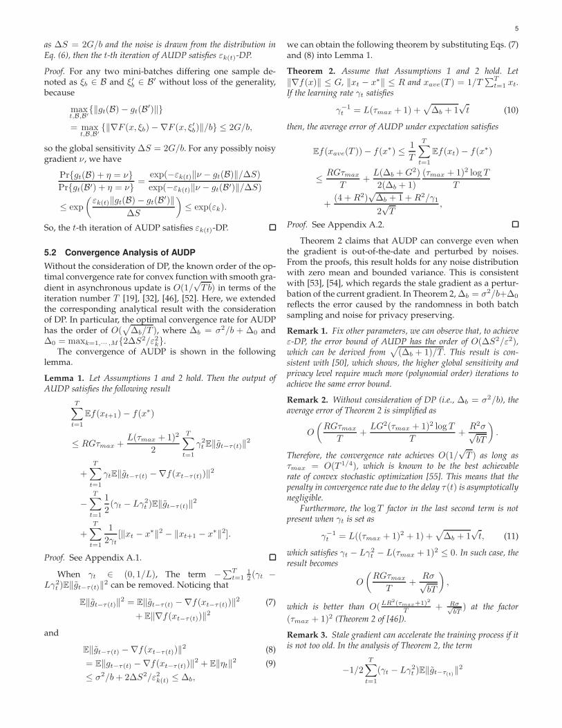
5.2 Convergence Analysis of AUDP

Without the consideration of DP, the known order of the op-timal convergence rate for convex function with smooth gra-dient in asynchronous update is O(1/

√Tb) in terms of the

iteration number T [19], [32], [46], [52]. Here, we extendedthe corresponding analytical result with the considerationof DP. In particular, the optimal convergence rate for AUDPhas the order of O(

√

∆b/T ), where ∆b = σ2/b + ∆0 and∆0 = maxk=1,··· ,M2∆S2/ε2k.

The convergence of AUDP is shown in the followinglemma.

Lemma 1. Let Assumptions 1 and 2 hold. Then the output ofAUDP satisfies the following result

T∑

t=1

Ef(xt+1)− f(x∗)

≤ RGτmax +L(τmax + 1)2

2

T∑

t=1

γ2t E‖gt−τ(t)‖2

+T∑

t=1

γtE‖gt−τ(t) −∇f(xt−τ(t))‖2

−T∑

t=1

1

2(γt − Lγ2

t )E‖gt−τ(t)‖2

+T∑

t=1

1

2γt[‖xt − x∗‖2 − ‖xt+1 − x∗‖2].

Proof. See Appendix A.1.

When γt ∈ (0, 1/L), The term −∑Tt=1

12 (γt −

Lγ2t )E‖gt−τ(t)‖2 can be removed. Noticing that

E‖gt−τ(t)‖2 = E‖gt−τ(t) −∇f(xt−τ(t))‖2 (7)

+ E‖∇f(xt−τ(t))‖2

and

E‖gt−τ(t) −∇f(xt−τ(t))‖2 (8)

= E‖gt−τ(t) −∇f(xt−τ(t))‖2 + E‖ηt‖2 (9)

≤ σ2/b+ 2∆S2/ε2k(t) ≤ ∆b,

we can obtain the following theorem by substituting Eqs. (7)and (8) into Lemma 1.

Theorem 2. Assume that Assumptions 1 and 2 hold. Let

‖∇f(x)‖ ≤ G, ‖xt − x∗‖ ≤ R and xave(T ) = 1/T∑T

t=1 xt.If the learning rate γt satisfies

γ−1t = L(τmax + 1) +

√

∆b + 1√t (10)

then, the average error of AUDP under expectation satisfies

Ef(xave(T ))− f(x∗) ≤ 1

T

T∑

t=1

Ef(xt)− f(x∗)

≤ RGτmax

T+

L(∆b +G2)

2(∆b + 1)

(τmax + 1)2 logT

T

+(4 +R2)

√∆b + 1 +R2/γ1

2√T

,


Theorem 2 claims that AUDP can converge even whenthe gradient is out-of-the-date and perturbed by noises.From the proofs, this result holds for any noise distributionwith zero mean and bounded variance. This is consistentwith [53], [54], which regards the stale gradient as a pertur-bation of the current gradient. In Theorem 2, ∆b = σ2/b+∆0

reflects the error caused by the randomness in both batchsampling and noise for privacy preserving.

Remark 1. Fix other parameters, we can observe that, to achieveε-DP, the error bound of AUDP has the order of O(∆S2/ε2),which can be derived from

√

(∆b + 1)/T . This result is con-sistent with [50], which shows, the higher global sensitivity andprivacy level require much more (polynomial order) iterations toachieve the same error bound.

Remark 2. Without consideration of DP (i.e., ∆b = σ2/b), theaverage error of Theorem 2 is simplified as

O

(RGτmax

T+

LG2(τmax + 1)2 logT

T+

R2σ√bT

)

.

Therefore, the convergence rate achieves O(1/√T ) as long as

τmax = O(T 1/4), which is known to be the best achievablerate of convex stochastic optimization [55]. This means that thepenalty in convergence rate due to the delay τ(t) is asymptoticallynegligible.

Furthermore, the logT factor in the last second term is notpresent when γt is set as

γ−1t = L((τmax + 1)2 + 1) +

√

∆b + 1√t, (11)

which satisfies γt − Lγ2t − L(τmax + 1)2 ≤ 0. In such case, the

result becomes

O

(RGτmax

T+

Rσ√bT

)

,

which is better than O(LR2(τmax+1)2

T + Rσ√bT

) at the factor

(τmax + 1)2 (Theorem 2 of [46]).

Remark 3. Stale gradient can accelerate the training process if itis not too old. In the analysis of Theorem 2, the term

−1/2T∑

t=1

(γt − Lγ2t )E‖gt−τ(t)‖2

6

originally in Lemma 1 is neglected for simplicity, which, however,can be used to eliminate part of other terms to reduce the errorbound if ‖gt−τ(t)‖ has a lower bound.

In fact, the lower bound can be commonly hold in the begin-ning of learning when the model is far away from the optimum.But if the lower bound still holds when the model is closeenough to the optimum, the stale gradient will then harm theconvergence. This means that too large staleness is not allowed inthe asynchronous update (Assumption 2). The observation that astale gradient may speed up the training is also consistent with[56].

6 MULTI STAGE ADJUSTABLE PRIVATE ALGO-

RITHM FOR ASYNCHRONOUS FEDERATED LEARN-

ING

In this section, we theoretically analyze how to estimate theglobal sensitivity and improve the model utility of the base-line algorithm AUDP. Subsequently, we propose the multistage adjustable private algorithm (MAPA) to train generalmodels by automatically adjusting the learning rate andthe global sensitivity to achieve a better trade-off betweenmodel utility and privacy protection.

6.1 Basic Idea

In AUDP, an unsolved problem is how to estimate theparameter G in Eq. (2), which is the upper bound of gra-dients norm ‖∇F (x, ξ)‖ and determines the noise scaleλ = ∆S/ε = 2G/bε. However, due to the complicatedtrained model x and the randomness of sampling ξ, it isimpossible to obtain an accurate value of G while training.Therefore, to limit the noise, many existing work proposedto clip the gradient using an fixed bound G and calibratethe privacy noise scale as 2G/bε. Nonetheless, this does notconsider the fact that the gradients norm decreases with thetraining process and will lead to either an overestimatedor underestimated estimation, as shown in Fig. 3 (a)-(c).For example, if G is larger than G, the global sensitivity∆S = 2G/b will incur too more noise to the gradients,leading to a poor model accuracy (Fig. 3 (b)). If G is muchsmaller than G, clipping may destroy the unbiasedness ofthe gradient estimate, also leading to a poor model accuracy(Fig. 3 (c)). Although an adaptive clipping method is pro-posed in [41], it remains unclear how to set the learning ratesbased on the introduced noises to ensure the model conver-gence, making its adaptive method meaningless when thetraining is not convergent.

To this end, we theoretically analyze the convergence ofAFL with DP and study the relationship between the learn-ing rate and AFL model convergence under DP. Inspired bythe relationship, we propose an adaptive clipping methodto improve the model accuracy of AUDP by changing thelearning rates to ensure the gradients norm decreases belowan expected level after some iterations. After reaching theexpected level, we adjust the learning rate once again tomake the gradient norm further converge. According todifferent learning rates, the training process is divided intodifferent stages (Fig. 3 (d)). By suppressing the gradientsnorm stage-wise, we can reduce the noises and improvethe model utility while still providing the sufficient privacyprotection.

6.2 Adaptive Gradient Bound Estimation

We first show how to estimate the global sensitivity ∆S atthe beginning.

Theorem 3. For any failure probability 0 < δ < 1, if the globalsensitivity ∆S satisfying

(1− 4σ2/(b2∆S2)

)2 ≥ 1− δ, (12)

then the t-th iteration of AUDP satisfies (εk(t), δ)-DP, where k(t)means the noisy gradient is received from the k(t)-th edge server.

Proof. For any two adjacent mini-batches differing the lastsample, we have

Pr‖gt(B)− gt(B′)‖ ≤ ∆S= Pr E‖∇F (x, ξn)−∇F (x, ξ′n)‖ ≤ b∆S≥ PrE‖∇F (x, ξn)−∇f(x)‖+ E‖∇f(x)−∇F (x, ξ′n)‖ ≤ b∆S≥ PrE‖∇F (x, ξn)−∇f(x)‖ ≤ b∆S/2·PrE‖∇F (x, ξ′n)−∇f(x)‖ ≤ b∆S/2≥

(1− 4σ2/(b2∆S2)

)2.

So, according to Theorem 1, if the sensitivity satisfiesEq. (12), the output of AUDP is εk(t)-DP with probability1− δ. In other words, AUDP guarantees (εk(t), δ)-DP.

The Cloud server can set different ∆S to satisfy differentrequirement (i.e., the failure probability δ) of edge serversbased on Theorem 3. However, ∆S may be quite larger thanthe actual global sensitivity and will introduce predominantnoise to gradients, possibly leading to the failure of modelconvergence. Therefore, to begin with a large global sensi-tivity ∆S, we should adjust and update ∆S dynamicallyto ensure the model convergence while guaranteeing theprivacy. In particular, considering that gradient convergeswith the convergence of model, we first analyze the conver-gence of the gradient. Theorem 4 shows that we can adjustthe learning rate to ensure the convergence of the gradientnorm.

Theorem 4. Assume that Assumptions 1 and 2 hold. If thelearning rate γt is a constant γ satisfying

γ−1 ≥ 2L(τmax + 1), (13)

then the output of AUDP satisfies the following result

mint∈1,··· ,T

E‖∇f(xt)‖2 ≤1

T

T∑

t=1

E‖∇f(xt)‖2

≤ 2(f(x1)− f(x∗))

Tγ+ 2∆bLγ. (14)


Theorem 4 shows that AUDP algorithm can convergeto a ball at the rate O(1/T ) with a constant learning rate.Therefore, the average norm of gradient must have a up-per bound relate to ∆b after sufficient iterations. Recall∆b = σ2/b + ∆0, i.e., the radius of the ball consists of twoparts: sampling variance σ2/b and noise variance ∆0. Dueto Theorem 3, ∆0 is inversely proportional to b. Meanwhile,sampling variance σ2/b is also inversely proportional to b.

7

Fig. 3. Illustration of multi stage adjustable DP mechanism.

Therefore, we can increase the mini-batch size to reduce theradius to control the upper bound.

In the following, we illustrate how to use Theorem 4to set the learning rate to reduce the global sensitivitygradually. Let the learning rate be

γ = 1/(2PL(τmax + 1)),

where P is an undetermined coefficient and P ≥ 1 satisfiesEq.(13). Then, the right hand side of Eq. (14) becomes

4PL(τmax + 1)(f(x1)− f(x∗))

T+

∆b

P (τmax + 1).

Let the first term be less than ∆b

P (τmax+1) , we can derive that

T ≥ T0 =4P 2L(τmax + 1)2(f(x1)− f(x∗))

∆b. (15)

Then the right hand side of Eq. (14) becomes2∆b

P (τmax+1) . Therefore, the upper bound of the gradi-

ent’s norm is estimated as√

2∆b/(P (τmax + 1)) and thenew global sensitivity after T0 iterations is estimated as2√

2∆b/(P (τmax + 1))/b, according to Theorem 1. Denotethe initial estimation by Theorem 3 as ∆S and the newestimation as ∆S′. Note that our purpose is to reducethe global sensitivity gradually. Therefore, making the newestimation less than the initial estimation, i.e.,

∆S′ ≤ θ∆S,

where θ ∈ (0, 1) is used to control the reduction ratio. Wefurther derive that

P ≥ 8∆b

(τmax + 1)b2∆S2θ2. (16)

Therefore, if we use the above P to set γ, ∆S is reducedto θ∆S. To avoid the randomnesses of sampling and noise,we use

√

2∆b/(P (τmax + 1)) to clip the gradient to ensure∆S2 is the new global sensitivity in the following trainingafter T0 iterations. We can repeat this process to graduallyreduce the global sensitivity while ensuring model conver-gence.

6.3 Multi Stage Adjustable Private Algorithm (MAPA)

With the above analysis, we propose the Multi-Stage Ad-justable Private Algorithm (MAPA) to adjust the globalsensitivity and the learning rate dynamically according tothe varying gradient during the training process to achieve a

better model utility without complicated parameter tuning.The formal description of MAPA is shown in Algorithm 1.We give the explanations as follows.

• In the initialization phase (t = 1), all edge serverssend their privacy budget εk (k = 1, ...,K) to theCloud server, which then identifies the minimal pri-vacy budget ε0 and initializes the model xt and ∆Saccording to Theorem 3. (Line 1 on the edge serverand Lines 1∼4 on the Cloud server)

• The process on the Cloud server is divided into dif-ferent stages. From the beginning, the Cloud serverruns in the first stage. In each stage, the Cloud servercomputes the intermediate parameter P , the learningrate γ, and the needed iteration number Ts for thecurrent stage. (Lines 6∼8 on the Cloud server)

• Once the training begins, each edge server pullsdown the model xt and ∆S from the Cloud server,and computes the gradient gt on the local mini-batch.Then, it clips and perturbs the gradient as gt, whichis sent to the Cloud server with privacy protection.Since the edge servers are heterogeneous in com-putation and communication, they would generallycomplete these procedures independently in differ-ent time. (Lines 3∼8 on the edge server)

• In each stage, once the Cloud server receives a stalegradient gt−τ(t) from any edge server k(t), they willupdate the model xt immediately and sends theupdated model xt and the current global sensitivity∆S to the corresponding edge sever k(t). The processrepeats until the model is updated by Ts times, whichmeans the current stage finishes and the Cloud serverwill turn into the next stage. (Lines 10∼14 on theCloud server)

• Once the Cloud server finishes the training the cur-rent stage, it will set the global sensitivity goal to bereduced as ∆S = θ∆S and computes the variance∆b, then turns into the next stage. (Lines 15∼16 onthe Cloud server)

• After the model updated by sufficient iterations (i.e.,t ≥ T ), the Cloud server finishes the training andbroadcasts the Halt command to all edge servers.(Line 18 on the Cloud server)

Remark 4. MAPA is differentially private. Because we useb∆S/2 to clip the gradient, so the global sensitivity is ∆S.Therefore, the t-th iteration in MAPA is εk(t)-DP. We don’t

8

Algorithm 1: Multi Stage Adjustable Private Algorithm(MAPA)

Input: number of edge servers K and iterations T ,mini-batch size b, reduction ratio θ, privacylevel εk, and probability δ.

Output: final model xT .// (k-th) Edge Server Side

1 Send εk to the Cloud server;2 while not Halt do3 Pull down xt and ∆S from the Cloud server;4 Compute the gradient gt(Bk) with |Bk| = b;

5 Clip the gradient as gt = gt/max(1, ‖gt‖2

b∆S/2);

6 Draw a noise ηt according to Eq. (6);7 Compute the noisy gradient gt = gt + ηt;8 Send gt to the Cloud server;9 end// The Cloud Server Side

1 Receive all εk from edge servers;2 Set ε0 = minε1, ..., εK;3 t = 1; // total iteration count

4 Initialize xt and ∆S (Theorem 3);5 while t ≤ T do6 Compute P according to Eq.(16);7 Set γ−1=2PL(τmax + 1);8 Compute Ts according to Eq.(15);9 ts=1; // stage iteration count

10 while Receiving gt−τ(t) and ts ≤ Ts do11 Update xt=xt − γgt−τ(t);12 Send xt, ∆S to the updating edge server;13 ts=ts+1, t=t+1;14 end15 Set ∆S=θ∆S;16 Compute ∆b=σ2/b+ 2∆S2/ε20;17 end18 Send Halt command to edge servers;19 return xt = xT .

consider the privacy of judgment ts ≤ Ts here. Indeed, this canbe guaranteed by the sparse vector technique [49].

We omit the discussion of the total privacy cost in this paper.Because the privacy budget is fixed in each iteration, the totalbudget is an accumulation of individual privacy costs in alliterations. By using the simple composition theorem, the total

budget is∑T

t=1 εk(t), which increases linearly with the numberof iterations. If we use the advanced composition theorem [49] ormoment account for Gaussian mechanism [30], then it becomes asub-linear function.

7 EVALUATION

In this section, we conducted extensive experimental studiesto validate the efficiency and effectiveness of MAPA.

7.1 Experimental Methodology

7.1.1 Simulation and Testbed Experiment Implementations

For a thorough evaluation, MAPA was implemented in bothMatlab and Python for simulations and testbed experimentsrespectively. Codes are available in github.com [57]. Specif-ically, we encapsulated MAPA’s Python implementations in

docker containers3 for the edge servers and the Cloud serverrespectively. To verify MAPA’s performance in practical AFLscenarios with different scales, different numbers (from 5to 20) of container-based edge servers were deployed on alocal workstation (with a 10-core CPU and 128 GB memory).The container-based Cloud server was deployed on a virtualmachine (with a 24-core CPU and 256 GB memory) of theAlibaba Cloud4. Communications between each edge serverand the Cloud server were based on Eclipse Mosquitto5

through the Internet.To set up the staleness in AFL, we adopted the cyclic

delayed method [52] for simulations, where the maximumdelay of edge-cloud communications equals the total num-ber of edge servers. For testbed experiments, the actualstaleness caused by heterogeneous delays between differentedge servers and the Cloud server was adopted.

7.1.2 Learning Models.

For generality, we applied MAPA to three machine learningmodels: Logistic Regression (LR) for a 2-way classifier;Support Vector Machine (SVM) and Convolutional NeuralNetwork (CNN) for a 10-way classifier. It should be notedthat although our theoretical results are derived based ondifferentiable convex functions (for LR), we will show thatMAPA is also applicable to non-differentiable (for SVM) andnon-convex (for CNN) loss functions. In particular, CNNconsists of five layers (two convolutional layers, two poolinglayers, and one full connection layer), noise is only addedto the gradient of the first convolutional layer, which stillguarantees differential privacy for whole CNN model dueto the post-processing property of DP [49].

7.1.3 Datasets.

We adopted two commonly-used image datasets USPS andMNIST in our evaluations. USPS contains 9,298 gray-scaleimages with 256 features (7,291 images for training and2,007 images for testing). MNIST contains 70,000 gray-scaleimages with 784 features (60,000 for training and 10,000 fortesting).

7.1.4 Comparison Algorithms and Parameter Settings.

For comprehensive evaluations, we compared MAPA (Al-gorithm 1) with the baseline algorithm AUDP to showthe utility improvement. Besides, we also compared MAPAwith the state-of-the-art asynchronous learning algorithm,the asynchronous Stochastic Gradient Descent Algorithms(ASGD) [46], [52] in terms of fast convergence speed. Also,the standard centralized Stochastic Gradient Descent algo-rithm without privacy protection, denoted as CSGD, is alsocompared for reference.

The compared algorithms with their detailed parameterssettings, such as learning rates and global sensitivities, areall listed in Table 2. For all algorithms, the regularizedparameter was set as λ = 0.0001. Without a particularexplanation, the number of edge servers K was set as 5,and the mini-batch size was set as 12. Additionally, θ wasset as 0.5 in MAPA.

3. https://www.docker.com/4. https://www.alibabacloud.com/product/ecs5. https://hub.docker.com/ /eclipse-mosquitto

9

TABLE 2Comparison Algorithms and Parameters

Algorithm Description learning rate (γ−1t ) global sensitivity (∆S)

CSGD Centralized stochastic gradient descent [55] γ−1t =L+

√t+ 1 · σ/(R

√b) N/A

MAPA Multi stage adjustable private algorithmStage s+ 1: γ−1 = 2PL(τmax + 1),

where P=max

8∆b

(τmax+1)b2∆S2sθ

2 , 1

Initial value ∆S0: by Eq.(12)Stage s+ 1: ∆Ss+1 = 2

√∆s/b

AUDP Asynchronous update with differential privacy γ−1t = L(τmax + 1) +

√∆b + 1

√t Determined by actual model

ASGD Asynchronous stochastic gradient descent [46] γ−1t =L(τmax + 1)2 +

√t+1·σ

R√

bN/A

7.2 Simulation Results

In this section, we conducted MATLAB simulation for ourproposed MAPA to demonstrate its effectiveness of privacypreserving, validate its trade-off between the model utilityand privacy, as well as the efficiency in model convergence.

7.2.1 Demonstration of Privacy Protection

This subsection demonstrates the privacy-preserving effectsand adaptive clipping bounds effects in the training processof MAPA.

To show the privacy-preserving effect, two models, LRand SVM6, were trained on MNIST and the privacy budgetin each iteration of MAPA was set as 0.01, 0.1 and 1 re-spectively. The iteration number ranges from 2000 to 14,000.To measure the privacy-preserving effects, we adopted theinferring method in [58] to recover the digital images fromthe gradients during the iterations. Fig. 4 illustrates theinferred digital images under different levels of differentialprivacy. As shown in both LR and SVM, when the privacyis higher (i.e., ε = 0.01), the inferred images are totallyblurred compared with the original image, which showsMAPA can be resilient to the inference attack; when theprivacy is lower (i.e., ε = 1), some inferred images canbe approximately restored, which also shows the privacyprotection degrades with the increase of privacy budget ε.Therefore, with proper choice of privacy budget, MAPAcan effectively control the privacy protection for the AFLsystem.

To show the adaptive bound clipping effect, LR wastrained on USPS for 100 edge servers and the privacybudget in each iteration of AUDP and MAPA was set as0.1. Fig. 5 demonstrates how the gradient norm varieswith the iteration number. In particular, Fig. 5(a) shows thegeneral gradient evolution of ASGD without DP, where the

learning rate was set as γ−1t = L(τmax + 1)2 +

√t+1·σR√b

. Fig.

5(b) illustrates the clipped gradients for AUDP with threedifferent clipping bounds, 15, 3 and 0.2. As we can see, eithertoo high or too low clipping bound would cause utilityloss. Instead, a good model utility can be achieved whenthe clipping bound is set appropriate. However, this is hardto estimate before training. Fig. 5(c) draws the results forMAPA using different initial clipping bounds 200, 100 and10, respectively. As shown, MAPA can adaptively adjust theglobal sensitivity dynamically in the training process andobtain nearly the same converged model utility as AUDP,regardless of the initial estimation of the global sensitivity.

6. For simplicity, we omitted the demonstration results for CNN.

7.2.2 Model Accuracy vs. Privacy Guarantee

In this subsection, we study the impacts of different privacylevels on the model utility. In particular, we simulated anedge-cloud FL system with five edge servers, where threemodels LR, SVM and CNN were trained for a given numberof iterations (i.e., 15,000 for LR, 10,000 for SVM and 25,000for CNN) on training datasets with the privacy budget ineach iteration ranging from 0.1 to 0.5. Then the averageprediction accuracy on testing datasets is collected.

Fig. 6 compares the model accuracy of MAPA with thebaseline algorithm AUDP under different levels of privacy.The results on both non-private algorithms CSGD andASGD are also compared for reference. As we can see,firstly, both the prediction accuracy of privacy-preservingalgorithms MAPA and AUDP increase with the differentialprivacy budget ε, which shows the genuine trade-off be-tween the model accuracy and the privacy guarantee.

Secondly, MAPA can effectively improve the predictionaccuracy of AUDP in all sub-figures for different ε and theimprovement is more significant for small privacy regimes.Especially, the maximal improvement can reach 20% in Fig.6(c) and even 100% in Fig. 6(f). This shows that MAPA canachieve a better trade-off by effectively reducing the noiseneeded for privacy guarantee.

Thirdly, MAPA can achieve a similar prediction accuracyas the non-private ASGD in all subplots with the increase ofprivacy budget. Particularly, for LR, the prediction accuracyof MAPA is even higher than ASGD. That is because theprediction accuracy of LR is mostly decided by the initiationphase and is very sensitive to the learning rate. Meanwhile,MAPA has a larger learning rate than ASGD at the begin-ning phase, leading to higher accuracy. In summary, MAPAcan achieve much higher model utility with a sufficientdifferent privacy guarantee.

7.2.3 Model Convergence vs. Edge Staleness

In this subsection, we study the impact of edge stalenesson the model convergence efficiency. We simulated threelearning models (LR, SVM, and CNN) on the edge-cloudcollaborative FL with different numbers of edge servers,e.g., K = 10, 100, 1000, respectively. In all simulations, theprivacy budget in each iteration is ε=0.1 for MAPA andAUDP, then the average number of iterations for sufficientconvergence (e.g., the average loss of 5 successive iterationsis less than a given threshold) of all algorithms were re-ported.

Fig. 7 shows the iteration number of MAPA in compari-son with both the private algorithm AUDP and non-privatealgorithms ASGD and CSGD under the different number

10

(a) LR on MNIST (b) SVM on MNIST

Fig. 4. Inference results under different privacy levels.

(a) AUDP without DP (b) AUDP with different fixed clipping bounds (c) MAPA with different initial clippingbounds

Fig. 5. Inference results between AUDP and MAPA with different clipping bounds.

0.15 0.25 0.35 0.45Privacy budget in each iteration

0.9

0.95

1

Pre

dict

ion

accu

racy

CSGDMAPA

AUDPASGD

(a) LR on MNIST

0.1 0.2 0.3 0.4 0.5Privacy budget in each iteration

0.6

0.7

0.8

0.9

1

Pre

dict

ion

accu

racy

CSGDMAPA

AUDPASGD

(b) SVM on MNIST


0.8

0.85

0.9

0.95

1

Pre

dict

ion

accu

racy

CSGDMAPA

AUDPASGD

(c) CNN on MNIST


0.92

0.94

0.96

0.98

1

Pre

dict

ion

accu

racy

CSGDMAPA

AUDPASGD

(d) LR on USPS


0.6

0.7

0.8

0.9

1

Pre

dict

ion

accu

racy

CSGDMAPA

AUDPASGD

(e) SVM on USPS


0.4

0.6

0.8

1

Pre

dict

ion

accu

racy

CSGDMAPA

AUDPASGD

(f) CNN on USPS

Fig. 6. Prediction accuracy vs. privacy budget ε.

11

x

10 100 1000Number of edge servers

102

104

106

Num

ber

of it

erat

ions

CSGDMAPA

AUDPASGD

(a) LR on MNIST (0.4)

x


104

106

Num

ber

of it

erat

ions

CSGDMAPA

AUDPASGD

(b) SVM on MNIST (0.1)

x


104

106

Num

ber

of it

erat

ions

CSGDMAPA

AUDPASGD

(c) CNN on MNIST (0.1)

x


105

Num

ber

of it

erat

ions

CSGDMAPA

AUDPASGD

(d) LR on USPS (0.2)

x


104

106

Num

ber

of it

erat

ions

CSGDMAPA

AUDPASGD

(e) SVM on USPS (0.05)

x


104

106

Num

ber

of it

erat

ions

CSGDMAPA

AUDPASGD

(f) CNN on USPS (0.1)

Fig. 7. Number of iterations for convergence vs. the number of edge servers.

of edge servers, which also represents different levels ofedge staleness. As we can see, firstly, the number of iter-ations for all asynchronous algorithms, MAPA, AUDP andASGD, increases with the number of edge servers K . Thisis because that, as K increases, the gradients used in SGDare generally staler and contain very limited information,which therefore requires more iterations for convergence.The algorithm CSGD is performed on the central Cloudwithout collaborations with the edges and requires muchfewer iterations.

Secondly, MAPA achieves a faster convergence speedthan AUDP. When K=10 and 100, MAPA can save 1-2amplitudes of the number of iterations. For example, whenK=10 in Fig. 7(a), 2 amplitude saving is achieved. Thereason is that the adjustable noise scale and learning ratetogether can ensure the model converges at the rate O(1/T )(Theorem 4) in each stage.

Thirdly, MAPA achieves a faster convergence speed thanASGD and saved about 2 amplitude when K=100 and1000. The reason is that a linear decaying learning ratewith respect to K (i.e., the τmax) is used in MAPA, butin ASGD, a second power polynomial decaying learningrate is designed to alleviate the effects of the staleness.However, as K increases, the quickly decaying learning notonly alleviates the staleness but also the useful informationtoo much, leading to a long training process. In summary,MAPA can effectively tackle the edge staleness problem andhave a better convergence efficiency for AFL.

7.3 Testbed Experiment Results

In this section, we verify the practical performance of MAPAbased on real-world testbed experiments, as a complementto the simulations. Furthermore, the impacts of learning

parameters on the practical performance of MAPA werevalidated. For simplicity, only the results of CNN model onthe MNIST dataset are reported.

7.3.1 Model Utility

We implemented MAPA to train a CNN model in the testbedAFL system with the different number of edge servers Kas 5, 10, 15, and 20, respectively. The average predictionaccuracy of trained models under different iterations on theedge servers are reported and drawn in Fig. 8.

As shown, the prediction accuracy of MAPA is higherthan AUDP in all cases. Also, with the increase of edgenumber, MAPA can even effectively outperform the non-private ASGD. These observations are consistent with thesimulation results and validate the utility improvementof MAPA in practical systems. Secondly, both MAPA andAUDP can obtain almost the same prediction accuracy asCSGD for CNN model training. That shows, adding propernoise will not significantly impact the model utility of CNN.As pointed out in [49], appropriate random noises playthe role of the regularization in machine learning and canenhance the robustness of the trained model.

7.3.2 Impacts of Parameters

In this subsection, we demonstrated the impact of learningparameter on the model utility of MAPA in real-worldtestbed AFL system. When considering the impact of anindividual parameter, others were fixed as default value,i.e., ε = 0.1, b = 12, σ = 30, L = 10, δ = 10−3, θ = 1/2.

Fig. 9 shows the prediction accuracy of the trained modelwith MAPA concerning different parameters. We can havethe following observations. Firstly, Figs. 9(c) and 9(e) showthat MAPA is robust to both σ and δ. That is, the estimation

12

of the sample variance and the setting of probability lossare not crucial for convergence. Secondly, batch size andsmooth constant have a little impact on prediction accuracy.For example, in Figs. 9(b) and 9(d), using a larger mini-batchsize b and smaller smooth constant L can achieve a fasterspeed at the beginning, but will finally trend to the sameaccuracy at the given iterations. Thirdly, MAPA is sensitiveto not only the privacy level but also the reduction ratio.In Fig. 9(f), it is observed that a larger reduction ratio willlead to lower model accuracy. The reason is that the learningrate will be adjusted too small for sufficiently achieving thelarger reduction ratio (according to Theorem 4), leading tomuch more iterations.

0 1000 2000 3000 4000 5000Iteration number

0

0.2

0.4

0.6

0.8

1

Pre

dict

ion

accu

racy

CSGDMAPA

AUDPASGD

(a) K = 5


0

0.2

0.4

0.6

0.8

1

Pre

dict

ion

accu

racy

CSGDMAPA

AUDPASGD

(b) K = 10


0

0.2

0.4

0.6

0.8

1

Pre

dict

ion

accu

racy

CSGDMAPA

AUDPASGD

(c) K = 15


0

0.2

0.4

0.6

0.8

1

Pre

dict

ion

accu

racy

CSGDMAPA

AUDPASGD

(d) K = 20

Fig. 8. Prediction accuracy under different number of edge servers.

8 CONCLUSION

This paper presents the first study on Asynchronous edge-cloud collaboration based Federated Learning (AFL) withdifferential privacy. Based on a baseline algorithm, we firsttheoretically analyzed the impact of differential privacy onthe convergence of AFL. To enhance the learning utility, wethen propose a Multi-Stage Adjustable Private Algorithm(MAPA) for AFL, which can adaptively clip the gradientsensitivity to reduce the privacy-preserving noise, thusachieving high model accuracy without complicated param-eter tuning. We applied our proposed algorithms to severalmachine learning models, and validated their performancevia both Matlab simulations and real-world testbed exper-iments. The experimental results show that, in comparisonwith the state-of-the-art AFL algorithms, MAPA can achievenot only much better trade-off between the model utilityand privacy guarantee but also much higher convergenceefficiency.

REFERENCES

[1] B. Hu, Z. Lu, H. Li, and Q. Chen, “Convolutional neural networkarchitectures for matching natural language sentences,” in Proc. ofNeurIPs, 2014, pp. 2042–2050.


0

0.2

0.4

0.6

0.8

1

Pre

dict

ion

accu

racy

=0.01=0.1=1

(a) Privacy level


0

0.2

0.4

0.6

0.8

1

Pre

dict

ion

accu

racy

b=12b=32b=64

(b) Batch size

1000 2000 3000 4000 5000Iteration number

0.2

0.4

0.6

0.8

1

Pre

dict

ion

accu

racy

=10=30=50

(c) Sample variance


0

0.2

0.4

0.6

0.8

1

Pre

dict

ion

accu

racy

L=10L=15L=20

(d) Lipschitz smooth constant


0

0.2

0.4

0.6

0.8

1

Pre

dict

ion

accu

racy

=10-3

=10-4

=10-5

(e) Probability loss


0

0.2

0.4

0.6

0.8

1

Pre

dict

ion

accu

racy

=1/4=2/4=3/4

(f) Reduction ratio

Fig. 9. Prediction accuracy with respect to different parameters.

[2] W. Hu, G. Tian, Y. Kang, C. Yuan, and S. Maybank, “Dual stickyhierarchical dirichlet process hidden markov model and its ap-plication to natural language description of motions,” IEEE Trans.Pattern Anal. Mach. Intell., vol. 40, no. 10, pp. 2355–2373, Oct 2018.

[3] F. Wan, P. Wei, Z. Han, J. Jiao, and Q. Ye, “Min-entropy latentmodel for weakly supervised object detection,” IEEE Trans. PatternAnal. Mach. Intell., vol. 41, no. 10, pp. 2395–2409, Oct 2019.

[4] Z. Shen, Z. Liu, J. Li, Y. Jiang, Y. Chen, and X. Xue, “Objectdetection from scratch with deep supervision,” IEEE Trans. PatternAnal. Mach. Intell., pp. 1–1, 2019.

[5] J. Lu, V. E. Liong, X. Zhou, and J. Zhou, “Learning compact binaryface descriptor for face recognition,” IEEE Trans. Pattern Anal.Mach. Intell., vol. 37, no. 10, pp. 2041–2056, Oct 2015.

[6] C. Ding and D. Tao, “Trunk-branch ensemble convolutional neuralnetworks for video-based face recognition,” IEEE Trans. PatternAnal. Mach. Intell., vol. 40, no. 4, pp. 1002–1014, April 2018.

[7] R. Shokri and V. Shmatikov, “Privacy-preserving deep learning,”in Proc. of ACM CCS. ACM, 2015, pp. 1310–1321.

[8] P. Mohassel and Y. Zhang, “Secureml: A system for scalableprivacy-preserving machine learning,” in IEEE Security Privacy.IEEE, 2017, pp. 19–38.

[9] H. B. McMahan, D. Ramage, K. Talwar, and L. Zhang, “Learningdifferentially private recurrent language models,” in ICLR, 2018.

[10] Q. Zhang, L. T. Yang, and Z. Chen, “Privacy preserving deepcomputation model on cloud for big data feature learning,” IEEETrans. Comput., vol. 65, no. 5, pp. 1351–1362, May 2016.

[11] Q. Yang, Y. Liu, T. Chen, and Y. Tong, “Federated machine learn-ing: Concept and applications,” ACM Transactions on IntelligentSystems and Technology, vol. 10, no. 2, p. 12, 2019.

[12] P. Voigt and A. Von dem Bussche, The EU General Data ProtectionRegulation (GDPR). Springer, 2017, vol. 18.

[13] J. Konecny, H. B. McMahan, F. X. Yu, P. Richtarik, A. T. Suresh,and D. Bacon, “Federated learning: Strategies for improving com-munication efficiency,” CoRR, vol. abs/1610.05492, 2016.

[14] B. McMahan, E. Moore, D. Ramage, S. Hampson, and B. A. y Ar-cas, “Communication-efficient learning of deep networks from

13

decentralized data,” in Artificial Intelligence and Statistics, 2017, pp.1273–1282.

[15] J. Konecny, H. B. McMahan, D. Ramage, and P. Richtarik, “Fed-erated optimization: Distributed machine learning for on-deviceintelligence,” arXiv preprint arXiv:1610.02527, 2016.

[16] D. Liu, T. Miller, R. Sayeed, and K. Mandl, “Fadl: Federated-autonomous deep learning for distributed electronic healthrecord,” arXiv preprint arXiv:1811.11400, 2018.

[17] G. Wang, “Interpret federated learning with shapley values,” arXivpreprint arXiv:1905.04519, 2019.

[18] W. Yang, Y. Zhang, K. Ye, L. Li, and C.-Z. Xu, “Ffd: A federatedlearning based method for credit card fraud detection,” in Interna-tional Conference on Big Data. Springer, 2019, pp. 18–32.

[19] B. Recht, C. Re, S. Wright, and F. Niu, “Hogwild: A lock-freeapproach to parallelizing stochastic gradient descent,” in Proc. ofNeurIPs, 2011, pp. 693–701.

[20] J. Liu and S. J. Wright, “Asynchronous stochastic coordinate de-scent: Parallelism and convergence properties,” SIAM Journal onOptimization, vol. 25, no. 1, pp. 351–376, 2015.

[21] T. Sun, R. Hannah, and W. Yin, “Asynchronous coordinate descentunder more realistic assumptions,” in Proc. of NeurIPs, 2017, pp.6182–6190.

[22] R. Zhang and J. Kwok, “Asynchronous distributed admm forconsensus optimization,” in ACM ICML, 2014, pp. 1701–1709.

[23] R. Hannah and W. Yin, “More iterations per second, same quality–why asynchronous algorithms may drastically outperform tradi-tional ones,” arXiv preprint arXiv:1708.05136, 2017.

[24] Y. Lu, X. Huang, Y. Dai, S. Maharjan, and Y. Zhang, “Differentiallyprivate asynchronous federated learning for mobile edge comput-ing in urban informatics,” IEEE Trans. Ind. Informat., pp. 1–1, 2019.

[25] M. Fredrikson, S. Jha, and T. Ristenpart, “Model inversion attacksthat exploit confidence information and basic countermeasures,”in Proc. of CCS. New York, NY, USA: ACM, 2015, pp. 1322–1333.

[26] L. Melis, C. Song, E. De Cristofaro, and V. Shmatikov, “Exploitingunintended feature leakage in collaborative learning,” in IEEES&P, May 2019, pp. 691–706.

[27] R. Shokri, M. Stronati, C. Song, and V. Shmatikov, “Membershipinference attacks against machine learning models,” in IEEE Secu-rity Privacy, May 2017, pp. 3–18.

[28] I. Giacomelli, S. Jha, M. Joye, C. D. Page, and K. Yoon, “Privacy-preserving ridge regression with only linearly-homomorphic en-cryption,” in Proc. of Springer ACNS. Springer, 2018, pp. 243–261.

[29] C. Dwork, F. Mcsherry, and K. Nissim, “Calibrating noise to sen-sitivity in private data analysis,” Proc. of Morgan Kaufmann/ACMVLDB, vol. 7, no. 8, pp. 637–648, 2006.

[30] M. Abadi, A. Chu, I. Goodfellow, H. B. McMahan, I. Mironov,K. Talwar, and L. Zhang, “Deep learning with differential privacy,”in Proc. of ACM CCS. New York, USA: ACM, 2016, pp. 308–318.

[31] R. C. Geyer, T. Klein, and M. Nabi, “Differentially private feder-ated learning: A client level perspective,” in Proc. of NeurIPs, vol.abs/1712.07557, 2017.

[32] N. Agarwal, A. T. Suresh, F. X. X. Yu, S. Kumar, and B. McMa-han, “cpsgd: Communication-efficient and differentially-privatedistributed sgd,” in Proc. of NeurIPs, 2018, pp. 7564–7575.

[33] K. Bonawitz, V. Ivanov, B. Kreuter, A. Marcedone, H. B. McMahan,S. Patel, D. Ramage, A. Segal, and K. Seth, “Practical secureaggregation for privacy-preserving machine learning,” in Proc. ofACM CCS. ACM, 2017, pp. 1175–1191.

[34] N. Papernot, M. Abadi, U. Erlingsson, I. Goodfellow, and K. Tal-war, “Semi-supervised knowledge transfer for deep learning fromprivate training data,” arXiv preprint arXiv:1610.05755, 2016.

[35] N. Papernot, P. McDaniel, A. Sinha, and M. P. Wellman, “Sok:Security and privacy in machine learning,” in Proc. of S&P. IEEE,2018, pp. 399–414.

[36] R. Bassily, A. Smith, and A. Thakurta, “Private empirical riskminimization: Efficient algorithms and tight error bounds,” in2014 IEEE 55th Annual Symposium on Foundations of ComputerScience. IEEE, 2014, pp. 464–473.

[37] K. Chaudhuri, C. Monteleoni, and A. D. Sarwate, “DifferentiallyPrivate Empirical Risk Minimization,” JOURNAL OF MACHINELEARNING RESEARCH, vol. 12, pp. 1069–1109, MAR 2011.

[38] H. B. McMahan and G. Andrew, “A general approach to addingdifferential privacy to iterative training procedures,” arXiv preprintarXiv:1812.06210, 2018.

[39] T. Chanyaswad, A. Dytso, H. V. Poor, and P. Mittal, “Mvg mecha-nism: Differential privacy under matrix-valued query,” in Proc. ofACM SIGSAC. ACM, 2018, pp. 230–246.

[40] W. Du, A. Li, and Q. Li, “Privacy-preserving multiparty learningfor logistic regression,” in Proc. of Security and Privacy in Communi-cation Systems. Springer, 2018, pp. 549–568.

[41] O. Thakkar, G. Andrew, and H. B. McMahan, “Differen-tially private learning with adaptive clipping,” arXiv preprintarXiv:1905.03871, 2019.

[42] M. Lecuyer, V. Atlidakis, R. Geambasu, D. Hsu, and S. Jana,“on the connection between differential privacy and adversarialrobustness in machine learning,” stat, vol. 1050, p. 9, 2018.

[43] K. D. P and W. M, “Auto-encoding variational bayes,” in Proc. ofNeurIPs, vol. abs/1312.6114, 2013.

[44] M. Cisse, P. Bojanowski, E. Grave, Y. Dauphin, and N. Usunier,“Parseval networks: Improving robustness to adversarial exam-ples,” in Proc. of ACM ICML. JMLR. org, 2017, pp. 854–863.

[45] L. Xiao, “Dual averaging methods for regularized stochastic learn-ing and online optimization,” Journal of Machine Learning Research,vol. 11, no. Oct, pp. 2543–2596, 2010.

[46] H. R. Feyzmahdavian, A. Aytekin, and M. Johansson, “An asyn-chronous mini-batch algorithm for regularized stochastic opti-mization,” IEEE Trans. Autom. Control, vol. 61, no. 12, pp. 3740–3754, 2016.

[47] X. Lian, Y. Huang, Y. Li, and J. Liu, “Asynchronous paral-lel stochastic gradient for nonconvex optimization,” in Proc. ofNeurIPs. Curran Associates, Inc., 2015, pp. 2737–2745.

[48] B. Hitaj, G. Ateniese, and F. Perez-Cruz, “Deep models under thegan: Information leakage from collaborative deep learning,” inProc. of ACM CCS. New York, USA: ACM, 2017, pp. 603–618.

[49] C. Dwork, A. Roth et al., “The algorithmic foundations of differ-ential privacy,” Foundations and Trends R© in Theoretical ComputerScience, vol. 9, no. 3–4, pp. 211–407, 2014.

[50] Z. Huang, S. Mitra, and N. Vaidya, “Differentially private dis-tributed optimization,” in Proc. of ACM Distributed Computing andNetworking. ACM, 2015, p. 4.

[51] M. Pathak, S. Rane, and B. Raj, “Multiparty differential privacy viaaggregation of locally trained classifiers,” in Proc. of NeurIPs, 2010,pp. 1876–1884.

[52] A. Agarwal and J. C. Duchi, “Distributed delayed stochasticoptimization,” in Proc. of NeurIPs. Curran Associates, Inc., 2011,pp. 873–881.

[53] H. Mania, X. Pan, D. Papailiopoulos, B. Recht, K. Ramchandran,and M. I. Jordan, “Perturbed iterate analysis for asynchronousstochastic optimization,” SIAM Journal on Optimization, vol. 27,no. 4, pp. 2202–2229, 2017.

[54] S. Chaturapruek, J. C. Duchi, and C. Re, “Asynchronous stochasticconvex optimization: the noise is in the noise and sgd don’t care,”in Proc. of NeurIPs. Curran Associates, Inc., 2015, pp. 1531–1539.

[55] S. Bubeck et al., “Convex optimization: Algorithms and complex-ity,” Foundations and Trends R© in Machine Learning, vol. 8, no. 3-4,pp. 231–357, 2015.

[56] I. Mitliagkas, C. Zhang, S. Hadjis, and C. Re, “Asynchrony begetsmomentum, with an application to deep learning,” in AnnualAllerton Conference on Communication, Control, and Computing.IEEE, 2016, pp. 997–1004.

[57] https://github.com/IoTDATALab/MAPA.[58] L. T. Phong, Y. Aono, T. Hayashi, L. Wang, and S. Moriai, “Privacy-

preserving deep learning via additively homomorphic encryp-tion,” IEEE Trans. Inf. Forensics Security, vol. 13, no. 5, pp. 1333–1345, 2018.

[59] L. M. Bregman, “The relaxation method of finding the commonpoint of convex sets and its application to the solution of problemsin convex programming,” USSR computational mathematics andmathematical physics, vol. 7, no. 3, pp. 200–217, 1967.

Yanan Li received his in Bachelor and Masterdegree from Henan Normal University of Chinain 2004 and 2007, respectively. He is currentlyworking towards the PhD degree in the Schoolof Mathematics and Statistics at Xi’an JiaotongUniversity. Before that, he worked as a lecturerin Henan Polytechnic University from 2007 to2017. His research interests include differentialprivacy, federated learning, and edge computing.

14

Shusen Yang received his PhD in Computingfrom Imperial College London in 2014. He is cur-rently a professor in the Institute of Informationand System Science at Xi’an Jiaotong University(XJTU). Before joining XJTU, Shusen worked asa Lecturer (Assistant Professor) at University ofLiverpool from 2015 to 2016, and a ResearchAssociate at Intel Collaborative Research Insti-tute ICRI from 2013 to 2014. His research inter-ests include mobile networks, networks with hu-man in the loop, data-driven networked systems

and edge computing. Shusen achieves “1000 Young Talents Program”award, and holds an honorary research fellow at Imperial College Lon-don. Shusen is a senior member of IEEE and a member of ACM.

Xuebin Ren received his PhD degree in the De-partment of Computer Science and Technologyfrom Xi’an Jiaotong University, China in 2017.Currently, he is a lecturer in Xi’an Jiaotong Uni-versity and a member of National EngineeringLaboratory for Big Data Analytics (NEL-BDA).He has been a visiting PhD student in the De-partment of Computing at Imperial College Lon-don from 2016 to 2017. His research interests fo-cus on data privacy protection, federated learn-ing and privacy-preserving machine learning. He

is a member of the IEEE and the ACM.

Cong Zhao received his Ph.D. degree from XianJiaotong University (XJTU) in 2017. He is cur-rently a Research Associate in the Departmentof Computing at Imperial College London. Hisresearch interests include edge computing, com-puting economics, and people-centric sensing.

15

APPENDIX A

PROOF OF THEOREMS

A.1 Proof of Lemma 1

We give a lemma before the formal proof of Lemma 1.

Lemma 2. Let Assumption 1, ‖x−x∗‖ ≤ R and ‖∇f(x)‖ ≤ Ghold. Then, we have

T∑

t=1

E〈∇f(xt)−∇f(xt−τ(t)), xt+1 − x∗〉

≤ Rcτmax +L(τmax + 1)2

2

T∑

t=1

γ2t E‖gt−τ(t)‖2.

Proof. The proof follows by using a few Bregman divergenceidentities to rewrite the inner production. Let Df (·, ·) is theBregman divergence of f [59] which is defined as

Df(x, y) := f(x)− f(y)− 〈∇f(y), x− y〉. (17)

Based on the following well-known four term equality, aconsequence of straightforward algebra: for any a, b, c, d,

〈∇f(a)−∇f(b), c− d〉= Df 〈d, a〉 −Df 〈d, b〉 −Df 〈c, a〉+Df 〈c, b〉.

We have

〈∇f(xt)−∇f(xt−τ(t)), xt+1 − x∗〉= Df (x

∗, xt)−Df (x∗, xt−τ(t))−Df (xt+1, xt)

+Df (xt+1, xt−τ(t))

≤ Df (x∗, xt)−Df (x

∗, xt−τ(t)) + L/2‖xt+1 − xt−τ(t)‖2.(18)

In the last inequality, we drop the non-negative termDf (xt+1, xt), and use

Df (xt+1, xt−τ(t)) ≤ L/2‖xtt+1 − xt−τ(t)‖2,

which is derived from Eq. (17) and smooth gradient.Taking expectation on both sides of Eq. (18), and sum-

mation t from 1 to T , we have

T∑

t=1

E〈∇f(xt)−∇f(xt−τ(t)), xt+1 − x∗〉

≤T∑

t=1

E[Df(x∗, xt)−Df (x

∗, xt−τ(t))]

+L

2

T∑

t=1

E‖k=t∑

k=t−τ(t)

xk − xk+1‖2

≤T∑

t=T−τmax+1

EDf (x∗, xt)

+L

2

T∑

t=1

(τ(t) + 1)t∑

k=t−τ(t)

E‖xk − xk+1‖2. (19)

For Bregman divergence Df(x∗, xt) in Eq. (19), we have

Df (x∗, xt) = f(x∗)− f(xt)− 〈∇f(xt), x

∗ − xt〉≤ ‖∇f(xt)‖∗‖x∗ − xt‖ ≤ RG. (20)

Next, we bound the remaining term in Eq. (19).

T∑

t=1

(τ(t) + 1)t∑

k=t−τ(t)

E‖xk − xk+1‖2

≤T∑

t=1

(τ(t) + 1)t∑

k=t−τ(t)

γ2kE‖gk−τ(k)‖2

≤ (τmax + 1)T∑

t=1

t∑

k=t−τ(t)

γ2k(E‖gk−τ(k)‖2)

≤ (τmax + 1)2T∑

t=1

γ2t (E‖gt−τ(t)‖2).

Substituting this result and Eq. (20) into Eqs. (19) completesthe proof.

Now, we prove Lemma 1.Based on the L-Lipschitz continuity of gradient and

convexity of function, we have

Ef(xt+1)− f(x∗)

≤ E〈∇f(xt), xt+1 − x∗〉+ L

2E‖xt+1 − xt‖2

= E〈∇f(xt)−∇f(xt−τ(t)), xt+1 − x∗〉︸︷︷︸

T1

+ E〈∇f(xt−τ(t))− gt−τ(t), xt+1 − x∗〉︸︷︷︸

T2

+ E〈gt−τ(t), xt+1 − x∗〉︸︷︷︸

T3

+Lγ2t /2E‖gt−τ(t)‖2. (21)

With respect to T1, by Lemma 2, we have

T∑

t=1

T1 ≤ RGτmax +L(τmax + 1)2

2

T∑

t=1

γ2t E‖gt−τ(t)‖2. (22)

With respect to T2, we have

T2 = E〈∇f(xt−τ(t))− gt−τ(t), xt+1 − xt〉+ E〈∇f(xt−τ(t))− gt−τ(t), xt − x∗〉

= E〈∇f(xt−τ(t))− gt−τ(t),−γtgt−τ(t)〉= −γtE〈∇f(xt−τ(t)), gt−τ(t)〉+ γtE‖gt−τ(t)‖2

= −γt‖∇f(xt−τ(t))‖2 + γtE‖gt−τ(t) −∇f(xt−τ(t))‖2

+ γt‖∇f(xt−τ(t))‖2

= γtE‖gt−τ(t) −∇f(xt−τ(t))‖2. (23)

The second equality in Eq. (23) follows

E〈∇f(xt−τ(t))− gt−τ(t), xt − x∗〉 = 0.

The fourth equality in Eq. (23) follows

E〈∇f(xt−τ(t)), gt−τ(t)〉 = ‖∇f(xt−τ(t))‖2,E〈gt−τ(t) −∇f(xt−τ(t)),∇f(xt−τ(t))〉 = 0.

The last equality in Eq. (23) follows

E〈gt−τ(t) −∇f(xt−τ(t)), gt−τ(t) −∇f(xt−τ(t))〉= E‖gt−τ(t)‖2 + E‖∇f(t− τ(t))‖2 − 2E‖∇f(t− τ(t))‖2.

16


T3 = E〈gt−τ(t), xt+1 − xt〉+ E〈gt−τ(t), xt − x∗〉= E〈gt−τ(t),−γtgt−τ(t)〉+ 1/γtE〈γtgt−τ(t), xt − x∗〉

= −γtE‖gt−τ(t)‖2 +1

2γtE(γ2

t ‖gt−τ(t)‖2

+ ‖xt − x∗‖2 − ‖xt+1 − x∗‖2)

= −γt2E‖gt−τ(t)‖2 +

1

2γtE[‖xt − x∗‖2 − ‖xt+1 − x∗‖2].

(24)

The third equality uses the fact 〈a, b〉 = 1/2[‖a‖2 + ‖b‖2 −‖a− b‖2].

Taking summation on both sides of Eq. (21) from 1 to T ,and replacing T1, T2, T3 with upper bound of Eqs. (22), (23)and (24), we have

T∑

t=1

Ef(xt+1)− f(x∗)

≤ RGτmax +L(τmax + 1)2

2

T∑

t=1

γ2t E‖gt−τ(t)‖2

+T∑

t=1

γtE‖gt−τ(t) −∇f(xt−τ(t))‖2

−T∑

t=1

1

2(γt − Lγ2

t )E‖gt−τ(t)‖2

+T∑

t=1

1

2γt[‖xt − x∗‖2 − ‖xt+1 − x∗‖2].

A.2 Proof of Theorem 2

When γt is set as γ−1t = L(τmax + 1) +

√∆b + 1

√t,

obviously for all t ∈ N+, γt ∈ (0, 1/L).Therefore we drop

the minus term 12

∑Tt=1

(γt − Lγ2

t

)E‖gt−τ(t)‖2. Due to

E‖gt−τ(t) −∇f(xt−τ(t))‖2

= E‖gt−τ(t) −∇f(xt−τ(t))‖2 + E‖ηt‖2

≤ σ2/b+ 2∆S2/ε2k(t) ≤ ∆b.

and

E‖gt−τ(t)‖2

= E‖gt−τ(t) −∇f(xt−τ(t))‖2 + E‖∇f(xt−τ(t))‖2

≤ ∆b +G2,

we have

1

T

T∑

t=1

Ef(xt+1)− f(x∗)

≤ RGτmax

T+

L(τmax + 1)2(∆b +G2)

2T

T∑

t=1

γ2t

+∆b

T

T∑

t=1

γt +1

T

T∑

t=1

1

2γt(‖xt − x∗‖2 − ‖xt+1 − x∗‖2).

(25)

By observing that

T∑

t=1

γ2t ≤

T∑

t=1

1

(∆b + 1)t≤ logT

∆b + 1, (26)

T∑

t=1

γt ≤T∑

t=1

1√∆b + 1

1√t≤ 2

√T√

∆b + 1, (27)

and

T∑

t=1

1

2γt(‖xt − x∗‖2 − ‖xt+1 − x∗‖2)

≤ R2

2γ1+

√∆b + 1R2/2√

T, (28)

we complete the proof after returning Eqs. (26), (27) and (28)back into Eq. (25).

A.3 Proof of Theorem 4

The essential idea is using the properties of smooth functionand several inequality to separate the gradient. Recall theupdate formula

xt+1 − xt = −γtgt−τ(t), gt−τ(t) = gt−τ(t) + ηt,

where ηt follows the density function Eq. (6),

E(η) = 0,E(‖η‖2) = 2∆S2k(t)/ε

2k(t).

Based on the Lipschitz continuity of gradient, we have

f(xt+1)− f(xt)

≤ 〈∇f(xt), xt+1 − xt〉+ L/2‖xt+1 − xt‖2

≤ −γt〈∇f(xt), (gt−τ(t))〉+ Lγ2t /2E‖gt−τ(t)‖2.

Taking expectation respect to ηt and ξ, we have

E〈∇f(xt), (gt−τ(t))〉 = 〈∇f(xt),∇f(xt−τ(t))〉

=1

2

(‖∇f(xt)‖2 + ‖∇f(xt−τ(t))‖2

−‖∇f(xt)−∇f(xt−τ(t))‖2),

where we use the unbiased estimation in the first equalityand the second equality uses the fact that

〈a, b〉 = 1

2

(‖a‖2 + ‖b‖2 − ‖a− b‖2

).

So we have

E[f(xtt+1)− f(xt)]

≤ −γt2

(‖∇f(xt)‖2 + ‖∇f(xt−τ(t))‖2

− ‖∇f(xt)−∇f(xt−τ(t))‖2︸︷︷︸

T1

) + Lγ2t /2E‖gt−τ(t)‖2

︸︷︷︸

T2

. (29)

Next we estimate the upper bound of T1 and T2. For T2, wehave

T2 = E‖gt−τ(t)‖2

= E‖gt−τ(t) −∇f(xt−τ(t)) +∇f(xt−τ(t))‖2

= E‖gt−τ(t) −∇f(xt−τ(t))‖2 + E‖∇f(xt−τ(t))‖2

= E‖gt−τ(t) −∇f(xt−τ(t))‖2 + E‖ηt‖2 + E‖∇f(xt−τ(t))‖2

≤ σ2/b+ 2∆S2k(t)/ε

2k(t) + E‖∇f(xt−τ(t))‖2

≤ ∆b + E‖∇f(xt−τ(t))‖2, (30)

17

where the third equality is due to

Eξ|ηt〈Eηt

gt−τ(t) −∇f(xt−τ(t)),∇f(xt−τ(t))〉= Eξ〈gt−τ(t) −∇f(xt−τ(t)),∇f(xt−τ(t))〉= 〈Eξgt−τ(t) −∇f(xt−τ(t)),∇f(xt−τ(t))〉 = 0

and the fourth equality is due to

E‖gt−τ(t) −∇f(xt−τ(t))‖2

= E‖gt−τ(t) −∇f(xt−τ(t)) + ηt‖2

= E‖gt−τ(t) −∇f(xt−τ(t))‖2 + E‖ηt‖2

≤ σ2/b+ 2∆S2k/ε

2k.


T1 = ‖∇f(xt)−∇f(xt−τ(t))‖2 ≤ L2‖xt − xt−τ(t)‖2

= L2‖t−1∑

j=t−τ(t)

xj+1 − xj‖2 = L2‖t−1∑

j=t−τ(t)

γj gj−τ(j)‖2

≤ 2L2 ‖t−1∑

j=t−τ(t)

γj(gj−τ(j) −∇f(xj − τ(j))

)‖2

︸︷︷︸

T3

+ 2L2 ‖t−1∑

j=t−τ(t)

γj∇f(xj − τ(j))‖2

︸︷︷︸

T4

(31)

where the last inequality is derived from the fact that ‖a‖2 =‖a− b+ b‖2 ≤ ‖a− b‖2 + ‖b‖2. With respect to T3, we have

ET3 = Eξ|ηj(Eηj

T3)

= E

t−1∑

j=t−τ(t)

γ2j ‖gj−τ(j) −∇f(xj−τ(j))‖2

= E

t−1∑

j=t−τ(t)

γ2j

(‖gj−τ(j) −∇f(xj−τ(j))‖2 + E‖ηj‖2

)

≤ E

t−1∑

j=t−τmax

γ2j

(‖gj−τ(j) −∇f(xj−τ(j))‖2 + E‖ηj‖2

)

≤t−1∑

j=t−τmax

γ2j

(

σ2/b+ 2∆S2k(j)/ε

2k(j)

)

≤ ∆b

t−1∑

j=t−τmax

γ2j .


ET4 ≤ τ(t)t−1∑

j=t−τ(t)

γ2j ‖∇f(xj−τ(j))‖2

≤ τmax

t−1∑

j=t−τmax

γ2j ‖∇f(xj−τ(j))‖2

Taking full expectation on both sides of Eq. (31) and replac-ing ET3 and ET4 with their upper bound, we have

ET1 ≤ 2L2

∆b

t−1∑

j=t−τmax

γ2j

+τmax

t−1∑

j=t−τmax

γ2j ‖∇f(xj−τ(j))‖2

. (32)

Taking Eqs. (32) and (30) back into Eq. (29), we have

Ef(xt+1)− f(xt)

≤ −γt2

(E‖∇f(xt)‖2 + E‖∇f(xt−τ(t))‖2

)

+ L2γt

∆b

t−1∑

j=t−τmax

γ2j + τmax

t−1∑

j=t−τmax

γ2jE‖∇f(xj−τ(j))‖2

+Lγ2

t

2

(∆b + E‖∇f(xt−τ(t))‖2

)

≤ −γt2E‖∇f(xt)‖2 +

(Lγ2

t − γt2

)

E‖∇f(xt−τ(t))‖2

+∆b

Lγ2

t

2+ L2γt

t−1∑

j=t−τmax

γ2j

+ L2γtτmax

t−1∑

j=t−τmax

γ2jE‖∇f(xj−τ(j))‖2.

Taking summation on t from 1 to T and rearranging terms,we have

Ef(xT+1)− f(x1)

≤ −1

2

T∑

t=1

γtE‖∇f(xt)‖2

+T∑

t=1

γ2t (

L

2+ L2τmax

τmax∑

ρ=1

γt+ρ)−γt2

E‖∇f(xt−τ(t))‖2

+∆b

T∑

t=1

Lγ2

t

2+ L2γt

t−1∑

j=t−τmax

γ2j

.

If γt is set as a constant 1/(2L(τmax + 1)) (Eq. (13)), then

γ2t

L

2+ L2τmax

τmax∑

ρ=1

γt+ρ

− γt2

< 0

is always hold. Dropping this minus term and taking sum-mation on t from 1 to T , we have

T∑

t=1

γE‖∇f(xt)‖2 ≤ 2(f(x1)− f(x∗))

+ ∆b

T∑

t=1

(Lγ2 + 2L2γ3τmax

),

where we ue the fact that f(x1)−f(xT+1) ≤ f(x1)−f(x∗).Dividing T on both sides with γT , we have

1

T

T∑

t=1

E‖∇f(xt)‖2 ≤2(f(x1)− f(x∗)) + ∆bT 2Lγ

2

Tγ,

in where 2L2γ3τmax ≤ Lγ2. Therefore,

1

T

T∑

t=1

E‖∇f(xt)‖2 ≤2(f(x1)− f(x∗))

Tγ+ 2∆bLγ

completes the proof.

Documents

1 Asynchronous Federated Learning with Differential