1

An Integrated Sampling and Quantization Schemefor Large-Scale Compressive Reconstruction

Zhao Song∗, Andrew Thompson†, Robert Calderbank∗, and Lawrence Carin∗

Abstract

We study integrated sampling and quantization strategies for compressive sampling, and compressive imagingin particular. We propose a novel regionalized non-uniform scalar quantizer, which adaptively assigns different bitbudgets to different regions. The bit assignment task is formulated as a convex optimization problem which has anexact closed-form solution, under certain conditions. The method gives improved quantization error compared to thescalar quantizers typically used in compressing sampling, while offering considerable computational advantages overtypical vector quantization approaches. We also design fully deterministic sampling matrices whose performance isrobust to the rejection of saturated measurements, and which permit the efficient encoding of rejected measurements.We present fast transforms for computing matrix-vector products involving these sampling matrices. Our experimentsshow that both our sampling and quantization schemes outperform other state-of-the-art methods while beingscalable to large image reconstruction problems.

I. INTRODUCTION

The past decade has witnessed the rapid development of compressive sampling (compressed sensing),since the pioneering work of Candes et al. [1] and Donoho [2]. The research community has focused on theimportant special case of reconstruction of a sparse signal from an underdetermined linear system. Morerecent work has addressed the practically relevant problem of reconstruction from quantized compressivesamples [3, 4, 5, 6, 7, 8, 9, 10, 11].

Uniform scalar quantization (USQ) [12] is often used in a compressive sampling context due to ease ofimplementation and analysis [4, 5, 6, 9]. A uniform scalar quantizer was proposed in [8] which aims tooptimize the distortion of the reconstructed signal as opposed to the measurements. In [10], a non-uniformquantizer was derived which minimizes the reconstruction error within a message passing framework, byusing of a state evolution analysis. Both of these approaches assume a restrictive signal model, and inaddition the latter requires a sequential quadratic programming (SQP) method to solve the underlyingoptimization problem and therefore does not scale easily to large problems.

Scalar quantization is an example of quantization democracy [13], the principle that individual bitsin a quantized representation of a signal receive equal weight in approximating the signal. However, aswas argued in Kostina et al. [7], democratic (scalar) quantization is suboptimal for compressive samplingdue to the geometrical properties of commonly used sampling matrices. For example, improvements areto be expected by allowing the bit budget allocation to vary over the measurement distribution. Vectorquantizers adapted to compressive sampling have been proposed; for example, a joint source-channel vectorquantization scheme for compressive sampling was developed in [14]. The computational complexity ishigh, however, and the application to large-scale problems such as image reconstruction is not addressed.There is a need for quantizers for compressive measurements which give improved performance overscalar quantization while reducing the complexity of typical vector quantization methods.

A further issue, often neglected, is whether to allow measurements to exceed the dynamic range of thequantizer, typically referred to as saturation. The naıve approach is to choose the dynamic range to besuitably large enough that saturation hardly ever occurs. Laska et al. [5], on the other hand, proposed two

∗Z. Song, R. Calderbank, and L. Carin are with the Department of Electrical and Computer Engineering, Duke University, USA; email:zhao.song, robert.calderbank, lcarin@duke.edu†A. Thompson is with the Mathematical Institute, University of Oxford, UK; email: thompson@maths.ox.ac.uk

2

strategies in which a nontrivial proportion of measurements are allowed to saturate. One approach is tobuild the assumption of saturated measurements into the optimization problem in the form of additionalconstraints. The other approach, which we choose to adopt and further develop in this paper, is to simplyreject the measurements which exceed the chosen dynamic range. It was demonstrated numerically in [5]that this apparently wasteful strategy of throwing away information can improve the accuracy of signalrecovery. Theoretical guarantees of robust signal recovery were also obtained in [5] provided the samplingmatrix satisfies a restricted isometry property (RIP) [15] after the removal of rows corresponding to therejected measurements. The authors reinterpret this property as a measure of measurement democracy, thenotion that each measurement contributes a similar amount of information about the underlying signal inthe compressed representation.

Kostina et al. [7] extended the work of [5] by proposing a new framework for evaluating computationalefficiency, in which the number of bits needed to encode the indices of the rejected measurementsis taken into account. To mitigate this extra overhead, the authors proposed the use of deterministicDelsarte-Goethals frames in which only a sub-collection of structured sets of measurements are allowedas candidates for rejection. Numerical experiments in [7] showed that their deterministic rejection schemeled to improvements in quantization error. The reason for the improvement is that more efficient encodingof the rejected indices means that a finer grid can be imposed on the remaining measurements for thesubsequent quantization.

This paper proposes practical and computationally efficient strategies for quantized compressive sam-pling, which scale well to high-dimensional problems that occur, for example, in image reconstruction. Wedesign deterministic sampling matrices for rejection-based quantization for which the rejected measure-ments can be efficiently encoded, and which have two properties crucial for incorporation into practicalcompressive sampling schemes, namely• they have compressive reconstruction properties which are robust to rejection;• their associated matrix-vector products can be computed using fast transforms.

We also propose a regionalized scalar quantizer which• improves both quantization and reconstruction error compared to standard scalar quantization;• has significantly reduced computational complexity compared to vector quantization methods.

By addressing together the inter-related issues of how to sample and how to quantize, we propose apractical, integrated, solution to quantized compressive sampling.

More specifically, our two main contributions are as follows.1) Following the broad approach of [7], we show how to construct fully deterministic sampling

matrices based on Delsarte-Goethals frames which are appropriate for rejection-based quantization.We also present provably fast transforms for performing their associated matrix-vector products,a crucial requirement for tractable/fast recovery algorithms. Our constructed matrices have near-optimal coherence, which is a property known to improve the fidelity of reconstruction methodsbased on convex optimization [16, 17]. Moreover, the matrices consist of stacked row blocks andare designed so that the removal of row blocks results only in a controlled deterioration of thematrices’ coherence, thereby making them robust to rejection. Inspired by [7], we then optimizethe rejection with respect to a reduced number of row block combinations, indexed using a binaryfinite field. We compare our proposed sampling scheme to Gaussian matrices and demonstrate thatwe can recover the underlying signal more accurately from quantized samples using our scheme.

2) We propose a novel regionalized non-uniform scalar quantization scheme which is able to adaptto unknown measurement distributions. Our method is based on optimizing an upper bound on thequantization error function. We show that that this surrogate optimization problem is convex, andthat it has a closed-form solution. We assign different bit budgets to different regions to match theirdistribution; within each region, we apply Lloyd’s algorithm [18] to generate the quantization level,as a fine-tuning step. Experiments on natural images show that this regionalized non-uniform scalarquantizer consistently outperforms state-of-the-art scalar quantizers in terms of quantization error,

3

and state-of-the-art vector quantizers in terms of computational efficiency.We note that two different notions of democracy [13, 5] play an important role in the design of

quantizers for compressive reconstruction. Effective compressive sampling matrices typically enjoy theproperty of measurement democracy, while the performance/efficiency trade-off between scalar and vectorquantization methodologies can also be viewed in terms of quantization democracy. In this paper wepropose a democratic sampling scheme which is also practically implementable and amenable to structuredrejection, and a quantization scheme which is only partially (regionwise) democratic. A natural extensionwould be to consider combining our approach with the non-democratic multi-level sampling schemesoften espoused for compressive imaging [19, 20, 21], but we leave this interesting extension as futurework.

The structure of the rest of the paper is as follows. Section II provides a broad overview of our generalframework. We present our sampling matrix construction in Section III. We then show in Section IVhow to design the regionalized quantizer. Section V provides our experimental results, and Section VIconcludes the paper.

II. OVERVIEW OF OUR FRAMEWORK

A. Rejection-Based Quantization SchemeBefore presenting in detail our sampling and quantization schemes, we first outline in broad terms a

framework for signal reconstruction from quantized samples using structured rejection [7].1) Obtain the original measurement y ∈ RN as y = Ax + ε, where A ∈ RN×p is the sensing matrix

designed in Section III, x ∈ Rp is the underlying signal to be reconstructed, and ε ∈ RN is anarbitrary noise vector.

2) Fix a collection Ω of index sets corresponding to rejection sets of cardinality D.3) Reject the measurements indexed by the set ω ∈ Ω with maximal `2-norm, i.e.,

ω = arg maxω∈Ω‖yω‖2.

4) Collect the surviving measurements y ∈ RN−D as

y = y[1:N ] \ ω. (1)

Equivalently, we obtain the sensing matrix A by removing from A the rows whose indices arecontained in ω.

5) Quantize y to obtain y as y = Q(y) using the regionalized nonuniform quantizer described inSection IV.

6) Use y and A in a compressive sensing recovery algorithm to reconstruct the signal x.Note that the key idea here is that after the rejection step in (1), a finer grid can be put on the surviving

measurements for the subsequent quantization step. Unlike Laska et al. [5], this framework avoids thedifficult task of tuning the saturation level when rejecting measurements. Moreover, in contrast to Laskaet al. [5], here we take a realistic account of the total number of bits required, comprising those requiredto encode the rejection indices in Ω, describe the quantization region and perform the quantization itself.Given a budget of τN bits, we need to distribute this total among encoding the rejection indices, encodingthe quantization region, and encoding the individual quantization levels.

B. Design MotivationIn this paper and much previous work [3, 4, 5, 6, 7, 8, 9, 10, 11], quantized compressive sensing can

be represented as the following unconstrained optimization problem, which has a similar form to the basispursuit denoising (BPDN) [22] problem.

minimizex∈Rp

‖y − Ax‖22 + λ ‖x‖1 (2)

4

where y and A are defined in Section II-A. We notice that the objective function in (2) can be upperbounded by two separate terms, namely the quantization error and the BPDN objective, as shown inLemma 1.

Lemma 1. The objective function of quantized compressive sensing in (2) is upper bounded as

‖y − Ax‖22 + λ ‖x‖1 ≤ ‖y − y‖2

2︸ ︷︷ ︸quantization error

+ ‖y − Ax‖22 + λ ‖x‖1︸ ︷︷ ︸

BPDN objective

Proof: Applying the triangle inequality on the objective in (2) leads to the conclusion.Lemma 1 suggests that the original problem in (2) can be decomposed into two sub problems: reducing

the quantization error and solving the original BPDN. By minimizing both terms separately, we canachieve a smaller upper bound of the objective in (2). In Section III we concentrate on minimizingthe reconstruction error: we develop novel structured sampling matrices whose coherence properties arerobust to removal of row blocks. In Section IV, we focus on minimizing quantization error: we designa regionalized non-uniform scalar quantizer which achieves improved quantization errors compared toseveral other widely used quantization schemes.

III. DESIGN OF A STRUCTURED SENSING MATRIX

Our construction employs Delsarte-Goethals (DG) frames, which have been previously proposed forcompressive sampling in Calderbank et al. [23] and Duarte et al. [24], and which have been shown empir-ically to allow reconstruction performance indistinguishable from that of Gaussian matrices in the case ofuniform (unstructured) sparsity and `1-minimization decoding [25]. We consider one particular instantiationof DG frames known to have near optimal coherence: real Kerdock matrices1. Fix a positive integer m, andindex the rows of a matrix K of dimensions 2m+1× 22m+1 by v =

[vm+1 . . . v2 v1

]T , a binary stringof length m + 1, for which we write v ∈ Fm+1

2 , where F2 is the binary finite field. Similarly, index thecolumns of K by

[aT bT

]T , where a =[am . . . a2 a1

]T ∈ Fm2 and b =[bm+1 . . . b2 b1

]T ∈ Fm+12

(binary strings of length m and m+ 1 respectively). Define the entries of K to be exponentiated Kerdockcodes, namely

Kv,(a,b) := (−1)bT v+ 1

2vTRav, (3)

whereRa :=

[0 aT

a Qa + aaT

], (4)

and where Qa ∈ Km = Qa : a ∈ Fm2 such that diag(Qa) = a, and where Km is a Kerdock set of 2m

binary m×m Hankel matrices. The set Km has the property that the difference between any two distinctelements of the set is full rank2. It can also be shown that the matrix K is a union of 2m orthonormalmatrices of size 2m+1 × 2m+1, namely

K =[D0Hm |D1Hm | . . . |D2mHm

], (5)

where Hm is the 2m+1 × 2m+1 Hadamard matrix with rows/columns in standard (Hadamard) order, andeach Di is a diagonal matrix whose diagonal entries are (−1)

12vTRav for some a. We note that the factor

of number of columns to rows is high: 2m. For practical applications it is common to truncate the matrixto obtain the desired undersampling ratio. Our constructions will in fact involve two Kerdock codes: an“inner” and an “outer” code. The inner code will not be truncated, but the outer code will be truncatedaccording to the desired undersampling ratio.

1Delsarte-Goethals frames are complex, but real analogues can be obtained from them by applying a Gray mapping to codes which generatethe complex frames, see [24, Appendix B] for more details.

2The matrix Ra is a Hankel matrix with zeros on its diagonal, which is sufficient to ensure that the quadratic form 12vTRav is an integer

and thus (3) is well defined.

5

1) Construction 1: “Stacked Kerdock” matrix: We build an orthogonal matrix M by stacking Kerdockrow blocks. More precisely, we introduce another binary string u ∈ Fm2 to index the row blocks, anddefine

M(u,v),(a,b) := 2−(2m+1)

2 (−1)aTu+bT v+ 1

2vTRav. (6)

A proof that M is orthogonal is given in Appendix A. The construction of M constitutes the “innercode”, and it is designed to be robust to the removal of row blocks. Now we use M to form a new“Kerdock-like” matrix by replacing the Hadamard matrix H2m+1with M . We thus generate diagonalmatrices E1, E2, . . . , Er, where r ≤ 22m using the Kerdock set K2m, the “outer code”, giving

A =[E1M |E2M | . . . |ErM

]. (7)

Note that the dimensions of A are 22m+1 × r · 22m+1, giving an undersampling ratio of 1/r.2) Construction 2: “Permuted Hadamard” matrix: We follow the same approach as for Construction

1, except that we make a change to the definition of the matrix Ra, replacing (4) by

Ra :=

[0 aT

a Qa + diag(a)

]. (8)

The expression in (8) differs from (4) in just one term, and also ensures that the quadratic form 12vTRav is

well-defined and integer. With this small change, the matrix M is nothing other than a Hadamard matrixwith permuted rows, which we next demonstrate. For each v ∈ Fm+1

2 , define rv ∈ Fm2 to be the binaryvector satisfying

(rv)i :=1

2vTReiv,

where ei is the vector with a one in position i and zero otherwise. Then it is easy to show that 12vTRav =

aT rv and, after substitution into (6) and a little rearrangement, we arrive at

M[u v],[a b] := 2−(2m+1)

2 (−1)aT (u+rv)+bT v, (9)

from which it follows that M is a Hadamard matrix H2m+1 with rows permuted as

σ :

[uv

]→[u+ rvv

].

That σ is a permutation is clear on observing that it is a self-inverse mapping from F2m+12 to itself. M

is trivially orthogonal since it is a row-permuted Hadamard matrix. We then use the new M to build thematrix A in the same way as for Construction 1.

3) Coherence measures: Define the coherence µ(A) of a matrix A to be the maximum normalizedinner product of any two distinct columns of A. In other words, writing A =

[a1 a2 . . . ap

],

µ(A) := maxi 6=j

|aTi aj|‖ai‖2‖aj‖2

. (10)

It has been shown that a sufficient condition for recovery of a vector of sparsity k using `1-minimizationis that the sensing matrix A satisfies µ(A) < 1/(2k− 1)[16, 17] and, since an N × p Kerdock matrix hascoherence 1/

√N for N an even power of 2 and 2/

√N for N an odd power of 2, vectors of sparsity of the

order√N are guaranteed to be recovered. Coherence is not a necessary condition for good compressive

sampling performance, which is typically observed to be better in practice in the case of Kerdock (andmany other) matrices, with k proportional to N rather than

√N . Nonetheless, coherence is still often

a reliable guide to the performance of a matrix in compressive sampling and a metric highly relevantto the successful design of a sampling matrix. In particular, we wish to design sensing matrices whosecoherence deteriorates in a robust manner when row blocks are removed from it.

First we investigate the coherence of the whole matrix. We consider matrices of different dimensions,with two blocks in the outer Kerdock code, giving an undersampling ratio of 1/2. In terms of the parameter

6

TABLE ICOHERENCE µ AND SUB-BLOCK COHERENCE µB FOR CONSTRUCTIONS 1 AND 2, COMPARED WITH A STANDARD KERDOCK MATRIX

AND RANDOM GAUSSIAN MATRICES.

Dimensions Kerdock Stacked Kerdock Permuted Hadamard Random Gaussian

m N p µ µB µB/µ µ µB µB/µ µ µB µB/µ µ µB µB/µ

2 32 64 14

14

1 12

14

12

12

18

14

0.5925 0.2317 0.3910

3 128 256 18

18

1 14

116

14

14

116

14

0.3711 0.1058 0.2851

4 512 1024 116

116

1 18

132

14

18

132

14

0.2126 0.0460 0.2162

5 2048 4096 132

132

1 116

164

14

116

1128

18

0.1186 0.0190 0.1604

6 8192 16394 164

164

1 132

1128

14

132

1256

18

0.0651 0.0076 0.1170

500 1000 1500 2000 2500 3000 3500 4000

500

1000

1500

2000

2500

3000

3500

40000

0.01

0.02

0.03

0.04

0.05

0.06

(a) Kerdock: µ = 132

500 1000 1500 2000 2500 3000 3500 4000

500

1000

1500

2000

2500

3000

3500

40000

0.01

0.02

0.03

0.04

0.05

0.06

(b) Stacked Kerdock: µ = 116

500 1000 1500 2000 2500 3000 3500 4000

500

1000

1500

2000

2500

3000

3500

40000

0.01

0.02

0.03

0.04

0.05

0.06

(c) Permuted Hadamard: µ = 116

500 1000 1500 2000 2500 3000 3500 4000

500

1000

1500

2000

2500

3000

3500

40000

0.01

0.02

0.03

0.04

0.05

0.06

(d) Kerdock: µB = 132

500 1000 1500 2000 2500 3000 3500 4000

500

1000

1500

2000

2500

3000

3500

40000

0.01

0.02

0.03

0.04

0.05

0.06

(e) Stacked Kerdock: µB = 164

500 1000 1500 2000 2500 3000 3500 4000

500

1000

1500

2000

2500

3000

3500

40000

0.01

0.02

0.03

0.04

0.05

0.06

(f) Permuted Hadamard: µB = 1128

Fig. 1. The off-diagonal part of the Gram matrix of both the whole matrix and a representative sub-block for each construction.

m, the matrices thus have dimensions 22m+1×22m+2. We compare Constructions 1 and 2 with an obviousbaseline, namely a standard (outer) Kerdock matrix. Table I gives coherence values µ for the wholematrix, and also coherence values µB for a representative sub-block B of size 2m+1 × 22m+2, where thesame normalization is used as for the whole matrix3. For random Gaussian matrices, we generate 100independent matrices and report the average results.

We see that both Constructions 1 and 2 have overall coherence µ(A) = 1/2m−1, which is a factor of 2worse than a standard Kerdock matrix for which µ(A) = 1/2m. However, both of our constructions havebetter row-block coherence. Also shown is the factor by which row-block coherences are smaller than thecorresponding overall coherence. The smaller this factor, the more robust the matrix is likely to be to theremoval of some of its row-blocks. For further illustration, the off-diagonal part of the Gram matrix ofboth the whole matrix and a representative sub-block is displayed in Figure 1 for each construction.

3In all cases, the coherence of all sub-blocks is the same.

7

A. Faster Implementation and Complexity AnalysisIt is well known that multiplication of a vector of length N by a Hadamard matrix can be performed

with complexity O(N logN) by means of the Walsh-Hadamard transform (WHT) [26]. Since an N × pKerdock matrix K defined as in (3) is a concatenation of Hadamard matrices pre-multiplied by diagonalmatrices, it is easy to see that we immediately have an O(p logN) “Kerdock transform” consisting ofWHTs and sign changes. It is desirable that our constructed matrices have the same property, and weshow in this section that O(p logN) transforms for matrix-vector products involving both matrices doindeed exist.

We first observe from (7) that we can reduce the task of multiplication by A to r multiplications byM , sign changes to the each of the outputs, and a final addition of the resulting r vectors. More precisely,writing an input vector x ∈ Rp as

x =

x1

x2...xr

,and given a transform M for computing the product with M , we have

y = Ax =r∑i=1

εi M(xi),

where εi = diag(Ei) and denotes the elementwise product of two vectors. If the complexity of thetransform M is C, then the overall complexity is O(p + rC), and so it remains to find a transform Mwith complexity O(N logN) for each construction.

1) Construction 1: Denote by H the orthogonal WHT with rows and columns in standard (Hadamard)order. Given x ∈ RN , Algorithm 1 computes M(x) for Construction 1 provided the definition of Ra in(4) is used.

Algorithm 1 Fast transform for Constructions 1 and 2Input: x(a,b) where a ∈ Fm2 , b ∈ Fm+1

2 .1) For all a ∈ Fm2 :

• (xa)b := x(a,b),• wa := H(xa).

2) For all v ∈ Fm+12 :

• (zv)a := (−1)12vTRav(wa)v for all a ∈ Fm2 ,

• yv := H(zv),• y(u,v) := (yv)u for all u ∈ Fm2 .

Output: y(u,v) where u ∈ Fm2 , v ∈ Fm+12 .

In terms of complexity, step (i) involves 2m WHTs of size 2m+1, which has complexity O(m · 22m+1).Step (ii) involves 2m+1 sets of sign changes, transpose operations and WHTs of size 2m, which also hascomplexity O(m ·22m+1) (assuming the Kerdock codes are pre-computed and stored 4). Since N = 22m+1,Algorithm 1 therefore has complexity O(N logN) as required.

2) Construction 2: Given x ∈ RN , by instead using the definition of Ra given in (8), Algorithm 1computes M(x) for Construction 2. The argument in Section III-A1 can again be followed to deduceO(N logN) complexity.

A proof that Algorithm 1 is a correct transform for M for both Constructions 1 and 2 is given inAppendix B.

4The Kerdock codes can be pre-computed in O(√N logN) and require O(

√N logN) storage

8

In practice, a fast transform for computing the product with the transpose of the matrices is oftendesirable. We have obtained such fast transforms for both constructions, but we omit the details for thesake of brevity.

B. The Block Rejection Scheme

Suppose that N = 2m and D = 2s, where m and s are integers such that 0 ≤ s ≤ m− 1. Let Ω be acollection of a certain number of subsets of [1 : N ] of cardinality D whose elements correspond to rejectedmeasurements. A naıve choice for Ω is to consider all subsets of cardinality D, which, however, needslog2

(ND

)bits to encode. In [7], Kostina et al. proposed instead a structured collection of rejectable subsets

based on finite fields. More precisely, considering the measurements [1 : N ] as members of the finitefield Fm2 , define Ω⊥s to be the collection of all affine (translated) subspaces of Fm2 which are generatedby a subset of 2s elements of the generator set 20, 21, . . . , 2m−1. This collection of structured rejectablesubsets needs only log2

[(ms

)2m−s

]bits to encode, a significant improvement.

We wish to apply the above scheme to the sampling matrices A designed earlier in this section. BothConstructions 1 and 2 consist of 2m row blocks, each of size 2m+1, giving 22m+1 rows in total. Motivatedby the fact that A has been specifically designed to be robust to the removal of some of its 2m rowblocks, we instead use Ω⊥s to index the row blocks (rather than individual rows), giving us a collectionof rejectable sets of (entire) row blocks. We denote this blockwise rejection scheme as Ω?

s. Comparedwith Ω⊥s , Ω?

s needs log2

[(ms

)2m−s

]bits to encode, which corresponds to a saving of log2

[(2m+1s

)/(ms

)]compared to Ω⊥s (replacing m with 2m+ 1 in Ω⊥s ).

IV. REGIONALIZED NON-UNIFORM SCALAR QUANTIZER

To encode measurements obtained after applying the sampling matrix and rejection scheme designedin Section III, we need to quantize the measurement vector y into its quantization level y via a quantizerQ. The main goal for Q is to minimize the quantization error, defined as ξ(y, y) = ‖y − y‖2

2, given thebit budget constraint. For many interesting applications involving high-dimensional data like compressiveimaging, USQ is more scalable and more efficient to implement than vector quantization (VQ); however,USQ usually leads to larger quantization errors, due to the fact that the probability density function (PDF)of the measurements is not well approximated by a cube. A non-uniform scalar quantizer can improvemean squared error performance by using non-uniform intervals to better match the measurement PDF.However, like the USQ, the non-uniform scalar quantizer assumes identical coding rates for each of theelements in the vector to be quantized. This constraint can be relaxed by allowing different coding rates fordifferent regions, which forms the basis for the design of our regionalized non-uniform scalar quantization(RNSQ).

For any signal s ∈ RN to be quantized in RNSQ, we first divide it into two regions: s0 ∈ RN0

corresponds to the inner region and s1 ∈ RN1 corresponds to the outer region. To distinguish the elementsin the outer region, we denote them separately as s11 ∈ RN11 for the left region and s12 ∈ RN12 for theright region, respectively. For each (sub)region, its dynamic range is defined as the width of this region.We assign α0 and α1 bits per sample to each of the elements in the inner and outer regions, respectively5. An illustration of a signal s to be quantized and the corresponding RNSQ parameters is shown inFigure 2, where d0, d11, d12 represent the widths of inner region, left outer region, and right outer region,respectively.

In addition to representing the quantization levels within each region, some of the bits need to beassigned to specify whether an element is in the inner region or the outer region. Here, we treat twoadjacent elements in s as a pair, i.e. (s1, s2), (s3, s4), . . . , (sN−1, sN). We then use a Huffman code [27]to encode the region indices for such pairs. Directly applying the Huffman code on individual elements

5Note that the bits in the outer regions are shared by two subregions.

9

s

-5 0 5

Co

un

t

0

200

400

600

800

1000

1200

N11

, α1

N12

, α1

N0, α

0

d11

d12

d0

Fig. 2. The RNSQ parameters for a signal s ∈ R30000 whose elements are sampled from N (0, 1).

in s requires N bits to represent the region indices; in contrast, operating on pairs can potentially reducethe required number of bits, as shown in Lemma 2.

Lemma 2. The total number of bits required to encode the region indices for the pairs in s equalsmin[N, τ1 +2τ2 +3(τ3 + τ4)] where τi, i = 1, 2, 3, 4 is a sorted vector (in descending order) of τi, whichrepresents the number of pairs for each pattern, i.e., whether the first (second) element in the pair is inthe inner (outer) region or not.

Proof: For a four-symbol random variable to encode, the Huffman code can represent it either withthe binary codeword [00, 01, 10, 11] or [1, 01, 000, 001]. Summing over bits for all symbols and taking theminimum leads to the result.

We proceed with the remaining bits to determine the bit allocation for every region, i.e., to determineα0 and α1. One possible approach is to optimize with respect to the quantization error ‖s − s‖2

2 wheres = Q(s) is the quantization level s maps to. However, evaluating this quantity requires complicatedintegration and knowledge of the quantization level s. We propose an alternative method based on thefollowing upper bound on quantization error.

Lemma 3. For the RNSQ shown in Fig. 2 where scalar quantization (SQ) is used in each region, thequantization error ξ(s, s) is upper bounded by

ξ = c

[N0

(d0

2α0

)2

+ N11

(d11

2α1/2

)2

+ N12

(d12

2α1/2

)2],

where c is a constant.

Proof: For a scalar quantizer with quantization region width dk and 2αk quantization cells, thequantization error for the ith element in the region k is upper bounded by (1

2dk

2αk)2. Summing over

errors in each region leads to the result.The expression for the upper bound on the quantization error in Lemma 3 is convex with respect

to α0, α1, and hence it permits global optimization. Furthermore, it avoids the need to determine thequantization levels.

10

Based on Lemma 2 and Lemma 3, we formulate the following convex optimization problem to determinethe bit budget assignment:

minimizeα0,α1

N0

(d0

2α0

)2

+ N11

(d11

2α1/2

)2

+ N12

(d12

2α1/2

)2

subject to N0α0 +N11α1 +N12α1 = Nα− ηα0 ≥ 0, α1 ≥ 0.

(11)

where η is the number of bits used to denote the region indices from the Huffman code. When theparameters in RNSQ satisfy

log2 d0 ≤ 1 +1

2log2

(N11d

211 +N12d

212

N11 +N12

)+Nα− ηN0

(12a)

andlog2 d0 ≥ 1 +

1

2log2

(N11d

211 +N12d

212

N11 +N12

)− Nα− ηN −N0

(12b)

the optimal solution to (11) is

α?0 =N −N0

N

[Nα− ηN −N0

+ log2 d0 − 1− 1

2log2

(N11d

211 +N12d

212

N11 +N12

)]α?1 =

N0

N

[Nα− ηN0

+ 1− log2 d0 +1

2log2

(N11d

211 +N12d

212

N11 +N12

)].

We refer the reader to [28] for background on convex optimization, and provide the derivation in Ap-pendix C.

Note that our derivation for the bit budget allocation so far assumes that the inner and outer quantizationregions are given, and it remains to give a strategy for determining these regions. One approach is to fixthe bit budgets α0, α1 and then update the region widths d0, d11, d12. This approach, however, leadsto a violation of the bit budget constraint in (11). Instead, we take a grid search approach, by solving (11)over a group of candidate regions and selecting the one which gives the smallest quantization error. Weneed to guarantee that (12) is satisfied for these candidate regions. Since we have a closed-form solutionto (11), this grid search approach is efficient to implement. It can also be executed in parallel for differentcandidate regions, as their corresponding optimization problems in (11) are independent of each other.

After specifying the bit allocation for each region, we need to quantize elements within each region.We employ Lloyd’s algorithm [18] for this task. In contrast to USQ, Lloyd’s algorithm achieves a bettermatch to the measurement distribution and hence obtains smaller quantization errors. We refer the readerto [12] for more details on Lloyd’s algorithm.

Lloyd’s algorithm has been shown in Dai et al. [3] to outperform USQ in terms of reconstructionperformance, which is also observed in our experiments in Section V.

V. EXPERIMENTAL RESULTS

We test our proposed sensing matrices and quantizer, by reconstructing sparse signals from quantizedcompressive samples. For scalar quantization, we implement USQ and the Lloyd’s algorithm. For vectorquantization, we implement the scalar vector quantization (SVQ) [29]. Our evaluation metric for thequantizers is the relative quantization error, which is defined as

relative quantization error :=‖y − y‖2

‖y‖2

.

To recover the sparse signal, we follow Kostina et al. [7] in using the SPGL1 toolbox [30] across all ofour following experiments. All code is written in MATLAB and tested on a Linux machine with 3.1GHzCPU.

11

A. Simulated Example

We start by simulating a signal x ∈ R1024 with sparsity K = 40, whose non-zero positions are randomlychosen and whose non-zero elements are sampled from N (0, 1). We set m = 4 and hence all matriceshave size 512 × 1024. Following the rejection-based quantization scheme outlined in Section II-A, weobtain the estimated signal x. Our performance metric is the signal-to-noise ratio (SNR), defined as

SNR := 20 log10

‖x‖2

‖x− x‖2

.

To account for the randomness, we repeat the above process 100 times and report the average results.

Rejection rate0 0.1 0.2 0.3 0.4 0.5

SN

R (

dB

)

6

8

10

12

14

16

18Stacked Kerdock

Permuted Hadamard

Kostina et al.

Fig. 3. The SNR as a function of the rejection rate for different sensing matrices, with SVQ as the quantizer and a bit budget of 2bits/sample. It was shown in [7] that Kostina et al. outperforms Laska et al. [5] in a similar setting.

Figure 3 shows the SNR as a function of rejection rate for different sensing matrices. When nomeasurements are rejected, we can conclude that both of our constructions achieve better reconstructionperformance than the construction in Kostina et al. [7], since the same quantizer and recovery solverhave been employed. Both of our constructed matrices show a general trend of an improvement in SNRwith rejection rate, which shows a favourable robustness to rejection, explained by the matrices’ desirablecoherence properties (see Section III).

Rejection rate0 0.1 0.2 0.3 0.4 0.5

SN

R (

dB

)

8

9

10

11

12

13

14

15

16

17

SVQLloydRNSQUSQ

(a)

Rejection rate0 0.1 0.2 0.3 0.4 0.5

CP

U t

ime

(se

co

nd

s)

10 -4

10 -3

10 -2

10 -1

10 0

10 1

SVQRNSQLloydUSQ

(b)

Rejection rate0 0.1 0.2 0.3 0.4 0.5

Rela

tive q

uantization e

rror

0.05

0.1

0.15

0.2

0.25

0.3

0.35

0.4

USQRNSQLloydSVQ

(c)

Fig. 4. (a) SNR (b) CPU time (c) Relative quantization error as a function of rejection rate with the stacked Kerdock matrix, for differentquantizers.

12

To compare the performances of different quantizers, we recover the sparse signal using the samestacked Kerdock matrix. The results are summarized in Figure 4: SVQ achieves the highest SNR formost of the points; however, it also consumes much more CPU time than other quantizers. RNSQ isoutperformed by Lloyd and SVQ for most of the points, the most likely explanation for which is that theamount of data in the simulated experiments is insufficient to approximate the measurement distributionfor RNSQ.

B. Image Reconstruction

We reconstruct the 256 × 256 “Cameraman” image from quantized compressive samples, using ourproposed stacked Kerdock matrix and permuted Hadamard matrix, as well as random Gaussian matriceswith normalized columns. Figure 5 shows the peak signal-to-noise ratio (PSNR), quantization CPU time,and relative quantization error as a function of coding rate, where the measurements are quantized by USQ.As can be seen in Figure 5(a), the proposed deterministic matrices achieve higher PSNRs than the randomGaussian matrix, for every coding rate. This is consistent with Figure 5(c) where deterministic matriceshave smaller quantization errors. Furthermore, we observe in Figure 5(b) that the stacked Kerdock matrixand permuted Hadamard matrix both consume much smaller CPU time than the random Gaussian matrix,which demonstrates that our faster implementation proposed in Section III-A significantly improves speed,matching our complexity analysis. Figure 6 shows the reconstructed “Cameraman” images when codingrate equals 4: The reconstructed images from the deterministic matrices have higher quality, comparedwith those from the random Gaussian matrix.

Coding rate2 3 4 5 6 7

PS

NR

(d

B)

16

18

20

22

24

26

28

30

Stacked KerdockPermuted HadamardRandom Gaussian

(a)

Coding rate2 3 4 5 6 7

CP

U tim

e (

seconds)

101

102

103

104

Random GaussianStacked KerdockPermuted Hadamard

(b)

Coding rate2 3 4 5 6 7

Rela

tive q

uantization e

rror

10-1

Random Gaussian

Stacked KerdockPermuted Hadamard

(c)

Fig. 5. (a) PSNR (b) CPU time (c) Relative quantization error as a function of coding rate, when reconstructing the 256×256 “Cameraman”image with m = 7 and N/p = 0.5.

(a) (b) (c) (d)

Fig. 6. (a) The original “Cameraman” image; the reconstructed “Cameraman” images from (b) stacked Kerdock (c) permuted Hadamard(d) random Gaussian matrices, when coding rate equals 4 and N/p = 0.5.

13

TABLE IIPSNRS OF DIFFERENT QUANTIZATION SCHEMES WHEN τ = 2 BITS/SAMPLE.

Cameraman Lena Peppers House Boat Barbara

RNSQ 22.56 22.49 22.96 25.23 22.96 20.47SVQ 21.66 21.79 21.96 23.66 22.35 20.35Llyod 21.64 21.84 21.83 23.64 22.34 20.32USQ 21.15 21.41 21.53 23.20 21.69 19.41

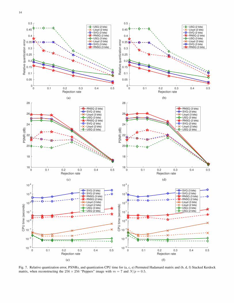
We then compare our proposed RNSQ with SVQ, USQ, and Lloyd’s algorithm, when reconstructing the256×256 “Peppers” image with N/p = 0.5. Figure 7 shows that, for all quantizers, the best reconstructionperformance occurs when some of the measurements are rejected, which matches our expectation, sincea finer grid is put on the remaining measurements after rejection. Furthermore, RNSQ achieves higherPSNRs than other quantizers, for almost all of the test points. This can be explained by the fact thatthe bit assignments in RNSQ provide a better fit to the measurements being quantized. When half ofthe measurements are rejected, all quantizers achieve roughly the same reconstruction performances. Inthis case, the loss of measurements cannot be offset by the improvement of quantization, even after weincrease the bit budget. Furthermore, we observe that RNSQ consumes less CPU time than SVQ, whichimplies that RNSQ has smaller computational complexity.

To test the robustness of RNSQ, we further compare it with other quantization schemes on other256 × 256 images. Table II shows the best PSNRs achieved from different rejection rates, using thestacked Kerdock matrix. Among all methods, RNSQ has the best reconstruction performance for everyimage.

VI. CONCLUSION

Finding computational efficient, and hence scalable, schemes for compressive signal reconstruction fromquantized measurements is a task of vital practical relevance, for example in image reconstruction. We haveproposed an integrated approach which addresses both the choice of sampling scheme and the method ofquantization itself. We have designed fast sampling transforms specially adapted to addressing saturationerror through measurement rejection, and we have proposed a regionalized non-uniform scalar quantizerwhich achieves improved quantization error compared to uniform scalar quantization, while achievingreduced complexity compared to vector quantization. Our experimental results on images demonstrateempirically that our new scheme is scalable and outperforms all state-of-the-art methods.

There remain a number of possible avenues for future work, and we wish to mention two in particular.Firstly, it would be expected that extending RNSQ by performing vector quantization within each regionwould further boost quantization performance. Secondly, an important recent body of research considersmulti-level sampling schemes for image reconstruction with wavelets [19, 20, 21]. Such sampling schemesare inherently non-democratic, and it is a natural question to ask how the quantization schemes we haveproposed in this paper could be combined with multi-level sampling strategies.

14

Rejection rate0 0.1 0.2 0.3 0.4 0.5

Re

lative

qu

an

tiza

tio

n e

rro

r

0

0.05

0.1

0.15

0.2

0.25

0.3

0.35

0.4

0.45

0.5

USQ (2 bits)Lloyd (2 bits)SVQ (2 bits)RNSQ (2 bits)USQ (3 bits)Lloyd (3 bits)SVQ (3 bits)RNSQ (3 bits)

(a)

Rejection rate0 0.1 0.2 0.3 0.4 0.5

Re

lative

qu

an

tiza

tio

n e

rro

r

0

0.05

0.1

0.15

0.2

0.25

0.3

0.35

0.4

0.45

0.5

USQ (2 bits)Lloyd (2 bits)SVQ (2 bits)RNSQ (2 bits)USQ (3 bits)Lloyd (3 bits)SVQ (3 bits)RNSQ (3 bits)

(b)

Rejection rate0 0.1 0.2 0.3 0.4 0.5

PS

NR

(dB

)

16

18

20

22

24

26

28

RNSQ (3 bits)SVQ (3 bits)Lloyd (3 bits)USQ (3 bits)RNSQ (2 bits)SVQ (2 bits)Lloyd (2 bits)USQ (2 bits)

(c)

Rejection rate0 0.1 0.2 0.3 0.4 0.5

PS

NR

(dB

)

16

18

20

22

24

26

28

RNSQ (3 bits)SVQ (3 bits)Lloyd (3 bits)USQ (3 bits)RNSQ (2 bits)SVQ (2 bits)Lloyd (2 bits)USQ (2 bits)

(d)

Rejection rate0 0.1 0.2 0.3 0.4 0.5

CP

U t

ime

(se

co

nd

s)

10 -3

10 -2

10 -1

10 0

10 1

10 2

10 3

10 4

SVQ (3 bits)SVQ (2 bits)RNSQ (3 bits)RNSQ (2 bits)Lloyd (3 bits)Lloyd (2 bits)USQ (3 bits)USQ (2 bits)

(e)

Rejection rate0 0.1 0.2 0.3 0.4 0.5

CP

U t

ime

(se

co

nd

s)

10 -3

10 -2

10 -1

10 0

10 1

10 2

10 3

10 4

SVQ (3 bits)SVQ (2 bits)RNSQ (3 bits)RNSQ (2 bits)Lloyd (3 bits)Lloyd (2 bits)USQ (3 bits)USQ (2 bits)

(f)

Fig. 7. Relative quantization error, PSNRs, and quantization CPU time for (a, c, e) Permuted Hadamard matrix and (b, d, f) Stacked Kerdockmatrix, when reconstructing the 256× 256 “Peppers” image with m = 7 and N/p = 0.5.

15

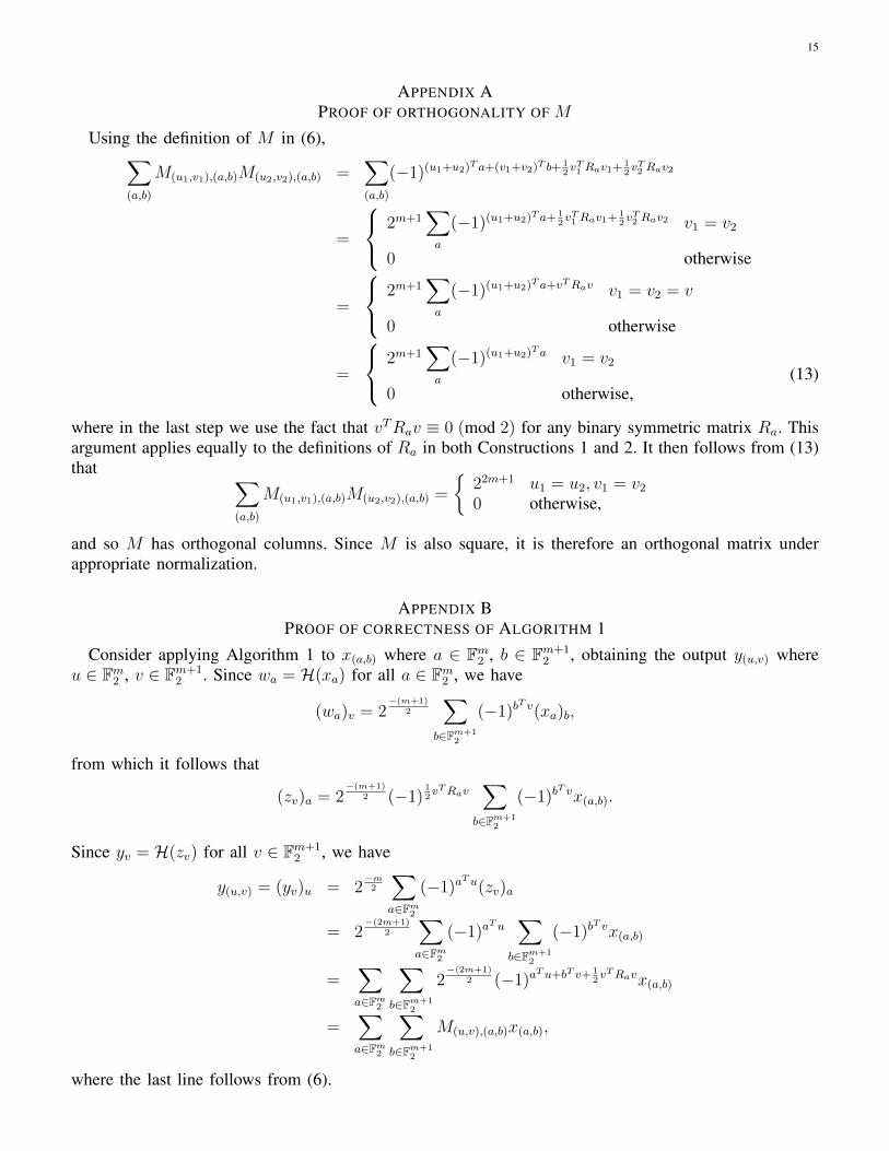
APPENDIX APROOF OF ORTHOGONALITY OF M

Using the definition of M in (6),∑(a,b)

M(u1,v1),(a,b)M(u2,v2),(a,b) =∑(a,b)

(−1)(u1+u2)T a+(v1+v2)T b+ 12vT1 Rav1+ 1

2vT2 Rav2

=

2m+1∑a

(−1)(u1+u2)T a+ 12vT1 Rav1+ 1

2vT2 Rav2 v1 = v2

0 otherwise

=

2m+1∑a

(−1)(u1+u2)T a+vTRav v1 = v2 = v

0 otherwise

=

2m+1∑a

(−1)(u1+u2)T a v1 = v2

0 otherwise,(13)

where in the last step we use the fact that vTRav ≡ 0 (mod 2) for any binary symmetric matrix Ra. Thisargument applies equally to the definitions of Ra in both Constructions 1 and 2. It then follows from (13)that ∑

(a,b)

M(u1,v1),(a,b)M(u2,v2),(a,b) =

22m+1 u1 = u2, v1 = v2

0 otherwise,

and so M has orthogonal columns. Since M is also square, it is therefore an orthogonal matrix underappropriate normalization.

APPENDIX BPROOF OF CORRECTNESS OF ALGORITHM 1

Consider applying Algorithm 1 to x(a,b) where a ∈ Fm2 , b ∈ Fm+12 , obtaining the output y(u,v) where

u ∈ Fm2 , v ∈ Fm+12 . Since wa = H(xa) for all a ∈ Fm2 , we have

(wa)v = 2−(m+1)

2

∑b∈Fm+1

2

(−1)bT v(xa)b,

from which it follows that

(zv)a = 2−(m+1)

2 (−1)12vTRav

∑b∈Fm+1

2

(−1)bT vx(a,b).

Since yv = H(zv) for all v ∈ Fm+12 , we have

y(u,v) = (yv)u = 2−m2

∑a∈Fm2

(−1)aTu(zv)a

= 2−(2m+1)

2

∑a∈Fm2

(−1)aTu

∑b∈Fm+1

2

(−1)bT vx(a,b)

=∑a∈Fm2

∑b∈Fm+1

2

2−(2m+1)

2 (−1)aTu+bT v+ 1

2vTRavx(a,b)

=∑a∈Fm2

∑b∈Fm+1

2

M(u,v),(a,b)x(a,b),

where the last line follows from (6).

16

APPENDIX CDERIVATION OF THE OPTIMAL BIT ASSIGNMENT IN RNSQ

We first write the objective function in (11) as f(α0, α1) = N0 d20 2−2α0 + 4(N11d

211 + N12d

212) 2−2α1 .

Plugging the equality constraint α1 = Nα−η−N0α0

N11+N12into this objective function and setting ∂f

∂α0= 0, we

obtainα?0 =

N −N0

N

[Nα− ηN −N0

+ log2 d0 − 1− 1

2log2

(N11d

211 +N12d

212

N11 +N12

)].

Subsequently, we have

α?1 =N0

N

[Nα− ηN0

+ 1− log2 d0 +1

2log2

(N11d

211 +N12d

212

N11 +N12

)].

To guarantee both α?0 and α?1 are non-negative, we need the parameter constraints in (12).

REFERENCES

[1] E. J. Candes, J. Romberg, and T. Tao, “Robust uncertainty principles: Exact signal reconstructionfrom highly incomplete frequency information,” IEEE Trans. Inf. Theory, vol. 52, no. 2, pp. 489–509,2006.

[2] D. L. Donoho, “Compressed sensing,” IEEE Trans. Inf. Theory, vol. 52, no. 4, pp. 1289–1306, 2006.[3] W. Dai, H. V. Pham, and O. Milenkovic, “Distortion-rate functions for quantized compressive

sensing,” in IEEE Information Theory Workshop on Networking and Information Theory, vol. 61,2009.

[4] A. Zymnis, S. Boyd, and E. J. Candes, “Compressed sensing with quantized measurements,” IEEESignal Process. Lett., vol. 17, no. 2, pp. 149–152, 2010.

[5] J. N. Laska, P. T. Boufounos, M. A. Davenport, and R. G. Baraniuk, “Democracy in action:Quantization, saturation, and compressive sensing,” Applied and Computational Harmonic Analysis,vol. 31, no. 3, pp. 429–443, 2011.

[6] L. Jacques, D. K. Hammond, and J. M. Fadili, “Dequantizing compressed sensing: When oversam-pling and non-gaussian constraints combine,” IEEE Trans. Inf. Theory, vol. 57, no. 1, pp. 559–571,2011.

[7] V. Kostina, M. F. Duarte, S. Jafarpour, and A. R. Calderbank, “The value of redundant measurementin compressed sensing,” in Proc. IEEE Int. Conf. Acoust., Speech, Signal Processing, 2011, pp.3656–3659.

[8] J. Sun and V. Goyal, “Quantization for compressed sensing reconstruction,” in SAMPTA’09, 2009,pp. Special–session.

[9] K. Qiu and A. Dogandzic, “Sparse signal reconstruction from quantized noisy measurements viaGEM hard thresholding,” IEEE Trans. Signal Process., vol. 60, no. 5, pp. 2628–2634, 2012.

[10] U. S. Kamilov, V. K. Goyal, and S. Rangan, “Message-passing de-quantization with applications tocompressed sensing,” IEEE Trans. Signal Process., vol. 60, no. 12, pp. 6270–6281, 2012.

[11] C. Thrampoulidis, E. Abbasi, and B. Hassibi, “The lasso with non-linear measurements is equivalentto one with linear measurements,” in Annual Conference on Neural Information Processing Systems,2015.

[12] A. Gersho and R. M. Gray, Vector quantization and signal compression. Springer Science &Business Media, 2012, vol. 159.

[13] A. R. Calderbank and I. Daubechies, “The pros and cons of democracy,” IEEE Trans. Inf. Theory,vol. 48, no. 6, pp. 1721–1725, 2002.

[14] A. Shirazinia, S. Chatterjee, and M. Skoglund, “Joint source-channel vector quantization forcompressed sensing,” IEEE Trans. Signal Process., vol. 62, no. 14, pp. 3667–3681, 2014.

[15] E. J. Candes and T. Tao, “Decoding by linear programming,” IEEE Trans. Inf. Theory, vol. 51,no. 12, pp. 4203–4215, 2006.

17

[16] D. L. Donoho and M. Elad, “Optimally sparse representation in general (nonorthogonal) dictionariesvia `1 minimization,” Proceedings of the National Academy of Science, vol. 100, no. 5, 2003.

[17] R. Gribonval and M. Nielson, “Sparse representations in unions of bases,” IEEE Trans. Inf. Theory,vol. 49, no. 12, 2003.

[18] S. P. Lloyd, “Least squares quantization in PCM,” IEEE Trans. Inf. Theory, vol. 28, no. 2, pp.129–137, 1982.

[19] J. Romberg, “Imaging via compressive sampling,” IEEE Signal Process. Mag., vol. 25, no. 2, pp.14–20, 2008.

[20] B. Adcock, A. C. Hansen, C. Poon, and B. Roman, “Breaking the coherence barrier: A new theoryfor compressed sensing,” arXiv preprint arXiv:1302.0561, 2013.

[21] F. Krahmer and R. Ward, “Stable and robust sampling strategies for compressive imaging,” IEEETrans. Image Process., vol. 23, no. 2, pp. 612–622, 2014.

[22] S. S. Chen, D. L. Donoho, and M. A. Saunders, “Atomic decomposition by basis pursuit,” SIAMreview, vol. 43, no. 1, pp. 129–159, 2001.

[23] A. R. Calderbank, S. Howard, and S. Jafarpour, “Construction of a large class of deterministic sensingmatrices that satisfy a statistical isometry property,” IEEE J. Sel. Topics Signal Process., vol. 4, no. 2,pp. 358–374, 2010.

[24] M. F. Duarte, S. Jafarpour, and A. R. Calderbank, “Performance of the Delsarte-Goethals frame onclustered sparse vectors,” IEEE Trans. Signal Process., vol. 61, no. 8, pp. 1998–2008, 2013.

[25] H. Monajemi, S. Jafarpour, M. Gavish, and D. L. Donoho, “Deterministic matrices matching thecompressed sensing phase transitions of Gaussian random matrices,” Proceedings of the NationalAcademy of Sciences, vol. 110, no. 4, 2013.

[26] W. Pratt, J. Kane, and H. Andrew, “Hadamard transform image coding,” Proceedings of the IEEE,vol. 57, no. 1, 1969.

[27] T. M. Cover and J. A. Thomas, Elements of Information Theory, 2nd ed. Hoboken, NJ: Wiley,2006.

[28] S. Boyd and L. Vandenberghe, Convex Optimization. Cambridge University Press, 2004.[29] R. Laroia and N. Farvardin, “A structured fixed-rate vector quantizer derived from a variable-length

scalar quantizer. I. memoryless sources,” IEEE Trans. Inf. Theory, vol. 39, no. 3, pp. 851–867, 1993.[30] E. van den Berg and M. P. Friedlander, “Probing the pareto frontier for basis pursuit solutions,”

SIAM Journal on Scientific Computing, vol. 31, no. 2, pp. 890–912, 2008.