1

A subsurface pathway for salinity anomalies propagating from the northwestern 1

subtropical Pacific to the eastern Luzon Strait 2

Youfang Yan1, Eric P. Chassignet2, Yiquan Qi1, Zhichun Zhang1, Kai Yu3, Lingling 3 Liu4 4

1 State Key Laboratory of Tropical Oceanography (South China Sea Institute of 5

Oceanology, Chinese Academy of Sciences), Guangzhou, China 6

2 Center for Ocean-Atmospheric Prediction Studies, Florida State University, 7

Tallahassee, Florida 8

3 Oceanic Modeling and Observation Laboratory, Marine Science College, Nanjing 9

University of Information Science and Technology, Nanjing, China 10

4 Key Laboratory of Ocean Circulation and Waves, Institute of Oceanology, Chinese 11

Academy of Sciences, Qingdao, China 12

13

14

15

16

17

18

19

2

Abstract 20

The subsurface ocean signal propagation from subtropics to tropics has been shown 21

to play a vital role in low-frequency climate variability. In this study, monthly gridded 22

temperature, salinity, and velocity datasets based on Argo profiles, long-term repeat 23

hydrographic observations along 137°E section, and the regional ocean modeling 24

system for 2003-2012 are used to investigate the subduction and propagation of 25

subsurface salinity anomalies along 24.5-25.4kg.m-3 isopycnals in the northwestern 26

Pacific. Both observational and modeling results suggest that the surface salinity 27

anomalies in the northwestern subtropical Pacific (28-35°N, 140-160°E) could be 28

subducted and advected to the eastern Luzon Strait via southwestward thermocline 29

flows. In contrast to salinity anomalies generated in the northeastern subtropical 30

Pacific that propagate slowly and dissipate strongly, these northwestern subtropical 31

Pacific anomalies have a noticeable signature along their propagation pathway and 32

arrive more quickly at the eastern Luzon Strait on time scales of 1-3 years. 33

34

1. Introduction 35

According to the ventilated thermocline theory (Luyten et al. 1983; Woods 1985), 36

surface waters in the mid latitudes could be subducted and transported to the low 37

latitudes via westward and equatorward gyre circulations. Using historical 38

observations, Deser et al. (1996) demonstrated that temperature anomalies in the 39

northeastern subtropical Pacific (NESP) can be subducted and advected equatorward 40

to the tropics along isopycnals. By performing a trajectory analysis of waters in an 41

3

oceanic general circulation model, Gu and Philander (1997) proposed three main 42

pathways for the transport of subtropical waters to the low latitudes: 1) through a 43

zigzag window, waters subducted in the NESP flow equatorward along isopycnals; 2) 44

waters in the central/eastern SP subduct and move westward to the western boundary 45

where they bifurcate, with some of the waters flowing to the tropics through an 46

equatorward western boundary current (WBC); and 3) waters head northward back to 47

the mid latitudes via the poleward WBC, generally taking ~10 years to reach the 48

equator and western boundary and playing an important role in low-frequency climate 49

variability. 50

Salinity ( S ), as a key physical parameter determining density of seawater ( ) 51

especially at mid and high latitudes and as an important marker of ocean circulation 52

and air-sea freshwater, can modulate not only thermal variability but also the 53

hydrologic cycle (e.g., Lukas 2001; Maes et al. 2005; Lagerloef et al. 2010). However, 54

because of the general paucity of salinity observations, especially in the subsurface 55

ocean, few studies have focused on the propagation of salinity in the mid and low 56

latitudes. Taking advantage of recent Argo observations, several studies have 57

investigated the interannual variability of subsurface salinity in the North Pacific (e.g., 58

Sasaki et al. 2010; Ren and Riser 2010; Li et al. 2012a; Yan et al. 2012). Among 59

others, Sasaki et al (2010) reported that anomalous spiciness (potential temperature 60

and salinity variation on isopycnals) generated in the NESP can propagate 61

southwestward to the equator. However, because of the strong dissipation, these 62

anomalies could not reach the western boundary. Using Argo observations, Li et al 63

4

(2012a) and Kolodziejczyk and Gaillard (2012) found a remarkably strong attenuation 64

of spiciness in the NESP along its propagation route, consistent with the results of 65

Sasaki et al. (2010). Alternatively, instead of studying upstream anomalies in the 66

NESP, Yan et al. (2012; 2013) investigated the downstream subsurface salinity 67

anomalies in the eastern Luzon Strait (ELS). They found the anomalies in the ELS are 68

not directly traced back to those in the NESP; instead, they are apparently related to 69

those in the northwestern subtropical Pacific (NWSP). 70

Although the possible connection of the subsurface salinity anomaly between the 71

ELS and the NWSP has been investigated by Yan et al. (2012; 2013), the detailed 72

characterization of this anomaly and its propagation pathway are still not clear. How 73

fast does this anomaly propagate? Does it extend to the low latitude regions? These 74

questions will be addressed in the present study. The remainder of the paper is 75

organized as follows: A brief description of the data and method of analysis are 76

presented in section 2; the subduction and propagation pathways of salinity anomalies 77

in the northwestern Pacific are explained in section 3; and results are summarized and 78

discussed in section 4. 79

2. Data and method of analysis 80

The monthly mean 1°×1° temperature and salinity fields compiled by Hosoda et al. 81

(2008), known as the Grid Point Values of the Monthly Objective Analysis (MOAA 82

GPV) based mainly on Argo observations for the period 2003-2012, are used in this 83

study. In situ measurements by conductivity-temperature depth along 137°E sections 84

provided by the Japan Meteorological Agency (JMA) are also used. In order to study 85

5

salinity propagation pathways, 2003-2012 velocity model outputs were used from the 86

Regional Ocean Modeling System (ROMS) with 1/8º horizontal resolution from 45°S 87

to 65°N and from 99°E to 70°W, and 30 levels in the vertical. For a detailed 88

description and validation of ROMS with in situ observations, the reader is referred to 89

Zhang et al. (2015, personal communication). The evaporation (E) from the 90

Objectively Analyzed air-sea Fluxes (OAFlux) project was provided by the Woods 91

Hole Oceanographic Institution (Yu and Weller 2007) while the precipitation (P) 92

fields come from the Global Precipitation Climatology Project (GPCP). Finally, wind 93

stresses from the Cross-Calibrated Multi-Platform (CCMP) are used, as are sea 94

surface geostrophic velocity anomalies provided by Archiving, Validation and 95

Interpretation of Satellite Oceanographic (AVISO) on a 0.25°×0.25°. 96

The Montgomery geostrophic streamfunction (Montgomery 1937) is defined by 97

00

ˆ ˆ(P P ) (S[p ], [p ]),p )dPP

P (1) 98

Where P is the reference pressure, 0P is the sea surface pressure, ̂ is the specific 99

volume anomaly. The mean surface geostrophic velocities are derived from the 100

MDT_CNES-CLS09 product (Rio et al. 2011). The statistical analysis of interannual 101

salinity patterns on the given isopycnal surface is performed with the Extended 102

Empirical Orthogonal Function (EEOF). Compared to the classical EOF analysis, the 103

EEOF analysis can catch the propagating pattern by introducing time lag into the 104

covariance matrix. The annual subduction rate annR , which is calculated by tracing 105

water parcels released at the base of the winter mixed layer for one year in a 106

Lagrangian framework, is expressed as (Huang and Qiu 1998): 107

6

2

1m 2 m 1

1 1[ ( ) ( )]

t

ann mbt

R w dt h t h tT T

, (2) 108

where T represents the time period of integration; 1t and 2t are the end of the first 109

and second winter, respectively; mh is the winter mixed layer depth (MLD); and 110

mbw is the vertical velocity at the base of the mixed layer. 111

3. Isopycnal salinity anomalies and their propagation in the northwestern 112

subtropical Pacific (NWSP) 113

3.1 Salinity anomalies 114

The recent availability of Argo observations has led to the study of isopycnal 115

salinity anomalies in the NWSP (Li et al. 2012a; Yan et al. 2012; 2013; Sugimoto et al. 116

2013). Because maximum subduction occurs in the winter, we first show in Fig.1b the 117

standard deviation of winter salinity anomalies averaged on the 24.5-25.4kg.m-3 118

isopycnals, where the water exhibits a sustained freshening trend (Yan et al. 2012; 119

2013; Nan et al. 2015). There is a band of large salinity variability in the Kuroshio 120

Extension, with magnitude up to 0.1 PSU. This anomaly compares favorably with that 121

of Yan et al. (2013) and Nan et al. (2015), and spreads along the 24.5-25.4kg.m-3 122

outcrop lines (Fig.1c). 123

The salinity distribution is generally the result of a balance between surface 124

freshwater fluxes (precipitation P, evaporation E) and ocean dynamics. As shown in 125

Fig. 1a, the standard deviation of E-P attains its maximum at the northern rims of 126

subtropical gyre (35°N), located slightly northwestward of the area of maximum 127

salinity variability, most notably in the southeastern side of study region. This 128

displacement suggests the potential impact of ocean dynamics on salinity variability. 129

A careful examination of surface wind stress indicates that a strong northwesterly 130

7

wind prevails in the maximum variability of the E-P region (Fig. 1a). The 131

northwesterly wind drives a positive salinity advection toward the salinity maximum 132

variability region, thus leading to a southeastward shift of salinity maximum to the 133

region of maximum E-P variability. In addition, the maximum salinity variability is 134

found in the regions where the vertical Ekman pumping is predominantly downward 135

(Fig.1a). The downward Ekman pumping provides a favorable condition for the 136

subduction of high-variability surface waters into the ocean interior, although the 137

lateral induction becomes dominant as a result of large winter mixed layer depth 138

(MLD) gradients (Fig. 1c) in the studied region (Suga et al. 2008). 139

By transferring the waters from the mixed layer into the ocean interior, subduction 140

is another kinematical and dynamical process coupling the atmosphere and the 141

subsurface ocean. Before proceeding to calculate the subduction rate in the NWSP, we 142

first examine the MLD. As shown in Fig. 1c, the winter MLD is generally shallow 143

(~50 m) in the low latitudes and gradually becomes deeper toward the higher latitudes, 144

with a maximum lying around the southern edge of maximum salinity variability. This 145

maximum MLD allows winter mixed layer waters to subduct into the thermocline 146

(Qiu and Huang 1995). The annual subduction rate, which is calculated using the 147

Argo temperature and salinity data combined with the NCEP wind field, is shown in 148

Fig.1d. It is worth noting that the regions of largest annual subduction rate have been 149

found to be at the southern edge of the highest salinity variability and maximum MLD 150

region (Fig.1b, 1c and 1d), reflecting the dominant contribution of lateral induction in 151

the salinity subduction, consistent with Qiu and Huang (1995) and Suga et al. (2008). 152

8

To demonstrate the horizontal transport of the subducted salinity anomalies in the 153

thermocline, we release passive particles at the base of the mixed layer in February 154

and advect them with the flow field for one year. The trajectories of the passive 155

particles (Fig. 1d) match well with the streamlines of Montgomery geostrophic flow 156

on 24.5-25.4 kg.m-3 isopycnals, suggesting the subducted salinity anomalies in the 157

outcropping regions (Fig.1e-1f) may be transferred to the western tropical Pacific by a 158

southwestward horizontal flow. 159

3.2 Propagation pathway 160

To illustrate where and when the salinity anomalies propagate, the EEOF 161

decomposition from a statistical perspective is first applied with time lags of 1, 3, 5, 7, 162

9, 11, and 13 months, respectively. The spatial pattern of the first mode (EEOF1), with 163

time lags of 1 month and accounting for ~70.1% of the total variance and explaining a 164

significant part of salinity variability, and the corresponding time coefficients are 165

illustrated in Fig. 2a and 2b. The first mode shows a marked freshening of waters in 166

the NWSP with salinity decreasing during 2003-12, consistent with the results of 167

Fig.1e-1f and those of Sugimoto et al. (2013) and Nan et al. (2015). The strongest 168

freshening trend occurs in the surface layer (-0.2psu/10yr) near 30°N and decreases 169

against depth. It should also be noted that the salinity anomalies south of 15°N are 170

entirely out of phase with those north of 15°N, displaying a dipolar structure. This 171

dipolar structure is also found in the trends of salinity anomalies based on Argo 172

observations and the repeated oceanographic observation section along 137°E (Fig. 3). 173

The dissimilar trends in the north and south of 15°N indicate that the mechanisms 174

9

controlling the salinity in these two regions are quite different. The reason for this 175

difference is unclear and is beyond the scope of this study. To illustrate the 176

propagation pathway of salinity anomalies north of 15°N, the contour lines of -0.15 177

PSU with time lags of 1, 3, 5, 7, 9, 11, and 13 months based on EEOF are shown (Fig. 178

2a). We observe that a negative anomaly emerges and propagates southwestward from 179

the region south of the Kuroshio Extension toward the western boundary, taking about 180

13 months to reach the ELS (see the label number of contours). This propagation time 181

is consistent with the results of Oka [2009], Oka and Qiu [2012] and Qiu and Chen 182

[2013]. Consistent with the results of Nan et al. (2015), the southwestward 183

propagation of the signal corresponds well with the Pacific Decadal Oscillation (PDO) 184

(r=-0.68), which is significantly different from zero at the 95% confidence level 185

(r=-0.596) according to a Student’s t test. Compared to the PDO index, the correlation 186

(r=-0.60) between the anomalies and the Nino3.4 index is lower and possibly 187

insignificant during 2003-2012. 188

To further document the propagation pathway, we now focus on the latitude-time 189

diagram of salinity anomalies averaged vertically over the 24.5-25.4kg.m-3 isopycnals 190

along the Montgomery geostrophic streamlines between 28.0 and 29.0m2/s2 (Fig. 2d). 191

The latitude-time diagram of salinity anomalies indicates that the propagated salinity 192

signals exhibit decadal timescale variability and experience two major phase-flipping 193

events in 2005 and 2009. In order to determine what causes these subsurface salinity 194

changes, we look at the surface salinity anomalies averaged over the subduction 195

region (28°-35°N, 140°-160°E). Two extreme opposing phases of the surface salinity 196

10

anomalies are found in 2004-2006 and 2009-2011, consistent with the mixed layer 197

salinity variability in the subtropical mode water formation region (Sugimoto et al. 198

2013). The timing of these peaks nearly coincides with that of the subsurface salinity 199

anomalies, suggesting that the propagation of salinity anomalies along the isopycnals 200

mainly comes from the surface in the outcrop zones. 201

To view the full cycle of salinity anomalies propagation in the NWSP, in Fig. 4 we 202

plot the monthly maps of positive salinity anomalies averaged over 24.5-25.4kg.m-3 203

isopycnals during 2005-2006, corresponding to the strongest salinity anomalies as 204

shown in Fig. 2d. This reveals that the anomaly is first detected at 25°-35°N in Feb 205

2005 (Fig. 3a); it then migrates southwestward along the contours of the Montgomery 206

geostrophic streamfunction and approaches the ELS in Jan 2006 (Fig. 3l). The path of 207

this anomaly is consistent with the results of EEOF (Fig. 2a), suggesting that the 208

surface salinity anomalies in the northwest subtropical outcropping region may 209

propagate to the ELS via the southwestward subtropical gyre circulations. 210

Previous studies (Parr 1938; Montgomery 1938) have demonstrated that salinity is 211

also a useful dynamical tracer conservatively following parcels' trajectory along 212

isopycnal surfaces. Thus, here we performed forward Lagrangian particle tracing 213

experiments based on every three days velocity of ROMS for 2003-2012 in order to 214

independently identify the propagation path of the subsurface salinity anomalies in the 215

subtropical gyre. The trajectories of these particles are shown in Fig. 5. All the 216

particles can be traced to the ELS by southward subtropical gyre circulations, with 217

tracing periods ranging from 1-3 years. The particles released in the western higher 218

11

salinity trend subduction areas (see Fig. 3a) can be traced to the ELS faster (~1yr) 219

than those released in the lower salinity trend eastern areas (~3yrs). In addition, the 220

tracing period is not qualitatively sensitive to positive or negative salinity anomalies 221

(Fig. 5b and Fig. 5c), which suggests that salinity variations in the ELS can be 222

influenced by upstream salinity variations through southwestward subtropical gyre 223

circulations. 224

4. Summary and discussion 225

This study provides a detailed description of the subduction and propagation of 226

subsurface salinity anomalies in the northwest Pacific using the temperature, salinity, 227

and velocity data provided mainly by Argo observations, in situ observations, and 228

ROMS. Tracing of the subsurface salinity anomalies was accomplished by conducting 229

an EEOF analysis, examining the extreme salinity anomalies along 24.5-25.4kg.m-3 230

isopycnals, and eventually designing forward Lagrangian particle tracing experiments. 231

As a result, we found that salinity anomalies generated in the northwest Pacific 232

subduction region (28°-35°N, 140°-160°E) can be subducted and can propagate to the 233

ELS via southwestward subtropical gyre circulations on time scales of 1 to 3years. 234

The possible connection between the mid latitudes and the western boundary via 235

the subsurface salinity propagation in the North Pacific has been recently examined; 236

however because of strong dissipation, the salinity anomalies originating in the NESP 237

nearly vanished before reaching the western boundary (e.g., Li et al. 2012b; 238

Kolodziejczyk and Gaillard 2012). In this study, we show that the anomalies 239

generated in the NWSP outcropping region (28°-35°N, 140°-160°E) are strong and 240

12

they reach the ELS on time scales of 1 to 3 years. 241

Although the propagation pathway and timing of salinity anomalies between the 242

mid latitudes and the ELS is addressed in this study, several open questions still 243

remain. What mechanism controls the generation and subduction of salinity anomalies 244

in the outcrop region? How do the salinity anomalies affect its downstream western 245

Pacific warm pool change? A recent study has suggested that the warm pool change is 246

related not only to the large-scale air-sea processes, but also to the subsurface ocean 247

processes (Qu et al. 2013). Knowledge of the subsurface salinity change and its 248

linkage with the warm pool’s thermocline structure would provide a crucial basis for 249

understanding of ocean-atmosphere interaction and the climate effects of subducted 250

salinity anomalies. 251

Acknowledgments 252

This study was supported by the National Basic Research Program of China 253

(2013CB430301), the Strategic Priority Research Program of the Chinese Academy of 254

Sciences (XDA11010203), and the National Natural Science Foundation of China 255

(41276025). 256

257

References 258

Deser, C., M. A. Alexander, and M. S. Timlin, 1996: Upper-ocean thermal variations 259

in the North Pacific during 1970-1991, J. Clim., 9, 1840-1855. 260

Gu, D., and G. S. Philander, 1997: Interdecadal climate fluctuations that depend on 261

exchanges between the tropics and extratropics, Science, 275, 805-807. 262

Hosoda, S., T. Ohira, and T. Nakamura, 2008: A monthly mean dataset of global 263

oceanic temperature and salinity derived from Argo float observations, JAMSTEC 264

Report of Research and Development, 8, 47-59. 265

13

Huang, R. X., and B. Qiu, 1998: The structure of the wind-driven circulation in the 266

subtropical South Pacific Ocean, J. Phys. Oceanogr., 28, 1173-1186. 267

Huang, B., and Z. Liu, 1999: Pacific subtropical-tropical thermocline water exchange 268

in the National Centers for Environmental Prediction ocean model, J. Geophys. 269

Res., 104, 11065-11076. 270

Kolodziejczyk, N., and F. Gaillard, 2012: Observation of spiciness interannual 271

variability in the Pacific pycnocline, J. Geophys. Res., 117, C12018, doi: 272

10.1029/2012JC008365. 273

Lagerloef, G., R. Schmitt, J. Schanze, and H. Y. Kao, 2010: The Ocean and the global 274

water cycle, Oceanography, 23(4), 82-93. 275

Li, Y. L., F. Wang, and F. G. Zhai, 2012a: Interannual variations of subsurface 276

spiciness in the Philippine Sea: Observations and mechanism, J. Phys. Oceanogr., 277

42, 1022-1038. 278

Li, Y., F. Wang, and Y. Sun, 2012b: Low-frequency spiciness variations in the 279

tropical Pacific Ocean observed during 2003-2012, Geophys. Res. Lett., 39, L23601, 280

doi: 10.1029/2012GL053971. 281

Luyten, J., J. Pedlosky, and H. M. Stommel, 1983: The ventilated thermocline, J. Phys. 282

Oceanogr., 13, 292-309. 283

Lukas, R., 2001: Freshening of the upper thermocline in the North Pacific subtropical 284

gyre associated with decadal changes of rainfall, Geophys. Res. Lett., 28, 285

3485-3488. 286

Maes, C., J. Picaut, and S. Belamari, 2005: Importance of the salinity barrier layer for 287

the buildup of El Nino, J. Clim., 18, 104-118. 288

Montgomery, R. B., 1937: A suggested method for representing gradient flow in 289

isentropic surfaces, Bull. Amer. Meteor. Soc. 18, 210-212. 290

Montgomery, R. B., 1938: Circulation in upper layers of southern North Altantic 291

deduced with use of isentropic analysis, Pap. Phys. Oceanogr., 6, 1-55. 292

Nan, F., F. Yu, H. Xue, R. Wang, and G. Si, 2015: Ocean salinity changes in the 293

northwest Pacific subtropical gyre: the quasi-decadal oscillation and the freshening 294

trend, J. Geophys. Res.Oceans, 120, doi: 10.1002/2014JC010536. 295

14

Oka, E., 2009: Seasonal and interannual variation of North Pacific subtropical mode 296

water in 2003-2006, J. Oceanogr., 65,151-164. 297

Oka, E., and B. Qiu, 2012: Progress of North Pacific mode water research in the past 298

decade, J. Oceanogr., 68, 5-20. 299

Parr, A. E., 1938: Isopycnic analysis of current flow by means of identifying 300

properties, J. Mar. Res., 1, 133-154. 301

Qiu, B., and R. X. Huang, 1995: Ventilation of the North Atlantic and North Pacific: 302

Subduction versus obduction, J. Phys. Oceanogr., 25, 2374-2390. 303

Qiu, B., and S. Chen, 2013: Concurrent decadal mesoscale eddy modulations in the 304

Western North Pacific subtropical Gyre, J. Phys. Oceanogr., 43, 344-358. 305

Qu, T. D, S. Gao, R. A. Fine, 2013: Subduction of South Pacific Tropical Water and 306

Its Equatorward Pathways as Shown by a Simulated Passive Tracer, J. Phys. 307

Oceanogr., 43, 1551-1565. 308

Ren, L., and S. C. Riser, 2010: Observations of decadal time scale salinity changes in 309

the subtropical thermocline of the North Pacific Ocean, Deep-Sea Research, 57, 310

1161-1170. 311

Rio, M. H., S. Guinehut, and G. Larnicol, 2011: New CNES-CLS09 global mean 312

dynamic topography computed from the combination of GRACE data, altimetry, 313

and in situ measurements, J. Geophys. Res., 116, doi: 10.1029/2010JC006505. 314

Sasaki, Y. N., N. Schneider, N. Maximenko, and K. Lebedev, 2010: Observational 315

evidence for propagation of decadal spiciness anomalies in the North Pacific, 316

Geophys. Res. Lett., 37, L07708, doi: 07710.01029/02010GL042716. 317

Toshio Suga,Yoshikazu Aoki, Hiroko Saito, Kimio Hanawa, 2008:Ventilation of the 318

North Pacific subtropical pycnocline and mode water formation, Progress in 319

Oceanography, 77, 285-297. 320

Sugimoto, S., N. Takahashi, and K. Hanawa, 2013: Marked freshening of North 321

Pacific subtropical mode water in 2009 and 2010: Influence of freshwater supply in 322

the 2008 warm season, Geophys. Res. Lett., 40, 3102-3105. 323

Woods, J. D., 1985: Physics of thermocline ventilation, In Coupled 324

Atmosphere-Ocean Models, ed. by J. C. J. Nihoul. 325

15

Yan, Y., D. Xu, Y. Qi, and Z. Gan, 2012: Observations of freshening in the northwest 326

Pacific subtropical Gyre near Luzon Strait, Atmosphere-Ocean, doi: 327

10.1080/07055900.07052 012.07715078. 328

Yan, Y., E. P. Chassignet, Y. Qi, and W. K. Dewar, 2013: Freshening of Subsurface 329

Waters in the Northwest Pacific Subtropical Gyre: Observations and Dynamics, J. 330

Phys. Oceanogr., 43, 2733-2750. 331

Yu, L., X. Jin, and R. A. Weller, 2008: Multidecade Global Flux Datasets from the 332

Objectively Analyzed Air-sea Fluxes (OAFlux) Project: Latent and sensible heat 333

fluxes, ocean evaporation, and related surface meteorological variables. Woods 334

Hole Oceanographic Institution, OAFlux Project Technical Report. OA-2008-01, 335

64pp. Woods Hole. Massachuse. 336

Zhichun ZHANG, Huijie XUE, Fei Chai, Yi Chao, 2015: Inter-annual Variability of 337

the North Equatorial Current Based on Model Results, Under Reviewed. 338

Figures

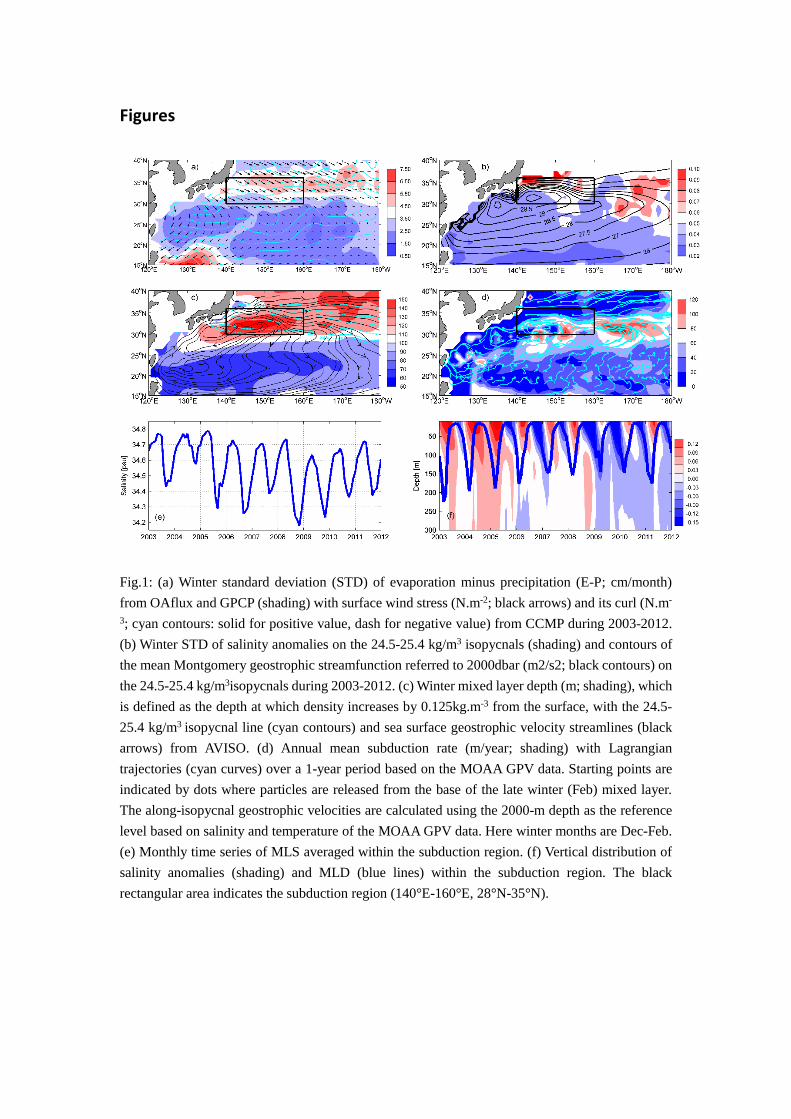
Fig.1: (a) Winter standard deviation (STD) of evaporation minus precipitation (E-P; cm/month) from OAflux and GPCP (shading) with surface wind stress (N.m-2; black arrows) and its curl (N.m-

3; cyan contours: solid for positive value, dash for negative value) from CCMP during 2003-2012. (b) Winter STD of salinity anomalies on the 24.5-25.4 kg/m3 isopycnals (shading) and contours of the mean Montgomery geostrophic streamfunction referred to 2000dbar (m2/s2; black contours) on the 24.5-25.4 kg/m3isopycnals during 2003-2012. (c) Winter mixed layer depth (m; shading), which is defined as the depth at which density increases by 0.125kg.m-3 from the surface, with the 24.5-25.4 kg/m3 isopycnal line (cyan contours) and sea surface geostrophic velocity streamlines (black arrows) from AVISO. (d) Annual mean subduction rate (m/year; shading) with Lagrangian trajectories (cyan curves) over a 1-year period based on the MOAA GPV data. Starting points are indicated by dots where particles are released from the base of the late winter (Feb) mixed layer. The along-isopycnal geostrophic velocities are calculated using the 2000-m depth as the reference level based on salinity and temperature of the MOAA GPV data. Here winter months are Dec-Feb. (e) Monthly time series of MLS averaged within the subduction region. (f) Vertical distribution of salinity anomalies (shading) and MLD (blue lines) within the subduction region. The black rectangular area indicates the subduction region (140°E-160°E, 28°N-35°N).

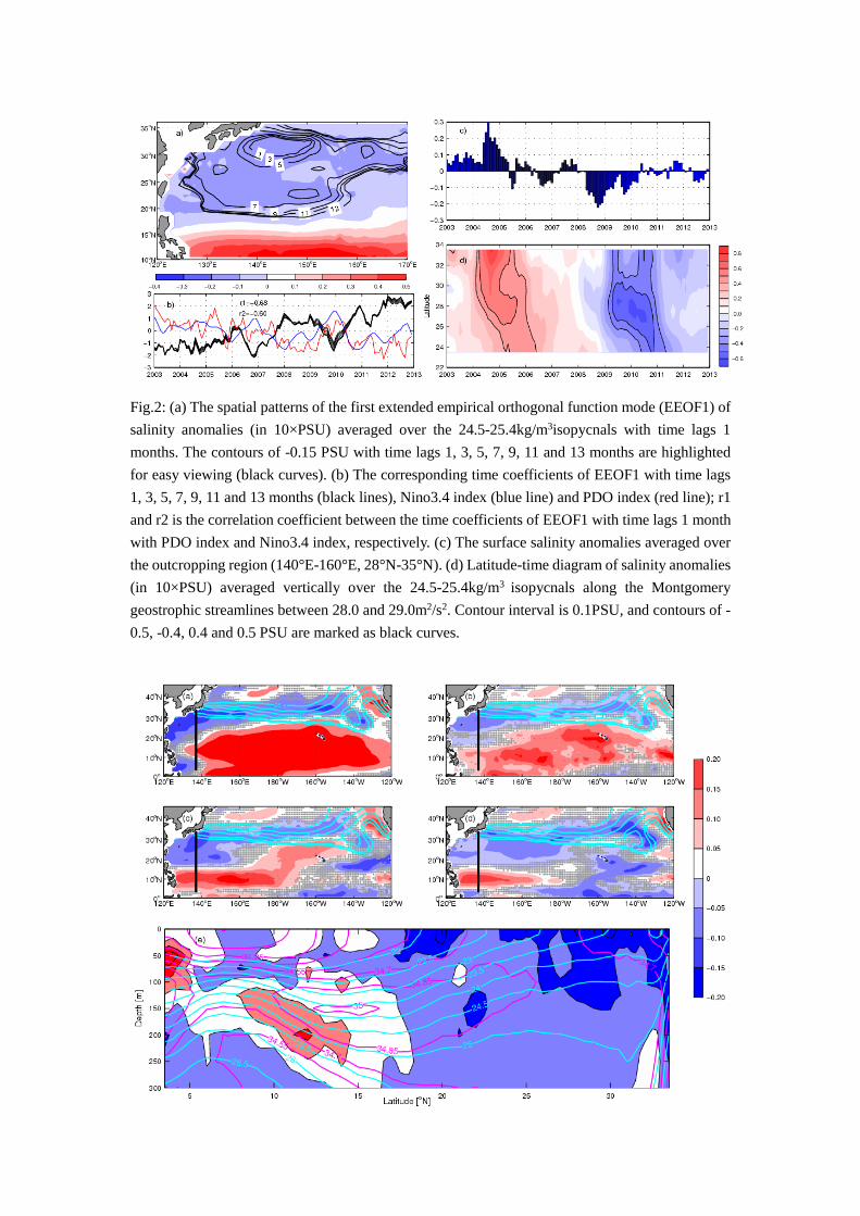
Fig.2: (a) The spatial patterns of the first extended empirical orthogonal function mode (EEOF1) of salinity anomalies (in 10×PSU) averaged over the 24.5-25.4kg/m3isopycnals with time lags 1 months. The contours of -0.15 PSU with time lags 1, 3, 5, 7, 9, 11 and 13 months are highlighted for easy viewing (black curves). (b) The corresponding time coefficients of EEOF1 with time lags 1, 3, 5, 7, 9, 11 and 13 months (black lines), Nino3.4 index (blue line) and PDO index (red line); r1 and r2 is the correlation coefficient between the time coefficients of EEOF1 with time lags 1 month with PDO index and Nino3.4 index, respectively. (c) The surface salinity anomalies averaged over the outcropping region (140°E-160°E, 28°N-35°N). (d) Latitude-time diagram of salinity anomalies (in 10×PSU) averaged vertically over the 24.5-25.4kg/m3 isopycnals along the Montgomery geostrophic streamlines between 28.0 and 29.0m2/s2. Contour interval is 0.1PSU, and contours of -0.5, -0.4, 0.4 and 0.5 PSU are marked as black curves.

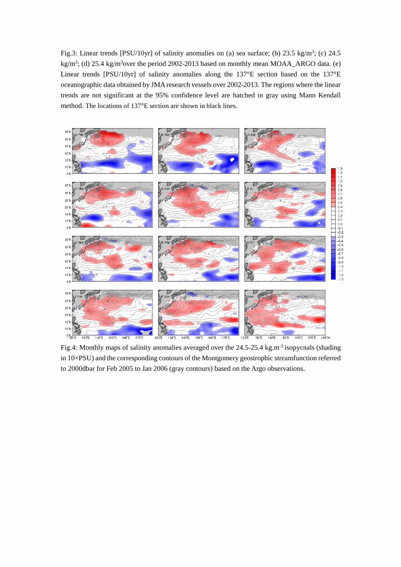
Fig.3: Linear trends [PSU/10yr] of salinity anomalies on (a) sea surface; (b) 23.5 kg/m3; (c) 24.5 kg/m3; (d) 25.4 kg/m3over the period 2002-2013 based on monthly mean MOAA_ARGO data. (e) Linear trends [PSU/10yr] of salinity anomalies along the 137°E section based on the 137°E oceanographic data obtained by JMA research vessels over 2002-2013. The regions where the linear trends are not significant at the 95% confidence level are hatched in gray using Mann Kendall method. The locations of 137°E section are shown in black lines.

Fig.4: Monthly maps of salinity anomalies averaged over the 24.5-25.4 kg.m-3 isopycnals (shading in 10×PSU) and the corresponding contours of the Montgomery geostrophic streamfunction referred to 2000dbar for Feb 2005 to Jan 2006 (gray contours) based on the Argo observations.

Fig.5: Trajectories of the forward Lagrangian particle tracing of the salinity anomaly signals based on the velocity mean vertically averaged between the potential density of 24.5 and 25.4 kg/m3(vector; m/s) for a) 2003-2012; b) 2004-2006; c) 2009-2011. Red circles indicate the starting locations, the red rectangles indicate the positions of the signals propagate for one year, the black rectangular area indicates the subduction region (140°E-160°E, 28°N-35°N).