1 A New Chase-type Soft-decision Decoding Algorithm for

arX

iv:1

309.

1555

v3 [

cs.IT

] 4

Dec

201

31

A New Chase-type Soft-decision Decoding

Algorithm for Reed-Solomon Codes

Siyun Tang and Xiao MaMember, IEEE

Abstract

This paper addresses three relevant issues arising in designing Chase-type algorithms for Reed-

Solomon codes: 1) how to choose the set of testing patterns; 2) given the set of testing patterns, what

is the optimal testing order in the sense that the most-likely codeword is expected to appear earlier;

and 3) how to identify the most-likely codeword. A new Chase-type soft-decision decoding algorithm is

proposed, referred to astree-based Chase-type algorithm. The proposed tree-based Chase-type algorithm

takes the set of all vectors as the set of testing patterns, and hence definitely delivers the most-likely

codeword provided that the computational resources are allowed. All the testing patterns are arranged in

an ordered rooted tree according to the likelihood bounds ofthe possibly generated codewords. While

performing the algorithm, the ordered rooted tree is constructed progressively by adding at most two

leafs at each trial. The ordered tree naturally induces a sufficient condition for the most-likely codeword.

That is, whenever the tree-based Chase-type algorithm exits before a preset maximum number of trials is

reached, the output codeword must be the most-likely one. When the tree-based Chase-type algorithm

is combined with Guruswami-Sudan (GS) algorithm, each trial can be implement in an extremely

simple way by removing from the gradually updated Grobner basis one old point and interpolating one

new point. Simulation results show that the tree-based Chase-type algorithm performs better than the

recently proposed Chase-type algorithm by Bellorado et al with less trials (on average) given that the

maximum number of trials is the same. Also proposed are simulation-based performance bounds on the

maximum-likelihood decoding (MLD) algorithm, which are utilized to illustrate the near-optimality of

the tree-based Chase-type algorithm in the high signal-to-noise ratio (SNR) region. In addition, the tree-

based Chase-type algorithm admits decoding with a likelihood threshold, that searches the most-likely

codeword within an Euclidean sphere rather than a Hamming sphere.

This work is supported by the 973 Program (No.2012CB316100)and the NSF (No.61172082) of China.The authors are with the Department of Electronics and Communication Engineering, Sun Yat-sen University, Guangzhou

510006, China (Emails: [email protected], [email protected]).

http://arxiv.org/abs/1309.1555v3

2

Index Terms

Chase-type algorithm, flipping patterns, Guruswami-Sudanalgorithm, hard-decision deocoding,

Reed-Solomon codes, soft-decision decoding, testing patterns.

I. INTRODUCTION

Reed-Solomon (RS) codes are an important class of algebraiccodes, which have been widely

used in many practical systems, including space and satellite communications, data storage,

digital audio/video transmission and file transfer [1]. Thewidespread use of RS codes is pri-

marily due to their large error-correction capability, a consequence of their maximum distance

separable (MDS) property. Investigating the decoding algorithms for RS codes is important both

in practice and in theory. The traditional hard-decision decoding (HDD) algorithms, such as

Berlekamp-Massey (BM) [2], Welch-Berlekamp (WB) [3] and Euclidean [4] algorithms, are

efficient to find the unique codeword (if exists) within a Hamming sphere of radius less than the

half minimum Hamming distance. Hence, their error-correction capability is limited by the half

minimum Hamming distance bound. In contrast, Guruswami-Sudan (GS) algorithm [5] [6] can

enlarge the decoding radius and may output a list of candidate codewords. Hence, GS algorithm

can correct errors beyond the half minimum Hamming distancebound. To further improve the

performance, one needs turn to the soft-decision decoding (SDD) algorithms.

The soft-decision decoding (SDD) algorithms can be roughlydistinguished into two classes.

One is the algebraic soft-decision decoding algorithm as proposed by Koetter and Vardy [7].

The Koetter-Vardy (KV) algorithm transforms the soft information into the multiplicity matrix

that is then taken as input to the GS algorithm. The KV algorithm outperforms the GS algorithm

but suffers from high complexity. To reduce the complexity,a progressive list-enlarged algebraic

soft decoding algorithm has been proposed in [8][9]. The other class of SDD algorithms are

based on multiple trials, where some known decoding algorithm is implemented for each trial.

The first algorithm of this type could be the so-called generalized minimum distance (GMD)

decoding algorithm [10], which repeatedly implements an erasure-and-error decoding algorithm

while successively erasing an even number of the least reliable positions (LRPs). The GMD

decoding algorithms can be enhanced as presented in [11][12]. In [13], three other soft-decision

decoding algorithms were presented, now referred to as Chase-1, Chase-2, and Chase-3, as

distinguished from the set of testing patterns. At each trial, the Chase algorithm implements the

3

traditional HDD for each testing pattern from a pre-determined set. To improve the performance,

one can either enlarge the set of testing patterns (say the Chase-GMD decoding algorithm [14])

or implement a more powerful decoding algorithm (say the Chase-KV decoding algorithm [15])

for each trial. Other soft-decision decoding algorithms based on multiple trials can be found

in [16] and [17]. In [16], re-encoding is performed for each trial, where the generator matrix is

adapted based on most reliable positions (MRPs) specified bythe ordered statistics. In [17] [18],

a decoding algorithm combined with belief propagation is performed for each trial, where the

parity-check matrix is iteratively adapted based on the LRPs.

In this paper, we focus on the Chase-type decoding algorithm. Let Cq[n, k] be an RS code

over the finite field of sizeq with lengthn, dimensionk, and the minimum Hamming distance

dmin = n−k+1, Generally, a Chase-type soft-decision decoding algorithm has three ingredients:

1) a set offlipping patternsF∆= {f(0), · · · , f(L−1)} wheref(ℓ) is a vector of lengthn, 2) a hard-

decision decoder (HDD), and 3) a stopping criterion. Given these three ingredients, a Chase-

type decoding algorithm works as follows. For eachℓ ≥ 0, the Chase-type algorithm makes

a trial by decodingz − f(ℓ) with the HDD. If the HDD is successful, the output is referredto

as a candidate codeword. Once some candidate is found to satisfy the stopping criterion, the

algorithm terminates. Otherwise, the algorithm chooses asoutput the most likely candidate after

all flipping patterns inF are tested.

The commonly-usedF is constructed combinatorially. For example, the Chase-2 algorithm [13],

which was originally proposed for binary codes, finds thetmin∆= ⌊(dmin− 1)/2⌋ LRPs and then

constructs2tmin flipping patterns. Obviously, the straightforward generalization of Chase-2 from

binary to nonbinary incurs high complexity especially for largeq anddmin. To circumvent this,

the low-complexity Chase (LCC) decoding algorithm [19] forRS codes constructs2η flipping

patterns by first findingη LRPs and then restricts only two most likely symbols at each LRP.

For the HDD algorithm required in the Chase-type algorithm,one usually chooses the traditional

HDD algorithm. In contrast, the LCC algorithm implements the GS decoding algorithm (with

multiplicity one) for each trial. This algorithm has a clearadvantage when two flipping patterns

diverge in only one coordinate, in which case backward interpolation architecture [20] can be

employed to further reduce the decoding complexity. For thestopping criterion, some authors use

the genie-aided rule[17], which terminates the algorithm whenever the transmitted codeword is

found. This criterion is impractical but meaningful to accelerate the simulation and to provide a

4

lower bound on the decoding error probability. In [21], the authors provide a sufficient condition

for optimality, which can be used to terminate the Chase-type algorithm before all flipping

patterns are tested.

The main objective of this paper is to address the following three relevant issues: 1) how

to choose the set of flipping patterns; 2) given the set of flipping patterns, what is the optimal

testing order in the sense that the most-likely codeword is expected to appear earlier; and 3) how

to identify the most-likely codeword.

We propose to arrange all possible flipping patterns into an ordered rooted tree, which is

constructed progressively by adding at most two leafs at each trial. The ordered tree naturally

induces a sufficient condition for the most-likely codeword. That is, whenever thetree-based

Chase-type algorithmexits before a preset maximum number of trials is reached, the output

codeword must be the most-likely one. In addition, when the new algorithm is combined with

the GS algorithm, each trial can be implement in an extremelysimple way by removing from

the gradually updated Grobner basis one old point and interpolating one new point. Simulation

results show that the proposed algorithm performs better than the LCC algorithm [19] with less

trials (on average) given that the maximum number of trials is the same. To illustrate the near-

optimality of the proposed algorithm in the high signal-to-noise ratio (SNR) region, we also

propose a method to simulate performance bounds on the maximum-likelihood decoding (MLD)

algorithm. Moreover, the proposed algorithm admits decoding with a likelihood threshold, that

searches the most-likely codeword within an Euclidean sphere rather than a Hamming sphere.

The rest of this paper is organized as follows. Sec. II definesthe ordered rooted tree of flipping

patterns and provides a general framework of the tree-basedChase-type algorithm. In Sec. III,

the tree-based Chase-type algorithm is combined with the GSalgorithm. Numerical results and

further discussion are presented in Sec. IV. Sec. V concludes this paper.

II. TESTING ORDER OFFLIPPING PATTERNS

A. Basics of RS Codes

Let Fq∆= {α0, α1, · · · , αq−1} be the finite field of sizeq. A codeword of the RS codeCq[n, k]

can be obtained by evaluating a polynomial of degree less than k overn distinct points, denoted

by L∆= {β0, β1, · · · , βn−1} ⊆ Fq. To be precise, the codeword corresponding to a message

5

polynomialu(x) = u0 + u1x+ · · ·+ uk−1xk−1 is given by

c = (c0, c1, · · · , cn−1) = (u(β0), u(β1), · · · , u(βn−1)).

Assume that the codewordc is transmitted through a memoryless channel, resulting in areceived

vector

r = (r0, r1, · · · , rn−1).

The corresponding hard-decision vector is denoted by

z = (z0, z1, · · · , zn−1),

wherezj∆= argmaxα∈Fq

Pr(rj |α), 0 ≤ j ≤ n−1. Here, we are primarily concerned with additive

white Gaussian noise (AWGN) channels. In this scenario, a codeword is modulated into a real

signal before transmission and the channel transition probability function Pr(rj|α) is replaced

by the conditional probability density function.

The error pattern is defined bye ∆= z− c. A conventional hard-decision decoder (HDD) can

be implemented to find the transmitted codeword whenever theHamming weightWH(e) is less

than or equal totmin∆= ⌊(n − k)/2⌋. The HDD is simple, but it usually causes performance

degradation. In particular, it even fails to output a valid codeword ifz lies at Hamming distance

greater thantmin from any codeword. An optimal decoding algorithm (to minimize the word

error probability when every codewords are transmitted equal-likely) is themaximum likelihood

decoding(MLD) algorithm, which delivers as output the codewordc that maximizes the log-

likelihood metric∑n−1

j=0 log Pr(rj|cj). The MLD algorithm is able to decode beyondtmin errors,

however, it is computationally infeasible in general [22].A Chase-type soft-decision decoding

algorithm trades off between the HDD and the MLD by performing the HDD successively on a

set of flipping patterns.

B. Minimal Decomposition of Hypothesized Error Patterns

Definition 1: Let z be the hard-decision vector. Ahypothesized error patterne is defined as

a vector such thatz− e is a valid codeword. �

Notice that z itself is a hypothesized error pattern sincez − z is the all-zero codeword.

To each componentej = zj − cj of the hypothesized error pattern, we assign asoft weight

6

λj(ej)∆= log Pr(rj|zj) − log Pr(rj|cj). The soft weight of a hypothesized error patterne is

defined asλ(e) =∑n−1

j=0 λj(ej) =∑

j:ej 6=0 λj(ej). The MLD algorithm can be equivalently

described as finding onelightesthypothesized error patterne∗ that minimizesλ(e).

Since the soft weight of a hypothesized error patterne is completely determined by its nonzero

components, we may simply list all its non-zero components.For clarity, a nonzero component

ej of e is denoted by(j, δ) meaning that an error of valueδ occurs at thej-th coordinate, i.e.,

ej = δ. For convenience, we call(j, δ) with δ 6= 0 an atom. In the following, we will define a

total order over the set of alln(q− 1) atoms. For the purpose of tie-breaking, we define simply

a total order over the fieldFq asα0 < α1 < · · · < αq−1.

Definition 2: We say that(j, δ) ≺ (j′, δ′) if and only if λj(δ) < λj′(δ′) or λj(δ) = λj′(δ

′) and

j < j′ or λj(δ) = λj′(δ′), j = j′ andδ < δ′.

With this definition, we can arrange all then(q − 1) atoms into a chain (denoted byA and

referred to asatom chain) according to the increasing order. That is,

A ∆= [(j1, δ1) ≺ (j2, δ2) ≺ (j3, δ3) ≺ · · · ≺ (jn(q−1), δn(q−1))]. (1)

The rank of an atom(j, δ), denoted byRank(j, δ), is defined as its position in the atom chain

A.

Definition 3: Let f be a nonzero vector. Itssupport setis defined asS(f) ∆= {j : fj 6= 0},

whose cardinality|S(f)| is the Hamming weightWH(f) of f. Its lower rankandupper rankare

defined asRℓ(f)∆= minfj 6=0Rank(j, fj) andRu(f)

∆= maxfj 6=0Rank(j, fj), respectively. �

We assume thatRℓ(0) = +∞ andRu(0) = −∞.

Proposition 1: Any nonzero vectorf can be represented in a unique way by listing all its

nonzero components as

f ∆= [(i1, γ1) ≺ (i2, γ2) ≺ · · · ≺ (it, γt)], (2)

wheret = WH(f), Rℓ(f) = Rank(i1, γ1) andRu(f) = Rank(it, γt).

Proof: It is obvious and omitted here.

Proposition 1 states that any nonzero vector can be viewed asa sub-chain ofA. In contrast,

any sub-chain ofA specifies a nonzero vectoronly whenall atoms in the sub-chain have distinct

coordinates.

Proposition 2: Any nonzero vectore with WH(e) ≥ tmin can beuniquely decomposed as

7

e = f + g satisfying that|S(g)| = tmin, S(f) ∩ S(g) = ∅ andRu(f) < Rℓ(g).

Proof: From Proposition 1, we havee = [(i1, γ1) ≺ · · · ≺ (it, γt)] where t = WH(e).

Then this proposition can be verified by definingf = [(i1, γ1) ≺ · · · ≺ (it−tmin, γt−tmin

)] and

g = [(it−tmin+1, γt−tmin+1) ≺ · · · ≺ (it, γt)].

For a vectorf, defineG(f) = {g : |S(g)| = tmin,S(f) ∩ S(g) = ∅, Ru(f) < Rℓ(g)}. From

Proposition 2, any hypothesized error patterne with WH(e) ≥ tmin can be decomposed as

e = f + g in a unique way such thatg ∈ G(f). This decomposition is referred to as theminimal

decomposition1, wheref is referred to as theminimal flipping patternassociated withe. In the

case when a hypothesized error patterne exists withWH(e) < tmin, we define0 as theminimal

flipping patternassociated withe.

For everyf ∈ Fnq , when takingz − f as an input vector, the HDD either reports a decoding

failure or outputs a unique codewordc. In the latter case, we say that the flipping patternf

generatesthe hypothesized error patterne = z− c.

Proposition 3: Any hypothesized error pattern can be generated by its associated minimal

flipping pattern.

Proof: It is obvious.

From Proposition 3, in principle, we only need to decode all vectorsz− f with the minimal

flipping patternsf. Unfortunately, we do not know which flipping patterns are minimal before

performing the HDD. Even worse, we do not know whether or not avector f can generate a

hypothesized error pattern before performing the HDD. However, we have the following theorem,

which provides a lower bound on the soft weight of the generated error pattern wheneverf is a

minimal flipping pattern.

Theorem 1:Let f be a nonzero vector that is the minimal flipping pattern to generate a

hypothesized error patterne. Thenλ(e) ≥ λ(f) + ming∈G(f) λ(g).

Proof: ForWH(e) > tmin, from Proposition 2, we have the minimal decompositione = f+g,

g ∈ G(f). Hence,λ(e) = λ(f) + λ(g) ≥ λ(f) + ming∈G(f) λ(g).

More importantly, the lower bound given in Theorem 1 is computable for any nonzero vector

f without performing the HDD sinceming∈G(f) λ(g) can be calculated using the following greedy

1This terminology comes from the fact as shown in Appendix A.

8

algorithm with the help of the atom chainA.

Algorithm 1: Greedy Algorithm for Computingming∈G(f) λ(g).

• Input: A nonzero vectorf.

• Initialization: Setg = 0, λ(g) = 0, WH(g) = 0 and i = Ru(f) + 1.

• Iterations: While WH(g) < tmin and i ≤ n(q − 1), do

1) if ji /∈ S(f+ g), let λ(g)← λ(g)+λji(δi), g← g+(ji, δi) andWH(g)←WH(g)+ 1.

2) i← i+ 1.

• Output: If WH(g) = tmin, outputming∈G(f) λ(g) = λ(g). Otherwise, we must haveG(f) = ∅;

in this case, outputming∈G(f) λ(g) = +∞.

The correctness of the above greedy algorithm can be argued as follows. Letg∗ be the sub-

chain ofA found when the algorithm terminates. This sub-chain must bea vector since no two

atoms contained ing∗ can have the same coordinate for that each atom(ji, δi) is added only when

ji /∈ S(f + g). We only need to consider the case whenG(f) 6= ∅, which is equivalent to saying

that all atoms with rank greater thanRu(f) occupy at leasttmin coordinates. In this case, we

must haveWH(g∗) = tmin. We then haveg∗ ∈ G(f) sinceS(f)∩ S(g∗) = ∅ andRu(f) < Rℓ(g∗)

for that i begins withRu(f) + 1 and each atom(ji, δi) is added only whenji /∈ S(f + g). The

minimality of λ(g∗) can be proved by induction on the iterations.

C. Tree of Flipping Patterns

All flipping patterns are arranged in an ordered rooted tree,denoted byT, as described below.

T1. The root of the tree isf = 0, which is located at the 0-th level. Fori ≥ 1, the i-th level of

the tree consists of all nonzero vectors with Hamming weighti.

T2. A vertexf at thei-th level takes as children all vectors from{f+(j, δ) : (j, δ) ∈ A, Rank(j, δ) >

Ru(f), j /∈ S(f)}, which are arranged at the(i+1)-th level from left to right with increasing

upper ranks. The root hasn(q−1) children. A nonzero vertexf has at mostn(q−1)−Ru(f)

children.

For each vertexf in T, define

B(f) ∆=

λ(f) + ming∈G(f) λ(g), if G(f) 6= ∅;

+∞, otherwise. (3)

9

Theorem 2:Let f be a vertex. If exist, letf↑ be its parent,f↓ be one of its children andf→

be one of its right-siblings. We haveB(f) ≤ B(f↓) andB(f) ≤ B(f→).

Proof: We haveλ(f↓) > λ(f) sincef↓ has one more atom thanf. We also haveming∈G(f↓) λ(g) ≥

ming∈G(f) λ(g) sinceG(f↓) ⊆ G(f). Therefore,B(f↑) ≤ B(f) ≤ B(f↓).

For a nonzero vertexf, we havef = f↑ + (j, δ) and f→ = f↑ + (j′, δ′) whereRank(j, δ) <

Rank(j′, δ′). Henceλj(δ) ≤ λj′(δ′), which implies thatλ(f) ≤ λ(f→). Let g→ ∈ G(f→) such

that λ(g→) = ming∈G(f→) λ(g). If j ∈ S(g→), defineg = g→ − (j, δ′′) + (j′, δ′), where(j, δ′′)

is an atom contained ing→; otherwise, defineg = g→. In either case, we can verify that

g ∈ G(f) and λ(g) ≤ λ(g→), implying thatming∈G(f) λ(g) ≤ ming∈G(f→) λ(g). Therefore, we

haveB(f) ≤ B(f→).

Definition 4: A subtreeT′ is said to besufficient for the MLD algorithm if the lightest

hypothesized error pattern can be generated by some vertex in T′.

By this definition, we can see thatT is itself sufficient. We can also see that removing all

vertexes with Hamming weight greater thann− tmin does not affect the sufficiency. Generally,

we have

Theorem 3:Let e∗ be an available hypothesized error pattern andf be a nonzero vertex such

thatB(f) ≥ λ(e∗). Then removing the subtree rooted fromf does not affect the sufficiency.

Proof: If exists, lete be a hypothesized error pattern such thatλ(e) < λ(e∗). It suffices to

prove thate can be generated by some vertex in the remaining subtree. Leth be the minimal

flipping pattern associated withe. From Theorem 1, we haveB(h) ≤ λ(e) < λ(e∗) ≤ B(f). From

Theorem 2,h is not contained in the subtree rooted fromf and hence has not been removed.

A total order of all flipping patterns is defined as follows.

Definition 5: We say thatf ≺ h if and only if B(f) < B(h) or B(f) = B(h) andWH(f) <

WH(h) or B(f) = B(h), WH(f) = WH(h) and f is located at the left ofh.

Suppose that we have an efficient algorithm that can generateone-by-one upon requestall

flipping patterns in the following order

F∆= f(0) ≺ f(1) ≺ · · · ≺ f(i) ≺ · · · (4)

Then we can perform a Chase-type algorithm as follows. Fori = 0, 1, · · · , we perform the

HDD by taking z − f(i) as the input. If a hypothesized error patterne∗ is found satisfying

λ(e∗) ≤ B(f(i)), then the algorithm terminates. Otherwise, the process continues until a preset

10

maximum number of trials is reached. The structure of the tree T is critical to design such an

efficient sorting algorithm. From Theorem 2, we know thatf ≺ f↓ and f ≺ f→. Therefore,f(i)

must be either the left-most child of somef(j) with j < i or the following (adjacent) right-sibling

of somef(j) with j < i. In other words, it is not necessary to consider a flipping pattern f before

both its parent and its preceding left-sibling are tested. This motivates the following Chase-type

algorithm, referred to astree-based Chase-type algorithm.

Algorithm 2: A General Framework of Tree-based Chase-type Algorithm

• Preprocessing: Find the hard-decision vectorz; calculate the soft weights ofn(q−1) atoms;

construct the atom chainA. Suppose that we have alinked listF = f(0) ≺ f(1) ≺ f(2) ≺ · · · ,

which is of size at mostL and maintained in order during the iterations.

• Initialization: F = 0; ℓ = 0; e∗ = z.

• Iterations: While ℓ < L, do the following.

1) If λ(e∗) ≤ B(f(ℓ)), outpute∗ and exit the algorithm;

2) Perform the HDD by takingz− f(ℓ) as input;

3) In the case when the HDD outputs a hypothesized error pattern e such thatλ(e) <

λ(e∗), sete∗ = e;

4) Update the linked listF by inserting (if exist) the left-most child and the following

right-sibling of f(ℓ) and removingf(ℓ);

5) Incrementℓ by one.

Remarks.

• The vectore∗ can be initialized by any hypothesized error pattern (say obtained by the

re-encoding approach) other thanz. Or, we may leavee∗ uninitialized and setλ(e∗) = +∞

initially.

• Note that, in each iteration of Algorithm 2, one flipping pattern is removed fromF and at

most two flipping patterns are inserted intoF . Also note that the size ofF can be kept as

less than or equal toL − ℓ by removing extra tailed flipping patterns. Hence maintaining

the linked listF requires computational complexity of order at mostO(L logL). If the

algorithm exits withinL iterations, the founded hypothesized error pattern must bethe

lightest one. During the iterations, Lemma 1 in [21] forq-ary RS codes (see the corrected

form in [23]) can also be used to identify the lightest error pattern. The lemma is rephrased

11

as follows.

Theorem 4:If an error patterne∗ satisfies

λ(e∗) ≤ B0(e∗)∆= min

e∈E(e∗)λ(e), (5)

whereE(e∗) = {e : S(e∗) ∩ S(e) = ∅, |S(e)| = dmin −WH(e∗)}. Then there exists no error

pattern which is lighter thane∗.

Proof: Let e be a hypothesized error pattern. Since any two hypothesizederror patterns

must have Hamming distance at leastdmin, we haveλ(e) =∑

j∈S(e∗) λ(ej) +∑

j /∈S(e∗) λ(ej) ≥∑

j /∈S(e∗) λ(ej) ≥ mine∈E(e∗) λ(e).

Note that the boundB0(e∗) can be calculated by a greedy algorithm similar to Algorithm1.

III. T HE TREE-BASED CHASE-TYPE GS ALGORITHM

From the framework of the tree-based Chase-type algorithm,we see that the flipping pattern

at theℓ-th trial diverges from its parent (which has been tested at the i-th trial for somei < ℓ)

in one coordinate. This property admits a low-complexity decoding algorithm if GS algorithm

is implemented with multiplicity one and initialized Grobner basis{1, y}. Let degy(Q) be the

y-degree ofQ anddeg1,k−1(Q) be the(1, k − 1)-weighted degree ofQ.

Proposition 4: Let f be a flipping pattern andQ(f) ∆= {Q(0)(x, y), Q(1)(x, y)} be the Grobner

basis for theFq[x]-module{Q(x, y) : Q(βi, zi − fi) = 0, 0 ≤ i ≤ n − 1, degy(Q) ≤ 1}. Then

Q(f) can be found fromQ(f↑) by backward interpolation and forward interpolation.

Proof: Denote the two polynomials in the Grobner basisQ(f↑) by Q(l)(x, y) = q(l)0 (x) +

q(l)1 (x)y, l ∈ {0, 1}. Let the right-most atom off is (j, δ) which is the only atom contained in

f but not in f↑. We need to updateQ(f↑) by removing the point(βj , zj) and interpolating the

point (βj, zj − δ). This can be done according to the following steps, as shown in [20].

• Use backward interpolation to eliminate the point(βj , zj) of Q(f↑):

1) Computeq(l)1 (βj) for l = 0, 1; let µ = argminl{deg1,k−1(Q(l)) : q

(l)1 (βj) 6= 0)}; let

ν = 1− µ;

2) If q(ν)1 (βj) 6= 0, thenQ(ν)(x, y)← q(µ)1 (βj)Q

(ν)(x, y)− q(ν)1 (βj)Q

(µ)(x, y);

3) Q(ν)(x, y)← Q(ν)(x, y)/(x− βj) andQ(µ)(x, y)← Q(µ)(x, y) ;

• Use forward interpolation (Kotter’s algorithm) to add thepoint (βj, zj − δ):

12

1) ComputeQ(l)(βj , zj−δ)(l = 0, 1); let µ = argminl(deg1,k−1(Q(l)) : Q(l)(βj, zj−δ) 6=

0); let ν = 1− µ;

2) Q(ν)(x, y)← Q(µ)(βj , zj − δ)Q(ν)(x, y)−Q(ν)(βj, zj − δ)Q(µ)(x, y);

3) Q(µ)(x, y)← Q(µ)(x, y)(x− βj).

To summarize, fromQ(f↑), we can obtainQ(f) = {Q(µ)(x, y), Q(ν)(x, y)} efficiently.

The main result of this section is the following tree-based Chase-type GS decoding algorithm

for RS codes.

Algorithm 3: Tree-based Chase-type GS Decoding Algorithm for RS Codes

• Preprocessing: Upon on receiving the vectorr, find the hard hard-decision vectorz;

compute the soft weights of all atoms; construct the atom chain A.

• Initialization:

1) F = 0; ℓ = 0; e∗ = z; u∗(x) = 0;

2) Input z to the GS algorithm with multiplicity one and initialized Grobner basis{1, y},

resulting inQ(0);

3) Factorize the minimal polynomial inQ(0). If a message polynomialu(x) is found,

find e = z − c, wherec is the codeword corresponding tou(x); if λ(e) < λ(e∗), set

e∗ = e and u∗(x) = u(x); if, additionally, λ(e) ≤ B0(e), outputu(x) and exit the

algorithm;

4) Insert0↓ (the left-most child off) into F and remove0 from F ; setQ(0↓) = Q(0);

5) Setℓ = 1.

• Iterations: While ℓ < L, do the following.

1) Setf = f(ℓ); if λ(e∗) ≤ B(f), outputu∗(x) and exit the algorithm;

2) Let (j, δ) be the right-most atom off. UpdateQ(f) by removing the point(βj, zj) and

interpolating the point(βj, zj − δ);

3) Factorize the minimal polynomial inQ(f). If a message polynomialu(x) is found,

find e = z − c, wherec is the codeword corresponding tou(x); if λ(e) < λ(e∗), set

e∗ = e and u∗(x) = u(x); if, additionally, λ(e) ≤ B0(e), outputu(x) and exit the

algorithm;

4) Insert (if exist)f↓ (the left-most child off) and f→ (the following right-sibling off)

into F ; setQ(f↓) = Q(f) andQ(f→) = Q(f↑); removef(ℓ) from the linked listF ;

13

5) Incrementℓ by one.

Remark. It is worth pointing out that the factorization step in Algorithm 3 can be implemented

in a simple way as shown in [24]. Letq0(x)+q1(x)y be the polynomial to be factorized. Ifq1(x)

dividesq0(x), setu(x) = −q0(x)/q1(x). If deg(u(x)) < k, u(x) is a valid message polynomial.

To illustrate clearly the construction of the treeT as well as the tree-based Chase-type GS

decoding algorithm, we give below an example.

Example 1:Consider the RS codeC5[4, 2] overF5 = {0, 1, 2, 3, 4} with tmin = 1. Let the mes-

sage polynomialu(x)=1+2x andL={0, 1, 2, 3}. Then the codewordc=(u(0), u(1), u(2), u(3)) =

(1, 3, 0, 2). Let r be the received vector from a memoryless channel that specifies the following

log-likelihood matrix

Π = [πi,j] =

−2.44 −1.41 −1.37 −1.45−1.20 −1.87 −3.24 −2.18−2.76 −1.50 −1.22 −1.56−2.32 −1.63 −2.64 −1.48−1.45 −2.35 −1.81 −1.77

,

whereπi,j = log Pr(rj|i) for 0 ≤ i ≤ 4 and0 ≤ j ≤ 3.

The tree-based Chase-type GS decoding algorithm withL = 16 is performed as follows.

Preprocessing: Given the log-likelihood matrixΠ, find the hard-decision vectorz = (1, 0, 2, 0).

Find the soft weights of all atoms, which can be arranged as

Λ = [λi,j] =

1.24 0.94 2.02 0.320.25 0.22 0.15 0.031.12 0.09 0.59 0.111.56 0.46 1.42 0.73

,

where λi,j = λj(i) = log Pr(rj |zj) − log Pr(rj |zj − i) is the soft weight of atom(j, i) for

1 ≤ i ≤ 4 and 0 ≤ j ≤ 3. Given Λ, all the 16 atoms can be arranged into the atom chain

A = [(3, 2) ≺ (1, 3) ≺ (3, 3) ≺ (2, 2) ≺ (1, 2) ≺ (0, 2) ≺ (3, 1) ≺ (1, 4) ≺ (2, 3) ≺ (3, 4) ≺

(1, 1) ≺ (0, 3) ≺ (0, 1) ≺ (2, 4) ≺ (0, 4) ≺ (2, 1)].

Initialization:

1) F = 0; ℓ = 0; e∗ = z = (1, 0, 2, 0); λ(e∗) = 1.39; u∗(x) = 0;

2) input z = (1, 0, 2, 0) to the GS decoder and obtainQ(0) = {4 + 2x + x2 + 3x3 + (1 +

3x)y, 1 + 2x+ 2x2 + (4 + x)y};

3) factorize1 + 2x+ 2x2 + (4 + x)y; since1 + 2x + 2x2 is divisible by4 + x, find a valid

14

0

(3,2)

(1)

(4)

f(2)+(3,3)

(2,2)

0

f(2)

f(2)

f(3)

f(3)+(2,2)

(5)

0

f(1)

f(2)

f(3)

(0,2)

f(6)

f(10)

f(4)

f(5)

0

f(1)

(1,3)

(2)

0

f(1)

(3,3)

(3)

f(1)

f(8)

f(8)+(0,2)

f(9)+(1,2)

f(1)+(1,3) f

(1)+(1,3)

f(1)+(1,3) f(2)+(3,3)

……

f(4)+(2,2)

f(7)

f(5)+(2,2)

f(3)+(1,2) f(6)+(1,2)f

(1)+(1,2)

f(9)

f(7)+(1,2)

Fig. 1. An example of constructing progressively the tree offlipping patterns.

message polynomialu(x) = 1 + 3x, which generates the codewordc = (1, 4, 2, 0); obtain

e = z − c = (0, 1, 0, 0) andλ(e) = 0.94; sinceλ(e) < λ(e∗), we sete∗ = (0, 1, 0, 0) and

u∗(x) = u(x); sinceλ(e) > B0(e) (= 0.18), the algorithm continues;

4) insert(3, 2) (the left-most child of0) into F as shown in Fig. 1-(1) and remove0 from

F ; setQ(0↓) = Q(0); at this step, the linked listF = 0 ≺︸︷︷︸

removed

f(1) with f(1) = (3, 2);

5) setℓ = 1;

Iterations: While ℓ < 16, do

When ℓ = 1,

1) setf = f(1) = (3, 2); sinceλ(e∗) = 0.94 > B(f) = 0.12, the algorithm continues;

2) since the right-most atom off is (3, 2), updateQ(f) by removing(3, 0) and interpolating

(3, 3) and obtainQ(f) = {4 + 2x+ x2 + 3x3 + (1 + 3x)y, 4 + 4x+ 2x2 + (1 + 2x)y};

3) factorize4+ 4x+ 2x2 + (1+ 2x)y; since4 + 4x+ 2x2 is divisible by1+ 2x, find a valid


e = z − c = (0, 0, 3, 2) and computeλ(e) = 0.62; sinceλ(e) < λ(e∗)(= 0.94), we set

e∗ = (0, 0, 3, 2) andu∗(x) = u(x); sinceλ(e) > B0(e) (= 0.09), the algorithm continues;

4) insert f↓ = f + (1, 3) and f→ = (1, 3) into F as shown in Fig. 1-(2); setQ(f↓) = Q(f)

15

andQ(f→) = Q(0); removef(1) from the linked listF ; at this step, the linked listF =

0 ≺ f(1) ≺︸︷︷︸

removed

f(2) ≺ f(1) + (1, 3), wheref(2) = (1, 3);

5) setℓ = 2.

When ℓ = 2,



(1, 2) and obtainQ(f) = {3x2 + 4x3 + 4xy, 1 + 2x+ 2x2 + (4 + x)y};

3) factorize1 + 2x+ 2x2 + (4 + x)y; since1 + 2x + 2x2 is divisible by4 + x, find a valid


e = z − c = (0, 1, 0, 0) and λ(e) = 0.94; sinceλ(e) ≥ λ(e∗) (= 0.62), updatinge∗ and

u∗(x) are not required;



0 ≺ f(1) ≺ f(2) ≺︸︷︷︸

removed

f(3) ≺ f(1) + (1, 3) ≺ f(2) + (3, 3), wheref(3) = (3, 3);

5) setℓ = 3.

When ℓ = 3,



(3, 2) and obtainQ(f) = {2 + 3x2 + 3y, 2 + x2 + 2x3 + (3 + x+ x2)y};

3) factorize2 + 3x2 + 3y; no candidate codeword is found at this step;



0 ≺ f(1) ≺ f(2) ≺ f(3) ≺︸︷︷︸

removed

f(4) ≺ f(2)+(3, 3) ≺ (2, 2) ≺ f(3)+(2, 2), wheref(4) = f(1)+(1, 3) =

(3, 2) + (1, 3);

5) setℓ = 4....

When ℓ = 9,

1) setf = f(9) = (3, 3) + (2, 2); sinceλ(e∗) = 0.62 < B(f) = 0.48, the algorithm continues;


16

(2, 0) and obtainQ(f) = {3 + 2x+ 3x2 + 2x3 + (2 + x)y, 2 + 2x+ x2 + (3 + 2x)y};

3) factorize2 + 2x+ x2 + (3 + 2x)y; since2 + 2x + x2 is divisible by3 + 2x, find a valid


e = z − c = (0, 2, 2, 3) andλ(e) = 0.48; sinceλ(e) < λ(e∗)(= 0.62), sete∗ = (0, 2, 2, 3)

andu∗(x) = u(x); sinceλ(e) > B0(e) (= 0), the algorithm continues;

4) insertf↓ = f+(1, 2) andf→ = (3, 3)+(1, 2) intoF as shown in Fig. 1-(5); setQ(f↓) = Q(f)

andQ(f→) = Q(f↑) with f↑ = (3, 3); removef(9) from the linked listF ; at this step, the

linked list F = 0 ≺ f(1) ≺ · · · ≺ f(9) ≺︸︷︷︸

removed

f(10) ≺ f(1) + (1, 2) ≺ · · · ≺ f(8) + (0, 2), where

f(10) = f(2) + (2, 2) = (1, 3) + (2, 2);

5) updateℓ = 10.

When ℓ = 10,

1) setf = f(10) = (1, 3) + (2, 2); sinceλ(e∗) = 0.48 < B(f) = 0.49, outputu∗(x) = 1 + 2x

and exit the algorithm.

�

IV. NUMERICAL RESULTS AND FURTHER DISCUSSIONS

In this section, we compare the proposed tree-based Chase-type GS (TCGS) decoding al-

gorithm with the LCC decoding algorithm [19]. We take the LCCdecoding algorithm as a

benchmark since the TCGS algorithm is similar to the LCC algorithm with the exception of

the set of flipping patterns and the testing orders. In all examples, messages are encoded by

RS codes and then transmitted over additive white Gaussian noise (AWGN) channels with

binary phase shift keying (BPSK) modulation. The performance is measured by the frame

error rate (FER), while the complexity is measured in terms of the average testing numbers.

For a fair and reasonable comparison, we assume that these two algorithms perform the same

maximum number of trials, that is,L = 2η. The LCC decoding algorithm takes Theorem 4

as the early stopping criterion, while the TCGS decoding algorithm takes both Theorem 3 and

Theorem 4 as the early stopping criteria. Notice that Theorem 3 is one inherent feature of the

TCGS algorithm, which does not apply to the LCC algorithm. For reference, the performance

of the GMD decoding algorithm and that of the theoretical KV decoding algorithm (with an

infinite interpolation multiplicity) are also given.

17

2 3 4 5 6 7 810

−7

10−6

10−5

10−4

10−3

10−2

10−1

100

Eb/N

0(dB)

FE

R

GMDKVLCC( η = 2)TCGS( L = 4)LCC( η = 4)TCGS( L = 16)LCC( η = 8)TCGS( L = 256)

Fig. 2. Performance of the tree-based Chase-type decoding of the RS codeC16[15, 11].

A. Numerical Results

Example 2:Consider the RS codeC16[15, 11] overF16 with tmin = 2. The performance curves

are shown in Fig. 2. We can see that the TCGS algorithm performs slightly better than the LCC

algorithm. AsL = 2η increases, the gap becomes larger. At FER =10−5, the TCGS algorithm

with L = 256 outperforms the LCC algorithm (withη = 8) and the GMD algorithm by0.2 dB

and2.0 dB, respectively. Also note that, even with small number of trials, the TCGS algorithm

can be superior to the KV algorithm.

The average iterations are shown in Fig. 3. It can be seen thatthe average decoding complexity

of both the TCGS and the LCC algorithms decreases as the SNR increases. The TCGS algorithm

requires less average iterations than the LCC algorithm. Furthermore, the average iterations

18

2 3 4 5 6 7 810

0

101

102

103

Eb/N

0(dB)

Itera

tions

GMDLCC( η = 8)TCGS( L = 256)LCC( η = 4)TCGS( L = 16)LCC( η = 2)TCGS( L = 4)

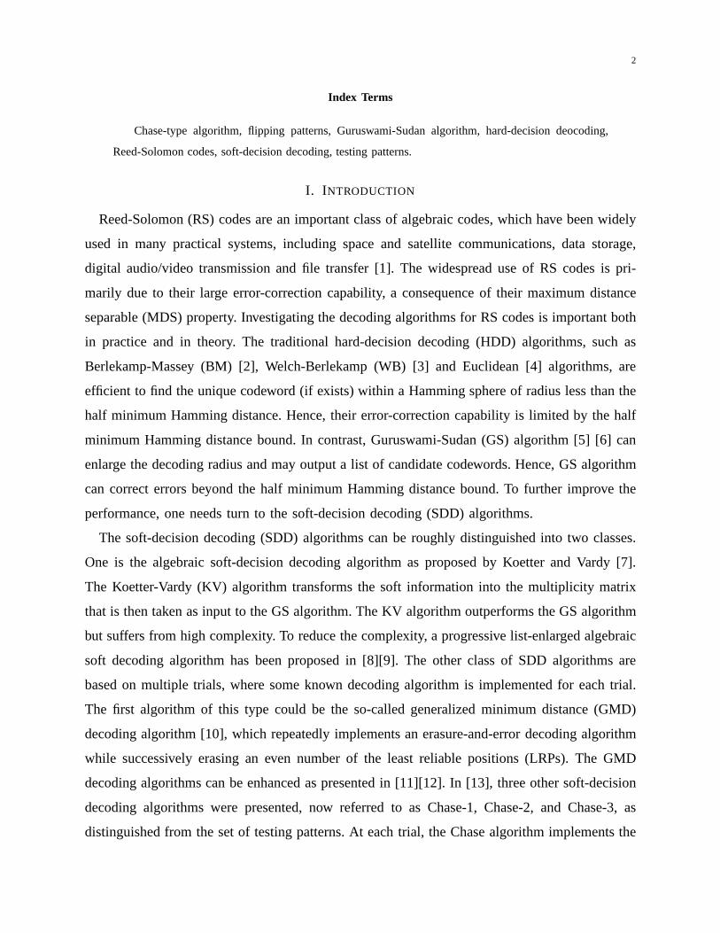
Fig. 3. Complexity of the tree-based Chase-type decoding ofthe RS codeC16[15, 11].

required for the TCGS algorithm are even less than those for the GMD algorithm whenSNR ≥

5.0 dB. �









19

4 4.5 5 5.5 6 6.5 710

−7

10−6

10−5

10−4

10−3

10−2

10−1

100

Eb/N

0(dB)

FE

R

GMDKVLCC( η = 3)TCGS( L = 8)LCC( η = 4)TCGS( L = 16)LCC( η = 6)TCGS( L = 64)LCC( η = 8)TCGS( L = 256)




5.25 dB. �








20

4 4.5 5 5.5 6 6.5 710

0

101

102

103

Eb/N

0(dB)

Itera

tions

GMDLCC( η = 8)TCGS( L = 256)LCC( η = 6)TCGS( L = 64)LCC( η = 4)TCGS( L = 16)LCC( η = 2)TCGS( L = 4)





5.75 dB. �

In summary, we have compared by simulation the tree-based Chase-type GS (TCGS) decoding

algorithm with the LCC decoding algorithm, showing that theTCGS algorithm has a better

performance and requires less trials for a given maximum testing number. We will not argue that

the proposed algorithm has lower complexity since it is difficult to make such a comparison. The

difficulty lies in that, although the interpolation processin the finite field is simple, the proposed

algorithm requires pre-processing and evaluating the lower bound for each flipping pattern in

21

4 4.5 5 5.5 6 6.5 710

−6

10−5

10−4

10−3

10−2

10−1

100

Eb/N

0(dB)

FE

R

GMDKVLCC( η = 4)TCGS( L = 16)LCC( η = 7)TCGS( L = 128)LCC( η = 9)TCGS( L = 512)


the real field. However, the proposed algorithm have the figure of merits as discussed in the

following subsections.

B. Decoding with A Threshold

Most existed Chase-type algorithms set a combinatorial number as the maximum testing

number, since they search the transmitted codeword within some Hamming sphere. In contrast,

the proposed algorithm can take any positive integer as the maximum testing number. Even

better, we can set a threshold of the soft weight to terminatethe algorithm. That is, the proposed

algorithm can be modified to exit wheneverB(f) ≥ Tz, whereTz is a tailored threshold related

to z. In the setting of BPSK signalling over AWGN channels, decoding with a threshold is

equivalent to searching the most-likely codeword within anEuclidean sphere, as outlined below.

22

4 4.5 5 5.5 6 6.5 710

0

101

102

103

Eb/N

0(dB)

Itera

tions

GMDLCC( η = 9)TCGS( L = 512)LCC( η = 7)TCGS( L = 128)LCC( η = 4)TCGS( L = 16)


Recall thatc, r andz are the transmitted codeword, the received vector and the hard-decision

vector, respectively. To trade off between the performanceand the complexity, we may search the

most-likely codeword within an Euclidean sphereS(r, T ) ∆= {s = φ(v) : ||r− s||2 < T}, where

φ(v) is the image ofv under the BPSK mapping. Equivalently, we may search all hypothesized

error patternse such that

λ(e) = log Pr{r|z} − log Pr{r|z− e} = (||r− φ(z− e)||2 − ||r− φ(z)||2)/(2σ2) < Tz,

whereTz = (T − ||r − φ(z)||2)/(2σ2) and σ2 is the variance of the noise. Hence, if we take

B(f) ≥ Tz as the final condition to terminate the tree-based Chase-type algorithm, we actually

make an attempt to avoid generating candidate codewords outside the sphereS(r, T ). This is

23

different from the decoding with a threshold mentioned in [13], where the lightest hypothesized

error pattern among all candidates is accepted only if its soft weight is less than a preset threshold.

Now the issue is how to choose the thresholdTz, or equivalently,T . On one hand, to guarantee

the performance, the sphereS(r, T ) is required to be large enough to contain the transmitted

codeword with high probability. On the other hand, a largeT usually incurs higher complexity.

Let ǫ > 0 be the error performance required by the user, meaning that the user is satisfied with

FER≈ ǫ. Then the user can find a thresholdT such thatPr{||r − φ(c)||2 ≥ T} = ǫ/2. This

can be done since||r − φ(c)||2/σ2 is distributed according to theχ2 distribution with n log q

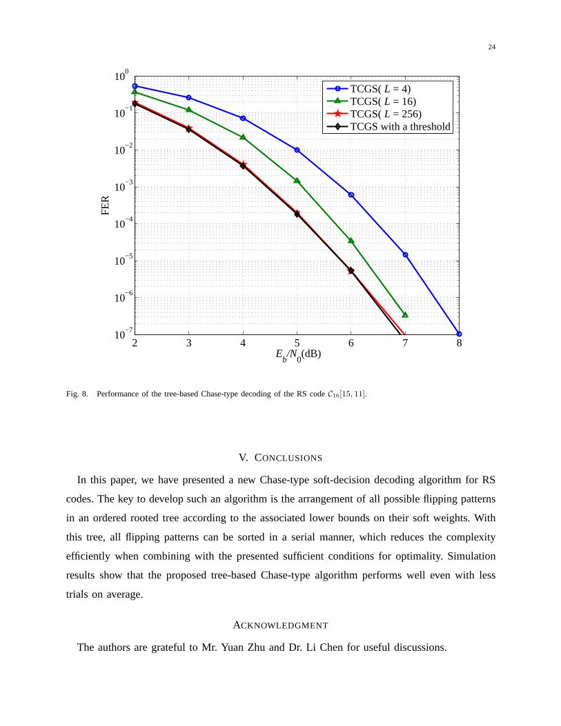
degrees of freedom. The simulation results forC16[15, 11] and C32[31, 25] are shown in Fig. 8

and Fig. 9, respectively. It can be seen that, forC16[15, 11], decoding with a threshold performs

almost the same as with a maximum number of trialsL = 256, while for C32[31, 25], decoding

with a threshold performs about0.7 dB better than with a maximum number of trialsL = 256.

C. Simulation-based Bounds on the ML Decoding

The proposed algorithm also presents a method to simulate the bounds on the maximum

likelihood decoding. LetE be a random variable such thatE = 1 if the ML decoding makes

an error andE = 0 otherwise. Since no ML decoding algorithm is available, we cannot use

simulation to evaluate the the probabilityPr{E = 1}. However, we can simulate bounds on the

ML decoding. Letc and c be the transmitted codeword and the estimated codeword fromthe

tree-based Chase-type decoder, respectively. We say thatc is verifiableif it satisfies the sufficient

conditions presented in Theorem 3 or Theorem 4.

There are four cases.

• Case 1. Ifc = c and c is verifiable,Eu = Eℓ = E = 0;

• Case 2. Ifc = c but c is not verifiable, defineEu = 1 andEℓ = 0;

• Case 3. Ifc 6= c and c is more likely thanc, Eu = Eℓ = E = 1;

• Case 4. Ifc 6= c and c is less likely thanc, Eu = 1 andEℓ = 0.

Obviously,Eℓ ≤ E ≤ Eu. SinceEℓ andEu can be simulated, we can get simulation-based

bounds on the ML decoding. The simulation-based bounds on the ML decoding of the RS code

C16[15, 11] are shown in Fig 10. It can be seen that the upper bound and the lower bound are

getting closer as the number of trials increases, implying that the proposed algorithm is near

optimal withL ≥ 256 at SNR= 5.0 dB.

24

2 3 4 5 6 7 810

−7

10−6

10−5

10−4

10−3

10−2

10−1

100

Eb/N

0(dB)

FE

R

TCGS( L = 4)TCGS( L = 16)TCGS( L = 256)TCGS with a threshold


V. CONCLUSIONS

In this paper, we have presented a new Chase-type soft-decision decoding algorithm for RS

codes. The key to develop such an algorithm is the arrangement of all possible flipping patterns

in an ordered rooted tree according to the associated lower bounds on their soft weights. With

this tree, all flipping patterns can be sorted in a serial manner, which reduces the complexity

efficiently when combining with the presented sufficient conditions for optimality. Simulation

results show that the proposed tree-based Chase-type algorithm performs well even with less

trials on average.

ACKNOWLEDGMENT

The authors are grateful to Mr. Yuan Zhu and Dr. Li Chen for useful discussions.

25

4 4.5 5 5.5 6 6.5 710

−7

10−6

10−5

10−4

10−3

10−2

10−1

100

Eb/N

0(dB)

FE

R

TCGS( L = 8)TCGS( L = 16)TCGS( L = 64)TCGS( L = 256)TCGS with a threshold


APPENDIX A

THE M INIMALITY OF THE M INIMAL DECOMPOSITION

There are exactlyqk hypothesized error patterns, which collectively form a coset of the code,

E = {e = z−c : c ∈ C}. For everyf ∈ Fnq , when takingz− f as an input vector, the conventional

HDD either reports a decoding failure or outputs a unique codewordc. In the latter case, we say

that the flipping patternf generatesthe hypothesized error patterne = z− c. It can be verified

that there exist∑

0≤t≤tmin

(nt

)qt flipping patterns that can generate the same hypothesized error

pattern. In fact, for eache ∈ E , defineF(e) = {f : e = f + g,WH(g) ≤ tmin}, which consists of

all flipping patterns that generatee.

Proposition 5: Let e be a hypothesized error pattern andf be its associated minimal flipping

26

2 4 6 8 10 1210

−5

10−4

10−3

10−2

10−1

log2( L)

FE

R

ML upper boundML lower boundTCGS

Fig. 10. Simulation-based bounds on the ML decoding of the RScodeC16[15, 11] at 5.0 dB.

pattern. Thenf ∈ F(e), λ(f) = minh∈F(e) λ(h) andRu(f) = minh∈F(e)Ru(h).

Proof: Sincee is a hypothesized error pattern,c = z−e is a codeword, which can definitely

be found whenever the HDD takes as input a vectorc + g with WH(g) ≤ tmin. That is,e can

be generated by takingz − h (with h = e − g) as the input to the HDD. Letf ∈ F(e) be a

flipping pattern such thatλ(f) = minh∈F(e) λ(h). It suffices to prove that, forWH(e) > tmin and

e = f + g, we haveg ∈ G(f), i. e., |S(g)| = tmin, S(f)⋂S(g) = ∅ andRu(f) < Rℓ(g). This can

be proved by contradiction.

Suppose that|S(g)| < tmin. Let (i1, γ1) be a nonzero component off. Then e can also be

generated byf− (i1, γ1), whose soft weight is less than that off, a contradiction to the definition

of f.

27

Suppose thatS(f)⋂S(g) 6= ∅. Let i1 ∈ S(f)

⋂S(g) and (i1, γ1) be the nonzero component

of f. Then e can also be generated byf − (i1, γ1), whose soft weight is less than that off, a

contradiction to the definition off.

Obviously,Ru(f) 6= Rℓ(g) since their support sets have no common coordinates. Suppose that

Ru(f) > Rℓ(g). Let (i1, γ1) be the atom with rankRu(f) and (i2, γ2) be the atom with rank

Rℓ(g). Thene can also be generated byf− (i1, γ1)+ (i2, γ2), whose soft weight is less than that

of f, a contradiction to the definition off.

REFERENCES

[1] D. J. Costello Jr., J. Hagenauer, H. Imai, and S. B. Wicker, “Applications of error-control coding,”IEEE Trans. Inform. The-

ory, vol. 44, no. 6, pp. 2531–2560, 1998.

[2] E. R. Berlekamp, “Nonbinary BCH decoding,”IEEE Trans. Inform. Theory, vol. IT-14, p. 242, 1968.

[3] L. Welch and E. R. Berlekamp, “Error correction for algebraic block codes,” inProc. IEEE Int. Symp. Inform. Theory, St.

Jovites, Canada, 1983.

[4] M. Sugiyama, M. Kasahara, S. Hirawawa, and T. Namekawa, “A method for solving key equation for decoding Goppa

codes,”Inform. Contr., vol. 27, pp. 87–99, 1975.

[5] M. Sudan, “Decoding of Reed Solomon codes beyond the error-correction bound,”Journal of Complexity, vol. 13, no. 1,

pp. 180–193, 1997.

[6] V. Guruswami and M. Sudan, “Improved decoding of Reed-Solomon and algebraic-geometric codes,”IEEE Trans. In-

form. Theory, vol. 45, no. 6, pp. 1757–1767, Sep. 1999.

[7] R. Koetter and A. Vardy, “Algebraic soft-decision decoding of Reed Solomon codes,”IEEE Trans. Inform. Theory, vol. 49,

pp. 2809–2825, 2003.

[8] S. Tang, L. Chen, and X. Ma, “Progressive list-enlarged algebraic soft decoding of Reed-Solomon codes,”IEEE Commu-

nications Letters, vol. 16, no. 6, pp. 901–904, 2012.

[9] L. Chen, S. Tang, and X. Ma, “Progressive algebraic soft-decision decoding of Reed-Solomon codes,”IEEE Trans. Com-

mun., vol. 61, no. 2, pp. 433–442, 2013.

[10] G. D. Forney Jr., “Generalized minimum distance decoding,” IEEE Trans. Inform. Theory, vol. IT-12, no. 2, pp. 125–131,

Apr. 1966.

[11] R. Kotter, “Fast generalized minimum-distance decoding of algebraic-geometry and Reed-Solomon codes,”IEEE Trans. In-

form. Theory, vol. 42, pp. 721–737, May 1996.

[12] S.-W. Lee and B. V. Kumar, “Soft-decision decoding of reed-solomon codes using successive error-and-erasure decoding,”

in Proc. IEEE Global Telecommun. Conf., New orleans, LA, Nov. 2008, DOI: 10.1109/GLOCOM.2008.ECP.588.

[13] D. Chase, “A class of algorithms for decoding block codes with channel measurement information,”IEEE Trans. In-

form. Theory, vol. IT-18, pp. 170–182, Jan. 1972.

[14] H. Tang, Y. Liu, M. Fossorier, and S. Lin, “On combining Chase-2 and GMD decoding algorithms for nonbinary block

codes,”IEEE Communications Letters, vol. CL-5, pp. 209–211, 2001.

[15] X. Zhang, Y. Zheng, and Y. Wu, “A Chase-type Koetter-Vardy algorithm for soft-decision Reed-Solomon decoding,” in

Computing, Networking and Communications (ICNC), 2012 International Conference on, pp. 466–470.

28

[16] M. P. Fossorier and S. Lin, “Soft-decision decoding of linear block codes based on ordered statistics,”IEEE Trans. In-

form. Theory, vol. 41, no. 5, pp. 1379–1396, 1995.

[17] J. Jiang and K. R. Narayanan, “Iterative soft-input soft-output decoding of Reed-Solomon codes by adapting the parity-

check matrix,”IEEE Trans. Inform. Theory, vol. 52, no. 8, pp. 3746–3756, 2006.

[18] J. Bellorado, A. Kavcic, M. Marrow, and L. Ping, “Low-complexity soft-decoding algorithms for Reed-Solomon codes—

Part II: Soft-input soft-output iterative decoding,”IEEE Trans. Inform. Theory, vol. 56, no. 3, pp. 960–967, Mar. 2010.

[19] J. Bellorado and A. Kavcic, “Low-complexity soft-decoding algorithms for Reed-Solomon codes—Part I: An algebraic

soft-in hard-out Chase decoder,”IEEE Trans. Inform. Theory, vol. 56, no. 3, pp. 945–959, Mar. 2010.

[20] J. Zhu, X. Zhang, and Z. Wang, “Backward interpolation architecture for algebraic soft-decision Reed-Solomon decoding,”

Very Large Scale Integration (VLSI) Systems, IEEE Transactions on, vol. 17, no. 11, pp. 1602–1615, 2009.

[21] T. Kaneko, T. Nishijima, H. Inazumi, and S. Hirasawa, “An efficient maximum-likelihood-decoding algorithm for linear

block codes with algebraic decoder,”IEEE Trans. Inform. Theory, vol. 40, no. 2, pp. 320–327, Mar. 1994.

[22] V. Guruswami and A. Vardy, “Maximum-likelihood decoding of Reed-Solomon codes is NP-hard,”IEEE Trans. In-

form. Theory, vol. 51, no. 7, pp. 2249–2256, 2005.

[23] X. Ma and S. Tang, “Correction to ‘an efficient maximum-likelihood-decoding algorithm for linear block codes with

algebraic decoder’,”IEEE Trans. Inform. Theory, vol. 58, no. 6, p. 4073, 2012.

[24] R. J. McEliece, “The Guruswmi-Sudan decoding algorithm for Reed-Solomon codes,” IPN Progress Rep., Tech. Rep.

42-153, 2003.

Documents

1 A New Chase-type Soft-decision Decoding Algorithm for