2008

WindSim Validation Study CFD validation in Complex terrain Tristan Wallbank

2 | P a g e

1 Executive Summary The following report documents a study carried out to validate the WindSim software in its application to the wind turbine industry. WindSim is a user interface for the CFD application software Phoenics and is based on solving the Reynolds Averaged Navier-Stokes flow equations. This validation is achieved by comparing the model outputs to known values obtained from field measurements using standard meteorology equipment and arrangements. Additional to the validation of this software, a comparison of the WindSim CFD software is made with industry standard linear flow models, namely WAsP and WAsP Engineering in order to gauge the apparent benefits of employing CFD flow models to estimate climatic parameters. The climatic parameters investigated in this study were horizontal wind speed, wind frequencies, turbulence intensity and inflow angles. Additional to these parameters, the models were tested on how well they estimated different heights (height extrapolation). Two sites were used in this study with both sites being broken down into two separate sub-sites. The first because of issues relating to overlapping data, and the second due to the sheer size of the parent site. The approach to this study was to employ a two part testing regime. The first of these was dubbed the “Sensitivity Analysis” and involved the testing of the various user definable parameters in WindSim using part of the data set of a single site to yield results for mean wind speeds and turbulence intensities. This was done to gain a greater understanding on how these parameters changed the prediction of the climatic parameters and also to obtain an optimal mix of parameters to adopt in the full test runs. The second part of the testing was the full test runs. The results of these test runs for all four sub sites were compared with the equivalent results of the linear flow models. WAsP was employed for predicting mean wind speeds (with delta RIX corrections applied) and wind frequencies, and WAsP Engineering for predicting inflow angles and turbulence intensity (with a correction factor applied to both the WAsP Engineering and WindSim turbulence intensity results recommended by both software developers). The results from the Sensitivity Analysis showed a relatively low sensitivity of the mean wind speed predictions to the majority of the tested parameters apart from the forestry feature with high errors from this parameter. The Forest feature also tended to create large prediction errors for the turbulence intensity. Unfortunately, when comparing the equivalent mast and sector results from the full test runs with those of the baseline case of the Sensitivity Analysis, the expected increase in accuracy of applying the findings of the Sensitivity Analysis did not occur.

3 | P a g e

The full test results yielded interesting results. Overall the two model types (WAsP and WindSim) behaved in a similar fashion for all climatic parameter predictions. This was both in magnitude of the error and the tendency to over or under predict. With respect to the calculation of mean wind speed, there was little overall difference between WindSim and WAsP, with WindSim slightly the better performing of the two models. WindSim did calculate the per-sector mean wind speed and frequencies better than WAsP which does indicate an advantage to the CFD model in capturing the finer detail of the flow. For the sub sites in this study the application of delta RIX corrections to the WAsP wind speed prediction results was seen to have overall poor results. Apart from the case of a single sub-site, the corrections generally increased the inaccuracies of the WAsP results. In terms of height extrapolation of the two models, it was seen that a general under prediction for predictions to higher levels, and a general over prediction for predictions to lower levels resulted. This highlights the requirement for care required when using models to extrapolate to different levels and the requirement for close to hub height level monitoring to reduce uncertainties in wind resource calculations. The results of the turbulence intensity values had a tendency to over predict, with or without the corrections. This showed that the model output corrections recommended by both software developers (effectively scaling the turbulence intensity result by 4/3) may not be the best approach for dealing with the outputs from the WindSim and WAsP Engineering models. A simple method of scaling the turbulence intensity values based on the errors from the prediction of known measurements employed in this study was seen to help the accuracy of turbulence intensity predictions. The inflow angle predictions of the WindSim and WAsP Engineering models proved to be largely similar with the highest errors of the two quality-controlled data sets being around 3 degrees. It is recommended that future inflow angle tests are performed for more extreme cases, using validation data sets of known high inflow angles in excess of +/- 8 degrees. In terms of project shortcomings, it was an undesired result of hardware inadequacies that the final model resolutions were relatively coarse. With a maximum model resolution of between 35m and 45m for the four sites, it is believed that the true power of CFD modelling was not realised and future studies should be based on using much higher hardware specifications, particularly in relation to the available RAM. 16GB to 32GB is recommended for this (in comparison to the 4GB of RAM used for this study). Preferable grid size resolution of 10m or less is recommended.

4 | P a g e

Over all, the two model types showed to have their respective advantages and disadvantages. The major advantage of the linear models, WAsP and WAsP Engineering, came primarily from their simplicity. This simplicity derives from both their ease of use (the recommended requirements for a WAsP or WAsP Engineering user is not as demanding as that of a CFD user), speed of calculations and manageable output sizes. In comparison, the WindSim modelling for this study took over 550 hours of modelling (over three months based on a 40 hr week) and generated close to 100GB of output data. Additionally, without extremely high specification hardware, the desired resolution cannot be achieved. The advantages of the WindSim model over its linear model counterparts appear to be in the detail that the results capture on a per sector basis. Additional to this, but not studied over the course of the current study, is the strong visual interface that WindSim offers. And with a particle tracing feature, areas of modelled recirculation can be identified, a feature which can aid the wind farm designer to avoid high risk areas.  A great deal was learnt in this study on WindSim and CFD modelling in general. This includes but is not limited to knowledge on different solver types, different CFD calculation types (e.g. RANS vs LES), realistic hardware requirements and the importance of different stability cases.  

5 | P a g e

Contents 1  Executive Summary .................................................................................. 2 2  Introduction ............................................................................................. 7 3  Background ............................................................................................. 8 

3.1  Governing equations........................................................................... 8 3.1.1  Navier-Stokes equations ............................................................... 8 3.1.2  Navier-Stokes Equations and Turbulence ......................................... 8 3.1.3  Reynolds Averaged Navier-Stokes Equations .................................... 9 3.1.4  WindSim Reynolds Averaged Navier-Stokes equations ....................... 9 

3.2  Other CFD techniques ........................................................................ 10 3.2.1  Direct Numerical Simulation (DNS) ................................................ 10 3.2.2  Large eddy simulation (LES) ......................................................... 10 3.2.3  Detached eddy simulation (DES) ................................................... 10 

3.3  Turbulence ....................................................................................... 11 3.3.1  Reynolds number and Turbulence .................................................. 12 3.3.2  Richardson’s energy cascade ........................................................ 12 3.3.3  Turbulent Kinetic Energy .............................................................. 13 3.3.4  TKE Budget ................................................................................ 13 3.3.5  k-epsilon turbulence model........................................................... 14 3.3.6  TKE vs TI ................................................................................... 15 

3.4  WindSim features .............................................................................. 16 3.4.1  Terrain ...................................................................................... 16 3.4.2  Wind Fields ................................................................................ 17 3.4.3  Objects ...................................................................................... 17 3.4.4  Results ...................................................................................... 17 3.4.5  Wind Resource ........................................................................... 17 3.4.6  Energy ...................................................................................... 18 

3.5  WAsP .............................................................................................. 18 3.5.1  DELTA-RIX ................................................................................. 21 

3.6  WAsP Engineering ............................................................................. 22 4  Project Aim ............................................................................................. 24 5  Methodology ........................................................................................... 24 

5.1  Data ............................................................................................... 24 5.2  Validation ........................................................................................ 25 5.3  Hardware ......................................................................................... 25 5.4  Software .......................................................................................... 26 

6  Test Sites ............................................................................................... 26 6.1  Site A .............................................................................................. 26 6.2  Site B .............................................................................................. 26 6.3  Data Sets ........................................................................................ 27 

6.3.1  Site A ........................................................................................ 27 6.3.2  Site B ........................................................................................ 28 

7  WindSim Sensitivity Analysis ..................................................................... 30 7.1  Test Parameters ............................................................................... 30 

7.1.1  Test 1: Baseline Test Parameters .................................................. 30 7.1.2  Test 2: Coupled vs Segregated solver ............................................ 34 7.1.3  Test 3: Turbulence Model – Standard k-epsilon vs Modified ............... 34 7.1.4  Test 4: Forest vs No Forest .......................................................... 35 7.1.5  Test 5: Terrain Smoothing vs No Terrain Smoothing ........................ 37 7.1.6  Test 6: Number of cells in Z Direction. ........................................... 39 

7.2  Results ............................................................................................ 39 7.2.1  Wind speeds ............................................................................... 39 

6 | P a g e

7.2.2  Turbulence ................................................................................. 42 7.3  Conclusions from Sensitivity Analysis ................................................... 45 

8  Full Test results ....................................................................................... 46 8.1.1  Delta RIX settings ....................................................................... 47 8.1.2  Model Grid Spacing ..................................................................... 47 

8.2  Wind Speed Prediction ....................................................................... 48 8.3  Delta Rix Corrections ......................................................................... 52 8.4  Prediction of different heights ............................................................. 53 8.5  Turbulence Intensity Prediction ........................................................... 56 8.6  Inflow Angle Prediction ...................................................................... 59 

9  Recommendations/Future Research ............................................................ 62 10  Conclusions ......................................................................................... 64 11  References .......................................................................................... 66 12  Appendix ............................................................................................ 68 

12.1  Sensitivity Analysis: .......................................................................... 68 12.1.1  Wind Speed................................................................................ 68 12.1.2  Turbulence Intensity .................................................................... 72 

12.2  Full Tests ......................................................................................... 75 12.2.1  Wind Speed................................................................................ 75 12.2.2  TI ............................................................................................. 83 

12.3  Navier-Stokes Equations .................................................................... 87 12.3.1  Conservation of Momentum .......................................................... 87 12.3.2  Conservation of Mass ................................................................... 88 12.3.3  Incompressible Flow .................................................................... 88 

7 | P a g e

2 Introduction WindSim is a user interface for the CFD application software called Phoenics developed by Cham (UK). WindSim is designed for wind flow and resource calculations specifically for wind energy projects. It is based on a mesh system of modelling the wind and terrain in the model. This uses a Phoenics based 3-dimensional Reynolds Averaged Navier-Stokes solver to resolve the wind conditions in each of the cells in the mesh system. Due to the increasing trend of developing wind farms in complex terrain particularly in New Zealand, there is a need for reliable and practical software for this sort of terrain. The current industry standard software tools (WAsP and WAsP Engineering) were not designed with complex terrain sites in mind and as they use a linear flow model, they do not account for the flow separation that high complexity sites and varying roughness situations induce. WAsP was initially developed twenty years ago for typical Danish sites and the flow model has not changed a great deal since. Calculations of climatic parameters for the majority of wind farm sites have historically relied on laminar flow models. There have been various cases around the world where wind turbines have undergone either structural or mechanical failure largely due to insufficient knowledge of the site conditions. Accurate knowledge of the wind resource at a site and the accurate transferral of the measured wind conditions to potential wind turbine positions are also essential, relating directly to the economic predictions of the output of the site. Due to the large investments made in these projects, a greater understanding of site climatic parameters is desired by turbine manufacturers and project owners alike. CFD modelling is generally regarded as having the ability to deliver greater certainty. Due to high computational demands and the detailed knowledge required for the use of most CFD codes due to their complexity, the industry standard software WAsP is still generally used in analysing complex sites. However this entails acceptance of a greater degree of uncertainty in the project outcome. WindSim is attractive because it provides a user friendly interface (comparable to the WAsP interface). Although it still requires significant computational power to run model sizes of any practical relevance to commercial scale wind farms, it is a wind industry dedicated CFD interface. Hence the inputs and outputs are compatible with other wind industry standard software packages such as WindPro and WAsP, which greatly enhances its usability. A warning, however, should be extended to anyone considering an “off the shelf” CFD package such as WindSim. The proficient and competent use of CFD software requires a great deal of experience in a variety of backgrounds. Reliable outputs from CFD software preferably should come from a user with at least 3-5 years of experience working in this field with a thorough background in Fluid Dynamics, Turbulence Modelling, Mechanical Engineering and IT. Throughout this project the reader should bear in mind that it has been performed by a comparative CFD novice regardless of the “of the shelf” environment that WindSim brings. This study proposes to test the accuracy and viability of WindSim as a wind farm calculation tool, reviewing not only energy calculation but also wind load parameters such as turbulence and inflow angle.

8 | P a g e

It is the intention that Suzlon and wind farm developers involved in this study will learn a great deal as to the practicality of WindSim as a tool for use in the analysis of complex terrain sites and gain further knowledge into CFD modelling in general. As such, this report is written with both an academic audience and an industry audience in mind.

3 Background

3.1 Governing equations The WindSim model is based on Reynolds Averaged Navier-Stokes equations for an incompressible flow. A brief introduction to these equations is provided below.

3.1.1 Navier­Stokes equations  The Navier-Stokes equations, named after Claude-Louis Navier and George Gabriel Stokes, are an application of Newton’s second law (F=ma) and describe the motion of fluids such as liquids and gases. These equations have wide ranging applications, from modelling weather and ocean currents to the flow around an airfoil. The Navier-Stokes equations are non-linear, partial differential equations. These do not establish an explicit relationship between the variables of interest, rather they establish associations of rates of change which link the variables. A solution of the Navier-Stokes equations is called a velocity field and describes the velocity of the fluid at a point in time (they do not explicitly describe the position of a fluid particle). The Navier-Stokes equations appear to model the motion of most fluids well, however the complicated nature of the equations usually limits their widespread use to Newtonian fluids (for which time tested formulations exist). For non-Newtonian fluids, complicated formulations result which render the equations extremely difficult to deal with. This stems from a higher number of unknown variables compared to the equations to be solved The Navier-Stokes equations are based on the assumption that the fluid is a continuous substance (and not a discrete collection of particles). The derivation of the Navier-Stokes equations begins with the conservation of mass, momentum and (optionally) energy being written for a control volume (a finite arbitrary volume). Refer to the Appendix section 12.3 for further detail.

3.1.2 Navier­Stokes Equations and Turbulence  It is believed that the Navier-Stokes equations model turbulence properly (1). However the numerical solution of the Navier-Stokes equations for turbulent flow presents many difficulties, mainly in the form of the extremely fine mesh required to capture the full range of length scales and the unfeasibly large computational power and time involved. As such, turbulence is often handled in a “statistical” as opposed to an explicit way, and methods such as the k-e model (refer to section 3.3.5) are employed in practical CFD applications to model turbulent flow. This approach also

9 | P a g e

accounts for the unknowns in the governing equations when dealing with turbulent flow and is referred to as “Turbulence Closure” (2). Refer to section 3.3.

3.1.3 Reynolds Averaged Navier­Stokes Equations  The key thing to note about Reynolds Averaged Navier-Stokes (RANS) equations are that these are “time averaged” Navier-Stokes equations and as referred to above, these are primarily used when modelling turbulent flow. The name of the equation comes from the fact that the “Reynolds decomposition” is applied to the Navier-Stokes equations. The Reynolds decomposition defines that a flow variable may be separated into the mean component (a time averaged component) and the fluctuating component.

, ,   Equation 1 

Where X = (x,y,z) is the positional vector, the time averaged component and , the fluctuating component.

3.1.4 WindSim Reynolds Averaged Navier­Stokes equations  WindSim, via the Phoenics calculation engine, employs Reynolds Averaged Navier-Stokes equations to model the flow field. As opposed to a time step approach to solving flow calculations, this solution starts from the initial boundary conditions specified by the user and arrives at a steady state solution (which reflects a time averaged solution). This solution has one wind and one turbulence distribution for the entire domain (3). The Navier-Stokes equations as described by the WindSim software developer (4) are given in Cartesian tensor form as:

0

Equation 2

Here U is the velocity, x is the positional component, P is the pressure, ρ is the density, v is the kinematic viscosity and the subscripts i and j defining unit vectors. With turbulence closure obtained by relating the Reynolds stresses to the mean velocity through turbulent viscosity.

Equation 3

Where vT is the turbulent viscosity and k is the turbulent kinetic energy. For further information please refer to Arne Gravdahl’s paper (4).

10 | P a g e

3.2 Other CFD techniques Other common CFD techniques exist which differ from the RANS approach which WindSim is based on. These are introduced below.

3.2.1 Direct Numerical Simulation (DNS)  This is a simulation in which the complete set of Navier-Stokes equations are numerically solved in their entirety (so no turbulence model or Reynolds averaging is incorporated). This means that the full range of spatial and temporal scales of turbulence must be resolved (down to the “Kolmogorov” or microscales). There are mesh requirements which can be calculated depending on the spatial scale of boundary conditions as well as the size of the Reynolds number and the time step necessary also becomes a function of the Reynolds number. Generally speaking the computer power required to resolve these models with current computing capabilities makes DNS highly impractical for CFD applications, however DNS is useful in the development of turbulence models or for smaller numerical experiments which provide information unattainable from laboratory tests.

3.2.2 Large eddy simulation (LES)  In 1941, the Russian mathematician Andrey Kolmogorov postulated that large eddies are dependent on flow geometry while smaller eddies have a universal character (for very high Reynolds numbers the statistics of small scale eddies depend only on the viscosity and the rate of energy dissipation) (5). Although the energy dissipation rate varies in space and time, the Kolmogorov theory uses the mean dissipation rate to represent typical small scales. Large eddy simulation (LES) solves the filtered Navier-Stokes equations explicitly for large scale eddies while using a turbulence model for smaller or so called “sub-grid” scales. The sub-grid models compensate for the unresolved turbulence via the addition of an “eddy viscosity” term into the Navier-Stokes equations. This sub grid “cut-off” point is often on the scale of 100m (2). LES requires less computational power than DES techniques but more than RANS techniques. The additional computer requirements manifests itself with improved levels of detail and increased accuracy over RANS methods, particularly for flows involving flow separation. While RANS methods provide a time averaged result, LES methods are able to resolve turbulent flow structures and predict instantaneous flow characteristics.

3.2.3 Detached eddy simulation (DES)  LES has issues when trying to model near walls and the computational demands increase significantly in these areas for the model to resolve completely. To counter this, a zonal approach can be adopted which runs RANS near walls and situations where the turbulent length scale is too small to be explicitly solved via LES. This compromise approach, which in effect is a hybrid RANS-LES model, is known as a

11 | P a g e

detached eddy simulation (DES) and provides a single smooth velocity field between the RANS and LES regions of the model.

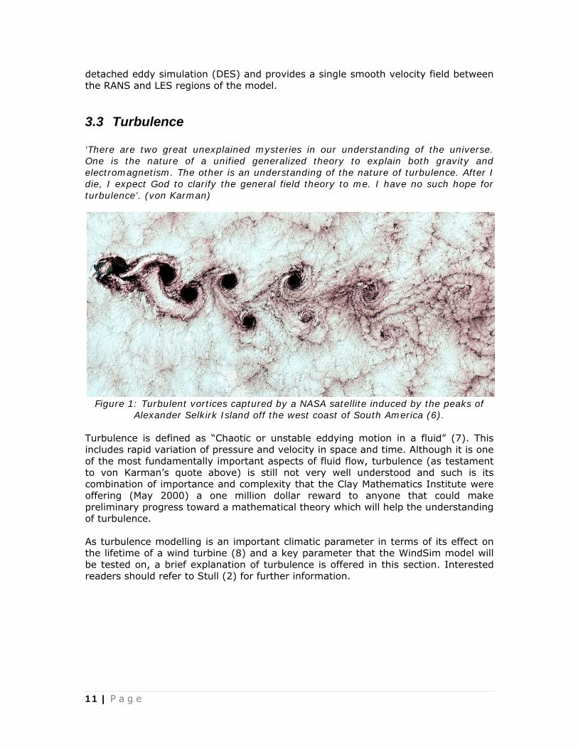
3.3 Turbulence ‘There are two great unexplained mysteries in our understanding of the universe. One is the nature of a unified generalized theory to explain both gravity and electromagnetism. The other is an understanding of the nature of turbulence. After I die, I expect God to clarify the general field theory to me. I have no such hope for turbulence’. (von Karman)

Figure 1: Turbulent vortices captured by a NASA satellite induced by the peaks of

Alexander Selkirk Island off the west coast of South America (6). Turbulence is defined as “Chaotic or unstable eddying motion in a fluid” (7). This includes rapid variation of pressure and velocity in space and time. Although it is one of the most fundamentally important aspects of fluid flow, turbulence (as testament to von Karman’s quote above) is still not very well understood and such is its combination of importance and complexity that the Clay Mathematics Institute were offering (May 2000) a one million dollar reward to anyone that could make preliminary progress toward a mathematical theory which will help the understanding of turbulence. As turbulence modelling is an important climatic parameter in terms of its effect on the lifetime of a wind turbine (8) and a key parameter that the WindSim model will be tested on, a brief explanation of turbulence is offered in this section. Interested readers should refer to Stull (2) for further information.  

12 | P a g e

3.3.1 Reynolds number and Turbulence  High Reynolds numbers define turbulent flow, and as such, turbulence is affected by the viscosity of a fluid, the density of a fluid or the length scale.

Equation 4

Where Re is the Reynolds number, d is the characteristic length scale, U is the wind velocity and v is the kinematic viscosity (viscosity normalised by density). Turbulence plays an important part in transporting heat, energy and mass in the atmosphere (9). Shear forces cause what is defined as mechanical turbulence while buoyant instabilities cause convective turbulences. Both forms of turbulence exist in atmospheric conditions. Refer to section 3.3.4.

3.3.2 Richardson’s energy cascade  Lewis Richardson’s turbulence theory stated that turbulent flow is made up of different sizes or “scales” of eddies. The large scales are unstable and eventually break up into smaller eddies. The kinetic energy of the original larger eddies is correspondingly divided into the smaller child eddies. These smaller eddies, in turn, break up and spawn smaller eddies again. Thus there is an energy cascade with energy being passed along the scale of eddies. Eventually the eddies will get to a critical size where viscous forces will dissipate the energy internally (into heat). This final scale is known as the “Kolmogorov microscale”, and typical scales are in the range of 10-3m. As a comparison, the largest scale eddies can have lengths on the order of up to three kilometres (the scale of the depth of the planetary boundary layer). Figure 2: Illustration of Richardson’s Energy Cascade – the degradation of turbulent

eddies.

Heat Dissipation

13 | P a g e

3.3.3 Turbulent Kinetic Energy   WindSim uses the calculation of turbulent kinetic energy to derive TI results (refer to section 3.3.6 below). The following is a brief explanation on what turbulent kinetic energy is. Interested readers should refer to Stull (2) for further information. Kinetic Energy (KE) can be thought of as being able to be broken down into two portions, one associated with the mean wind (Mean Kinetic Energy (MKE)), the other associated with the turbulent wind (Turbulent Kinetic Energy (TKE)). Kinetic energy is defined as:

0.5 Equation 5 Where m = mass and Ui = wind speed. Broken down into the two above mentioned sub components (TKE and MKE) for each direction (x, y and z), KE can be represented by the following two equations.

Equation 6

Equation 7

Where e represents an instantaneous TKE per unit mass. And by averaging e, a more direct TKE relationship is derived given as:

Equation 8

3.3.4 TKE Budget   Turbulent Kinetic Energy can be estimated via the TKE budget. The TKE budget allows for the production, storage, advection and dissipation of TKE. The budget is included here to illustrate to the reader the different processes involved in estimating TKE. Assuming the coordinate system is aligned with the mean wind, this is given below as:

– Equation 9

I II III IV V VI

14 | P a g e

Where: Term I = storage or tendency of TKE Term II = buoyant production or consumption term (related to heat flux) Term III = mechanical shear Term IV = TKE Transport term (not by advection but by turbulent eddies) Term V = pressure correlation term (how TKE is transported by pressure

perturbations) Term VI = viscous dissipation of TKE - conversion to heat Refer to Stull (2) for a full explanation of each of the above given parameters.  

3.3.5 k­epsilon turbulence model  The k-epsilon turbulence model is a two equation turbulence model, common in CFD application, which includes two additional transport equations to model turbulence. This is how WindSim calculates the turbulence. The first of these two equations describes the turbulent kinetic energy (which determines the energy in the turbulence) while the second equation describes the turbulent dissipation (which determines the scale of the turbulent structure). From Arne Gravdahl’s paper (4), and using the same notation as section 3.1.4, the k-epsilon model is given as:

Equation 10

Equation 11

Equation 12

Where Cμ, σk, σε, Cε1 and Cε2 are constants as defined in Table 1 and Table 2 below and Pk is the turbulent kinetic energy production term given as:

Equation 13

The k-epsilon model constants take on the values as given in Table 1 below.

Cμ  σk σε Cε1 Cε20.09 1.0 1.3 1.44 1.92 Table 1: Standard k-epsilon model constants

15 | P a g e

For the modified turbulence model applied in WindSim, the model uses the same k-epsilon model, however the constants as shown in Table 1 have been changed. The changes come from “tuning” these constants to better describe the turbulence as experienced in a neutral atmospheric boundary layer. The modified constants are provided in Table 2 (refer to section 7.1.3 for their application).

Cμ  σk σε Cε1 Cε20.0324 1.0 1.85 1.44 1.92 Table 2: Modified k-epsilon model constants

3.3.6 TKE vs TI  Turbulence Intensity (TI) as dealt with by the IEC61400 series of standards (pertaining to Wind turbines) is an industry wide norm for representing turbulence. Turbulence Intensity as measured by a cup anemometer is defined as:

/ Equation 14

Where σ is the standard deviation of the measured wind speed and uH is the mean horizontal component of wind velocity (which can be thought of as the RMS of the velocities in the x and y direction respectively) determined from the same wind data sample. TI can also be represented for a single direction (say x) as:

√

Equation 15 And for the horizontal TI (x and y combined) this is represented as:

√

Equation 16

Through this relationship, the TI can be derived from the TKE and velocity components, which, along with assuming isotropic turbulence, is how WindSim calculates the TI. WindSim is based on the assumption of a neutrally stable atmosphere. Under these assumptions, the TI is independent of wind speed. The assumption of a neutrally stable atmosphere is often a good approximation at higher wind speeds (~>15ms) however this is not always the case and care must be employed when dealing with models making these assumptions (3). The software developer has recommended comparing the model outputs to measured TI values at 15m/s after applying the same correction factor that RISØ recommends for its WAsP Engineering model outputs (10). Refer to sections 3.6, 7.2 and 8.5 for how this was handled in the current study.

16 | P a g e

3.4 WindSim features The WindSim software, a user interface for the CFD software PHOENICS, has 6 different hierarchal calculation modules, the first three of which will only run when the former has been correctly calculated, and the last three will only run if all of the first three have been calculated. These are briefly explained below. For more information on the software, refer to www.windsim.com and reference (11).

3.4.1 Terrain The first of these modules is where the terrain model is loaded, modified and checked. The software accepts terrain grid data in .GWS format (which can be a combined height contour and roughness map, converted from the WAsP .MAP format). Here options of defining the area of the map to be used, general grid set-up (node spacing etc) and employment of the forest model (refer forest section in SA) can be specified. Refinement of the meshed grid can also be specified here. Refinement is where the spacing of the nodal points are closely packed at the area of interest in the x and y horizontal directions and once outside the area of interest, these are increasingly spaced away from the refined area all the way to the boundary. This method allows a higher resolution of the area of interest while still allowing a manageable amount of cell numbers (refer to Figure 3 below). Refinement can only be selected in the final nested layer as this prevents the possibility of further nesting.

Figure 3: Illustration of WindSim cell refinement feature  

17 | P a g e

3.4.2 Wind Fields The second module calculates the wind fields (based on user defined boundary conditions) and solves, for each sector and each grid point by way of iteration, the variables pressure, the 3 components of velocity (u, v, w), TKE and the turbulent dissipation rate. Boundary conditions are user defined, with either a nested model (employing a parent model) or defining a wind speed at Boundary Layer height, where the model incorporates the log profile below the Boundary Layer and a constant wind speed above the Boundary Layer. For linear flow, this Boundary Layer wind speed should not be important in terms of gaining knowledge of the wind speed-up ratios between two points in the model, however this would be important if there is flow separation as different initial wind speeds will produce different characteristics of the wind flow in these circumstances (refer to section 8). The Boundary Layer is a user defined height. Also the user is offered a choice between two iterative solvers (refer to section 7.1.2) and two turbulence models to be employed (refer to section 3.3.5).

3.4.3 Objects The Objects module is used for positioning turbines, met masts and “Transferred Climatologies” into the model as well as inputting the associated information for each of these (met mast or “climatology” information can be input from .WWS files converted from WAsP generated .TAB files). For validation purposes, in order to yield numerical values of a predicted met mast and level, the Transferred Climatologies option is utilised. This recreates a wind frequency table based on the speed-ups and direction shifts as calculated in the Wind Fields module, which is then fitted to a Weibull distribution for standard reporting purposes. It should be noted that at present, WindSim will not reproduce a frequency table for each turbine object (only for Transferred Climatologies). Each project has a maximum limit of 20 Transferred Climatologies.

3.4.4 Results The Results module extracts 2D horizontal planes from the output of the Wind Field module (parameters at a given elevation, available to be viewed in a “3D” viewer). Various wind speed parameters as well as wind direction (and direction shifts with reference to the inlet flow), TKE and TI parameters can be presented visually for the modelled area. These parameters have not been “normalised” to the local climate as measured by the met mast and are referenced to the inlet flow conditions (the defined boundary conditions). A strong feature of the WindSim software is utilised in this module. This is the particle trace feature which allows the user to follow the path of a particle. This feature can be employed to high risk areas to help estimate if recirculation occurs.

3.4.5 Wind Resource The Wind Resource module creates a wind resource of the modelled area based on scaling the results of the Wind Fields module with the met mast information the user has input in the Objects module (in a sense, using the met mast information the wind field is “normalised” or scaled to the local climate and not just based on the boundary conditions). The output is a wind resource map which may be loaded into WAsP and used for energy estimates or micro-siting turbines.

18 | P a g e

3.4.6 Energy The Annual Energy Production may be calculated for all turbines in the project though it may be more desirable to calculate these in other industry software due to the comparative limit on the options of wake models. The Energy module is also where numerical results for the flow properties at the turbine locations are provided. These flow properties are for the average wind speed for all 3 directions (x, y and z), as well as wind shear, TI and inflow angles. These numerical wind speed results are based on the wind speeds as calculated in the Wind Field’s module (i.e. wind speeds based on the Boundary Conditions), as such these are non normalised wind speeds. The other parameters (TI and inflow angle) relate to the assumption of neutrally stable atmospheric flow and as described in section 3.3.6., are best described by the way these parameters would act at higher wind speeds.

3.5 WAsP The Wind Atlas Analysis and Application Program (WAsP) is a linear flow model which is a well established, industry standard software tool used for wind prediction and has been developed by RISØ (RISOE) National Laboratories. Prediction is based on the vertical and horizontal extrapolation of wind climate statistics, derived from measured time series wind data. The model calculations are based on a combination of models applied to the atmospheric boundary layer. These models account for the change in wind speed due to changing orographic heights (e.g. the speed up due to a hill), the drag effect due to changes in roughness (which is the friction effect from various terrain surfaces such as water and forestry), the blocking effect from obstacles, and stability effects. Refer to Figure 4. The model was developed for use under the assumptions that the site is predominantly of neutral stability, the surrounding terrain of the site is sufficiently smooth such that flow separation is a minimum and the flow is mostly linear, the reference site (predictor site) and the predicted site are of a relatively similar climatic regime and of course that the input data is of sufficient accuracy. The software operates by calculating a wind statistic file (effectively a file that represents the wind at a range of heights and roughness classes) from the measured time series. First, the time series data is transformed into statistical representations through way of a Weibull approximation or “fit” by assigning the data corresponding “A” and “k” Weibull distribution factors for each sector (typically 12 sectors are chosen). Refer to reference (12) for more detail. The data is extrapolated to a number of user definable height levels by “cleaning” the data of the effects of surface roughness, orography and obstacles and through the application of the geostrophic drag law. This file is considered representative of the wind at these levels for the area without any of the above mentioned specific local effects. It is then “reinserted” to the predicted site by reintroducing the effects of terrain, roughness and obstacles specific to that site.

19 | P a g e

Figure 4: The effect of changing roughness situations on flow within the atmospheric

boundary layer. The illustration depicts the developments of internal boundary layers. (12)

Roughness changes (e.g. the change from a forested area to open farm land) are modelled in WAsP by defining roughness areas of varying roughness heights or classes. Roughness changes generate an internal boundary layer which grows downwind from the roughness change (at a certain distance downwind, the internal boundary layer has grown to a certain height). Refer to Figure 5 below.

Figure 5: The effect of changing roughness situations on flow within the atmospheric

boundary layer. The illustration depicts the development of an internal boundary layer and the effect on the wind speed vertical profile (2).

20 | P a g e

WAsP has a simple model to calculate the effect on the wind flow of height variations in the terrain. It uses information about the geometry of the hill to create a wind speed up which assumes an infinitely long hill perpendicular to the flow. This wind speed up reaches a maximum at a defined height (l), above which the “normal” wind profile applies. Refer to Figure 6 below.

Figure 6: The speed up effect orographic features have on the wind as modelled by

WAsP (13). Obstacles are modeled by defining the horizontal size, height and porosity of an object and this object will act to shelter the wind or cast a wind “shadow”. As mentioned above, WAsP assumes Neutral Atmospheric conditions. Surface heat flux is an important parameter for the vertical extrapolation of the wind distribution with height. Buoyancy forces interact in the turbulence dynamics (refer to section 3.3.4), so the surface drag effects are not the only surface effects which need to be accounted for. Cooling at night predominantly creates a stable atmosphere, and likewise heating during the day predominantly creates an unstable atmosphere. The model accounts for these varying stability conditions by artificially introducing a degree of “contamination” to the logarithmic wind profile and by assuming a stability “average” (as opposed to dealing with two or more different cases to account for day time and night time stability climates or seasonal variations). The model has two variable heat flux parameters for land and water (average surface heat flux and standard deviation (or RMS) of the surface heat flux), however these are generally not well understood by most WAsP users (nor is this site data commonly available) and they are recommended for use only by advanced users. The model employs an expanding polar grid which is centred at the point of interest. This is an effective method due to the terrain elevations closest to the point of interest having the most influence on the wind conditions there, and allows for high resolution modelling at the point of interest while decreasing in accuracy radially outwards by a constant factor (1.06), keeping the overall model size down. Additionally the model uses information from height contour lines (as opposed to a grid and corresponding grid points). WAsP is considered a micro-scale tool with a domain size on the order of 10 x 10 km2 (14) (15) (16) (17) (18).

21 | P a g e

3.5.1 DELTA­RIX It must be emphasised, that when terrain slopes exceed a certain threshold which generates flow separation (generally noted as ~17 degrees or 30% (13)), the WAsP flow model can be expected to yield increasing inaccuracies (as the software assumes attached flow and hence over-predicts the hill shape speed-up effect of a very steep hill). Generally what happens is that the model will assume an increasing speedup effect with increasing slope, so if the reference mast is on a flat plain and the predicted site is on a hill with a very steep slope leading up to it (which initiates flow separation), the model will over-predict the actual wind speed on top of the steep hill (or likewise an under-prediction if the prediction is in the reverse direction (hill top to plain)). When the flow separates in this scenario, it will re-circulate and create an equivalent “shoulder” to the hill slope (so the flow does not directly follow the shape of the hill in a linear manner), effectively decreasing the slope of the hill that the remaining attached flow sees and greatly reducing the speedup on top of the hill as a result. The inability of the WAsP software to correctly account for this phenomenon is seen as a major flaw in its ability to model complex terrain sites.

Figure 7: Illustration of WAsP prediction of flow over steep inclines (left) and more

representative flow characteristics with flow separations (right). However work done by Bowen and Mortensen (15) (19) have provided the industry with some general tools for estimating the likely errors when using WAsP in complex terrain based on the difference in steepness of the terrain leading into the predictor and predicted sites. The theory on this lies in that if the predictor and predicted sites have similar surrounding terrain then the errors in creating the wind statistic file (“cleaning” the data of site specific influences) and then the errors in predicting the wind climate at the predicted site (reintroducing the predicted sites local effects on the wind data) will counteract each other (e.g. if the reference and the predicted sites are both on the top of a steep ridgeline, the similar errors due to not predicting the effect of flow separation will apply to “cleaning” the data and to reintroducing it to hub height level again at the predicted site). Ideally, to minimise errors the met mast will have the same height as the hub of the wind turbine under consideration. Bowen and Mortensen’s research has been based on trying to predict the magnitude of the error and if this error is an over or under prediction when the surrounding terrain differs for both reference and predicted sites and is known as the delta-RIX methodology (where RIX stands for Ruggedness IndeX). The RIX is defined as a percentage fraction of the terrain within a certain distance from a site which is steeper than a defined critical slope (e.g. 30%). This index was proposed as a coarse measure of the extent of flow separation. From the idea of RIX, the Orographic Performance Indicator was developed.

22 | P a g e

Figure 8: The Orographic Indicator, based on delta-RIX values, gives an indication of the likely errors involved when a large delta-RIX occurs between the reference and predicting stations. The prediction error is given as log-linear plot. Delta RIX values

are presented as fractions (15). The delta RIX is derived from subtracting the RIX value of the reference site from the predicted site. If the delta RIX value is negative, as can be seen in Figure 8 above, this indicates an expected under-prediction, and likewise a positive delta RIX value indicates an expected over-prediction of wind speed. It must be emphasised that the delta RIX is meant as an empirical tool to give a basic idea of the potential uncertainties involved and is not meant as an exact science. It is recommended that additional research is performed in this area using a range of different site situations and cross prediction cases (refer to section 8.3).

3.6 WAsP Engineering The WAsP Engineering software, which as with WAsP was developed by RISØ National Laboratories, is based on three models. The first of these is the LINCOM Model, an acronym for LINearised COMputation which is a model for neutrally stable flow over terrain with gentle or low complexity hills. As it is a linear model, it shares the same limitations as the WAsP model. Interfaced with this is a water roughness model which accounts for the increased ocean roughness when high winds influence the size of waves. The third model is an obstacle model which is applied to the LINCOM model as a post-processor.

23 | P a g e

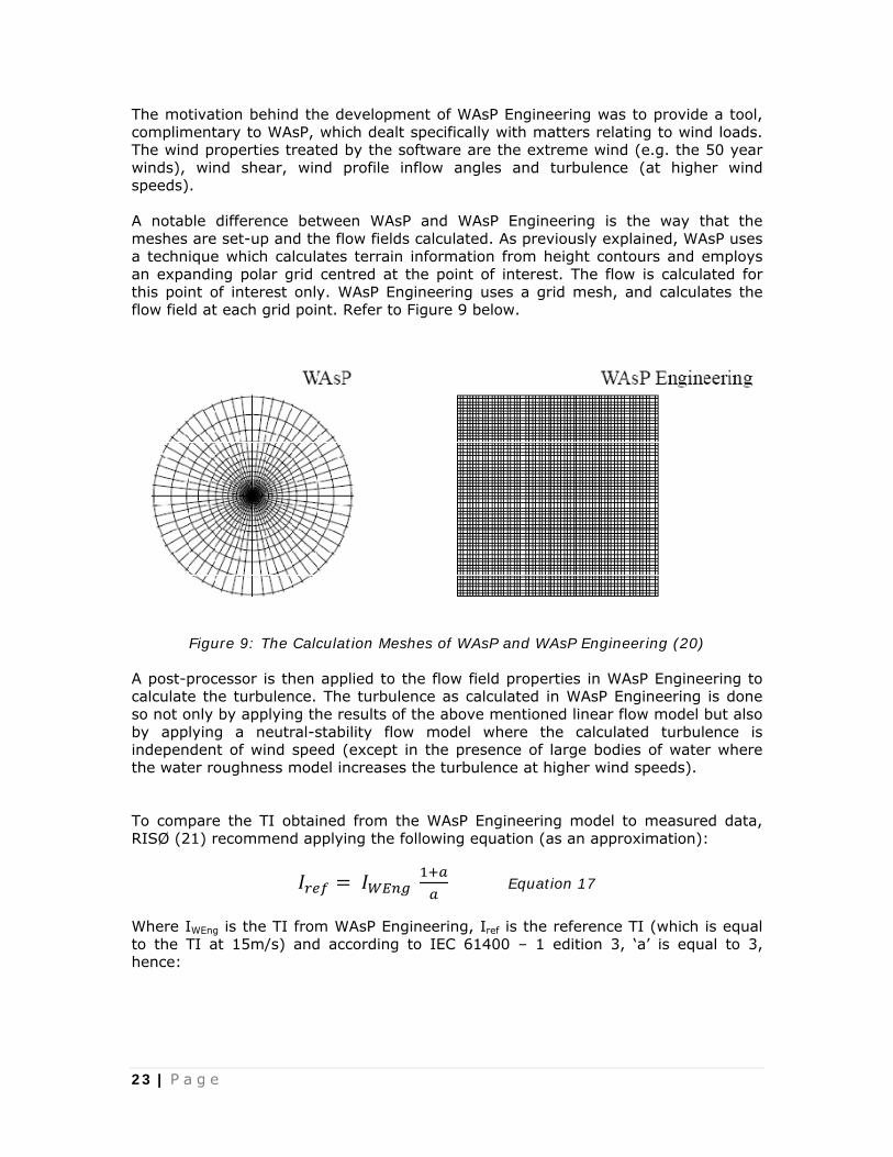
The motivation behind the development of WAsP Engineering was to provide a tool, complimentary to WAsP, which dealt specifically with matters relating to wind loads. The wind properties treated by the software are the extreme wind (e.g. the 50 year winds), wind shear, wind profile inflow angles and turbulence (at higher wind speeds). A notable difference between WAsP and WAsP Engineering is the way that the meshes are set-up and the flow fields calculated. As previously explained, WAsP uses a technique which calculates terrain information from height contours and employs an expanding polar grid centred at the point of interest. The flow is calculated for this point of interest only. WAsP Engineering uses a grid mesh, and calculates the flow field at each grid point. Refer to Figure 9 below.

Figure 9: The Calculation Meshes of WAsP and WAsP Engineering (20) A post-processor is then applied to the flow field properties in WAsP Engineering to calculate the turbulence. The turbulence as calculated in WAsP Engineering is done so not only by applying the results of the above mentioned linear flow model but also by applying a neutral-stability flow model where the calculated turbulence is independent of wind speed (except in the presence of large bodies of water where the water roughness model increases the turbulence at higher wind speeds). To compare the TI obtained from the WAsP Engineering model to measured data, RISØ (21) recommend applying the following equation (as an approximation):

Equation 17

Where IWEng is the TI from WAsP Engineering, Iref is the reference TI (which is equal to the TI at 15m/s) and according to IEC 61400 – 1 edition 3, ‘a’ is equal to 3, hence:

  

24 | P a g e

43

 

Equation 18

4 Project Aim Primarily this is a project based on validating the WindSim CFD software used for calculating wind speed, turbulence and inflow angles in complex terrain sites which exceed WAsP calculation specifications (slopes exceeding 17 degrees). Additional to this, it is desired to quantify the results of the WindSim model using different input parameters so a greater understanding of how the WindSim model operates can be achieved. It is also desired to understand how the WindSim model compares against the current industry standard tools of WAsP (utilising RIX corrections) and WAsP Engineering results and so results of the models will be compared against measured parameters. In addition to the above testing of WindSim, it is intended that this project will provide preliminary insight into CFD software and to share the information gained from this study within Suzlon and with companies who provided the data sets for this study.

5 Methodology

5.1 Data Each site used had a prerequisite of having at least 2 measurement masts (and preferably more), with each of the onsite masts ideally having at least 6 full months of high quality concurrent data. For wind resource estimates, a minimum of 12 full months is a requirement to encompass the full range of seasons in the wind data, however as this study is comparing concurrent data sets, 6 full months of 10 minute averaged data should be a suitable minimum to ensure sufficient data in relevant bins exist to develop a meaningful correlation. This is mostly achieved with the four data sets used in this study (two of the data sets are a few days short of a full 6 calendar months). Using less than 12 full months of data may however have implications on the assumption of a neutrally stratified atmosphere. Part of this assumption is intended to approximate average annual conditions and so using data from a part of the seasonal cycle may violate this assumption. As the software developer of WindSim recommends using mast data of at least 40m in height, each mast had to be at least 40m high with high quality calibrated monitoring equipment. Masts which had ultrasonic sensors attached were able to be used for validation of inflow angles calculated by the software. Each site used was required to have slopes near at least one of the masts that exceeded 17 degrees.

25 | P a g e

A summary of the data which was required for this purpose includes:

• High quality height contour data (5m contour data was used on the site itself and 10m to 20m contour data for the surrounding area (for a distance of ~ 15km from site)).

• Site photographs, Aerial photographs of the site and additional site information for building site roughness models. A site visit to each site was carried out.

• Detailed information on the measurement masts used at each site, including calibration certificates for calibrated instrumentation and mast installation reports. This included an onsite audit of all masts used in this study.

• 10 minute averages for the wind speed, standard deviation of the wind speed (from which turbulence could be calculated) and Wind direction.

• Where available, inflow angle data from ultrasonic sensors, sampled as 10 minute averages.

Thus, the participating developers were not required to provide anything other than the information they already had available for the proposed wind farms.

5.2 Validation As set out in section 3.4, mean wind speeds have been validated by comparing the fitted Weibull values between the averaged measured values and the Transferred Climatologies (as calculated in the Objects module). Wind speed frequencies for each sector are validated in much the same way. Validation of TI and inflow angles has been done through comparing the averaged measured values to the numerical results outputted from the Energy module (TI values were corrected where appropriate according to Equation 18). The calculation of wind speeds at different heights is important, and this has been tested by comparing the accuracy of the model to predict the different heights of the masts used. Due to the commercially sensitive nature of the mean wind speeds and other site climatic parameters, the results, apart from the inflow angle results, have been provided in a percentage error format (100 x (Parameterpredicted – Parametermeasured)/Parametermeasured). This format works well for the mean wind speed error (as mean wind speeds generally lie somewhere between 5m/s and 15m/s) however when it comes to presenting the errors for the TI and wind speed frequencies in this manner, some of the relevance of the result can be lost (e.g. the difference between the frequency of fmeasured=0.03 and fpredicted=0.06 is very little but as a percentage difference is high). The inflow angles have been presented as the actual error (Parameterpredicted – Parametermeasured). This is due to the generally low values this data takes and so to be a better representation of the errors. Obviously it would be ideal to present the data showing absolute and percentage differences. However these values are somewhat put into context when comparing with WAsP and WAsP Engineering results.

5.3 Hardware As WindSim is highly computationally intensive, in order to run a model of any practical size, a dedicated, high end computer is recommended. A 64-bit computer was procured for this purpose with the following specifications: Intel(R) Core(TM)2

26 | P a g e

Quad CPU, 2.93GHz processor, 4.00GB Ram. The operating system on this computer is Windows XP 64 bit edition. Significant time and effort went into configuring the required software onto the 64 bit operating platform.

5.4 Software A WindSim license was required for this study. This has been procured by Victoria University as an academic license under an agreement between the university and the software developer, but paid for by Suzlon Energy Australia PTY LTD (SEA). This license will be used exclusively for this study and must not be used for commercial applications. SEA has current commercial versions of WAsP and WAsP Engineering software to use in this study.

6 Test Sites The WindSim validation study was carried out using data from two sites. Limited information about these sites has been provided in this report as the data and information relating to these sites is commercially sensitive. As such the two sites have been nominally referred to as Site A and Site B. The names of the masts at these sites have also been modified where necessary in order to maintain anonymity of these sites. The two sites, for reasons explained below, were each divided into two separate test cases which gave four test cases overall. Throughout the rest of the report, these are generally referred to as individual sites. The model resolution of these test sites vary slightly due to the required area to encapsulate all masts included in the test and the upper limit of nodes determined by the limitations of the computer hardware (refer to section 8.1.2).

6.1 Site A Site A is an inland site based on a long running northeast-southwest mountain range with several spurs running off this main spine especially towards the south end of the site where there are branches out to the west. The site is of high complexity terrain with steep slopes and complicated gully systems and varying roughness with farm land used for sheep and cattle grazing, plantation forest and native forest. The surrounding area is of moderate to high roughness with a plateau to both the east and west and a maximum height elevation of more than 500m in comparison to the plateaus. Site A has data available from five masts with 10 minute averaged data and two of these masts are equipped with ultrasonic sensors which provide data relating to inflow angles. Four of the five masts are of 60m height and there is one 80m mast. Two of the five masts do not have any overlapping data. Because of the variable data availability, Site A has been broken into two separate test cases to make the most of the 5 masts and still maintain concurrent data periods of at least 6 months.

6.2 Site B Site B is a large coastal site located on several hill formations with smaller ridges spreading out from these. The site has steep slopes with often abrupt edges of these

27 | P a g e

slopes to plateau areas or narrow ridges. This is particularly evident along the coast where there are steep slopes of approximately 30-40 degrees mixed with areas of vertical cliffs formed due to erosion by the sea. There are also areas of cliffs on the edges of the valleys further inland in the northern part of the site, typical of the limestone country evident at the site. Site B has a moderate to high roughness with the land use being a mixture of farmland used for sheep and cattle grazing and forestry, both native and plantation. The site contains six masts recording 10 minute averaged data and has a single mast with data available from an ultrasonic sensor. A very large area separates the two furtherest most masts from each other. Given the limitations of the current hardware (4GB of Ram) to handle large models of sufficient resolution, it was most practical to treat this as two separate sites for the purposes of this validation study with a split of three masts per sub-site (North and South).

6.3 Data Sets For the purpose of software validation, it was required that all data sets used were concurrent and prepared so that should any of the sets of data in a particular group have a gap, the same period of data was required to be omitted from the adjacent data sets in the same group. The associated RIX value is also given for each mast as defined by the settings set out in section 8.1.1.

6.3.1 Site A 

6.3.1.1 Site A ‐ 01  The first data set for Site A was chosen as Mast 03, Mast 09 and Mast 11, covering the period from 11/05/2006 to 15/01/2007. The data availability for this concurrent data set is 92%. The available data sets for each mast which were selected are as follows: 03-60m: Wind speed and wind direction available from Mast 03 and instruments at 60m AGL (above ground level) (RISØ anemometer used). The RIX value for the 03 mast is 35.6. 09-80m: Wind speed and wind direction available from Mast 09 and instruments at 80m AGL (RISØ anemometer used). The RIX value for the 09 mast is 31.1. 09-60m: Wind speed and wind direction available from Mast 09 and instruments at 60m AGL (RISØ anemometer used). 09-45m: Wind speed and wind direction available from Mast 09. Wind speed is taken from the anemometer at 45m AGL (RISØ anemometer used) with the wind direction data taken from the 60m wind vane. 11-60m: Wind speed and wind direction available from Mast 11 and instruments at 60m AGL (RISØ anemometer used). The RIX value for the 11 mast is 24.8.

28 | P a g e

11-45m: Wind speed and wind direction available from Mast 11. Wind speed is taken from the anemometer at 45m AGL (RISØ anemometer used) with the wind direction data taken from the 60m wind vane.

6.3.1.2 Site A ‐ 02 The second data set for Site A was chosen as Mast 07, Mast 09, Mast 10 and Mast 11, covering the period from 07/02/2007 to 02/08/2007. The data availability for this concurrent data set is 100%. The available data sets for each mast which were selected are as follows: 07-60m: Wind speed and wind direction available from Mast 07 and instruments at 60m AGL (RISØ anemometer used). The RIX value for the 07 mast is 27.0. 07-45m: Wind speed and wind direction available from Mast 07. Wind speed is taken from the anemometer at 45m AGL (RISØ anemometer used) with the wind direction data taken from the 60m wind vane. 09-80m: Wind speed and wind direction available from Mast 09 and instruments at 80m AGL (RISØ anemometer used). 09-60m: Wind speed and wind direction available from Mast 09 and instruments at 60m AGL (RISØ anemometer used). 09-45m: Wind speed and wind direction available from Mast 09. Wind speed is taken from the anemometer at 45m AGL (RISØ anemometer used) with the wind direction data taken from the 60m wind vane. 10-60m: Wind speed and wind direction available from Mast 10 and instruments at 60m AGL (RISØ anemometer used). The RIX value for the 11 mast is 36.9. 10-45m: Wind speed and wind direction available from Mast 10 and instruments at 45m AGL (RISØ anemometer used). 11-60m: Wind speed and wind direction available from Mast 11 and instruments at 60m AGL (RISØ anemometer used). 11-45m: Wind speed and wind direction available from Mast 11. Wind speed is taken from the anemometer at 45m AGL (RISØ anemometer used) with the wind direction data taken from the 60m wind vane.

6.3.2 Site B 

6.3.2.1 Site B ‐ 01 (North) The first data set for Site B was chosen as the V, U and W masts, covering the period from 08/05/2007 to 13/12/2007. The data availability for this concurrent data set is 97%. The available data sets for each mast which were selected are as follows: V41.5m: Wind speed and wind direction available from the V mast and instruments at 41.5m AGL (NRG anemometer used). The RIX value for the V mast is 26.2.

29 | P a g e

U59m: Wind speed and wind direction available from the U mast. Wind speed is taken from the anemometer at 59m AGL (RISØ anemometer used) with the wind direction data taken from the 56.5m wind vane. The RIX value for the U mast is 21.6. U50m: Wind speed and wind direction available from the U mast. Wind speed is taken from the anemometer at 50m AGL (NRG anemometer used) with the wind direction data taken from the 56.5m wind vane. U40m: Wind speed and wind direction available from the U mast and instruments at 40m AGL (NRG anemometer used). W59m: Wind speed and wind direction available from the W mast. Wind speed is taken from the anemometer at 59m AGL (RISØ anemometer used) with the wind direction data taken from the 56.5m wind vane. The RIX value for the W mast is 18.5. W50m: Wind speed and wind direction available from the W mast. Wind speed is taken from the anemometer at 50m AGL (NRG anemometer used) with the wind direction data taken from the 56.5m wind vane. W40m: Wind speed and wind direction available from the W mast and instruments at 40m AGL (NRG anemometer used).

6.3.2.2 Site B – 02 (South)  The second data set for Site B was chosen as the X, Y and Z masts, covering the period from 05/05/2007 to 03/11/2007. This data set was restricted to the month of November due to instrument failures at the Y mast. The 60m level and the 40m level of these masts failed earlier so these were not used. The 59m RISØ anemometer on the Z mast had issues in recording higher wind data (~>15m/s) and so this also was excluded from use here. The data availability for this concurrent data set is 95%. The available data sets for each mast which were selected are as follows: X59m: Wind speed and wind direction available from the X mast. Wind speed is taken from the anemometer at 59m AGL (RISØ anemometer used) with the wind direction data taken from the 56.5m wind vane. The RIX value for the X mast is 11.1. X50m: Wind speed and wind direction available from the X mast. Wind speed is taken from the anemometer at 50m AGL (NRG anemometer used) with the wind direction data taken from the 56.5m wind vane. X40m: Wind speed and wind direction available from the X mast and instruments at 40m AGL (NRG anemometer used). Y50m: Wind speed and wind direction available from the Y mast and instruments at 50m AGL (NRG anemometer used). The RIX value for the Y mast is 13.1. Z50m: Wind speed and wind direction available from the Z mast. Wind speed is taken from the anemometer at 50m AGL (NRG anemometer used) with the wind

30 | P a g e

direction data taken from the 56.5m wind vane. The RIX value for the Z mast is 12.0. Z40m: Wind speed and wind direction available from the Z mast and instruments at 40m AGL (NRG anemometer used).

7 WindSim Sensitivity Analysis The first part of the study entailed testing the different parameters of the software and their effect on the outputs. The WindSim software has a range of parameters and it was required to do a brief investigation into what effect some of the more important parameters had on the results. This was achieved by starting with a default set of parameters and by changing just one parameter per test, it could be compared against the default baseline case to gauge if an improvement had been achieved in the model. Due to time constraints and each test run having three nested cases, it was not possible to test all parameters nor to test them comprehensively with different sites and data sets. This initial study was dubbed the “Sensitivity Analysis”. The results of the Sensitivity Analysis were noted and incorporated into the final test runs for Site A – 01, Site A – 02, Site B – 01 and Site B – 02. A potential problem with this approach may be that by testing parameters for Site A – 01, the model has been tuned specifically for Site A conditions, which may not necessarily carry over to Site B. For the purposes of the Sensitivity Analysis, part of the Site A – 01 data set was used and is described above in section 6.3.1.1

7.1 Test Parameters The following sections describe each test case of the sensitivity analysis and the parameters that were tested.

7.1.1 Test 1: Baseline Test Parameters  The baseline test as used in the Sensitivity Analysis is defined as the test case which the other test cases trialling modified test parameters (where a single parameter was changed from this baseline test case) were compared to. The baseline test case, Test 1, used default WindSim parameters (11) with the exception that for the “Terrain” module, the maximum number of cells was set as 1,000,000 (the default setting is 100,000) and for the “Wind Fields” module, the number of iterations was set as 200 (the default setting is 100). Additionally, as a full “Wind Field” module run of 12 sectors and 200 iterations per sector would take between 10 and 12 hours, only 3 sectors were chosen to reduce the time involved. The predominant wind direction sectors (as defined by mast 03) of South Southeast (150), West (270) and West Northwest (300) were analysed in full (i.e. 200 iterations were run for each of these wind direction sectors). Each test scenario was run three times for different nesting scenarios. This was defined as an outer “parent model”, defined as nest1, a second model nested inside of this parent model, defined as nest2, and a third model, nested inside the second

31 | P a g e

nested model to achieve higher cell resolution, defined as nest3. This was intended to obtain sufficient resolution to test the model but this also allowed to test the models sensitivity of successively finer grid spacing (so the results of each nested run could be compared). The first test run (the parent model, nest1) had a course resolution of 135m horizontal cell spacing and covered 29.5km in the x-direction (the east-west direction) and 25km in the y-direction (the north-south direction). This model had a total of 855,414 nodes. Note as shown in Table 3 below, the total shown in the final column actually amounts to the number of nodes (not cells). As an example, with reference to the figures given in Table 3, this is calculated as (218+1) x (185+1) x (20+1) which is equal to 855,414. x y z total Grid spacing (m) 135.0 135.0 Variable - Number of cells 218 185 20 855414

Table 3: Parent model (nest1) - Grid data.

Figure 10: Sensitivity Analysis – Site A – 01 Parent model (nest1) extent (defined by

grey box), white stars indicate mast locations.

32 | P a g e

The second test run (the middle nest, nest2) had a finer resolution (though still relatively course) of 75m horizontal cell spacing and covered 11.4km in the x-direction and 15km in the y-direction. This model had a total of 646,813 nodes. x y z total Grid spacing (m) 75.0 75.0 Variable - Number of cells 152 201 20 645813

Table 4: Middle nest (nest2) - Grid data.

Figure 11: Sensitivity Analysis - Site A – 01 middle nest (nest2) extent (defined by

grey box), white stars indicate mast locations.

33 | P a g e

The third and final test run (the inner nest, nest3) had a finer resolution (though still relatively course) of 45m horizontal cell spacing and covered 6.5km in the x-direction and 7.5km in the y-direction. This model had a total of 508,515 nodes. x y z total Grid spacing (m) 45.0 45.0 Variable - Number of cells 145 168 20 508515 Table 5: Inner nest (nest3) - Grid data.

Figure 12: Sensitivity Analysis - Site A – 01 inner nest (nest3) extent (defined by

grey box), white stars indicate mast locations.  

34 | P a g e

7.1.2 Test 2: Coupled vs Segregated solver  The Windsim software solves the non-linear steady state Reynolds Averaged Navier-Stokes equations iteratively starting with initial conditions which are guessed estimations. The user defines how many iterations are to be calculated and convergence is monitored from viewing the values of the flow parameters at a spot point (user defined with the default location in the middle of the model) and by monitoring the residual errors of the numerical simulation. The field variables that are solved are Pressure, Velocity (u, v and w), Turbulent Kinetic Energy and the Turbulent Dissipation Rate. Due to historical reasons relating to computer power, the first algorithms used in CFD were very simple to limit the demand on computer memory. These algorithms were based on the segregation of the momentum and continuity equations (refer to sections 3.1.1, 12.3.1 and 12.3.2). This historical approach is what the “Segregated” solver (SIMPLEST) is based on, and this is an iterative solving option in WindSim. A downside to the “Segregated” solver is that it can encounter issues converging when large numbers of cells are used. The “Coupled” solver (MIGAL) uses a velocity-pressure coupling technique and a “whole-field” linear solver which simultaneously updates the velocity and pressure fields in the entire domain. As it is only a linear algebraic solver it does the first part of the velocity-pressure iteration. Once this stage is complete, the background calculation engine PHOENICS completes the non-linear part of the iteration. The storage of the coefficients of the coupled equations along with the storage required for the multi-grid procedure requires much more memory than the “segregated” solver, however modern computing ability is becoming more accommodating in this respect (22). The default iterative solver in the “Wind Fields” module is the “Coupled” solver (preferred by the WindSim developer). Test 2 used the “Segregated” solver with the results compared against the results of using the “Coupled” solver in Test 1. One of the reasons that the “Coupled” solver is preferred by the developer is that the required number of iterations to achieve a converged result is significantly less than the segregated solver. 600 iterations were required in order to achieve a converged solution using the “Segregated” solver. No other parameters were changed from the baseline test run.

7.1.3 Test 3: Turbulence Model – Standard k­epsilon vs Modified  The default Turbulence model in the “Wind Fields” module is the “Standard k-epsilon” model. This was tested against the results of using the “Modified” turbulence model in Test 3. Refer to section 3.3.5 for more information about these turbulence models.  

35 | P a g e

7.1.4 Test 4: Forest vs No Forest  There are a number of areas of plantation pine forest at Site A which presented a good opportunity to test the “Forest” feature of the WindSim software. This was done in Test 4. Forests present many problems to today’s current wind software models due to the complex dynamics involved in how they initiate anomalies in the wind field which includes reduced wind speeds, increased wind shear and increased turbulence (23). A forest in WindSim can be modelled two main ways. The first is by assigning a higher roughness height to the associated areas (commonly a roughness class of 3.0 or roughness length of 0.4m is used for pine forests), which is the same way that the WAsP software models forests (though certain “fudging” of the WAsP model to accommodate some of the real life effects of forest which the model does not capture is common place (24)). The other method involves treating the forest more like an obstacle rather than a roughness through use of a canopy model. The canopy model is solved by applying a porosity value to the obstacle and the introduction of two drag forces (which act as sinks of momentum). The porosity is easy enough to visualise and a value of 0 (fully open area) to 1 (fully blocked area) is defined by the user. A porosity of 0.5 was used for testing. This may have been slightly low for a pine plantation, however attempts at testing a higher porosity were hindered by the models inability to converge at higher porosity values. The introduction of higher cell numbers appeared to aid in convergence however this was not actively pursued as a cell count of 1 million cells was desired to be maintained for consistency. However this is an area for potential future testing. The momentum sink introduced by the two drag terms present an additional term in the RANS momentum equation. Refer to Figure 13 below. The drag force coefficients, C1 and C2, which define the resistive force of the canopy are user defined, but the default of 0.01 for both coefficients were used. A forest height is also user defined, with a height of 25m used to model the onsite forest (which was mainly mature pine). The other defined parameter is the number of Z cell counts captured within the canopy height, where the default value of 3 was used. WindSim can load the areas to be treated as forest either directly through the .gws file (not pursued in the course of this study), or by associating forest with a certain roughness length. The latter was chosen for this test, with a forest being assigned to all areas with a roughness length of 0.4m. Refer to Figure 14 and Figure 15 below.

36 | P a g e

Figure 13: Additional term in RANS momentum equations resulting from Canopy

model (25)

Figure 14: Test4 outer nest Roughness and Forest map. Forest represented by grey

areas.

37 | P a g e

Figure 15: A profile section of Test4 outer nest Roughness and Forest map. Forest represented by grey areas. In this view it is possible to see the physical “height”

associated with the canopy model.

7.1.5 Test 5: Terrain Smoothing vs No Terrain Smoothing  Terrain smoothing is a feature in WindSim which allows abrupt changes in the inclination between adjacent cells to be smoothed for reasons of convergence. The reasoning behind this is that the model may not be able to converge in areas of abrupt changes (narrow valleys or sharp mountain peaks), and may instead diverge. Mathematically, changes in inclination are represented by the second order derivatives of the height. If the second order derivatives are higher than a set limit of 0.005, then a warning is displayed to the user via the “Processing Output” box when the “Terrain” module is run. The user can set a smoothing limit (0.004 is recommended by the WindSim developer) and the smoothing takes place until the second order derivatives of the height are reduced to less than the smoothing limit. This must obviously be used with caution as you are changing the height data of your model. A result of the difference in elevation of the original and smoothed terrain is given which can be checked to ensure areas of interest are not changed significantly. Refer to Figure 16 below. An alternative to Terrain Smoothing is to orthoganalise the grid (although this is documented as being the solution to modelling terrain with high inclination angles (as opposed to high second order derivatives), it appears to be a very similar concept). Making the grid orthogonal means that the grid will extend in a vertical direction along a curved line while always trying to be perpendicular to the ground (as opposed to extending in the vertical direction along straight horizontal lines).

38 | P a g e

This feature was not tested, however it is recommended that testing of this feature is included in any potential future WindSim studies. For this Test, two smoothing limits were trialled with Test5 having a smoothing limit of 0.01 and Test 5a having a smoothing limit of 0.004. The baseline test, Test 1 did not use any smoothing.

Figure 16: Digital Terrain Model Test 5 nest 3 – Delta elevation [m]. Areas with

second order derivatives above given limit (0.01) have been smoothed. The above plot displays the difference in elevation between the original and smoothed terrain.

39 |

7.1.6 The maxiand tthe h(whic Due tunab The ohad a Grid sNumb

The horiz Grid sNumb

7.2 The rmean

7.2.1 The scenafrom site),energenergand espeed

P a g e

6 Test 6: N

number of mum numbthe purposehorizontal och is what T

to a model ble to be run

outer nest ha total of 86

spacing (m) ber of cells

middle nesontal cell sp

spacing (m) ber of cells

Results

results of thn wind spee

1 Wind sp

mean windarios model both a load, and from gy predictiogy and reveenergy, withd.

 Number of

cells that ber of 1,000e of Test 6 wor the verticTest 1 used)

failure (pern.

had a cours62,920 node

Tabl

st had a fipacing. This

Table

he Sensitivitd and turbu

peeds 

speed reslled the winds case (ma an econom

on a small eenue predicth the energy

f cells in Z

the model 0,000 cells was to see cal. The def. Test 6 was

haps failure

se resolutioes.

x 210.0 140

le 6: Test 6,

ner resolut model had

x 105.0 109

e 7: Test 6,

ty analysis wulence.

ults were and flow. Accaking sure tmical point error in windtions. This iy content in

Z Direction

has affectwas used tif the “limitefault numbes done usin

e to converg

n of 210m

y 210.0 119

, outer nest

tion (though a total of 7

y 105.0 143

middle nes

were analys

a vital indiccurately prethe correct of view in

d speed preis due to thn the wind p

n. 

ts the resothroughout ed” cell numer of cells ig 50 cells in

ge), the fina

horizontal c

z Variab

50 t - Grid data

h still relat794,937 nod

z Variabl

50

st - Grid data

sed using tw

cator as to edicting winclass of tur terms of eedictions canhe relationshproportional

lution of th the Sensitimber was bein the Z dirn the vertica

l inner nest

cell spacing

tole

862a.

tively coursdes.

toe

794

ta.

wo different

how the dd speeds a

rbine is empenergy predn lead to lahip between to the cube

he model. vity analysest served irection is 2al direction.

ted layer wa

. This mode

otal -

2920

se) of 105m

otal -

4937

parameters

different Tesre importanployed at thdiction. Witrge errors i

n wind speee of the win

A is in

20

as

el

m

s,

st nt he th in ed nd

40 | P a g e

For the wind speed analysis, a single level from each of the three masts of the Site A – 01 data case were viewed (03_60m, 09_80m and 11_60m), each cross predicting the other two. For a full set of results, see Table 30 to Table 36 in Appendix 12.1.1. From Table 8 below, which shows the relationship between the cross predictions of the three masts analysed, a few general conclusions can be drawn about how these cross-predicted each other. The main feature of these results can be seen that any cross prediction involving the 80m mast with the two 60m masts model poorly when compared to the cross predictions between the two 60m masts. In particular the cross predictions involving the 80m mast with any of the other two 60m masts for the 270 degree direction sector are very poor (43% average absolute error). A general conclusion can be drawn that the model does not appear to be calculating the wind profile correctly and hence the height extrapolation of wind data is not as successful as the horizontal, refer to section 8.4 for more on height extrapolation.

Predicted Reference sector All Tests All Sectors

03_60m

09_80m 150 5%

15% 270 25% 300 14%

11_60m 150 20%

9% 270 4% 300 4%

09_80m

03_60m 150 5%

26% 270 58% 300 14%

11_60m 150 16%

29% 270 55% 300 16%

11_60m

03_60m 150 12%

7% 270 3% 300 5%

09_80m 150 9%

21% 270 34% 300 21%

Table 8: Sensitivity Analysis Wind Speed results – Average of absolute percentage difference between measured and predicted results of all tests for each mast and

sector.

Now looking more specifically at the different test cases for wind speed prediction, the summarised results are given below in Table 9. The results are given as averages of the absolute values of the prediction errors for each nest case of each test and also the overall average of that test (the overall test average does not apply to test 6 as only two nesting cases were possible to run for this (refer section 7.1.6)). Test 4, the forest canopy model, obviously did not work well. This is not to say that after a single nested test case by an inexperienced CFD user that there is no merit in the forest canopy model (actually the forest model returned the best results for cross-prediction between the 80m mast and the two 60m mast for the poorly performing 270 degree sector), only that in this case, generally speaking, it did not

41 | P a g e

work out well and this was enough of a deterrent not to use this feature in the final test runs. Apart from the forest model test case (and the aforementioned case of the 270 sector involving the 80m mast), all of the other test cases resulted in a close cluster of wind speed results, showing that the sensitivity of the wind speeds to the majority of the tested parameters appears to be low. Overall, it was the standard test case, test 1, which marginally performed the better overall. As the large errors from the 270 degree sector combined with vertical extrapolation heavily weighted the averaged results, the final column in Table 9 gives the same average of absolute errors with this component removed with similar trends as described above, but yielding lower absolute errors.

Test Definition Test no. Nest

All masts & Sectors

Mean All Nests

Excluding 09 sector 270

Baseline Test1 nest1 16%

15% 6%

nest2 15% 6% nest3 15% 7%

Segregated solver Test2

nest1 15% 16%

6% nest2 16% 7% nest3 16% 8%

Modified K-ε model Test3

nest1 16% 16%

7% nest2 15% 7% nest3 16% 7%

Forestry Test4 nest1 37%

29% 40%

nest2 25% 26% nest3 26% 27%

Smoothing 0.01 Test5

nest1 16% 16%

6% nest2 15% 6% nest3 16% 7%

Smoothing 0.004 Test5a

nest1 16% 16%

7% nest2 15% 7% nest3 15% 8%

Z cells 50 Test6 nest1 19% - 9%

nest2 16% 7% Table 9: Sensitivity Analysis Wind Speed results – Average of absolute percentage difference between measured and predicted results of all masts for each test and

each nest. In terms of how the different nesting cases performed, surprisingly (apart perhaps from Test 4) the different nests did not create as much of a refinement in accuracy as one would intuitively expect resulting from the higher resolution models. In terms of wind speeds, one can expect an incremental increase in higher accuracy for a second nested case, but as Table 10 and Table 11 show below, there is little advantage in going to a third nested case (and as can be seen in Table 9 above, often leads to higher errors). The lack of refined accuracy in the nested layers may come from inexperience on the user’s behalf, perhaps some artificial blocking effect is occurring in the model due to the steep terrain at site, or perhaps even further refinement is required. As Test 4 yielded comparatively much higher errors, this case

42 | P a g e

has been excluded from the below summary results in Table 11 which shows nest2 as the better wind speed predicting case.

Results - Nest Case Summary, excluding Test6

nest1 nest2 nest3 19% 17% 17%

Table 10: Sensitivity Analysis Wind Speed results – Average of absolute percentage difference between measured and predicted results of all masts and all tests (excluding test 6) showing overall affect of the three different nesting cases.

Results - Nest Case Summary,

excluding Test4 & Test6 nest1 nest2 nest3 16% 15% 16%

Table 11: Sensitivity Analysis Wind Speed results – Average of absolute percentage difference between measured and predicted results of all masts and all tests

(excluding test 4 and test 6) showing overall affect of the three different nesting cases.

7.2.2 Turbulence  The other main parameter tested in the Sensitivity Analysis was Turbulence. As described in section 3.3.6, The TI outputs of the WindSim model are independent of wind speed and appear to be comparable to the TI at a wind speed of 15m/s after application of Equation 18 (effectively multiplying the result by a factor of 4/3). For the Turbulence analysis, a single level from each of the 60m masts (03_60m and 11_60m) and two levels from the 80m mast (09_80m and 09_60m) were used from the Site A – 01 data set. It was the author’s initial understanding that WindSim was configured to provide TI values as a function of a referenced wind speed (with the reference wind speed defined by the speed ups between the turbine location and the boundary layer wind speed). The TI results of the Sensitivity Analysis were initially based on this assumption, comparing the actual TI output with the measured TI at the reference wind speed. After running full test runs of the four test sites at four different boundary condition inlet wind speeds, it was discovered that the TI did not change or changed negligible amounts regardless of the wind speed. It was only then discovered from correspondence with the software developer that WindSim is based on the assumption of a neutrally stable atmosphere. Under these assumptions, the TI is independent of wind speed. The software developer later recommended comparing the model outputs to measured TI values at 15m/s after applying the same correction factor that RISOE recommends for its WAsP Engineering model outputs. Effectively this means multiplying the model outputs by a factor of 4/3 before comparing these with the measured turbulence at 15m/s. Refer to sections 3.6 and 8.5 for how this was handled in the current study.

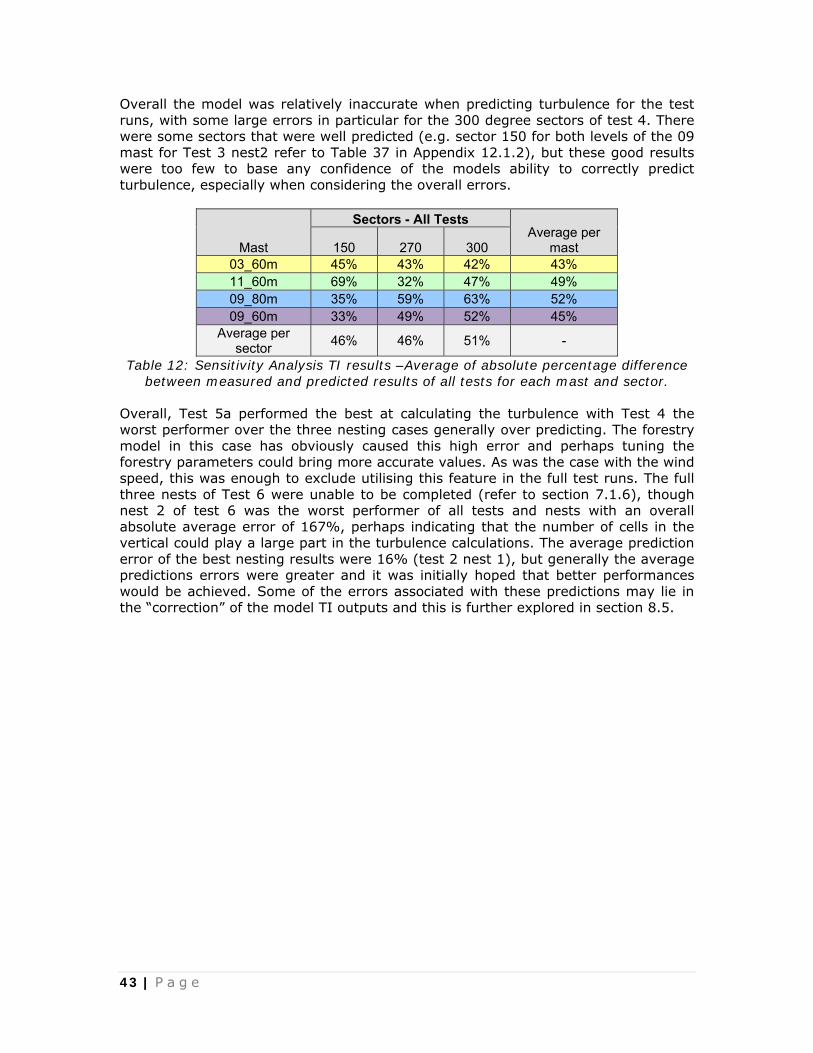
43 | P a g e

Overall the model was relatively inaccurate when predicting turbulence for the test runs, with some large errors in particular for the 300 degree sectors of test 4. There were some sectors that were well predicted (e.g. sector 150 for both levels of the 09 mast for Test 3 nest2 refer to Table 37 in Appendix 12.1.2), but these good results were too few to base any confidence of the models ability to correctly predict turbulence, especially when considering the overall errors.

Mast

Sectors - All Tests Average per

mast 150 270 300 03_60m 45% 43% 42% 43% 11_60m 69% 32% 47% 49% 09_80m 35% 59% 63% 52% 09_60m 33% 49% 52% 45%

Average per sector 46% 46% 51% -

Table 12: Sensitivity Analysis TI results –Average of absolute percentage difference between measured and predicted results of all tests for each mast and sector.

Overall, Test 5a performed the best at calculating the turbulence with Test 4 the worst performer over the three nesting cases generally over predicting. The forestry model in this case has obviously caused this high error and perhaps tuning the forestry parameters could bring more accurate values. As was the case with the wind speed, this was enough to exclude utilising this feature in the full test runs. The full three nests of Test 6 were unable to be completed (refer to section 7.1.6), though nest 2 of test 6 was the worst performer of all tests and nests with an overall absolute average error of 167%, perhaps indicating that the number of cells in the vertical could play a large part in the turbulence calculations. The average prediction error of the best nesting results were 16% (test 2 nest 1), but generally the average predictions errors were greater and it was initially hoped that better performances would be achieved. Some of the errors associated with these predictions may lie in the “correction” of the model TI outputs and this is further explored in section 8.5.

44 | P a g e

Test Definition Test no. Nest

All masts & Sectors

Mean All Nests

Baseline Test1 nest1 24%

29% nest2 28% nest3 34%

Segregated solver Test2

nest1 16% 32% nest2 38%

nest3 41%

Modified K-ε model Test3

nest1 27% 30% nest2 27%

nest3 35%

Forestry Test4 nest1 147%

135% nest2 127% nest3 129%

Smoothing 0.01 Test5

nest1 24% 28% nest2 28%

nest3 31%

Smoothing 0.004 Test5a

nest1 26% 22% nest2 20%

nest3 21% Z cells

50 Test6 Nest1 72% - Nest2 167%

Table 13: Sensitivity Analysis TI results – Average of absolute percentage difference between measured and predicted results of all masts for each test and nest.

Analysing the combined results of the three nest cases, as was the case with the wind speed averages, the higher resolution obtained in the model by introducing successive nesting cases did not yield the results one would intuitively expect. These results actually show the turbulence predictions growing more inaccurate at each successive nested case, with the nest1 scenarios performing the best. This could be due to the larger models ability to capture the influence of the wider area, or it could be due to potential errors in the model becoming compounded at such a high resolution.

Results - Nest Case Summary, excluding Test6

nest1 nest2 nest3 38% 44% 47%

Table 14: Sensitivity Analysis TI results – Average of absolute percentage difference between measured and predicted results of all masts and all tests (excluding test 6)

showing overall affect of the three different nesting cases.

45 | P a g e

7.3 Conclusions from Sensitivity Analysis Overall it was clear that without further testing and understanding that the forest parameter should be omitted from the full test runs. The coupled solver tended to be the better performing of the two solver cases (Test 1 compared to Test 2) and as this resulted in greatly reduced computational time, the coupled solver was chosen over the segregated for the full test runs. As Test5a performed well for both the TI and velocity tests, smoothing was employed in the full test runs with a smoothing value of 0.004 selected. When initial testing was done, the TI results were taken as the uncorrected TI at the referenced wind speed (refer to section 3.3.6). This resulted in slightly better TI results for the modified turbulence model over the standard k-epsilon model and so the modified turbulence model was applied to the full test runs. As can be seen from the above results, the TI results of Test 3 and Test 1 do not vary significantly and so this is not a seen as a major issue for the full test run models. The lack of refined accuracy in the nest3 test cases may come from inexperience on the user’s behalf, perhaps some artificial blocking effect is occurring in the model due to the steep terrain at site, or perhaps even further refinement is required. As the nesting cases did not yield any major advantages for going from nest2 to nest3, it was decided to base the full test runs on a single nested case (nested only once as was the case for nest2). Additional to the tested parameters, it was decided to employ grid refinement to increase the resolution of the grid in the area of interest on the nested layer (refer to section 3.4.1). Also, upon conversations with an experienced WindSim user, for the purposes of accuracy, it was decided to increase the number of cells in the vertical direction. With the apparent failings of Test6, a dramatic increase was not advisable, and the number of cells in the vertical was chosen as 30 for the full test runs. It was assumed that an increase in the number of cells would be beneficial for the models (and required to accommodate the additional number of vertical cells) but there was a cell limit enforced by the hardware capabilities (mainly the amount of RAM), and 1.5 million was selected as it appeared to be the largest model size available without crashing the calculations. The wind speed and TI results of the full test runs are presented in sections 8.2, and 8.5 respectively however it is interesting to compare how the results of the equivalent mast predictions of the full test results for Site A – 01 compared with the baseline test case for the Sensitivity Analysis. From Table 15 below, it can be seen that the desired increase in accuracy was not achieved and removing the 270 degree sector for all cross predications involving the 09 mast (the 80m mast), the accuracy actually decreases.

46 | P a g e

Test Definition Test no. Nest

All masts & Sectors

Mean All Nests

Excluding 09 sector 270

Baseline Test1 nest1 16%

15% 6%

nest2 15% 6% nest3 15% 7%

Full Test Site A - 01 nest2 15% - 8% Table 15: Full test results of mean wind speed from Site A – 01 vs the baseline test

case results of mean wind speed from the Sensitivity Analysis (using equivalent mast predictions)

As for the Turbulence, it can be seen from below that the accuracy in predicting the turbulence at the equivalent masts (09_80, 09_60, 03_60 and 11_60) for the equivalent sectors (SSE, W and WNW) was similar but slightly less accurate for the nest2 case for the baseline tests. Overall, it can be concluded that the desired accuracy was not achieved from applying the results of the Sensitivity Analysis to the full test runs.

Test Definition Test Nest

All masts & Sectors

All Nests

Baseline Test1 nest1 24%

29% nest2 28% nest3 34%

Full Test Site A - 01 nest2 29% - Table 16: Full test results of TI from Site A – 01 vs the baseline test case results of

TI from the Sensitivity Analysis (using equivalent mast predictions)

8 Full Test results The assumptions and associated parameter settings from the Sensitivity Analysis were applied to the Full test runs to yield wind speed, TI and inflow outputs at the referenced mast locations for the four sites. These results were compared to the measured parameters which illustrated the accuracy of the model in predicting these parameters. Further, the same base inputs used in the WindSim models were used in the WAsP and WAsP Engineering models with the results compared to WindSim to gauge the comparative accuracy of the two types of models over the four sites. The default settings of these two linear models were used for simplicity, however it is possible to alter or “tune” these models to specific sites to achieve higher accuracy in the results. Additionally a brief comment on the definition of sectors as they relate to each piece of software. Both WindSim and WAsP Engineering define the results per sector as the path at the centre of the sector (so for the eastern sector, this would be for a narrow path at 90 degrees). WAsP defines results in terms of the average of the sector. For this reason, using smaller sectors would be better for directly comparing WindSim and WAsP outputs, however due to calculation times involved in running WindSim, 30 degree sectors have been chosen.

47 | P a g e

The WindSim model was run for four different Boundary Condition inlet wind speeds. These were 5m/s, 10m/s, 15m/s and 20m/s. Negligible changes in the predicted wind speeds were found for all four sites (refer to Table 17 below) and so the data presented here is based on the models with an inlet wind speed of 10m/s.

Site A - 01 Site A - 02 Site B - 01 Site B - 02 Average difference between max and min predicted mean wind speeds for the four inlet wind speeds (5, 10, 15 & 20 m/s)

0.6% 0.3% 0.3% 0.4%

Table 17: Average difference in mean wind speed predictions for all cross predictions for all four inlet test conditions. The difference is calculated as the percentage

difference between the max and min predicted wind speeds as defined by the inlet wind speed test case at each cross prediction case for each site.

The wind speed values derived from WAsP were further analysed to gauge the effect of “correcting” the outputs based on the delta RIX methodology (refer to section 3.5.1). The delta RIX settings are defined below.

8.1.1 Delta RIX settings  The RIX set-up was based on the default WindPRO settings. The RIX set up is a topic of open debate within the industry, however this topic is outside of the scope of the current project, and as such default values were selected for simplicity. These default values were:

• Radius for RIX calculation: 3500m • Directional step: 5o • Steepness threshold: 30.0% • Directional weight controlled by: Equally distributed

8.1.2 Model Grid Spacing  The grid spacing’s shown from Table 18 to Table 21 were achieved for the four nested models. It is evident that in such complex terrain that the grid spacing achieved was much less than desirable and this is seen as a notable shortcoming of the tests. A resolution of at least 10m would be preferable in such complex terrain and even finer if possible. This was not able to be achieved due to the limitations of the hardware and the required area to be finely modelled which captured all cross predicting masts. A nodal count of 10 million would have been required to get near a resolution of 10m for the tested modal areas. Other techniques of transferring climatologies are a possible solution to get around this problem (when a measured location has its data transferred to another model, so the need to capture both the reference and predicted sites in the single model is not necessary) though these were not investigated over the course of this study. It is recommended that any future testing be done on a machine with much higher RAM capacity (16GB to 32GB) so as to achieve desirable resolution.

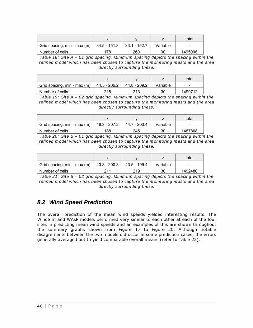
48 | P a g e

   x y z total Grid spacing, min - max (m) 34.5 - 151.8 33.1 - 152.7 Variable - Number of cells 178 260 30 1495008 Table 18: Site A – 01 grid spacing. Minimum spacing depicts the spacing within the refined model which has been chosen to capture the monitoring masts and the area

directly surrounding these.    x y z total Grid spacing, min - max (m) 44.5 - 206.2 44.8 - 209.2 Variable - Number of cells 218 213 30 1499712 Table 19: Site A – 02 grid spacing. Minimum spacing depicts the spacing within the refined model which has been chosen to capture the monitoring masts and the area

directly surrounding these.    x y z total Grid spacing, min - max (m) 46.3 - 207.2 44.7 - 203.4 Variable - Number of cells 188 245 30 1487808 Table 20: Site B – 01 grid spacing. Minimum spacing depicts the spacing within the refined model which has been chosen to capture the monitoring masts and the area

directly surrounding these.    x y z total

Grid spacing, min - max (m) 43.8 - 200.3 43.5 - 199.4 Variable - Number of cells 211 219 30 1492480 Table 21: Site B – 02 grid spacing. Minimum spacing depicts the spacing within the refined model which has been chosen to capture the monitoring masts and the area

directly surrounding these.

8.2 Wind Speed Prediction The overall prediction of the mean wind speeds yielded interesting results. The WindSim and WAsP models performed very similar to each other at each of the four sites in predicting mean wind speeds and an examples of this are shown throughout the summary graphs shown from Figure 17 to Figure 20. Although notable disagrements between the two models did occur in some prediction cases, the errors generally averaged out to yield comparable overall means (refer to Table 22).

49 | P a g e

Figure 17: Model errors for mean velocity for Site A - 01 for both the WindSim and

WAsP models. The horizontal scale represents each of the 20 cross predictions. Model errors are defined as 100 x (Upredicted – Umeasured)/Umeasured.

Figure 18: Model errors for mean velocity for Site A - 02 for both the WindSim and

WAsP models. The horizontal scale represents each of the 20 cross predictions. Model errors are defined as 100 x (Upredicted – Umeasured)/Umeasured.

‐8.0%

‐6.0%

‐4.0%

‐2.0%

0.0%

2.0%

4.0%

6.0%

8.0%

03_60m

_to_

09_45m

 

03_60m

_to_

09_60m

 

03_60m

_to_

09_80m

 

03_60m

_to_

11_45m

 

03_60m

_to_

11_60m

 

09_80m

_to_

03_60m

 

09_80m

_to_

11_60m

 

09_80m

_to_

11_45m

 

09_80m

_to_

09_60m

 

09_80m

_to_

09_45m

 

11_60m

_to_

03_60m

 

11_60m

_to_

09_45m

 

11_60m

_to_

09_60m

 

11_60m

_to_

09_80m

 

11_60m

_to_

11_45m

 

09_60m

_to_

03_60m

 

09_60m

_to_

11_45m

 

09_60m

_to_

11_60m

 

09_45m

_to_

11_60m

 

11_45m

_to_

09_80m

 

% Error of p

redicted

 mean wind speed

Site A ‐ 01WindSim vs WAsP ‐Model errors for mean velocity 

WindSim

WAsP

‐15.0%

‐10.0%

‐5.0%

0.0%

5.0%

10.0%

15.0%

07_60m

_to_

07_45m

 

07_60m

_to_

09_45m

 

07_60m

_to_

09_60m

 

07_60m

_to_

09_80m

 

07_60m

_to_

10_45m

 

07_60m

_to_

10_60m

 

07_60m

_to_

11_45m

 

07_60m

_to_

11_60m

 

10_60m

_to_

10_45m

 

10_60m

_to_

07_45m

 

10_60m

_to_

07_60m

 

10_60m

_to_

09_45m

 

10_60m

_to_

09_60m

 

10_60m

_to_

09_80m

 

10_60m

_to_

11_45m

 

10_60m

_to_

11_60m

 

07_45m

_to_

09_80m

 

10_45m

_to_

09_80m

 

07_45m

_to_

10_60m

 

07_45m

_to_

11_60m

 

% Error of p

redicted

 mean wind speed

Site A ‐ 02 WindSim vs WAsP ‐Model errors for mean velocity 

WindSim

WAsP

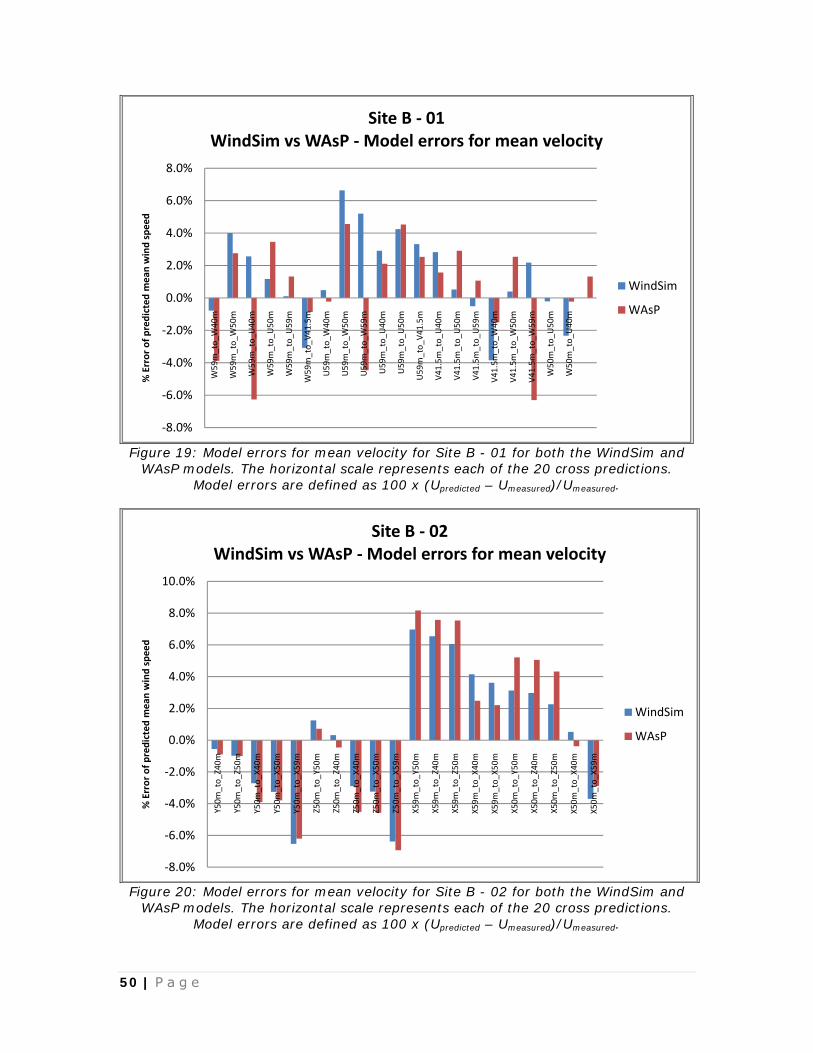
50 | P a g e

Figure 19: Model errors for mean velocity for Site B - 01 for both the WindSim and

WAsP models. The horizontal scale represents each of the 20 cross predictions. Model errors are defined as 100 x (Upredicted – Umeasured)/Umeasured.

Figure 20: Model errors for mean velocity for Site B - 02 for both the WindSim and

WAsP models. The horizontal scale represents each of the 20 cross predictions. Model errors are defined as 100 x (Upredicted – Umeasured)/Umeasured.

‐8.0%

‐6.0%

‐4.0%

‐2.0%

0.0%

2.0%

4.0%

6.0%

8.0%

W59m_to_

W40m 

W59m_to_

W50m 

W59m_to_

U40m 

W59m_to_

U50m 

W59m_to_

U59m 

W59m_to_

V41.5m

 

U59m_to_

W40m 

U59m_to_

W50m 

U59m_to_

W59m 

U59m_to_

U40m 

U59m_to_

U50m 

U59m_to_

V41.5m

 

V41.5m

_to_

U40m 

V41.5m

_to_

U50m 

V41.5m

_to_

U59m 

V41.5m

_to_

W40m 

V41.5m

_to_

W50m 

V41.5m

_to_

W59m 

W50m_to_

U50m 

W50m_to_

U40m 

% Error of p

redicted

 mean wind speed

Site B ‐ 01WindSim vs WAsP ‐Model errors for mean velocity 

WindSim

WAsP

‐8.0%

‐6.0%

‐4.0%

‐2.0%

0.0%

2.0%

4.0%

6.0%

8.0%

10.0%

Y50m

_to_

Z40m

 

Y50m

_to_

Z50m

 

Y50m

_to_

X40m

 

Y50m

_to_

X50m

 

Y50m

_to_

X59m

 

Z50m

_to_

Y50m

 

Z50m

_to_

Z40m

 

Z50m

_to_

X40m

 

Z50m

_to_

X50m

 

Z50m

_to_

X59m

 

X59m

_to_

Y50m

 

X59m

_to_

Z40m

 

X59m

_to_

Z50m

 

X59m

_to_

X40m

 

X59m

_to_

X50m

 

X50m

_to_

Y50m

 

X50m

_to_

Z40m

 

X50m

_to_

Z50m

 

X50m

_to_

X40m

 

X50m

_to_

X59m

 

% Error of p

redicted

 mean wind speed

Site B ‐ 02 WindSim vs WAsP ‐Model errors for mean velocity 

WindSim

WAsP

51 | P a g e

The total absolute average error for all mean wind speeds from the 80 cross predictions show that the WindSim model performed slightly better overall than WAsP. But generally speaking, the performance of the CFD software as applied in this study for predicting mean wind speeds did not perform significantly better than the standard (non RIX corrected) WAsP software. Refer to Table 22 below.

Mean Absolute Prediction Error Site WindSim WAsP WAsP ∆RIX

Site A - 01 2.8% 2.9% 8.0% Site A - 02 5.3% 5.1% 5.9% Site B - 01 2.4% 2.5% 6.2% Site B - 02 3.4% 3.9% 2.8% overall mean 3.5% 3.6% 5.7%

Table 22: The mean absolute prediction error for all cross-predictions at each site and as calculated by each model is provided (including WAsP with delta RIX

corrections applied, refer to section 8.3). The overall mean for each model for all 80 cross-predictions (20 per site) is also given. Model errors are defined as 100 x

(Upredicted – Umeasured)/Umeasured. The prediction of mean wind speed is a critical component in assessing potential wind farm sites. However so is assessing the frequency of winds from each direction and the mean wind speeds for each direction. This plays a large part in optimising the turbine layout of a wind farm. The WindSim and WAsP models were compared on their ability to predict the frequency of winds from each sector (in effect, how the wind changes direction from the reference site to the predicted site) and also the mean wind speed for each sector. 12 sectors of 30 degree width were used, which is a common industry sector size. The sector-wise mean wind speed prediction offers a greater insight into the detail captured by each model. If a model both over and under predicts mean wind speed for some sectors, the overall predicted mean wind speed can still be close to the actual mean. However the overall mean wind speed is not necessarily showing the wind engineer designing a wind farm the information they need to most optimally space turbines1. WindSim performed better than WAsP at predicting both frequency and mean wind speeds on a per sector basis at all four sites. Unlike the prediction of the overall mean wind speeds, this would appear to be an advantage of WindSim over WAsP. Table 23 below provides the summary data of this comparison. Interestingly it also shows that both Site A – 01 and Site A – 02 were poorly predicted by both models in this respect. Site A in general is a highly complex site, (as indicated by the associated RIX values in section 6.3), which may help explain the difference.

1 Additional to these parameters, for the purposes of calculating the expected energy from a wind turbine, the overall and sector specific wind speed distribution is important (the spread or the frequency of the different wind speed bins making up the sector specific and overall average winds). These values are depicted by the A and k Weibull factors. These parameters have not been evaluated in this study.

52 | P a g e

Model Absolute Prediction Error in predicting

parameters by sector – Mean of all sectors Model WindSim WAsP Site mean freq mean freq

Site A - 01 23.3% 67.1% 35.2% 98.1% Site A - 02 26.2% 98.7% 34.7% 110.8% Site B - 01 8.7% 13.5% 9.8% 14.4% Site B - 02 9.8% 14.4% 11.9% 14.9% overall mean 17.0% 48.4% 22.9% 59.5%

Table 23: The mean absolute errors of both models predicting frequency and mean wind on a per sector basis at each site. 30 degree sectors were used in the analysis.

Model errors are defined as 100 x (Upredicted – Umeasured)/Umeasured.

8.3 Delta Rix Corrections Delta RIX corrections were applied using the equation derived from Figure 8 (correction = WAsP Value/exp(1.508*(Delta RIX value)/100). When the delta RIX corrections were applied to the WAsP generated wind speed values, mixed results ensued. This delta RIX method when applied to the data at Site B – 02 performed better than both the WindSim model and the un-corrected WAsP results (refer to Figure 21 below). When applied to the other three test cases, however, the results were less favourable with the other two modelling methods outperforming the delta RIX method (refer to Table 22). In the case of Site A – 01 in particular, significant prediction errors occurred as a result of employing the delta RIX method. The main purpose of introducing the delta RIX method was to compare the WindSim model to current “industry standard” tools. As WAsP was expected to perform poorly in complex terrain due to it being based on a linear flow model, the delta RIX method is the best “fix” for this software currently available to the industry. Interestingly, the masts at Site B – 02 contained the lowest RIX values of all sites (refer to section 6.3). The conclusion that can be drawn here is that it is far from a perfect method and it should be used with caution. Further research is required in the application of the delta RIX correction method, which may include additional testing of a range of different sites encompassing various roughness, orographic and stability cases to further develop the delta RIX corrections.

53 | P a g e

Figure 21: Model errors for mean velocity for Site B - 02 for the WindSim, WAsP and

delta RIX corrected WAsP models. The horizontal scale represents each of the 20 cross predictions. Model errors are defined as 100 x (Upredicted – Umeasured)/Umeasured.

8.4 Prediction of different heights With the ever increasing hub heights of modern wind turbines and the high associated costs with monitoring at such high levels, more often than not, wind resource predictions are made from data measurements lower than hub height. Additionally, it is important from a loads point of view to have a good prediction of the wind shear acting across the swept area of the blades (at the upper most and lower most points). It is therefore important for the model making these predictions to be accurate in predicting the wind profile. With this in mind, the 80 cross predictions from the two sites and the four nested cases were divided into those that were cross predicting to a higher level and those that were cross predicting to a lower level. As has already been seen from the previous section, the WindSim and WAsP models behaved very similarly. As the experiment with delta RIX by and large did not return favourable results, this was not employed for this analysis. When cross predicting to a lower level, both models had more of a tendency to over predict the wind speeds. This can be seen in Figure 22 below, where the majority of the predictions resulted in positive errors. This is also reflected from the mean average as given in Table 24 which shows the overall average as slightly positive for the two models reflecting a general over prediction.

‐8.0%

‐6.0%

‐4.0%

‐2.0%

0.0%

2.0%

4.0%

6.0%

8.0%

10.0%

Y50m

_to_

Z40m

 

Y50m

_to_

Z50m

 

Y50m

_to_

X40m

 

Y50m

_to_

X50m

 

Y50m

_to_

X59m

 

Z50m

_to_

Y50m

 

Z50m

_to_

Z40m

 

Z50m

_to_

X40m

 

Z50m

_to_

X50m

 

Z50m

_to_

X59m

 

X59m

_to_

Y50m

 

X59m

_to_

Z40m

 

X59m

_to_

Z50m

 

X59m

_to_

X40m

 

X59m

_to_

X50m

 

X50m

_to_

Y50m

 

X50m

_to_

Z40m

 

X50m

_to_

Z50m

 

X50m

_to_

X40m

 

X50m

_to_

X59m

 

% Error of p

redicted

 mean wind speed

Site B ‐ 02 WindSim vs WAsP ‐Model errors for mean velocity 

WindSim

WAsP

WAsP RIX

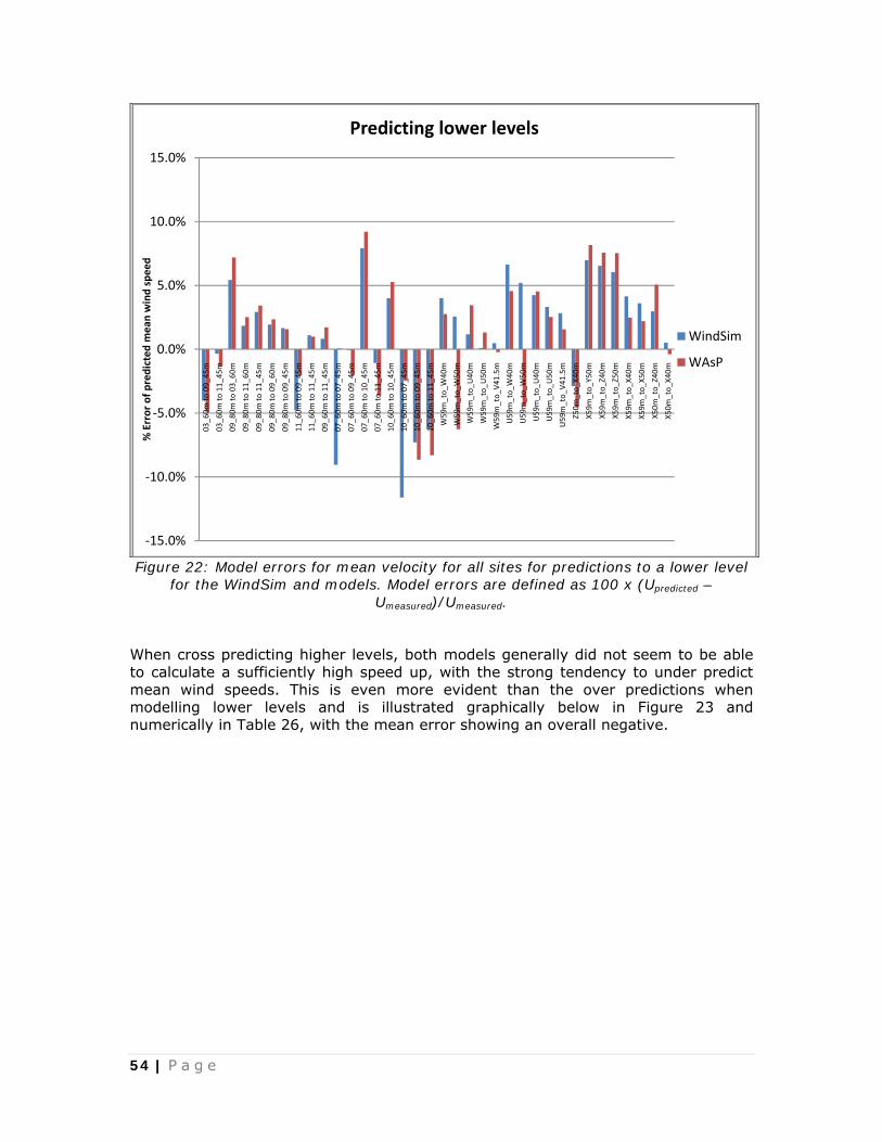
54 | P a g e

Figure 22: Model errors for mean velocity for all sites for predictions to a lower level

for the WindSim and models. Model errors are defined as 100 x (Upredicted – Umeasured)/Umeasured.

When cross predicting higher levels, both models generally did not seem to be able to calculate a sufficiently high speed up, with the strong tendency to under predict mean wind speeds. This is even more evident than the over predictions when modelling lower levels and is illustrated graphically below in Figure 23 and numerically in Table 26, with the mean error showing an overall negative.

‐15.0%

‐10.0%

‐5.0%

0.0%

5.0%

10.0%

15.0%

03_60m

 to 09_45

m 

03_60m

 to 11_45

m 

09_80m

 to 03_60

m 

09_80m

 to 11_60

m 

09_80m

 to 11_45

m 

09_80m

 to 09_60

m 

09_80m

 to 09_45

m 

11_60m

 to 09_45

m 

11_60m

 to 11_45

m 

09_60m

 to 11_45

m 

07_60m

 to 07_45

m 

07_60m

 to 09_45

m 

07_60m

 to 10_45

m 

07_60m

 to 11_45

m 

10_60m

 to 10_45

m 

10_60m

 to 07_45

m 

10_60m

 to 09_45

m 

10_60m

 to 11_45

m 

W59

m_to_

W40

m 

W59

m_to_

W50

m 

W59

m_to_

U40

m 

W59

m_to_

U50

m 

W59

m_to_

V41.5m

 

U59

m_to_

W40

m 

U59

m_to_

W50

m 

U59

m_to_

U40

m 

U59

m_to_

U50

m 

U59

m_to_

V41.5m

 

Z50m

_to_

X40m

 

X59m

_to_

Y50m

 

X59m

_to_

Z40m

 

X59m

_to_

Z50m

 

X59m

_to_

X40m

 

X59m

_to_

X50m

 

X50m

_to_

Z40m

 

X50m

_to_

X40m

 

% Error of p

redicted

 mean wind speed

Predicting lower levels

WindSim

WAsP

55 | P a g e

Figure 23: Model errors for mean velocity for all sites for predictions to a higher level

for the WindSim and WAsP models. Model errors are defined as 100 x (Upredicted – Umeasured)/Umeasured.

Mean Absolute Error Mean Error WindSim WAsP WindSim WAsP

Predicting lower levels 3.8% 3.8% 1.2% 1.1%

Predicting higher levels 4.0% 4.2% -3.0% -3.4% Table 24: Mean absolute error and mean error of predicted TI for all relevant sectors

for the WindSim and WAsP models.

This shows that for the two test sites, if a monitoring mast at a lower level was used to predict the mean wind speed at hub height, a slight under prediction would be the most likely result through use of either of the two models. This indicates that both models under predicted the wind shear at the four sites. Further testing would be required on a larger range of complex test sites to make general conclusions of the models general performance in complex terrain.

‐14.0%

‐12.0%

‐10.0%

‐8.0%

‐6.0%

‐4.0%

‐2.0%

0.0%

2.0%

4.0%

6.0%

8.0%

03_60m

 to 09_80m 

11_60m

 to 09_80m 

09_45m

 to 11_60m 

11_45m

 to 09_80m 

07_60m

 to 09_80m 

10_60m

 to 09_80m 

07_45m

 to 09_80m 

10_45m

 to 09_80m 

07_45m

 to 10_60m 

07_45m

 to 11_60m 

V41.5m

_to_

U50m 

V41.5m

_to_

U59m 

V41.5m

_to_

W50m 

V41.5m

_to_

W59m 

Y50m

_to_

X59m

 

Z50m

_to_

X59m

 

X50m

_to_

X59m

 

% Error of p

redicted

 mean wind speed

Predicting higher levels

WindSim

WAsP

56 | P a g e

8.5 Turbulence Intensity Prediction The TI values output from the WindSim and WAsP Engineering models were corrected as per Equation 18. These corrected TI values were then compared directly with the measured TI values at a reference wind speed of 15m/s. A minimum of 10 data points was chosen as the limit in which a measured direction bin would be considered for comparison in order to have sufficient confidence that the measured data points were representative of the average conditions for each sector at 15m/s. It could be argued that 10 data points is insufficient to base such an assumption, however this was chosen to allow a wider spread of sectors. As a single relatively high (15m/s) wind speed bin was chosen for all 12 sectors, there were many occurrences where insufficient data values were available to depict an accurate representation of the TI for a particular sector. To help combat this problem, if more data than the concurrent test periods was available from any mast, this would be used to gain an understanding of the turbulence. Concurrent data was important for the wind speed predictions as measured data was a model input. However for TI (and inflow angles), only terrain and roughness data is used as model inputs to generate the model outputs. Ideally it would be best to use full calendar years for comparing the data as this would capture the full annual climatic conditions and any anomalies associated with them. By using only partial years, there is a risk of only including part of the annual seasonal cycles. However, in the majority of the cases, full annual data sets were not available and so it was decided to use whatever data was available to produce the measured TI results. Site A used masts 09 and 11 in both of the nested model runs which yield slightly different TI values, though these were considered negligible enough to choose a single nested model’s outputs to represent the modelled TI. In this case, the results from Site A – 01 have been arbitrarily selected. Overall the corrections as referenced in Equation 18 proved too erroneous and generally resulted in an over-prediction of the TI values. As it turned out for the un-corrected model outputs proved a better match to the measured TI values at 15m/s. Refer from Table 26 to Table 28 below. For individual prediction results, refer from Table 48 to Table 51 in appendix 12.2.

Mean Absolute Error % Diff

corrected TIWSim

% Diff corrected

TIWeng % Diff TIWSim

% Diff TIWeng

All Predictions 36% 39% 22% 21%

Table 25: All predictions – Mean Absolute error of TI corrected and non corrected values vs measured TI

57 | P a g e

Site

Mean Absolute Error % Diff

corrected TIWSim

% Diff corrected

TIWeng % Diff TIWSim

% Diff TIWeng

11_60m 74% 80% 32% 38% 11_45m 72% 61% 29% 23% 03_60m 36% 32% 10% 7% 09_80m 61% 85% 33% 44% 09_60m 55% 59% 29% 25% 09_45m 73% 70% 30% 28% 07_60m 53% 53% 30% 31% 07_45m 55% 41% 28% 26% 10_60m 19% 14% 24% 14% 10_45m 13% 8% 20% 21%

Table 26: Site A – Mean Absolute error of predicted to measured TI for all relevant sectors for both the corrected and uncorrected model outputs. Equation 18 was used

to correct the modelled TI values that have been corrected.

Site

Mean Absolute Error % Diff

corrected TIWSim

% Diff corrected

TIWeng % Diff TIWSim

% Diff TIWeng

V42 19% 13% 25% 17% U59 22% 17% 25% 13% U50 19% 13% 23% 16%

U40 23% 10% 27% 24% W59 29% 24% 26% 19% W50 26% 21% 27% 15% W40 21% 19% 24% 12% Y50 27% 42% 16% 46% Z50 19% 45% 11% 11% Z40 23% 40% 8% 9% X59 27% 54% 17% 17% X50 26% 52% 12% 16% X40 26% 41% 9% 9%

Table 27: Site B – Mean Absolute error of predicted to measured TI for all relevant sectors for both the corrected and uncorrected model outputs. Equation 18 was used

to correct the modelled TI values that have been corrected.

58 | P a g e

Mean Absolute Error Mean Error

% Diff TIWSim

% Diff TIWeng

% Diff TIWSim

% Diff TIWeng

Site 01 TI Corrections 24% 30% 11% 22% Site 01 No TI Corrections 20% 17% -17% -8%

Site 02 TI Corrections 56% 57% 54% 56% Site 02 No TI Corrections 28% 28% 15% 17%

Table 28: Mean Absolute error and Mean error of predicted to measured TI for all relevant sectors and masts. Equation 18 was used to correct the modelled TI values

that have been corrected. The Mean Error gives an indication if a general over or under prediction resulted from the model (negative indicates under prediction and

positive indicates over prediction)

Additionally, a system of scaling the model outputs based on the error at a single mast location was trialled at Site A. Three different masts were used which resulted in overall model improvements for both WindSim and WAsP Engineering in all cases. This shows a potential way of “tuning” the model outputs to yield more accurate results. The corrected TI values were used in this analysis with the results provided in Table 29 below.

Mean Absolute Error

Std correction Scaled by 11_60m

Error Scaled by 09_60m

Error Scaled by 07_60m

Error % Diff TIWSim

% Diff TIWeng

% Diff TIWSim

% Diff TIWeng

% Diff TIWSim

% Diff TIWeng

% Diff TIWSim

% Diff TIWeng

11_60m 74% 80% 74% 80% 44% 47% 51% 57%

11_45m 72% 61% 6% 9% 42% 35% 49% 44%

3_60m 36% 32% 23% 23% 19% 22% 27% 27%

09_80m 61% 85% 29% 44% 14% 31% 24% 42%

09_60m 55% 59% 20% 20% 55% 59% 21% 23%

09_45m 73% 70% 16% 18% 7% 5% 26% 27%

07_60m 53% 53% 25% 27% 20% 20% 53% 53% 07_45m 55% 41% 24% 22% 20% 18% 4% 9%

10_60m 19% 14% 41% 29% 30% 23% 24% 16%

10_45m 13% 8% 37% 36% 34% 35% 26% 27% Mean Absolute

Error – all Masts

56% 57% 30% 33% 30% 32% 33% 36%

Mean Error – all Masts 54% 56% 4% 7% 13% 12% 16% 19%

Table 29: Site A – Mean Absolute error of predicted to measured TI for all relevant sectors. The modelled TI values have been initially corrected according to Equation 18. Subsequent corrections have been applied to all TI values based on using the predictions errors at a single mast for each model. The mean error indicates if a general over or under prediction prevailed, which in all cases here was an over-

prediction.

59 | P a g e

8.6 Inflow Angle Prediction As presented in section 6.3, two masts from Site A – 02 and a single mast from Site B – 01 were equipped with ultrasonic sensors which allowed for the measurement of inflow angles. These measurements were able to be compared with the WindSim model outputs to validate the model with respect to inflow angles. Additionally, as was the case with the TI analysis, the performance of the WindSim model inflow angle outputs were compared with the equivalent outputs from WAsP Engineering. To compare the measured data with the modelled data, the average inflows of each 30 degree sector for wind speeds greater than 10m/s were calculated. As mentioned in section 8, the two models work on a single line (rather than an average of the sector as a whole), and so it would be beneficial for future studies to reduce the size of the sectors which may help the results of measured data compared with modelled data. 10m/s was chosen as a sufficiently high wind speed where a comparison of the model outputs under the assumption of a neutral atmosphere could be made, while at the same time providing the sectors of lesser frequency sufficient data points for consideration. This was possible as the changes of inflow angle proved sufficiently negligible between values at a wind speed greater than 10m/s and values at a wind speed greater than 15m/s. Additionally, from a wind turbine loading point of view, inflow angles at wind speeds greater than 10m/s start to become interesting. Additionally, the data from the 07 and 10 masts required corrections due to the inclination of the sensor. Unfortunately the sensor at the W mast did not log the values of the inclinometer (in effect there is no quality control employed for these values) and so these values were unable to be corrected. For this reason, these values should be treated with caution as corrections of between 1 or 2 degrees are common. Additionally, as precipitation has a degrading effect on the accuracy of ultrasonic sensors, all periods with recorded rainfall were excluded. As measured and modelled Inflow angles commonly tend to be in the range of +8 to -8 (unless extremely complex sites are analysed), it was decided that the modelled results for the inflow angles would be better served presented as actual errors as opposed to a percentage difference. Generally the averaged measured inflows for each sector at each mast were not extreme (no values exceeding the IEC limit of +/- 8 degrees) and although errors for the two Site A masts exceeded 3 degrees, generally the errors came about from incorrectly defining the sign of the inflow angle (often with similar magnitudes). This could have come about from the dynamics of the steep areas. Zones of recirculation may have formed on the lee side of a ridge line where the mast was located which may have affected the flow geometry. It is possible that the two models did not correctly account for this, or likewise that the models over compensated for this (however given as to how well the two models track each other, the latter is unlikely for a linear model). As was common with both TI and wind speed predictions, the two models returned similar results with only the occasional divergence of results. This divergence is most notable for the western sectors of Mast 10 (refer to Figure 24 below).

60 | P a g e

Figure 24: Model errors for inflow errors at Mast 10 (Site A - 02) for the WindSim and WAsP Engineering models. Model errors are defined as (Upredicted – Umeasured).

Insufficient data was available for the NNE and SWS sectors. The results from the 07 mast were the best of all three, with only a single under prediction of the inflow angle over 1.5 degrees (ENE, refer to Figure 25 below). This Site was less complex than the Mast10 site so perhaps this has something to do with the better performance.

Figure 25: Model errors for inflow errors at Mast 07 (Site A - 02) for the WindSim and WAsP Engineering models. Model errors are defined as (Upredicted – Umeasured).

The final Mast to be analysed, Mast W, showed constant under prediction. However, as has been stated, these results have not been corrected by the use of an inclinometer and the errors may not be as bad as they appear in the below graph (however, conversely they could be much worse!).

‐4

‐3

‐2

‐1

0

1

2

3

N ENE E ESE SSE S WSW W WNWNNW

Actua

l Error (d

egrees)

Mast 10_60m

Inflow WindSim

INFLOW WENG

‐3.5

‐3

‐2.5

‐2

‐1.5

‐1

‐0.5

0

0.5

1

1.5

N NNE ENE E ESE SSE S SWS WSW W WNW NNW

Actua

l Error (d

egrees)

Mast 07_60m

Inflow WindSim

INFLOW WENG

61 | P a g e

Figure 26: Model errors for inflow errors at Mast W (Site B - 01) for the WindSim and

WAsP Engineering models. Model errors are defined as (Upredicted – Umeasured). No quality control was possible on this instrument so results should be interpreted with

caution. Overall, there were no severe inflow angle cases (greater than + 8 degrees or less than - 8 degrees) to really push the software to the limits (and compare these with the linear flow model results). It is recommended that future studies compare the modelled data with measured data at known high inflow angle sites.

‐6

‐5

‐4

‐3

‐2

‐1

0N NNE ENE E ESE SSE S SWS WSW W WNW NNW

Actua

l Error (d

egrees)

Mast W59m

Inflow WindSim

INFLOW WENG

62 | P a g e

9 Recommendations/Future Research A great deal was learnt in this study on WindSim and CFD modelling in general. This includes but is not limited to knowledge on different solver types, different CFD calculation types (e.g. RANS vs LES), realistic hardware requirements and the importance of different stability cases. The following recommendations stems from this acquired knowledge over the course of this project. In terms of dealing with WindSim, it is recommended that further testing is done on the sensitivity of the initial boundary conditions to the accuracy of the converged solution. This includes not only testing for different inlet wind speeds (the speed above the boundary layer height) but also trialling different boundary layer heights (as too low a height can lead to artificial blocking and speed up) and further testing on initial parent model sizes for highly complex sites and the required size of the nested child model. As can be seen in Figure 27 below, a flow field can develop and grow from downstream topography effects so in the case of WindSim, setting the initial model to a capture a sufficiently large area is important. Testing of the Orthogonal Grid feature is also recommended.

Figure 27: Development of a flow field from topographical effects (26).

One thing that was evident was that insufficient resolution was achieved when modelling the highly complex sites due to the hardware limitations (4GB of RAM). This is seen as a genuine shortcoming of the current project and it is suggested that future testing be run on a machine with at least 16GB of RAM. 32GB of RAM would be preferable and this is what an experienced WindSim user has recommended for commercial applications. Another valid future research area would be trialling the effect of modelling finer wind direction sectors (the wind direction width for the current project was 30 degrees). It is proposed that 10 degree sectors are trialled along with a finer resolution. It has been suggested that smaller wind direction sectors could have a greater impact on the accuracy of the TI results in particular (3) and this could also lead to greater accuracies in the model predicting inflow angles. As it was discovered only after full testing had been carried out that the software bases the TI calculations on the assumption of a neutrally stratified atmosphere, it would be worthwhile trialling additional CFD software which does not take such a simplified assumption. This could well lead to a more complicated model and higher demands on the user but would lead to interesting and potentially more valuable results, particularly in situations near forestry where TI is a major concern. As WindSim resulted in a time averaged solution, it would also be worthwhile to trial software which solves the flow field on a time step approach. Again, this could well

63 | P a g e

lead to a more complicated model and higher demands on the user. WindSim does offer this option but as an advanced non-standard function. On the study of WAsP, further study is obviously required on the application of delta RIX as a correction to the wind speed. This study proved that the application of the correction relationship derived from Bowen and Mortensen’s research (19) must be used with caution. It is recommended that future studies focus on investigating the use of site specific delta RIX corrections (using the modelled cross prediction errors and creating a site specific relationship with reference to delta RIX values) or through more sites (building up a larger database of delta RIX data) to developing a parameterised approach to applying delta RIX corrections. In terms of the correction of the TI outputs of both the WAsP Engineering and WindSim models, this is also an area which requires further study and validation. A simple method of scaling the TI results based on the error at a known location was presented in this report. It is recommended that further testing and development of such a scaling method is pursued. It is thought that the validation sites (Masts 07, 10 and W) did not have sufficiently extreme inflow angles to thoroughly test the two predicting models, WindSim and WAsP Engineering for this parameter. It is recommended that these models be validated for this parameter at sites of known extreme inflow angles in order to test the respective models abilities to predict the high risk sites. As was shown in this project, predictions can still be in the range of more than 3 degrees, which may increase when higher values are involved. A method of assessing the uncertainty of the model predictions should also be developed to account for the associated risk with this model error. In general, when using the WindSim model (or WAsP for that matter, as these two models behaved very similarly), it is recommended to take care in analysing a prediction to a higher or lower level, as can be seen in this case, a general under or over prediction was seen for the respective cases. The constraints placed on the presentation of results (due to the commercially sensitive nature of the data) limited the effectiveness of communicating the true performance of the models. As wind speeds at most commercial wind farm locations generally lie somewhere between say 5m/s and 15m/s, presenting the results as a percentage error was a comparatively acceptable compromise. When presenting the turbulence in this manner however, the measured and calculated TI values can range from say 5% to 30%. As the presentation then becomes a percentage of a percentage, the true performance of the models may not always be well captured by this method. However these values are somewhat put into context when comparing WindSim results with WAsP and WAsP Engineering results.

64 | P a g e

10 Conclusions This study has focused on the validation of the CFD software WindSim, and compared the accuracy of these results to those of the wind turbine industry standard linear flow models WAsP and WAsP Engineering. The first part of the study, the Sensitivity Analysis showed which parameters changed on an individual basis yielded better results than the base case. The test results showed a relatively low sensitivity of the model mean wind speed predictions to the majority of the tested parameters apart from the Forest feature. The perceived best mix of parameters, assumed and tested, were then applied to the full test runs. The achievable resolution was a hindering feature of the full test runs. However it was found from the sensitivity analysis that increasing the nested cases from a single nested case to a second nested case did not achieve any notable increases in accuracy and in some cases resulted in a decrease in accuracy. The lack of refined accuracy in the second nested test cases may have come from inexperience on the user’s behalf, perhaps some artificial blocking effect occurred in the model due to the steep terrain at site, or perhaps even further refinement was required. A comparison of the Sensitivity Analysis results and those from the equivalent masts and sectors from the Site A – 01 test was made. This showed that the expected increase in accuracy from applying the findings from the Sensitivity Analysis to the full test runs did not result. Overall it was seen that the CFD and linear models behaved in a similar fashion, both in terms of the magnitude of the errors and the tendency to over or under predict. With respect to the calculation of mean wind speed, there was little overall difference between WindSim and WAsP, with WindSim slightly the better performing of the two models. WindSim did calculate the per-sector mean wind speed and frequencies better than WAsP which does indicate an advantage to the CFD model in capturing the finer detail of the flow. These results compared similarly to previous studies comparing WindSim to WAsP (3) (27) (28) (29). Given the fact that these studies would have been performed on 32 bit computers (before the 64 bit version of the software was released), they would have been carried out under similar (or potentially poorer) resolution restrictions and so these results are in line with previous studies. For the sub sites in this study the application of a delta RIX correction was seen to have overall poor results on the four modelled sites, apart from Site B – 02, where increased accuracies were achieved over both WindSim and the uncorrected WAsP results. It is recommended that more work is done in the development and application of delta RIX corrections. In terms of vertical extrapolation of the two models, it was seen that a general under prediction for predictions to higher levels, and a general over prediction for predictions to lower levels resulted. This highlights the requirement for care required when using models to extrapolate to different levels and the requirement for close to hub height level monitoring to reduce uncertainties in wind resource calculations.

65 | P a g e

The results of the TI values showed that there are still relatively large percentage errors being calculated by both the WindSim and WAsP Engineering models. With a tendency to over predict, this perhaps indicates that the correction of TI according to Equation 18 (which scales the TI result by 4/3) is not the best method to adopt. It was seen in this study that a simple method of scaling the TI values based on the relationship between the modelled and measured turbulence can help the accuracy when applying TI results. The inflow angle predictions of the WindSim and WAsP Engineering models proved to be largely similar with the highest errors of the two quality-controlled data sets being around 3 degrees. It is recommended that future inflow angle tests are performed for more extreme cases, using validation data sets of known high inflow angles in excess of +/- 8 degrees. Additional to this, future testing should also focus on the use of smaller sector sizes. In terms of project shortcomings, it was an undesired result of hardware inadequacies that the final model resolutions were relatively course. With a maximum model resolution of between 35m and 45m for the four sites, it is believed that the true power of CFD modelling was not realised and future studies should be based on using much higher hardware specifications, particularly in relation to the available RAM. 16GB to 32GB is recommended for this (in comparison to the 4GB of RAM used for this study). Preferable grid size resolution of 10m or less is recommended. Future CFD studies should also broaden to investigate the advantages or disadvantages of other CFD model types. This includes investigating alternatives to the RANS approach, using a time step approach as opposed to a steady state approach, and investigating the employment of different stability cases (as opposed to the assumption of a neutrally stratified atmosphere). Over all the two model types showed to have their respective advantages and disadvantages. The major advantage of the linear models, WAsP and WAsP Engineering, came primarily from their simplicity. This simplicity derives from both their ease of use (the recommended requirements for a WAsP or WAsP Engineering user is not as demanding as that of a CFD user), speed of calculations and manageable output sizes. In comparison, the WindSim modelling for this study took over 550 hours of modelling (over three months based on a 40 hr week) and generated close to 100GB of output data. Additionally, without extremely high specification hardware, the desired resolution cannot be achieved. The advantages of the WindSim model over its linear model counterparts appears to be in the detail that the results capture as depicted by the wind speed and frequency results on a per-sector basis. Additional to this, but not studied over the course of the current study, is the strong visual interface that WindSim offers. And with a particle tracing feature, areas of modelled recirculation can be identified, further aiding the wind farm designer to identify high risk areas.

66 | P a g e

11 References 1. Wikipedia. [Online] http://en.wikipedia.org/wiki/Navier-stokes. 2. Stull, Robert B. An Introduction to Boundary Layer Meteorology. s.l. : Kluwer Academic Publishers, 1988. 3. Berge, Erik et al. CFD-models., Wind in complex terrain. A comparison of WAsP and two. 4. Gravdahl, Arne R. Meso Scale Modeling with a Reynolds Averaged Navier-Stokes Solver. Assessment of wind resources along the Norwegian coast. 1998. 5. Physicists Reconsider The Nature Of Turbulence. Science Daily. [Online] 26 March 1999. http://www.sciencedaily.com/releases/1999/03/990326062209.htm. 6. NASA. [Online] http://earthasart.gsfc.nasa.gov/vortices.html. 7. The American Heritage Science Dictionary. s.l. : Houghton Mifflin Company, 2002. 8. Frandsen, S.T. Turbulence and turbulence generated structural loading in wind turbine clusters. s.l. : Risø National Laboratory, 2007. 9. Baldocchi, Dennis. Lecture 18, Wind and Turbulence, Part 1, Surface Boundary Layer: Theory and Principles (Biometeorology, ESPM 129). 2006. 10. Crasto, Giorgio. Email: Re: Turbulence calcs vs windspeeds. 23/02/2008. 11. Vector AS. WindSim 4.7 - Getting Started. 2007. 12. Troen, I. and Petersen, E. L. European Wind Atlas. s.l. : Risø National Laboratory, 1989. 13. WAsP 8 Help Facility and On-line Documentation. s.l. : Risø National Laboratory, 2007. 14. Frank, Helmut. P. et al. The Numerical Wind Atlas. s.l. : Risø National Laboratory, 2001. Risø–R–1252(EN). 15. Mortensen, Niels et al. IMPROVING WAsP PREDICTIONS IN (TOO) COMPLEX TERRAIN. 16. Petersen, E. et al. Wind Power Meteorology. s.l. : Risø National Laboratory. RISO-I-1206(EN). 17. Watson, G. M. et al. POWER – A METHODOLOGY FOR PREDICTING OFFSHORE WIND ENERGY RESOURCES. 18. TrueWind, AWS. Estimation of the Long-Term Average Wind Speed and Energy Production at the Proposed East Mountain Wind Park. 19. Bowen, A.J. and Mortensen, N.G. WAsP prediction errors due to site orography. 20. Mann, Jakob et al. WAsP Engineering DK. s.l. : Risø National Laboratory, 2000. Risø–R–1179(EN). 21. WAsP Engineering - WAT Help file. [Online] http://www.waspengineering.dk/Wat/WAThelp/Index.htm. 22. MIGAL for PHOENICS. [Online] http://www.simuserve.com/phoenics/d_polis/d_enc/migal/enc_mig.htm. 23. Pedersen, Henrik and Langredar, Wiebke. Forest added Turbulence: A parametric study on Turbulence intensity in and around forests. s.l. : Journal of Physics: Conference Series 75 (2007) 012062, The Science of Making Torque from Wind. 24. WAsP in the Forest. Dellwik, E. et al. London : 2004 European Wind Energy Conference, 2004. 25. Crasto, Giorgio. A Canopy model for WindSim 4.5. s.l. : Tonsberg 2005, WindSim User Meeting. 26. Schaffner, Beat and Cattin, Rene. ALPINE WINDHARVEST, (Summary of WindSim CFD modeling procedure and validation). 2005.

67 | P a g e

27. Albrecht, Carsten and Klesitz, Maike. THREE-DIMENSIONAL WIND FIELD CALCULATION ABOVE OROGRAPHIC COMPLEX TERRAIN IN SOUTHERN EUROPE. 28. EMD. Torrild - WindSIM – Case study. 29. al, Llombart. A et. Performance analysis of wind resource assessment programs in complex terrain. 30. CFD Online. [Online] http://www.cfd-online.com/Wiki/Navier-Stokes_equations. 31. Sturman, Andrew and Tapper, Nigel. The Weather and Climate of Australia and New Zealand. s.l. : Oxford University Press, 2004.

68 | P a g e

12 Appendix

12.1 Sensitivity Analysis:

12.1.1 Wind Speed 

Predicted Reference Test1: Base Case sector nest1 nest2 nest3

03_60m

T09 150 3% 4% 5% 270 -36% -25% -22% 300 14% 13% 13%

T11 150 5% 5% 6% 270 0% -4% -7% 300 0% -3% -3%

09_80m

T03 150 -5% -6% -5% 270 60% 64% 66% 300 -13% -12% -13%

T11 150 2% 1% 1% 270 62% 58% 54% 300 -13% -14% -14%

11_60m

T03 150 -8% -6% -6% 270 -2% 3% 6% 300 0% 2% 2%

T09 150 -4% -1% -1% 270 -39% -37% -36% 300 16% 16% 16%

Table 30: Sensitivity Analysis Test 1 Results: Percentage difference between measured and predicted results (negative indicates under-prediction by model)

69 | P a g e

Predicted Reference Test2: Segregated solver sector nest1 nest2 nest3

03_60m

T09 150 3% 4% 4% 270 -36% -30% -27% 300 14% 13% 12%

T11 150 0% -2% -2% 270 0% -3% -5% 300 -3% -6% -6%

09_80m

T03 150 -4% -5% -5% 270 57% 60% 63% 300 -13% -12% -12%

T11 150 -2% -6% -6% 270 59% 58% 56% 300 -16% -17% -17%

11_60m

T03 150 -3% 0% 0% 270 -2% 1% 4% 300 4% 6% 6%

T09 150 1% 5% 5% 270 -38% -37% -36% 300 19% 21% 21%

Table 31: Sensitivity Analysis Test 2 Results: Percentage difference between measured and predicted results (negative indicates under-prediction by model)

Predicted Reference Test3: Modified k-ε model sector nest1 nest2 nest3

03_60m

T09 150 5% 6% 7% 270 -35% -24% -23% 300 15% 14% 15%

T11 150 9% 7% 8% 270 1% -3% -2% 300 0% -2% -3%

09_80m

T03 150 -5% -5% -7% 270 60% 64% 64% 300 -13% -13% -13%

T11 150 3% 1% 1% 270 62% 58% 60% 300 -13% -14% -15%

11_60m

T03 150 -8% -6% -7% 270 -1% 3% 2% 300 1% 3% 4%

T09 150 -3% -1% -1% 270 -38% -37% -38% 300 17% 17% 20%

Table 32: Sensitivity Analysis Test 3 Results: Percentage difference between measured and predicted results (negative indicates under-prediction by model)

70 | P a g e

Predicted Reference Test4: Forestry sector nest1 nest2 nest3

03_60m

T09 150 6% 3% 6% 270 5% -14% 3% 300 27% -5% 18%

T11 150 142% 79% 76% 270 5% -3% -7% 300 -10% -13% -13%

09_80m

T03 150 -6% -6% -6% 270 32% 35% 36% 300 -21% -17% -16%

T11 150 128% 69% 68% 270 42% 35% 30% 300 -30% -28% -28%

11_60m

T03 150 -59% -45% -44% 270 -7% 0% 4% 300 16% 17% 18%

T09 150 -56% -41% -41% 270 -25% -10% -12% 300 47% 40% 40%

Table 33: Sensitivity Analysis Test 4 Results: Percentage difference between measured and predicted results (negative indicates under-prediction by model)

Predicted Reference Test5: Smoothing 0.01 sector nest1 nest2 nest3

03_60m

T09 150 3% 3% 5% 270 -36% -26% -22% 300 14% 13% 14%

T11 150 5% 5% 6% 270 0% -5% -8% 300 0% -3% -3%

09_80m

T03 150 -5% -5% -6% 270 60% 65% 67% 300 -13% -12% -13%

T11 150 2% 1% 1% 270 62% 57% 54% 300 -13% -14% -14%

11_60m

T03 150 -8% -6% -6% 270 -2% 4% 8% 300 0% 2% 1%

T09 150 -4% -2% -1% 270 -39% -37% -36% 300 16% 16% 16%

Table 34: Sensitivity Analysis Test 5 Results: Percentage difference between measured and predicted results (negative indicates under-prediction by model)

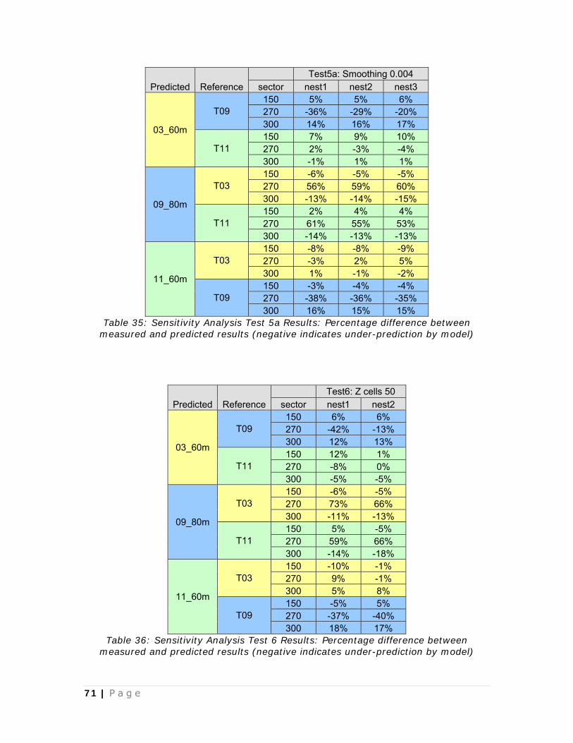
71 | P a g e

Predicted Reference Test5a: Smoothing 0.004 sector nest1 nest2 nest3

03_60m

T09 150 5% 5% 6% 270 -36% -29% -20% 300 14% 16% 17%

T11 150 7% 9% 10% 270 2% -3% -4% 300 -1% 1% 1%

09_80m

T03 150 -6% -5% -5% 270 56% 59% 60% 300 -13% -14% -15%

T11 150 2% 4% 4% 270 61% 55% 53% 300 -14% -13% -13%

11_60m

T03 150 -8% -8% -9% 270 -3% 2% 5% 300 1% -1% -2%

T09 150 -3% -4% -4% 270 -38% -36% -35% 300 16% 15% 15%

Table 35: Sensitivity Analysis Test 5a Results: Percentage difference between measured and predicted results (negative indicates under-prediction by model)

Predicted Reference Test6: Z cells 50 sector nest1 nest2

03_60m

T09 150 6% 6% 270 -42% -13% 300 12% 13%

T11 150 12% 1% 270 -8% 0% 300 -5% -5%

09_80m

T03 150 -6% -5% 270 73% 66% 300 -11% -13%

T11 150 5% -5% 270 59% 66% 300 -14% -18%

11_60m

T03 150 -10% -1% 270 9% -1% 300 5% 8%

T09 150 -5% 5% 270 -37% -40% 300 18% 17%

Table 36: Sensitivity Analysis Test 6 Results: Percentage difference between measured and predicted results (negative indicates under-prediction by model)

72 | P a g e

12.1.2 Turbulence Intensity 

Test Definition Test Nest Sector

Mast Absolute Average per nest

case

Absolute Average per test

case 03_60m 11_60m 09_80m 09_60m

Baseline Test1

nest1 150 3% 10% 0% -14% 7% 19% nest2 150 40% 22% 15% 1% 20%

nest3 150 49% 28% 28% 23% 32%

Segregated solver Test2

nest1 150 3% 20% 4% -11% 10% 30% nest2 150 51% 40% 30% 36% 39%

nest3 150 51% 48% 32% 39% 42%

Modified K-ε model Test3

nest1 150 0% 4% -10% -20% 8% 18% nest2 150 31% 10% 0% 3% 11%

nest3 150 50% 33% 25% 32% 35%

Forestry Test4 nest1 150 30% -440% 9% 13% 123%

104% nest2 150 32% -313% 5% 11% 90% nest3 150 44% -309% 18% 26% 99%

Smoothing 0.01 Test5

nest1 150 3% 10% 0% -14% 7% 19% nest2 150 37% 15% 14% 18% 21%

nest3 150 46% 24% 23% 29% 31%

Smoothing 0.004 Test5a

nest1 150 19% -5% -5% 0% 7% 8% nest2 150 0% 4% -6% -18% 7%

nest3 150 29% -3% -2% 6% 10% Z cells

50 Test6 nest1 150 -81% -128% -184% -137% 132% 73% nest2 150 7% -16% -22% -13% 14%

Table 37: Sensitivity Analysis TI Results for 150 sector: Percentage difference between measured and predicted results (negative indicates model over-prediction)

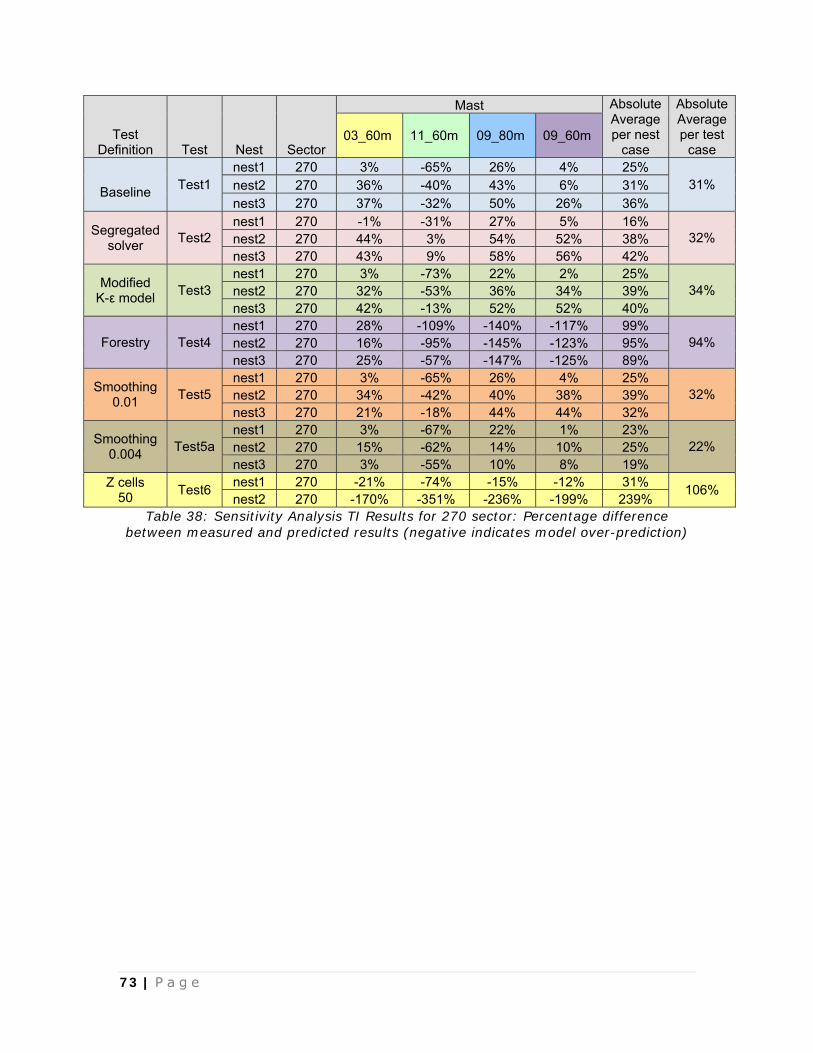
73 | P a g e

Test Definition Test Nest Sector

Mast Absolute Average per nest

case

Absolute Average per test

case 03_60m 11_60m 09_80m 09_60m

Baseline Test1

nest1 270 3% -65% 26% 4% 25% 31% nest2 270 36% -40% 43% 6% 31%

nest3 270 37% -32% 50% 26% 36%

Segregated solver Test2

nest1 270 -1% -31% 27% 5% 16% 32% nest2 270 44% 3% 54% 52% 38%

nest3 270 43% 9% 58% 56% 42%

Modified K-ε model Test3

nest1 270 3% -73% 22% 2% 25% 34% nest2 270 32% -53% 36% 34% 39%

nest3 270 42% -13% 52% 52% 40%

Forestry Test4 nest1 270 28% -109% -140% -117% 99%

94% nest2 270 16% -95% -145% -123% 95% nest3 270 25% -57% -147% -125% 89%

Smoothing 0.01 Test5

nest1 270 3% -65% 26% 4% 25% 32% nest2 270 34% -42% 40% 38% 39%

nest3 270 21% -18% 44% 44% 32%

Smoothing 0.004 Test5a

nest1 270 3% -67% 22% 1% 23% 22% nest2 270 15% -62% 14% 10% 25%

nest3 270 3% -55% 10% 8% 19% Z cells

50 Test6 nest1 270 -21% -74% -15% -12% 31% 106% nest2 270 -170% -351% -236% -199% 239%

Table 38: Sensitivity Analysis TI Results for 270 sector: Percentage difference between measured and predicted results (negative indicates model over-prediction)

74 | P a g e

Test Definition Test Nest Sector

Mast Absolute Average per nest

case

Absolute Average per test

case 03_60m 11_60m 09_80m 09_60m

Baseline Test1

nest1 300 -14% -101% -8% -37% 40% 36% nest2 300 16% -82% 5% -35% 34%

nest3 300 29% -38% 19% -53% 35%

Segregated solver Test2

nest1 300 -2% -49% 20% -19% 23% 33% nest2 300 45% -18% 44% 39% 37%

nest3 300 48% -12% 49% 46% 39%

Modified K-ε model Test3

nest1 300 -19% -107% -19% -45% 48% 36% nest2 300 4% -92% -11% -16% 31%

nest3 300 21% -80% 10% 11% 30%

Forestry Test4 nest1 300 -119% -136% -330% -301% 221%

206% nest2 300 -115% -130% -283% -260% 197% nest3 300 -112% -130% -288% -265% 199%

Smoothing 0.01 Test5

nest1 300 -14% -101% -8% -37% 40% 32% nest2 300 12% -83% 2% -2% 25%

nest3 300 24% -80% 11% 11% 31%

Smoothing 0.004 Test5a

nest1 300 -19% -102% -18% -46% 46% 36% nest2 300 33% -47% 24% 11% 29%

nest3 300 44% -44% 27% 20% 34% Z cells

50 Test6 nest1 300 -30% -86% -46% -47% 52% 118% nest2 300 -183% -334% -249% -229% 249%

Table 39: Sensitivity Analysis TI Results for 300 sector: Percentage difference between measured and predicted results (negative indicates model over-prediction)

75 | P a g e

12.2 Full Tests

12.2.1 Wind Speed Percentage Error per sector 

Sector  1 2 3 4 5 6 7 8 9 10 11 12 03_60m_to_09_45m   ‐2%  12%  ‐7%  ‐11%  ‐4%  ‐1%  ‐8%  ‐2%  28%  64%  ‐12%  ‐15% 03_60m_to_09_60m   ‐3%  17%  ‐4%  ‐13%  ‐4%  ‐2%  ‐8%  ‐3%  119%  62%  ‐11%  ‐17% 03_60m_to_09_80m   ‐4%  12%  1%  ‐16%  ‐4%  ‐5%  ‐9%  ‐5%  142%  58%  ‐12%  ‐20% 03_60m_to_11_45m   13%  ‐20%  ‐26%  ‐31%  ‐34%  ‐7%  32%  42%  110%  6%  7%  37% 03_60m_to_11_60m   10%  ‐21%  ‐29%  ‐31%  ‐34%  ‐7%  34%  39%  111%  6%  4%  34% 09_80m_to_03_60m   19%  ‐5%  4%  18%  10%  3%  43%  3%  10%  ‐21%  13%  57% 09_80m_to_11_60m   43%  ‐20%  ‐29%  ‐19%  ‐31%  ‐2%  45%  62%  4%  ‐33%  19%  69% 09_80m_to_11_45m   43%  ‐20%  ‐27%  ‐19%  ‐31%  ‐2%  44%  65%  1%  ‐33%  22%  73% 09_80m_to_09_60m   4%  5%  ‐3%  3%  1%  3%  2%  1%  5%  2%  1%  3% 09_80m_to_09_45m   9%  1%  ‐4%  5%  2%  4%  4%  1%  11%  3%  0%  6% 11_60m_to_03_60m   11%  29%  57%  43%  47%  5%  0%  ‐31%  51%  ‐6%  ‐5%  ‐7% 11_60m_to_09_45m   0%  38%  46%  28%  43%  6%  ‐28%  ‐32%  52%  54%  ‐16%  ‐38% 11_60m_to_09_60m   ‐3%  42%  48%  26%  43%  5%  ‐29%  ‐32%  44%  53%  ‐14%  ‐39% 11_60m_to_09_80m   ‐7%  36%  52%  23%  44%  2%  ‐30%  ‐33%  37%  49%  ‐16%  ‐41% 11_60m_to_11_45m   3%  ‐1%  6%  0%  ‐1%  0%  0%  2%  0%  0%  3%  3% 09_60m_to_03_60m   15%  ‐10%  7%  15%  9%  1%  39%  2%  6%  ‐22%  11%  53% 09_60m_to_11_45m   46%  ‐21%  ‐23%  ‐21%  ‐31%  ‐5%  41%  64%  1%  ‐35%  20%  68% 09_60m_to_11_60m   45%  ‐21%  ‐26%  ‐21%  ‐31%  ‐5%  41%  61%  4%  ‐35%  17%  63% 09_45m_to_11_60m   45%  ‐20%  ‐25%  ‐23%  ‐31%  ‐6%  39%  60%  5%  ‐35%  18%  59% 11_45m_to_09_80m   ‐10%  37%  44%  22%  45%  2%  ‐30%  ‐34%  37%  50%  ‐18%  ‐42% 

Table 40: Test A – 01 percentage error of WindSim predicted mean wind speed per sector for each cross prediction case.

Model errors are defined as 100 x (Upredicted – Umeasured)/Umeasured.

76 | P a g e

  Percentage Error per sector 

Sector  1 2 3 4 5 6 7 8 9 10 11 12 07_60m_to_07_45m   ‐12%  ‐64%  ‐53%  ‐13%  ‐10%  38%  97%  9%  ‐19%  ‐27%  10%  37% 07_60m_to_09_45m   ‐4%  ‐18%  ‐28%  31%  46%  42%  ‐4%  4%  ‐4%  ‐4%  ‐14%  0% 07_60m_to_09_60m   ‐9%  ‐15%  ‐27%  28%  46%  41%  ‐4%  2%  ‐10%  ‐4%  ‐13%  ‐3% 07_60m_to_09_80m   ‐13%  ‐16%  ‐25%  24%  55%  38%  ‐23%  ‐10%  ‐12%  13%  ‐15%  ‐13% 07_60m_to_10_45m   5%  ‐15%  ‐28%  64%  88%  74%  3%  ‐3%  ‐8%  ‐22%  ‐2%  17% 07_60m_to_10_60m   5%  ‐22%  ‐34%  67%  92%  62%  7%  7%  ‐47%  ‐24%  0%  19% 07_60m_to_11_45m   ‐9%  ‐63%  ‐54%  7%  9%  48%  72%  13%  ‐39%  ‐27%  14%  48% 07_60m_to_11_60m   ‐11%  ‐63%  ‐57%  8%  10%  49%  74%  14%  ‐39%  ‐27%  10%  45% 10_60m_to_10_45m   ‐1%  9%  10%  ‐2%  0%  7%  ‐4%  ‐10%  72%  3%  ‐1%  ‐1% 10_60m_to_07_45m   ‐6%  ‐47%  ‐33%  ‐46%  ‐53%  ‐17%  104% 42%  80%  ‐2%  7%  45% 10_60m_to_07_60m   ‐9%  ‐47%  ‐37%  ‐44%  ‐52%  ‐16%  105% 41%  74%  ‐2%  4%  41% 10_60m_to_09_45m   ‐4%  5%  10%  ‐15%  ‐24%  ‐13%  ‐3%  ‐2%  81%  32%  ‐11%  8% 10_60m_to_09_60m   ‐8%  12%  12%  ‐17%  ‐24%  ‐13%  2%  ‐5%  70%  32%  ‐10%  4% 10_60m_to_09_80m   ‐11%  17%  15%  ‐20%  ‐19%  ‐16%  ‐15%  ‐16%  65%  55%  ‐12%  ‐5% 10_60m_to_11_45m   ‐6%  ‐48%  ‐30%  ‐34%  ‐42%  ‐10%  89%  13%  15%  1%  17%  58% 10_60m_to_11_60m   ‐7%  ‐47%  ‐34%  ‐33%  ‐42%  ‐9%  94%  15%  15%  1%  12%  54% 07_45m_to_09_80m   ‐19%  ‐19%  ‐16%  32%  60%  38%  ‐31%  ‐12%  ‐13%  17%  ‐13%  ‐16% 10_45m_to_09_80m   ‐7%  12%  4%  ‐18%  ‐17%  ‐22%  ‐15%  ‐8%  ‐4%  51%  ‐12%  0% 07_45m_to_10_60m   ‐2%  ‐25%  ‐27%  77%  97%  63%  ‐4%  5%  ‐47%  ‐22%  1%  15% 07_45m_to_11_60m   ‐17%  ‐64%  ‐52%  14%  13%  50%  55%  12%  ‐39%  ‐24%  12%  40% 

Table 41: Test A – 02 percentage error of WindSim predicted mean wind speed per sector for each cross prediction case.

Model errors are defined as 100 x (Upredicted – Umeasured)/Umeasured.

77 | P a g e

Percentage Error per sector Sector  1 2 3 4 5 6 7 8 9 10 11 12

W59m_to_W40m   19%  12%  6% 5% 4% 8% 3% 3%  0%  ‐3% 0% 0%W59m_to_W50m   12%  4%  3% 3% 2% 4% 5% 3%  1%  1% 2% 1%W59m_to_U40m   0%  ‐4%  11% 13% 20% ‐6% 11% ‐6%  ‐4%  ‐6% 4% 9%W59m_to_U50m   ‐1%  ‐2%  13% 14% 13% ‐4% 14% ‐2%  0%  ‐7% 1% ‐2%W59m_to_U59m   ‐12%  ‐9%  7% 10% 8% ‐10% 3% ‐5%  ‐1%  ‐8% ‐2% ‐5%W59m_to_V41.5m   24%  3%  ‐4% ‐13% ‐17% ‐11% 13% ‐6%  1%  9% 0% 21%U59m_to_W40m   38%  21%  ‐2% ‐5% ‐4% 23% 12% 14%  ‐2%  6% 3% 0%U59m_to_W50m   31%  13%  ‐5% ‐7% ‐5% 18% 15% 14%  ‐1%  10% 4% 2%U59m_to_W59m   17%  9%  ‐8% ‐10% ‐8% 13% 11% 11%  ‐2%  9% 2% 0%U59m_to_U40m   13%  6%  4% 3% 11% 5% 8% ‐1%  ‐3%  3% 6% 15%U59m_to_U50m   12%  7%  6% 4% 4% 7% 11% 3%  1%  1% 3% 3%U59m_to_V41.5m   44%  9%  ‐12% ‐22% ‐24% ‐1% 14% 3%  1%  19% 2% 21%V41.5m_to_U40m   ‐18%  ‐6%  12% 28% 41% 4% ‐2% 1%  ‐4%  ‐12% 1% ‐12%V41.5m_to_U50m   ‐19%  ‐5%  15% 30% 33% 6% 0% 6%  ‐1%  ‐13% ‐2% ‐20%V41.5m_to_U59m   ‐27%  ‐11%  9% 25% 27% ‐1% ‐9% 3%  ‐1%  ‐14% ‐5% ‐23%V41.5m_to_W40m   ‐8%  1%  5% 16% 20% 15% 7% 9%  ‐4%  ‐9% ‐1% ‐19%V41.5m_to_W50m   ‐7%  2%  7% 17% 22% 17% 5% 11%  ‐2%  ‐7% 1% ‐17%V41.5m_to_W59m   ‐17%  ‐2%  4% 14% 19% 13% 1% 8%  ‐3%  ‐7% ‐1% ‐18%W50m_to_U50m   ‐12%  ‐7%  10% 11% 10% ‐7% 9% ‐4%  ‐2%  ‐8% 0% ‐4%W50m_to_U40m   ‐11%  ‐8%  7% 10% 17% ‐9% 7% ‐8%  ‐5%  ‐6% 2% 6%

Table 42: Test B – 01 percentage error of WindSim predicted mean wind speed per sector for each cross prediction case.

Model errors are defined as 100 x (Upredicted – Umeasured)/Umeasured.

78 | P a g e

Percentage Error per sector Sector  1 2 3 4 5 6 7 8 9 10 11 12

Y50m_to_Z40m   38%  24%  17%  ‐9%  ‐7%  10%  29%  21%  ‐2%  ‐8%  ‐4%  ‐18% Y50m_to_Z50m   38%  21%  16%  ‐13%  ‐9%  8%  24%  22%  ‐3%  ‐6%  ‐3%  ‐19% Y50m_to_X40m   19%  18%  ‐3%  ‐13%  ‐19%  ‐13%  19%  2%  ‐2%  2%  ‐5%  ‐19% Y50m_to_X50m   18%  15%  ‐5%  ‐16%  ‐19%  ‐14%  27%  14%  ‐3%  ‐2%  ‐6%  ‐19% Y50m_to_X59m   1%  6%  ‐9%  ‐19%  ‐23%  ‐20%  21%  13%  ‐4%  ‐4%  ‐10%  ‐22% Z50m_to_Y50m   ‐28%  ‐17%  ‐14%  13%  10%  ‐5%  ‐6%  ‐18%  1%  6%  4%  23% Z50m_to_Z40m   0%  2%  0%  4%  2%  2%  4%  ‐1%  0%  ‐2%  0%  0% Z50m_to_X40m   3%  ‐4%  ‐10%  ‐1%  ‐11%  ‐19%  4%  ‐10%  1%  9%  ‐2%  ‐2% Z50m_to_X50m   1%  ‐7%  ‐12%  ‐3%  ‐11%  ‐20%  11%  1%  ‐1%  5%  ‐3%  ‐2% Z50m_to_X59m   ‐15%  ‐14%  ‐16%  ‐7%  ‐16%  ‐25%  6%  ‐1%  ‐2%  2%  ‐6%  ‐5% X59m_to_Y50m   0%  ‐1%  7%  20%  34%  25%  ‐13%  ‐11%  2%  5%  12%  23% X59m_to_Z40m   37%  22%  26%  12%  21%  25%  14%  7%  0%  ‐4%  7%  1% X59m_to_Z50m   38%  19%  25%  7%  18%  24%  10%  7%  0%  ‐1%  7%  1% X59m_to_X40m   20%  13%  7%  7%  6%  9%  0%  ‐9%  3%  7%  5%  4% X59m_to_X50m   18%  9%  5%  4%  5%  7%  6%  2%  1%  2%  3%  4% X50m_to_Y50m   ‐15%  ‐9%  2%  14%  28%  18%  ‐17%  ‐12%  0%  2%  8%  18% X50m_to_Z40m   17%  12%  20%  7%  15%  17%  11%  5%  ‐1%  ‐6%  4%  ‐4% X50m_to_Z50m   18%  9%  19%  3%  13%  16%  6%  6%  ‐1%  ‐4%  4%  ‐4% X50m_to_X40m   2%  3%  2%  3%  1%  2%  ‐6%  ‐11%  2%  4%  1%  0% X50m_to_X59m   ‐15%  ‐8%  ‐5%  ‐4%  ‐4%  ‐6%  ‐5%  ‐1%  ‐1%  ‐2%  ‐3%  ‐4% 

Table 43: Test B – 02 percentage error of WindSim predicted mean wind speed per sector for each cross prediction case.

Model errors are defined as 100 x (Upredicted – Umeasured)/Umeasured.

79 | P a g e

Percentage Error per sector Sector  1 2 3 4 5 6 7 8 9 10 11 12

03_60m_to_09_45m   28%  25%  3%  ‐3%  ‐2%  ‐4%  14%  3%  268%  61%  ‐14%  3% 03_60m_to_09_60m   25%  36%  6%  ‐5%  ‐1%  ‐3%  12%  0%  245%  60%  ‐12%  1% 03_60m_to_09_80m   21%  30%  11%  ‐5%  0%  ‐5%  10%  ‐2%  222%  55%  ‐14%  0% 03_60m_to_11_45m   35%  ‐11%  ‐12%  ‐32%  ‐33%  ‐8%  52%  58%  141%  ‐5%  5%  76% 03_60m_to_11_60m   31%  ‐11%  ‐18%  ‐32%  ‐32%  ‐7%  52%  57%  138%  ‐5%  2%  70% 09_80m_to_03_60m   102%  12%  15%  21%  12%  0%  46%  21%  86%  ‐3%  14%  81% 09_80m_to_11_60m   91%  ‐15%  ‐15%  ‐25%  ‐29%  ‐3%  47%  84%  22%  ‐5%  18%  87% 09_80m_to_11_45m   102%  ‐15%  ‐8%  ‐26%  ‐29%  ‐4%  47%  84%  22%  ‐5%  21%  93% 09_80m_to_09_60m   81%  32%  9%  5%  4%  0%  9%  18%  77%  57%  1%  12% 09_80m_to_09_45m   88%  22%  7%  5%  3%  ‐1%  11%  20%  87%  58%  ‐1%  15% 11_60m_to_03_60m   21%  31%  48%  66%  51%  5%  20%  ‐21%  190%  1%  ‐1%  24% 11_60m_to_09_45m   13%  45%  37%  44%  40%  3%  ‐8%  ‐23%  192%  64%  ‐13%  ‐23% 11_60m_to_09_60m   9%  58%  39%  42%  43%  4%  ‐9%  ‐24%  173%  63%  ‐12%  ‐24% 11_60m_to_09_80m   7%  52%  47%  42%  46%  2%  ‐10%  ‐26%  155%  59%  ‐13%  ‐24% 11_60m_to_11_45m   19%  3%  18%  1%  ‐2%  0%  23%  20%  90%  ‐2%  5%  28% 09_60m_to_03_60m   102%  11%  18%  22%  12%  ‐2%  43%  19%  86%  ‐4%  12%  81% 09_60m_to_11_45m   102%  ‐15%  ‐5%  ‐25%  ‐29%  ‐6%  44%  82%  22%  ‐6%  18%  93% 09_60m_to_11_60m   91%  ‐16%  ‐13%  ‐25%  ‐28%  ‐5%  44%  81%  22%  ‐5%  15%  87% 09_45m_to_11_60m   90%  ‐13%  ‐12%  ‐25%  ‐28%  ‐5%  44%  79%  23%  ‐3%  16%  87% 11_45m_to_09_80m   3%  49%  40%  41%  46%  2%  ‐9%  ‐24%  160%  59%  ‐15%  ‐26% 

Table 44: Test A – 01 percentage error of WAsP predicted mean wind speed per sector for each cross prediction case.

Model errors are defined as 100 x (Upredicted – Umeasured)/Umeasured.

80 | P a g e

Percentage Error per sector Sector  1 2 3 4 5 6 7 8 9 10 11 12

07_60m_to_07_45m   27%  12%  39%  ‐3%  2%  1%  54%  26%  67%  ‐2%  ‐3%  11% 07_60m_to_09_45m   5%  ‐19%  ‐12%  25%  37%  40%  40%  9%  67%  ‐2%  ‐14%  2% 07_60m_to_09_60m   1%  ‐14%  ‐8%  23%  37%  38%  36%  9%  53%  ‐2%  ‐12%  0% 07_60m_to_09_80m   ‐1%  ‐16%  ‐3%  20%  44%  33%  9%  ‐2%  52%  18%  ‐13%  ‐7% 07_60m_to_10_45m   27%  ‐19%  ‐11%  62%  82%  70%  48%  ‐3%  50%  ‐25%  3%  37% 07_60m_to_10_60m   27%  ‐24%  ‐17%  67%  81%  55%  53%  5%  ‐11%  ‐27%  3%  37% 07_60m_to_11_45m   0%  ‐68%  ‐33%  ‐5%  2%  53%  154%  29%  ‐8%  ‐29%  12%  61% 07_60m_to_11_60m   ‐3%  ‐68%  ‐38%  ‐3%  2%  52%  155%  34%  ‐8%  ‐29%  9%  57% 10_60m_to_10_45m   27%  36%  5%  ‐1%  9%  7%  31%  28%  213%  3%  0%  54% 10_60m_to_07_45m   26%  87%  54%  ‐41%  ‐40%  ‐38%  34%  68%  238%  31%  ‐6%  24% 10_60m_to_07_60m   19%  79%  63%  ‐39%  ‐39%  ‐38%  16%  65%  233%  36%  ‐4%  20% 10_60m_to_09_45m   8%  33%  ‐3%  ‐24%  ‐18%  ‐12%  26%  45%  246%  33%  ‐14%  16% 10_60m_to_09_60m   3%  43%  1%  ‐25%  ‐18%  ‐12%  24%  43%  215%  32%  ‐12%  13% 10_60m_to_09_80m   1%  42%  7%  ‐27%  ‐13%  ‐14%  0%  29%  205%  57%  ‐14%  3% 10_60m_to_11_45m   3%  ‐47%  ‐30%  ‐42%  ‐39%  ‐5%  124%  70%  87%  ‐5%  11%  81% 10_60m_to_11_60m   0%  ‐47%  ‐35%  ‐41%  ‐39%  ‐4%  129%  75%  87%  ‐5%  7%  76% 07_45m_to_09_80m   ‐7%  ‐19%  1%  24%  45%  30%  1%  ‐7%  57%  22%  ‐11%  ‐9% 10_45m_to_09_80m   5%  33%  1%  ‐26%  ‐16%  ‐20%  ‐5%  8%  209%  53%  ‐15%  9% 07_45m_to_10_60m   20%  ‐28%  ‐14%  72%  81%  52%  40%  2%  ‐7%  ‐23%  5%  36% 07_45m_to_11_60m   ‐9%  ‐69%  ‐35%  0%  2%  49%  137%  27%  ‐5%  ‐26%  11%  55% 

Table 45: Test A – 02 percentage error of WAsP predicted mean wind speed per sector for each cross prediction case.

Model errors are defined as 100 x (Upredicted – Umeasured)/Umeasured.

81 | P a g e

Percentage Error per sector Sector  1 2 3 4 5 6 7 8 9 10 11 12

W59m_to_W40m   24%  13%  4%  3%  5%  18%  5%  9%  ‐4%  ‐4%  ‐1%  ‐5% W59m_to_W50m   4%  ‐4%  ‐17%  ‐11%  5%  6%  12%  ‐2%  ‐9%  ‐7%  5%  0% W59m_to_U40m   6%  ‐1%  13%  21%  15%  ‐11%  ‐5%  ‐4%  ‐1%  ‐5%  7%  6% W59m_to_U50m   3%  ‐3%  13%  23%  10%  ‐8%  ‐1%  ‐2%  1%  ‐6%  3%  ‐5% W59m_to_U59m   ‐7%  ‐9%  7%  18%  6%  ‐12%  ‐7%  ‐4%  1%  ‐6%  1%  ‐7% W59m_to_V41.5m   36%  0%  ‐4%  ‐7%  ‐13%  ‐6%  ‐3%  ‐4%  ‐4%  5%  ‐1%  15% U59m_to_W40m   39%  24%  ‐3%  ‐12%  ‐3%  30%  22%  19%  ‐6%  1%  ‐2%  ‐2% U59m_to_W50m   16%  6%  ‐22%  ‐24%  ‐3%  17%  30%  7%  ‐10%  ‐2%  4%  4% U59m_to_W59m   19%  13%  ‐8%  ‐15%  ‐4%  23%  27%  19%  ‐5%  4%  ‐1%  ‐1% U59m_to_U40m   19%  11%  7%  4%  9%  3%  5%  6%  ‐2%  ‐1%  6%  11% U59m_to_U50m   15%  9%  7%  5%  3%  6%  11%  9%  0%  ‐2%  2%  1% U59m_to_V41.5m   54%  10%  ‐11%  ‐21%  ‐18%  3%  9%  6%  ‐5%  11%  ‐2%  21% V41.5m_to_U40m   ‐19%  ‐1%  15%  29%  32%  3%  6%  4%  ‐2%  ‐9%  5%  ‐11% V41.5m_to_U50m   ‐22%  ‐3%  17%  31%  25%  5%  9%  8%  1%  ‐10%  0%  ‐19% V41.5m_to_U59m   ‐29%  ‐10%  11%  25%  21%  1%  4%  4%  0%  ‐10%  ‐2%  ‐20% V41.5m_to_W40m   ‐2%  14%  8%  11%  18%  35%  17%  17%  ‐5%  ‐9%  ‐4%  ‐19% V41.5m_to_W50m   ‐19%  ‐3%  ‐14%  ‐5%  19%  21%  25%  5%  ‐10%  ‐11%  2%  ‐13% V41.5m_to_W59m   ‐17%  3%  2%  6%  17%  26%  23%  17%  ‐4%  ‐5%  ‐3%  ‐18% W50m_to_U50m   ‐7%  ‐8%  9%  21%  6%  ‐10%  ‐1%  ‐4%  1%  ‐6%  2%  ‐7% W50m_to_U40m   ‐4%  ‐6%  9%  19%  12%  ‐12%  ‐7%  ‐5%  ‐2%  ‐5%  6%  2% 

Table 46: Test B – 01 percentage error of WAsP predicted mean wind speed per sector for each cross prediction case.

Model errors are defined as 100 x (Upredicted – Umeasured)/Umeasured.

82 | P a g e

Percentage Error per sector Sector  1 2 3 4 5 6 7 8 9 10 11 12

Y50m_to_Z40m   38%  45%  16%  ‐2%  0%  16%  19%  21%  ‐7%  ‐10%  ‐4%  ‐19% Y50m_to_Z50m   44%  40%  17%  ‐6%  ‐2%  14%  16%  22%  ‐7%  ‐8%  ‐2%  ‐19% Y50m_to_X40m   27%  34%  ‐5%  ‐19%  ‐21%  ‐9%  3%  5%  ‐3%  ‐6%  ‐10%  ‐21% Y50m_to_X50m   27%  29%  ‐6%  ‐22%  ‐19%  ‐10%  8%  21%  ‐4%  ‐8%  ‐10%  ‐20% Y50m_to_X59m   8%  20%  ‐9%  ‐24%  ‐23%  ‐14%  5%  23%  ‐4%  ‐10%  ‐12%  ‐21% Z50m_to_Y50m   ‐21%  ‐28%  ‐13%  4%  17%  2%  10%  ‐6%  4%  5%  2%  14% Z50m_to_Z40m   7%  4%  ‐1%  2%  5%  12%  14%  8%  ‐2%  ‐5%  ‐1%  ‐3% Z50m_to_X40m   12%  1%  ‐15%  ‐16%  ‐16%  ‐11%  ‐1%  ‐2%  3%  0%  ‐7%  ‐8% Z50m_to_X50m   10%  ‐4%  ‐15%  ‐18%  ‐14%  ‐12%  6%  12%  0%  ‐3%  ‐8%  ‐6% Z50m_to_X59m   ‐7%  ‐11%  ‐18%  ‐21%  ‐19%  ‐15%  2%  13%  0%  ‐4%  ‐9%  ‐7% X59m_to_Y50m   ‐4%  ‐16%  5%  28%  49%  28%  12%  ‐10%  ‐1%  9%  12%  16% X59m_to_Z40m   29%  21%  20%  27%  34%  43%  18%  5%  ‐7%  ‐2%  9%  ‐2% X59m_to_Z50m   35%  18%  21%  20%  31%  40%  14%  6%  ‐6%  0%  10%  ‐2% X59m_to_X40m   28%  18%  4%  4%  7%  14%  8%  ‐6%  ‐1%  5%  2%  ‐6% X59m_to_X50m   27%  13%  3%  1%  8%  12%  14%  8%  ‐4%  2%  1%  ‐4% X50m_to_Y50m   ‐16%  ‐24%  ‐1%  23%  43%  23%  11%  ‐10%  ‐2%  7%  10%  10% X50m_to_Z40m   13%  12%  14%  22%  28%  35%  16%  5%  ‐7%  ‐3%  7%  ‐6% X50m_to_Z50m   17%  8%  16%  16%  25%  32%  13%  6%  ‐7%  ‐1%  8%  ‐7% X50m_to_X40m   14%  10%  ‐1%  0%  2%  9%  4%  ‐6%  ‐2%  3%  1%  ‐9% X50m_to_X59m   ‐3%  ‐3%  ‐6%  ‐5%  ‐2%  2%  7%  8%  ‐4%  ‐1%  ‐2%  ‐8% 

Table 47: Test B – 02 percentage error of WAsP predicted mean wind speed per sector for each cross prediction case.

Model errors are defined as 100 x (Upredicted – Umeasured)/Umeasured.

83 | P a g e

 

12.2.2 TI 

Individual Model Prediction Error (TI Corrected) 1  2  3  4  5  6  7  8  9  10  11  12 

11_60m IWeng  75%  64%  ‐11%  65%  32%  ‐2%  ‐  ‐  12%  30%  42%  46% IWSim  54%  52%  ‐8%  24%  28%  ‐1%  ‐  ‐  13%  45%  58%  40% 

11_45m IWeng  ‐  56%  ‐4%  51%  20%  ‐5%  ‐  ‐  3%  23%  22%  22% IWSim  ‐  62%  4%  29%  25%  2%  ‐  ‐  20%  46%  45%  28% 

03_60m IWeng  ‐  ‐  ‐  ‐  ‐1%  ‐11% ‐  ‐  ‐  ‐5%  ‐3%  16% IWSim  ‐  ‐  ‐  ‐  3%  ‐19% ‐  ‐  ‐  ‐1%  3%  24% 

09_80m IWeng  ‐  ‐  ‐  ‐21%  96%  34%  ‐1%  89%  ‐  11%  36%  63% IWSim  ‐  ‐  ‐  ‐32%  66%  9%  ‐36%  17%  ‐  3%  27%  73% 

09_60m IWeng  ‐  ‐  ‐  ‐8%  81%  5%  ‐12%  ‐  ‐  5%  26%  39% IWSim  ‐  ‐  ‐  ‐19%  73%  ‐2%  ‐32%  ‐  ‐  1%  28%  49% 

09_45m IWeng  ‐  ‐  ‐  ‐  72%  11%  ‐  ‐  ‐  6%  25%  23% IWSim  ‐  ‐  ‐  ‐  67%  6%  ‐  ‐  ‐  7%  35%  36% 

07_60m IWeng  ‐  ‐  ‐  6%  57%  30%  ‐20%  ‐  ‐  ‐22%  ‐16%  68% IWSim  ‐  ‐  ‐  5%  54%  24%  ‐27%  ‐  ‐  ‐18%  ‐12%  72% 

07_45m IWeng  ‐  ‐  ‐  ‐7%  36%  16%  ‐28%  ‐  ‐  ‐20%  ‐19%  53% IWSim  ‐  ‐  ‐  6%  55%  29%  ‐22%  ‐  ‐  ‐11%  ‐10%  64% 

10_60m IWeng  ‐  ‐  ‐  ‐  ‐  ‐14% ‐  ‐  ‐  ‐15%  ‐13%  ‐ IWSim  ‐  ‐  ‐  ‐  ‐  ‐20% ‐  ‐  ‐  ‐44%  ‐7%  ‐ 

10_45m IWeng  ‐  ‐  ‐  ‐  ‐22%  ‐16% ‐  ‐  ‐  ‐18%  ‐29%  ‐ IWSim  ‐  ‐  ‐  ‐  ‐11%  ‐17% ‐  ‐  ‐  ‐35%  ‐18%  ‐ 

Table 48: Individual mast and sector TI prediction results from both models for Site A. TI has been corrected according to Equation 18 (Negative indicates model under

prediction).

84 | P a g e

Individual Model Prediction Error (TI Corrected) 

1  2  3  4  5  6  7  8  9  10  11  12 

11_60m IWeng  133%  118%  18%  120% 77%  31%  ‐  ‐  49%  73%  90%  95% IWSim  105%  103%  22%  66%  70%  32%  ‐  ‐  51%  94%  110%  86% 

11_45m IWeng  ‐  108%  29%  102% 60%  27%  ‐  ‐  37%  64%  62%  62% IWSim  ‐  116%  39%  72%  66%  36%  ‐  ‐  61%  94%  93%  71% 

03_60m IWeng  ‐  ‐  ‐  ‐  32%  19%  ‐  ‐  ‐  26%  29%  55% IWSim  ‐  ‐  ‐  ‐  37%  9%  ‐  ‐  ‐  32%  38%  66% 

09_80m IWeng  ‐  ‐  ‐  5%  161%  78%  32%  152%  ‐  48%  81%  118% IWSim  ‐  ‐  ‐  ‐9%  121%  46%  ‐15%  56%  ‐  38%  69%  130% 

09_60m IWeng  ‐  ‐  ‐  22%  141%  40%  17%  ‐  ‐  40%  68%  86% IWSim  ‐  ‐  ‐  8%  131%  30%  ‐9%  ‐  ‐  34%  70%  99% 

09_45m IWeng  ‐  ‐  ‐  ‐  130%  49%  ‐  ‐  ‐  42%  67%  64% IWSim  ‐  ‐  ‐  ‐  122%  41%  ‐  ‐  ‐  43%  80%  81% 

07_60m IWeng  ‐  ‐  ‐  41%  109%  74%  7%  ‐  ‐  4%  11%  124% IWSim  ‐  ‐  ‐  40%  105%  66%  ‐3%  ‐  ‐  9%  17%  130% 

07_45m IWeng  ‐  ‐  ‐  24%  81%  55%  ‐4%  ‐  ‐  7%  8%  104% IWSim  ‐  ‐  ‐  41%  107%  73%  4%  ‐  ‐  19%  20%  118% 

10_60m IWeng  ‐  ‐  ‐  ‐  ‐  14%  ‐  ‐  ‐  13%  16%  ‐ IWSim  ‐  ‐  ‐  ‐  ‐  6%  ‐  ‐  ‐  ‐26%  24%  ‐ 

10_45m IWeng  ‐  ‐  ‐  ‐  4%  12%  ‐  ‐  ‐  10%  ‐5%  ‐ IWSim  ‐  ‐  ‐  ‐  19%  11%  ‐  ‐  ‐  ‐14%  9%  ‐ 

Table 49: Individual mast and sector TI prediction results from both models for Site A. No TI correction has been applied. (Negative indicates model under prediction).

85 | P a g e

Individual Model Prediction Error (TI Corrected) 1  2  3  4  5  6  7  8  9  10  11  12 

V42 IWeng  ‐  ‐24%  ‐24%  3%  ‐15%  ‐  ‐  ‐11%  ‐8%  ‐21%  ‐17%  ‐30% IWSim  ‐  ‐21%  ‐9%  8%  ‐8%  ‐  ‐  ‐30%  ‐29%  ‐53%  ‐46%  ‐25% 

U59 IWeng  ‐27%  ‐11%  1%  ‐16%  ‐8%  ‐  ‐  ‐6%  ‐1%  ‐15%  ‐21%  ‐27% IWSim  ‐21%  6%  0%  ‐13%  ‐10%  ‐  ‐  ‐33%  ‐44%  ‐48%  ‐46%  ‐28% 

U50 IWeng  ‐  ‐  ‐12%  ‐18%  ‐12%  ‐  ‐  ‐  ‐6%  ‐16%  ‐19%  ‐26% IWSim  ‐  ‐  ‐8%  ‐9%  ‐6%  ‐  ‐  ‐  ‐37%  ‐43%  ‐38%  ‐22% 

U40 IWeng  ‐  4%  ‐25%  ‐27%  ‐26%  ‐  ‐  ‐  ‐16%  ‐24%  ‐35%  ‐32% IWSim  ‐  37%  ‐16%  ‐13%  ‐13%  ‐  ‐  ‐  ‐32%  ‐41%  ‐43%  ‐22% 

W59 IWeng  ‐15%  ‐9%  1%  3%  0%  ‐  ‐  ‐47%  ‐34%  ‐50%  ‐13%  ‐19% IWSim  ‐7%  ‐3%  ‐6%  ‐8%  3%  ‐  ‐  ‐60%  ‐35%  ‐59%  ‐44%  ‐40% 

W50 IWeng  ‐  ‐16%  ‐6%  5%  1%  ‐  ‐  ‐36%  ‐18%  ‐33%  3%  ‐19% IWSim  ‐  ‐8%  ‐10%  ‐2%  7%  ‐  ‐  ‐58%  ‐36%  ‐53%  ‐35%  ‐31% 

W40 IWeng  ‐  ‐25%  ‐15%  2%  ‐1%  ‐  ‐  ‐25%  ‐6%  ‐8%  4%  ‐24% IWSim  ‐  ‐13%  ‐13%  0%  9%  ‐  ‐  ‐52%  ‐37%  ‐42%  ‐30%  ‐24% 

Y50 IWeng  ‐  ‐  25%  ‐7%  ‐  ‐  ‐52%  ‐43%  ‐63%  ‐69%  ‐57%  ‐51% IWSim  ‐  ‐  15%  ‐17%  ‐  ‐  ‐32%  2%  0%  2%  ‐15%  ‐41% 

Z50 IWeng  ‐  ‐  1%  0%  ‐  ‐  ‐  13%  26%  23%  5%  ‐7% IWSim  ‐  ‐  ‐6%  ‐5%  ‐  ‐  ‐  ‐17%  ‐12%  ‐15%  ‐15%  ‐6% 

Z40 IWeng  ‐  ‐  3%  ‐2%  ‐  ‐  ‐  7%  22%  19%  0%  ‐14% IWSim  ‐  ‐  1%  ‐1%  ‐  ‐  ‐  ‐12%  ‐10%  ‐13%  ‐13%  ‐7% 

X59 IWeng  ‐  9%  29%  46%  27%  ‐  ‐  12%  8%  4%  10%  ‐9% IWSim  ‐  13%  15%  16%  12%  ‐  ‐  ‐11%  ‐17%  ‐29%  ‐23%  ‐23% 

X50 IWeng  ‐  ‐  19%  29%  19%  ‐  ‐  12%  21%  8%  15%  ‐9% IWSim  ‐  ‐  10%  7%  9%  ‐  ‐  ‐6%  ‐5%  ‐25%  ‐16%  ‐19% 

X40 IWeng  ‐  ‐  5%  18%  11%  ‐  ‐  7%  11%  0%  10%  ‐13% IWSim  ‐  ‐  3%  3%  6%  ‐  ‐  ‐1%  ‐7%  ‐27%  ‐14%  ‐15% 

Table 50: Individual mast and sector TI prediction results from both models for Site B. TI has been corrected according to Equation 18 (Negative indicates model under

prediction).

86 | P a g e

Individual Model Prediction Error (TI Corrected)

1 2 3 4 5 6 7 8 9 10 11 12

V42 IWeng - 2% 1% 37% 13% - - 19% 23% 5% 10% -6% IWSim - 6% 21% 44% 23% - - -7% -5% -37% -28% 0%

U59 IWeng -3% 18% 35% 12% 22% - - 26% 32% 14% 5% -3% IWSim 5% 42% 34% 16% 20% - - -11% -25% -30% -29% -4%

U50 IWeng - - 17% 9% 17% - - - 25% 12% 8% -2% IWSim - - 23% 22% 26% - - - -16% -24% -18% 4%

U40 IWeng - 38% 0% -3% -1% - - - 12% 1% -13% -9% IWSim - 83% 11% 16% 16% - - - -9% -21% -25% 4%

W59 IWeng 14% 21% 34% 38% 33% - - -29% -12% -34% 16% 7% IWSim 24% 29% 25% 23% 37% - - -47% -13% -45% -25% -20%

W50 IWeng - 12% 25% 40% 35% - - -15% 9% -11% 37% 8% IWSim - 23% 21% 31% 42% - - -44% -15% -38% -14% -8%

W40 IWeng - 0% 13% 36% 32% - - 0% 25% 22% 39% 2% IWSim - 16% 16% 33% 45% - - -36% -16% -23% -7% 1%

Y50 IWeng - - 67% 24% - - -37% -24% -51% -58% -43% -35% IWSim - - 53% 10% - - -9% 37% 34% 35% 14% -21%

Z50 IWeng - - 34% 33% - - - 51% 68% 64% 40% 24% IWSim - - 25% 27% - - - 11% 17% 14% 13% 26%

Z40 IWeng - - 38% 31% - - - 42% 63% 58% 33% 15% IWSim - - 34% 32% - - - 17% 20% 16% 17% 25%

X59 IWeng - 45% 71% 95% 69% - - 50% 44% 39% 47% 22% IWSim - 50% 53% 55% 49% - - 18% 10% -5% 3% 3%

X50 IWeng - - 58% 72% 59% - - 49% 61% 44% 53% 21% IWSim - - 47% 42% 46% - - 25% 27% 0% 12% 9%

X40 IWeng - - 40% 58% 47% - - 42% 47% 33% 47% 16% IWSim - - 38% 37% 42% - - 32% 25% -3% 15% 13%

Table 51: Individual mast and sector TI prediction results from both models for Site B. No TI correction has been applied. (Negative indicates model under prediction).

87 | P a g e

12.3 Navier-Stokes Equations The Navier-Stokes equations are based on the assumption that the fluid is a continuous substance (and not a discrete collection of particles). The derivation of the Navier-Stokes equations is a complex process and the below is very much a summary version of this, with much detail omitted. The interested reader should refer to the Wikipedia and CFD Online websites (1) (30) for a complete and readily available source. The derivation of the Navier-Stokes equations begins with the conservation of mass, momentum and (optionally) energy being written for a control volume (a finite arbitrary volume).

· 0 Equation 19

Making use of the continuity equation, which states that the changes of some state variable (L) defined over a control volume must be equal to what is lost (or gained) through the boundaries of the volume plus what is created or consumed by sources and sinks inside the control volume. Where Q represents source and sink terms in the fluid, t is time and U the velocity of the fluid. Based on this principle, the concepts of conservation of mass, conservation of momentum and conservation of energy may be written.

12.3.1 Conservation of Momentum  Using the above continuity equation and applying this to momentum (ρνi, where ρ is density and v the velocity) yields:

· 0 Equation 20

With the subscript “i” indicating that the above equation is applied to each component of velocity, u, (generally u, v and w). Noting that a body force, b, is a source or sink of momentum (which effectively replaces the Q term) and expanding the derivatives completely yields

· · · Equation 21

Making use of the relationship

· · · Equation 22

88 | P a g e

And through further rearrangement we arrive at

·  Equation 23

12.3.2 Conservation of Mass  Mass may also be considered, though there are no sources or sinks of mass, so Q=0. Putting density into the continuity equation gives

· 0 Equation 24

In the case of an incompressible fluid, density is a constant and the equation reduces to:

· 0 Equation 25

12.3.3 Incompressible Flow  From Equation 23, the generic body force term (b) is broken up into two new terms, one describing forces resulting from stresses and one for “other” forces such as gravity or centrifugal forces. WindSim is based on a form of the Navier-Stokes equations for an incompressible fluid, a generic form of which is given below in vector form below. This form appears quite different to that given in section 3.1.4, however the incompressible flow equation is given here in this notation to provide the reader with a better understanding as to the different components of the equation:

· Equation 26

Where f represents the “other” body forces, P represents pressure, is the viscosity and the viscosity term arises from the viscous shear forces. The only non-linear term in this equation is the convective term.

Inertia

Other Forces

Viscosity Pressure Gradient

Convective Acceleration

Unsteady Acceleration

89 | P a g e

Expressing this equation in Cartesian coordinates is given below

Equation 27 Where u, v, and w as given in the above equation are the three directional components of velocity and the final gravity terms in the first two lines will be zero if conventional coordinates (x, y, z) are chosen. And the continuity equation becomes

0 Equation 28