02072010 SoilCAM deliverable D1 2 - Nibio - Nibio1/SoilCAM_deliverable_D1.2.pdf · 2.3.3 Uncertainties in electrical resistivity interpretation ... processing, non-uniqueness of the

Optimisation of geophysical field methods

Deliverable D 1.2

Alberto Godio

Merhdad Bastani

Helen French

Esther Bloem

Sebastiano Foti

Alessandro Arato

Stefano Stocco

Laust Pedersen

3 Deliverable 1.2

Soil Contamination: Advanced integrated characterisation and time-lapse Monitoring

Title Optimisitaion of geophysical field methods

Authors Alberto Godio, Merhdad Bastani,Helen French

Esther Bloem, Sebastiano Foti, Alessandro Arato

Laust Pedersen

Deliverable No. Deliverable D 1.2

ISBN

Organisation name of lead

contractor for this deliverable

POLITO

No. of pages 86

Due date of deliverable: November, 2009 (18 month) – changed to June, 2010

Dissemination level RE

Key words geophysical methods, experimental design

Title of project: Soil Contamination: Advanced integrated characterisation and time

lapse Monitoring (SoilCAM)

Instrument: 6.3 Environmental technologies, Topic ENV.2007.3.1.2.2, Development of

technologies and tools for soil contamination assessment and site

Contract number: 212663

Start date of project: June 2008, Duration: 48 months

Project co-funded by the European Commission within the Seventh Framework Programme (2008-2012)

Disclaimer

The information provided and the opinions given in this publication are not necessarily those of the consortium or

the EC. The authors and publisher assume no liability for any loss resulting from the use of this report.

4 Deliverable 1.2

Summary

The deliverable 1.2 (month 18) summarizes the preliminary results for the enhancement of the geophysical

field methods according to the following challenges:

how the forward modeling and sensitivity analysis of electrical and electromagnetic methods can be

useful to optimise the geophysical procedures;

how the existing a priori data (geological, geochemical…) can be incorporated in the geophysical

data set;

the integration of geophysical methods for soil mapping with the innovative strategies for detailed

monitoring of hot-spots using both electromagnetic methods and surface/cross borehole georadar

and electrical time lapse survey;

how the integrated geophysical methods are effective to estimate the site specific constitutive

relationships between the geophysical signature and the petrophysical parameters at Trecate and

Gardermoen sites;

how the periodic seasonal grid-like surface measurements and borehole surveys are effective to

estimate the changes the soil properties variations.

The previous tasks are discussed by theoretical evaluating and analysis of the available data set of

geophysical and soil sampling at the two test sites.

We concentrate the work on the analysis of experimental design and sensitivity analysis as a tool to optimise

the survey, according to the equipment capability, the expected target response, the experimental

uncertainties and the background noise.

The main description of the experimental part of the work is focused on the analysis of time-lapse monitoring

of the variation of electrical and electromagnetic parameters and their relation with temporal and spatial

changes of moisture content. We briefly discuss the uncertainties and accuracy and strategies to incorporate

a priori information on the interpretation process.

5 Deliverable 1.2

Content

1. INTRODUCTION ............................................................................................................. 7

2. SURVEY DESIGN .......................................................................................................... 10

2.1 The geophysical model of the sites ............................................................................................... 11 2.1.1 Trecate site ............................................................................................................................... 12 2.1.2 The Gardermoen site ................................................................................................................ 17

2.2 The experimental design ............................................................................................................... 20 2.2.1 The model framework .............................................................................................................. 21 2.2.2 Forward modeling of Slingram survey ..................................................................................... 22 2.2.3 The 1D electromagnetic modeling of Trecate site .................................................................... 22 2.2.4 The statistical experimental design .......................................................................................... 26 2.2.5 Survey design of electrical resistivity tomography (ERT) ....................................................... 29

2.3 Time-lapse survey .......................................................................................................................... 33 2.3.1 Time lapse surveys for cross borehole georadar ...................................................................... 33 2.3.2 Time lapse electrical resistivity ................................................................................................ 35 2.3.3 Uncertainties in electrical resistivity interpretation .................................................................. 35

3. TIME LAPSE SURVEYS AT TRECATE SITE ......................................................... 37

3.1 Set up of the test site ...................................................................................................................... 38 3.1.1 Borehole electrical resistivity ................................................................................................... 39 3.1.2 Noise sources ............................................................................................................................ 40 3.1.3 Constrains ................................................................................................................................. 42 3.1.4 Results ...................................................................................................................................... 42

3.2 Georadar time lapse data .............................................................................................................. 46 3.2.1 ZOP data acquisition ................................................................................................................ 46 3.2.2 Analysis of time lapse data of April, 2008 ............................................................................... 47 3.2.3 Attribute analysis of GPR signature ......................................................................................... 49

4. TIME-LAPSE SURVEYS AT GARDERMOEN ......................................................... 53

4.1 Time-lapse GPR survey at Oslo airport ...................................................................................... 53 4.1.1 GPR data processing ................................................................................................................ 56 4.1.2 Results ...................................................................................................................................... 57 4.1.3 Time-lapse survey .................................................................................................................... 59

4.2 Time-lapse DC-resistivity measurements at Oslo airport .......................................................... 60 4.2.1 Inverse modelling results .......................................................................................................... 61 4.2.2 Hydra Probes data, Oslo airport ............................................................................................... 64 4.2.3 Slingram measurement at Oslo airport ..................................................................................... 67

4.3 Experiments at Moreppen site ..................................................................................................... 67 4.3.1 Data acquisition ........................................................................................................................ 68 4.3.2 Data analysis............................................................................................................................. 68

6 Deliverable 1.2

4.3.3 Inversion ................................................................................................................................... 73 4.3.4 Results ...................................................................................................................................... 73

5. RECOMMENDATIONS ................................................................................................ 76

5.1 Soil heterogeneity .......................................................................................................................... 76

5.2 Experimental design ...................................................................................................................... 77

5.3 Data inversion ................................................................................................................................ 77

5.4 Time lapse data .............................................................................................................................. 78

5.5 Hydraulic properties and contaminants ...................................................................................... 79

6. REFERENCES ................................................................................................................ 81

7. APPENDIX ...................................................................................................................... 86

7 Deliverable 1.2

1. Introduction

The effectiveness of geophysical methods for monitoring the contaminated site is mainly

conditioned by the experimental design, accuracy, uncertainties, the bias introduced by the data

processing, non-uniqueness of the geophysical solution and ambiguities in the translating the

geophysical data into a realistic geological or hydrogeological model.

The optimisation of the geophysical technique in the context of the SoilCAm project is focused:

to optimise the sensitivity of the adopted methods to the spatial and temporal variations of the

geophysical parameters according to the expected changes of the soil properties; the soil

properties can be related to the lithological heterogeneity, local hydrological conditions and the

bio-geochemical activity;

To enhance the procedure of the time lapse survey in order to reduce the uncertainties

propagation in the inversion process and to include a priori information.

These tasks can be obtained by considering the following procedure:

estimate the main petrophysical relationships for the two test sites;

design the optimal configuration of the geophysical experiments for an optimal sensitivity

according to the soil stratigraphy and to the expected changes of soil properties;

define the best strategies for minimising the uncertainties propagation during the inversion

process; at this stage of the project this issue is analysed for the cross-borehole investigation

of the borehole georadar survey only

The project is focused on the assessment of geophysical methods for the improving in the

knowledge of the hydrogeological setting of the test sites and monitoring the clean up of the

contamination; in such a context, we’re developing new strategies:

to evaluate the reliability of time-lapse geophysics in the assessment of the temporal

changes of the hydrological conditions (water content distribution);

to analysis the effectiveness of the integrated geophysical approaches for monitoring

sustainable remediation (monitoring natural attenuation - MNA) of the subsoil.

The main challenges in the optimisation of the electrical and electromagnetic methods, applied at the

two test sites, require:

to define the best strategies for the experimental design of surface electrical and

electromagnetic measurements with respect to resolution, sensitivity and uncertainties;

the optimisation of data acquisition of the borehole electrical resistivity and cross-hole

georadar monitoring in time lapse monitoring with respect to sensitivity, uncertainties

the analysis of the solution of ill-posed problem in cross hole tomography;

8 Deliverable 1.2

reduction of non-uniqueness of the solution by integrating different data sets of geophysical

measurements, and by incorporating a priori information (lithology, water content,

groundwater level fluctuactions);

the integration of information (in situ and lab) to estimate the site specific constitutive

relationships between the geophysical response and the petrophysical parameters at Trecate

and Oslo airport sites.

The deliverable 1 (month 18) summarizes the preliminary results dealing with the improvement of the

geophysical field methods according to the following challenges:

how the forward modeling and sensitivity analysis of electrical and electromagnetic methods

can be useful to optimise the geophysical procedures;

how the existing a priori data (geological, geochemical…) can be incorporated in the

geophysical data set;

how the integrated geophysical methods are effective to estimate the constitutive relationships

between the geophysical signature and the petrophysical parameters at Trecate and

Gardermoen sites;

how the periodic seasonal grid-like surface measurements and borehole surveys are effective

to estimate the changes the soil properties variations.

The previous tasks are discussed by a theoretical analysis and by the interpretation of the available

data set of geophysical and soil sampling at the two test sites. We concentrate the work on the

analysis of experimental design and sensitivity analysis as a tool to optimise the survey, according to

the equipment capability, the expected target response, the experimental uncertainties and the

background noise.

The main part of the deliverable is focused on the analysis of time-lapse monitoring of the variation of

electrical and electromagnetic parameters and their relation with temporal and spatial changes of

moisture content. We briefly discuss the uncertainties and accuracy and strategies to incorporate a

priori information on the interpretation process.

In order to perform the previous issues, different methods can be adopted such modelling of

geophysical data, sensitivity analysis, joint inversion of different data sets, bounding of the solution by

stochastically approach, and the reduction of ambiguities by validation of geophysical data using a

priory information and constitutive relationship to convert the geophysical parameters data into

hydrogeologic parameters.

For terms and procedures for the optimisation of experimental design, uncertainties, sensitivity and

sensitivity analysis that are recurrent through the text, we refer to the guidance of environmental

modelling (EPA, 2009, http: //www.epa.gov/ CREM/library / cred_guidance_0309.pdf).

The aim of the deliverable is to analyse the optimisation of the experimental design and the

processing of the geophysical data set at the two test sites; the data set refer to the experiments

collected during the first 18 months of the SoilCAM project. The geophysical methods were partially

9 Deliverable 1.2

described in the deliverable 1.1 where the results of the preliminary screening of the two test site in

2008 has been reported. The preliminary physical characterisation of the soil parameters has been

discussed in Deliverable 2.1.

The deliverable is organised according to the following main issues.

Modelling: the expected changes of the electromagnetic parameters are modelled on the basis of

the background data of the two test sites, using constitutive relationships; consolidated rules (Archie

law, mixing rules…) are adopted to estimate the change of the electrical permittivity and conductivity

according to the effect of the change of the fluid nature and content .

Survey design: the background on the experimental design is discussed; we analyse the

experimental design of the method that we’re adopting in the two test sites, particularly, we deal with

the frequency domain electromagnetic modelling (slingram method) of the soil response to estimate

the optimal frequency and spacing between transmitter and receiver for soil mapping. We check this

approach on the basis of a preliminary electrical model of the Trecate site. As the performance in

terms of resolving power and penetrating depth of FDEM methods that are adopted for the preliminary

screening of the site is a matter of question, the sensitivity analysis is here discussed as a tool to

verify the effectiveness of slingram methods in soil mapping.

An attempt to consider the model complexity and how the experimental uncertainties are related

to the model complexity (and therefore to the model uncertainties…) can be made by a statistical

approach on the ERT data or borehole radar data.

Finally we discuss the time lapse analysis of ERT and GPR experiments, carried out at Trecate and

Moreppen sites; these data set could be useful to reduce the interpretation ambiguities on ERT and

GPR data are the starting point to estimate site specific constitutive relationships.

At Trecate site, the time lapse resistivity and cross-borehole data set are described. The activity is

mainly focused on the data collected in 2009 in boreholes for radar cross-hole investigation and

electrical resistivity survey. A correlation with the results of the monitoring of the geochemical

parameters of the aquifer permit to define the best strategies for incorporating the a priori information

on the inversion processes.

At Oslo airport, the surface georadar investigation has been repeated twice for mapping the main soil

features in the top layers and to assess the reliability of time slices as a tool for detecting changes of

electromagnetic properties with time; the results of time lapse resistivity survey and data calibration

with hydrological data are also discussed. At Moreppen site, the experiment of time lapse cross-hole

radar tomography was performed.

10 Deliverable 1.2

2. Survey design

The optimal survey design should address some critical aspects:

1. the distribution of the measurements to obtain an adequate coverage of the solution space

and to attain the expected resolution according to the shape, size and the geophysical of the

targets;

2. estimate the expected change of the geophysical signature (in time and space) according to

the expected change of the bio-geo-chemical parameters;

3. best strategies for data acquisition to be sensitive to the expected change in space and time of

the geophysical parameters.

4. the instrumentation selection and acquisition parameter to gather high-quality data.

The first issue is strictly connected to the strategies for the inversion of geophysical data and can be

addressed by taking into account the ill-conditioning of the inverse procedure; the potential error

propagation (of the experimental data) of the solution can be estimated from the analysis of some

statistical operators applied to the kernel of the inversion problem. This issue will be discussed for the

optimal design of cross-hole tomographic survey.

An introductory on the main concepts of the optimisation of the survey design according to the

expected soil parameters is given. The discussion is then focused dealing with the electrical and

electromagnetic methods that are applied in the two test sites (Trecate and Gardermoen): frequency

domain electromagnetic, electrical resistivity tomography and induced polarisation (cross-hole), cross-

hole georadar.

As one of the main goals of the project is to develop new strategies for monitoring the natural

attenuation (MNA), the survey design of the geophysical experiments has to consider the relationships

between the geophysical signature and the main bio-geo-chemical and hydrogeology parameters.

Therefore the first goal of the survey design is to test the sensitivity of the geophysical methods to the

change in space and time due to the soil heterogeneity and caused by the effect of the natural

attenuation itself.

At this stage, the mechanisms of the geochemical and the biological processes that are taking place in

the two test sites are not well understood and cannot be codified in simplified model useful for

converting it in geophysical parameters. Anyway, the conventional rules and models accounting for

the constitutive relationships between the electrical conductivity and electrical permittivity and the soil

parameters (matrix and fluid contents) are useful for a rough estimate of the geophysical parameters.

The effect of the different fluid nature and content on the soil polarisability is another challenge issue;

the soil polarisability (observed in time or in frequency domain) is one the of most sensitive parameter

to the bio-geochemical reaction of the soil, even if consistent mathematical relationships are not given

.Another critical issue is the integration of the sedimentological and geological data on the geophysical

model; this leads to the optimisation of the acquisition procedure and might control the constraints in

the inversion process also. The optimisation of the inversion procedure is based on different items

11 Deliverable 1.2

such as the sensitivity and uncertainties propagation on the model parameters; and the strategies for

joint inversion of data set (e.g. joint inversion of cross-hole radar and electrical resistivity tomography).

A flow chart of the experimental design procedure used in this study is summarized according to the

following scheme:

model of the geophysical parameters distribution based on laboratory measurements;

estimate of the change in space and time due to the bio-geochemical processes;

analysis of the sensitivity of the method to the model parameters and the parameter changes

optimisation of inverse procedure to reduce the impact of the error propagation on the

solution, preserving the expected resolution;

design of the optimal survey configuration.

2.1 The geophysical model of the sites

Laboratory and in field tests have been conducted to estimate the constitutive relationships between

the geophysical and hydro-dynamical parameters of the soil at the two test sites. We mainly refer to

the preliminary results of the relationship between electrical resistivity and the water content in steady

state and in dynamic condition during infiltration, re-distribution and desaturation, while correlation with

the bio-geochemical site conditions is still in progress.

Laboratory tests were carried out for the characterisation of the sandy soil of the Trecate site, to

estimate the hydraulic parameter and to check the relationship electrical resistivity and water

saturation by using the Archie law (Archie, 1942). This has been done by laboratory investigation

using the oedometric cell, developed at Politecnico di Torino (Comina et al, 2005, Comina et al. 2008).

ERT has been used to detect the temporal changes of the water content in laboratory samples, to

analyse at small scale the sensitivity of the technique in the change of water saturation.

Electrical methods are particularly appealing for the indirect determination of water content

(Samouëlian et al., 2005). In recent years, experimental studies to relate the electrical conductivity to

the water content of homogeneous samples have been performed in the laboratory by Kalinsky &

Kelly (1993), Dalla et al. (2004), Attia et al. (2008) and others.

As for water content changes, Michot et al.(2003) applied ERT in situ to detect 2-D delimitations of soil

horizons and to monitor soil water movement. More recently, Batlle-Aguilar et al. (2009) used ERT to

monitor the infiltration of water in the vadose zone of a silty loam deposit. Those results appear

promising for the quantitative use of the technique in characterizing the transport properties of

unsaturated aquifers.

12 Deliverable 1.2

2.1.1 Trecate site

Electrical resistivity The characterization of the bulk electrical properties was performed on the material that was collected

from the large soil sampling at the Trecate site (December, 2008 - see delivirable 2.1). The grain size

distribution is 9.1% gravel, 78.8 % sand and 12.7% silt, with D60 = 0.493 mm and D10 = 0.043 mm.

Duplicate samples, prepared by moist tamping at a void ratio e = 0.82, were used to characterize the

hydraulic and electrical behavior of the material.

The retention curve has been determined with a suction controlled oedometer cell (Romero et al.,

1995) applying the axis-translation technique. Van Genuchten (1980) relation has been used to

interpolate experimental data:

1

1

1e

mRESS Sr r

RES nS srS

[ 2.1 ]

where Se and SrRES are, respectively, the effective and the residual degree of saturation and α, n, m

three fitting parameters. The values of the parameters have been estimated to be α = 0.11 kPa-1, n =

3.5 and m = 0.71 (Fig. 2.1).

The electrical conductivity – degree of saturation relationship has been determined in the ERT

oedometer by preparing homogeneous samples at increasing water contents. Experimental data

(Fig.2.1) have been fitted with Archie’s law (1942), which holds for porous media with non conductive

solid grains. In particular, under conditions of constant porosity and water salinity, Archie’s law can be

written as:

qr

sat

S

[ 2.2 ]

Here, σ and σsat are the current and the saturated electrical conductivities. The exponent q is a fitting

parameter that takes into account the geometry of the interconnected porosity. For the material used

in this investigation a value q = 2.0 has been estimated. This value lays within the typical range for

sandy materials (Mitchell and Soga, 2005).

13 Deliverable 1.2

Figure 2.1. sample of Trecate soil, left) Water retention curve the data fitting was obtained using α = 0.11 kPa-1, n = 3.5 and m = 0.71; right) Relationship between electrical conductivity and saturation at constant void ratio, data fitting using the Archie law with saturation exponent equal two 2.

Electrical permittivity The electromagnetic behaviour of hydrocarbon polluted soils can be assimilated to a mixture of

different phases; in saturated conditions the solid grains are coated by the bound water and the

hydrocarbon particles are coated by water with electrochemical interaction with the hydrocarbons;

finally the free water characterised the other non miscible phase. The more complex models take into

account the shape and distribution of the different non-miscible phases.

In most cases the hydrocarbon is dispersed in the pore volume as free phase hydrocarbon; a small

fraction is dissolved in the free water or in the bound water. Due to the reduced volume of the

dissolved hydrocarbon, the water permittivity is slightly modified; instead the permittivity of the mixture

changes according to the volume fraction and the electromagnetic properties of the hydrocarbon. The

electromagnetic properties of hydrocarbons are related to the polar or non-polar behavior of the

molecules; light contaminants such as diesel oil, gasoline etc. are usually non-polar materials; they are

characterized by low real part of the electrical permittivity (in the range between 2 and 3). Polar

hydrocarbon (such as PCE and TCE) are characterized by higher permittivity value, in the range

between 11-13.

Empirical or theoretically based approaches are used to investigate the relationship between the fluid

content and the electromagnetic response of soils. Most of these models are heuristic or semi-

empirical or based on statistical evaluation (Topp model); other ones preserve the importance of the

grain size and shape and take the textural effects of the soil in to account.

The empirical approach, e.g. suggested by Topp (1980) can be used to calculate the volumetric water

content () in sandy soil from measurements of the dielectric constant of the soil ():

14 Deliverable 1.2

362422 103,4105,51092,2103,5 ( 2.3 )

Mixing rules are useful to describe the behaviour of the electrical permittivity of a mixture of solid

matrix, air and water. The following relationship between the dielectric constant of a two phase mixture

(soil particles-water or soil particles-air) yelds for a low-dispersive medium with a low loss factor (

1tan ):

mw )1( ( 2.4 )

where is the dielectric constant of the mixture, w is the dielectric constant of the wetting phase and

m is the dielectric constant of the wetted phase, is the medium porosity. This is the well know

CRIM model (Complex Refractive Index Method), which is useful when the fluid content in a porous

medium must be estimated starting from the electromagnetic measurements at radar and microwave

frequencies.

The mixing formulas are a first degree of approximation of the dielectric behaviour of the porous

medium; accurate models introduce at least one further variable which characterise the shape and

orientation of the particles of the mixture. For the air-solid mixture or for the water-solid mixture the

following formula can be adopted:

up

up

um

m

2

2

1

1 11

11

( 2.5)

where m is the complex permittivity of the mixture and 1 and 2 are the permittivity of two separate

media (air-solid grain), p is the fraction of the total volume occupied by medium 1; u is the Formzahl

coefficient that depends on the structure of the material. Numerical values of the Formzahl in practice

can range from 2 (for an aggregate of spherical particles) to infinity (for highly elongated particles

oriented essentially parallel). An exhaustive discussion on the sensitivity of different mixture models

was published by Sambuelli (2009).

Apparatus and Measurements

An open-ended coaxial line was adopted to measure the permittivity of lossy and low-lossy dielectric

at radio and microwave frequency. A dielectric probe kit and a network analyser is used to estimate

the complex permittivity parameters of rock samples in the wide frequency range (e.g. from 0.2 GHz

up to 20 GHz). Measurements of soils with different moisture contents are widely reported (Hipp,

1974; Taherian et al 1990) The dielectric parameters of the material (real and imaginary part) can be

determined from the reflection coefficients at the probe-sample interface, according to the theoretical

approach suggested by Stuchly et al.(1980).

The laboratory measurements of permittivity (real and imaginary part) in the frequency range of 200

MHz to 6 GHz have been performed on samples of sandy soils in water saturated, oil saturated and

dry conditions. The equipment used was a HP 85070B dielectric probe kit connected to a HP network

analyser. The measurements were carried out by the contact between the surface of the sample and

15 Deliverable 1.2

the probe; for liquids (water and alcohols) measurements have been performed by immersing the

probe into the specimens.

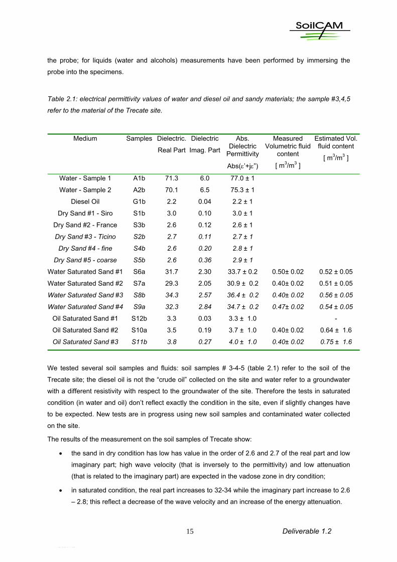
Table 2.1: electrical permittivity values of water and diesel oil and sandy materials; the sample #3,4,5

refer to the material of the Trecate site.

Medium Samples Dielectric.

Real Part

Dielectric

Imag. Part

Abs. Dielectric

Permittivity

Abs(’+j”)

Measured Volumetric fluid

content

[ m3/m3 ]

Estimated Vol. fluid content

[ m3/m3 ]

Water - Sample 1 A1b 71.3 6.0 77.0 ± 1

Water - Sample 2 A2b 70.1 6.5 75.3 ± 1

Diesel Oil G1b 2.2 0.04 2.2 ± 1

Dry Sand #1 - Siro S1b 3.0 0.10 3.0 ± 1

Dry Sand #2 - France S3b 2.6 0.12 2.6 ± 1

Dry Sand #3 - Ticino S2b 2.7 0.11 2.7 ± 1

Dry Sand #4 - fine S4b 2.6 0.20 2.8 ± 1

Dry Sand #5 - coarse S5b 2.6 0.36 2.9 ± 1

Water Saturated Sand #1 S6a 31.7 2.30 33.7 ± 0.2 0.50± 0.02 0.52 ± 0.05


Water Saturated Sand #3 S8b 34.3 2.57 36.4 ± 0.2 0.40± 0.02 0.56 ± 0.05


Oil Saturated Sand #1 S12b 3.3 0.03 3.3 ± 1.0 -

Oil Saturated Sand #2 S10a 3.5 0.19 3.7 ± 1.0 0.40± 0.02 0.64 ± 1.6

Oil Saturated Sand #3 S11b 3.8 0.27 4.0 ± 1.0 0.40± 0.02 0.75 ± 1.6

We tested several soil samples and fluids: soil samples # 3-4-5 (table 2.1) refer to the soil of the

Trecate site; the diesel oil is not the “crude oil” collected on the site and water refer to a groundwater

with a different resistivity with respect to the groundwater of the site. Therefore the tests in saturated

condition (in water and oil) don’t reflect exactly the condition in the site, even if slightly changes have

to be expected. New tests are in progress using new soil samples and contaminated water collected

on the site.

The results of the measurement on the soil samples of Trecate show:

the sand in dry condition has low has value in the order of 2.6 and 2.7 of the real part and low

imaginary part; high wave velocity (that is inversely to the permittivity) and low attenuation

(that is related to the imaginary part) are expected in the vadose zone in dry condition;

in saturated condition, the real part increases to 32-34 while the imaginary part increase to 2.6

– 2.8; this reflect a decrease of the wave velocity and an increase of the energy attenuation.

16 Deliverable 1.2

the soil samples, saturated with diesel oil, show a slight increase of the real part of permittivity

from 2.6 to 3.8 and a slight increase of imaginary part.

A more accurate estimate of the electromagnetic parameters could be obtained on samples of sandy

material, collected in the unsaturated zone (at the depth of 2-3 meters) in the not contaminated area.

The electromagnetic properties of the soil in different condition of fluid saturation (oil, water, water and

hydrocarbons) could be estimated on soil samples by using the fluid collected in the borehole in the

contaminated area at Trecate.

Preliminary electrical model of the contaminated zone - Trecate site The characterisation at laboratory scale permits to define a first electrical model of the most

contaminated zona at Trecate site; the model is shown in Table 2.2.

Table 2.2: electromagnetic parameters of the Trecate site

Depth Zone Electrical permittivity (real part)

Electrical permittivity (imaginary

part)

Electrical resistivity [ohm m]

Note

0-3 Silt with residual hydrocarbons

10-20 ? 50-100

3-7 Unsaturated zone 3-6 0.05-0.2 600 – 1000 7-10 “smearing zone” of

contaminated sand ? ? ?

10-12 Contaminated groundwater and effect of degradation

25-30 ? 80-150

12-18 Saturated sand and gravel

30-35 2.5-3.5 80-150

The model will be refined according to new laboratory tests, necessary to calibrate the georadar cross-

hole (in time lapse) and to obtain a more realistic model of the effect of the seasonal fluctuaction of

the water table that provides a “smearing zone” at Trecate site.

The soil is mainly compound by 80 % sand and 13 % silt and 7 % gravel and the smearing zone is

characterised by different saturation degree in water and hydrocarbons and by the intense activity of

biomass which determines a slow but continuous hydrocarbon degradation.

17 Deliverable 1.2

2.1.2 The Gardermoen site Here we refer to the information found in deliverable D2.1 and use part of that to interpret the

preliminary resistivity models (or their relative variations with regards to the reference model). Figure

2.2 shows the location of 6 points that core drillings with conventional ram drilling (RD) equipment

were carried out at the test field on Oslo airport, Gardermoen by FSU (Deliverable D2.1 by Markus

Wehrer et al., 2009).

A first sampling campaign was conducted at the runway of Gardermoen airport from Oct. 13th to 17th

2008. This campaign comprised screening with various geophysical methods (surface electrical

resistivity (ER) and surface ground penetrating radar, GPR), installation of electrodes for time lapse

resistivity measurements and invasive sampling with RD. From soil observations a lithological log was

generated for the 6 core drillings (RD1, RD3, RD5, RD7, RD9, and RD11) and one profile next to

lysimeter 8, containing main soil properties.

Figure 2.2: Location of RD points close to the time-lapse ERT lines.

We have used the lithological log presented in deliverable D2.1 to find links between the electrical

resistivity models and the lithological. Figure 2.3 depicts the lithological logs and water content

extracted from the soil samples taken by RD equipment in the locations shown in Figure 2.2.

According to deliverable D2.1 the upper 5 m underlying the test field at Oslo airport, Gardermoen can

be divided into 3 main units

- Layer 1: Ah horizon

- Layer 2: Bw horizon

- Layer 3: summarizes Cw, Bg, and Cr horizon that have redoximorphic features, illustrating the impact

of stagnant water and groundwater fluctuations.

The resistivity data presented here were collected along two lines of electrodes installed at 50 cm

depth as shown in Figure 2.2. The electrode cables were installed for time lapse measurements, in

this section however, we will use the initial data set acquired in December 2008. The shorter line (1)

with a length of 48 m is installed parallel to the runway in an almost NS direction and the longer one

18 Deliverable 1.2

(2) has a length of 96 m and has a NE-SW direction (Figure 2.2). A Wenner array configuration with a

minimum electrode separation of 1 m (see also deliverable D1.1) was used.

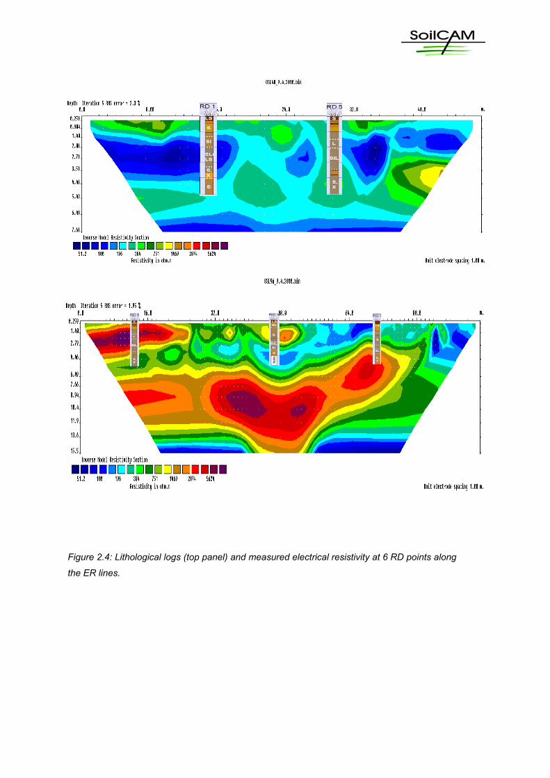
Figure 2.3: Lithological logs (top panel) and measured water content (bottom panel) at 6 RD points close to the time-lapse ERT lines.

We have superimposed the lithological logs on the inversion results of the electrical resistivity for both

lines. The line parallel to the runway (48 m long) is generally more conductive, this is most likely

caused by the effect of large quantities of de-icing chemicals infiltrating every year within the 30m

zone from the runway. The translation of the resistivity images to soil physical properties is

complicated because the soil profile is affected by de-icing chemicals. It is not possible to translate ,

Table 2.3 gives an overview of soil types with corresponding electrical resistivity based on a simple

comparison of soil cores displayed in Figure 2.3 overlaying electrical resistivites in Figure 2.4. If we

compare only for the unaffected areas i.e. outside the 30 m zone from the runway with the bore logs

we still see that the range of electrical resistivity values representing different grain size distributions is

large:

Silt: 200-700 Ohm m

Sandy loam: 200-300 Ohm m

19 Deliverable 1.2

Loamy sand: 200-400 Ohm m

Sand: 200-2000 Ohm m

Sandy gravel: 1500-4000 Ohm m

Table 2.3: Electrical resistivities signals compared to grain size in cores at the Oslo airport site

RD1 Electrical resistivity[ohm m] OSL48


Electrical resistivity[ohm m]

OSL96

RD3 Electrical resistivity [ohm m] OSL96


Sand 196-384 Sand 196-384 2874-5624

Sandy loam

196-280 Loamy sand

196-384

Silt /Loamy sand/Sandy loam

100-196 Loam - silt

196-280 1469-10000

Sand 900-2000 Sand 384-900

Sand - gravel

196 Sand gravel

280-650 384-751 Silt 196-650 Sandy gravel

1496-4000

Sand 196-280

20 Deliverable 1.2

2.2 The experimental design

The experimental design of geophysical survey requires close consideration of the objective of the

survey, the range of expected subsoil responses, acquisition costs, instrumental performance,

experimental conditions and logistics.

Figure 2.4: Lithological logs (top panel) and measured electrical resistivity at 6 RD points along

the ER lines.

21 Deliverable 1.2

2.2.1 The model framework The mathematical frameworks of experimental design are functions of the data and model spaces,

and are based on physical laws that connect the two spaces. The data space includes all parameters

that could be changed when acquiring data. For example, it may include all possible spatial locations

of sources and sensors, as well as characteristics of the field instrumentation such as frequency

range, source strength and receiver sensitivity. Although conceptually an infinite continuum, for

practical and numerical reasons the data space is usually discrete and limited. The main limitations

are the logistical problems, source and sensor positions that are usually restricted to the Earth’s

surface or few boreholes (ill-posedness) and the vector nature of the electrical and electromagnetic

fields that are often ignored in the experimental design.

The model space includes the range of possible subsurface structures and is continuous and

unlimited. Application of linearized inversion schemes usually requires the petrophysical properties to

be defined on finite cells or grids. A priori information, in the form of geological constraints and known

ranges of physical properties, imposes further restrictions on the model space.

In contaminated site characterisation, acquiring information on the subsoil electric and magnetic

properties is a critical task as in many geophysical applications. Since electromagnetic (EM)

geophysical methods are based on non-linear relationships between observed data and subsurface

parameters, designing experiments that provide the maximum information content within given a data

set of experimental data can be complex. Different approaches can be adapted to quantitative

experimental design: repeated forward modelling is effective in feasibility studies, but may be

cumbersome and time-consuming for studying complete data and model spaces; examining Fréchet

derivatives provides more insights into sensitivity to perturbations of model parameters, but only in the

linear space around the trial model and without easily accounting for combinations of model

parameters; a related sensitivity measure, the data importance function, expresses the influence each

data point has on determining the final inversion model; it considers simultaneously all model

parameters, but provides no information on the relative position of the individual points in the data

space; it tends to be biased towards well resolved parts of the model space.

The statistical experimental design is a more robust survey planning method, which is based on global

optimization algorithms, can be customized for individual needs and it can be used to optimize the

survey layout for a particular subsurface structure and is an appropriate procedure for non-linear

experimental design in which ranges of subsurface models are considered simultaneously.

The forward modelling and sensitivity analysis should be time consuming when 2D and 3D problem

are afforded, due to the model complexity and experimental data; we discuss the experimental design

strategy according to the global optimization theory. Global optimization theory is useful to examine

and rank different EM sounding survey designs in terms of model resolution as defined by linearized

inverse theory (e.g. Maurer et al. 2000). By studying both theoretically optimal and heuristic

experimental survey configurations for various quantities of data, it is shown that design optimization is

critical for minimizing model variance estimates, and is particularly important when the inverse

problem becomes nearly underdetermined. The concept of robustness is fundamental to define that

22 Deliverable 1.2

survey designs are relatively immune to the presence of potential bias errors in important data. Bias

may arise during practical measurement, or from designing a survey using an appropriate model.

2.2.2 Forward modeling of Slingram survey

Experimental design identifies the data acquisition arrangement (for example source–receiver

configurations, band width, acceptable signal to noise ratios) that ‘optimally’ determine a particular

subsurface model, with reference to the expected electromagnetic parameters of the Trecate and

Gardermoen site.

The main goal in experimental design of slingram broadband method with a fixed transmitter-receiver

distance is to:

verify the sensitivity in the adopted frequency band to the model parameters and

estimate the optimal frequency range that has to be adopted according to the fixed distance.

Figure 2.5: example of 1D modeling to analyse the parameter sensitivity on the observed data; a) reference model, b) configuration of the survey parameter; c) simulated noise d) synthetic geophysical response.

2.2.3 The 1D electromagnetic modeling of Trecate site

At this stage of the project, the reliability of the frequency domain electromagnetic investigation

(slingram survey) using a fixed coil distance device is estimated by means of the sensitivity analysis.

We consider a device with a fixed a distance coil and variable frequency; the theoretical response is

computed in the frequency range between 1 kHz and 100 kHz. The synthetic data were computed with

the CR1Dmod, a freeware forward modelling code in Matlab environment. We performed the modeling

of HCP FDEM (Horizontal Loop EM) with spacing of 2 meters between the two coils, which simulates

the operation of the Geophex GEM-2, used at the Trecate site.

With reference to the preliminary screening of the Trecate (see deliverable 1.1), a simplified model of

the sub-surface is defined, specifying the number of layers, the resistivity and thickness of each layer.

h1 , 1

h2 , 2

3

c

a

d

freque nc y

Sig

nal

h1 , 1

h2 , 2

3

c

a

d

freque nc y

Sig

nal

23 Deliverable 1.2

We defined a three layers’ model: a more resistive layer (some hundred ohm m) which simulates the

vadose zone, which is beneath a superficial conductive layer (pedological soil) and the conductive

lower half-space (saturated zone). The two conductive layers have resistivity value of 100 Ohm*m, the

superficial layer is 2 meters thick.

The sensitivity analysis has been performed by repeating the forward modelling and by perturbing the

thickness and resistivity of the intermediate layer, respectively from 5 to 9 meters and from 500 to 900

Ohm*m. Results are shown in Figure 2.6 and Figure 2.7.

Fig 2.6: Frequency depending response for different values of thickness of the intermediate layer, coil 1 refers to a thickness of the intermediate layer of 5 m; coil 2 of 7 m and coil 3 of 9 m.

24 Deliverable 1.2

Fig 2.7: Frequency depending response for different values of resistivity of the intermediate layer; a three-layer model is considered: the resistivity of the first layer is rho1=100 ohm m, thickness is h1=2 m; the resistivity of the second layer ranges rho2=[500 … 900] ohm m, h2= 7 m; the resistivity of the half-space is rho 3=100 ohm m.

The results (Fig. 2.6 and 2.7) point out that FDEM method with 2 meters spacing between the coils is

not sensitive to the resistivity values of the (more resistive) intermediate layer; the differences in the

response values at higher frequencies are indeed at the same order of the experimental uncertainties

(some ppm to 10-20 ppm). Better results can be obtained varying the thickness and resistivity values

of the superficial conductive layer, respectively from 1 to 3 meters and from 50 to 150 Ohm*m (Figure

2.8 and 2.9).

25 Deliverable 1.2

Fig 2.8: Frequency depending response for different values of thickness of the superficial layer

Fig 2.9: Frequency depending response for different values of resistivity of the superficial layer (resistivity 50 – 100 -150 ohm m)

The examples show the low sensitivity to the model parameters of the small coil distance system at

the frequency below 10 kHz; the sensitivity increases in the upper frequency limit; according to the

reduced coil spacing (2 m) the survey appears to be sensitive to the upper surface interface between

the conductive superficial layer and the second layer.

26 Deliverable 1.2

2.2.4 The statistical experimental design

We apply the statistical experimental design to optimise the data acquisition and process of georadar

cross-hole tomography, especially to the test site of Trecate; similar consideration yields for the

georadar experiments at Moreppen.

The basic idea of the statistical experimental design assumes that we may only acquire a fixed

number of data points: the suitability of such a data subset for interpretation can be examined using

any one of several diagnostics derived from linearized inversion theory (e.g. Curtis, 1999a for a more

detailed discussion and comparison of different approaches). Maurer and Boerner (1998) proposed a

suitability function (also called an objective function) based on the singular value spectrum of the

corresponding inversion problem:

[ 2.6]

where i are the singular values of a particular design, M is the number of model parameters and δ a

positive constant. This type of objective function can be minimized by avoiding data that lead to small

singular values, which, in turn, results in well posed inversion problems.

The −2 dependence makes the objective function inversely proportional to the a posteriori model

covariance (model accuracy), because minimizing this quantity is the ultimate goal of any experimental

design. The parameter δ is included for numerical stability in the presence of inherent non-

uniqueness.

The concept of avoiding redundancy in the experimental data that are dangerous in inversion

procedure can be applied to linearised inversion of cross-hole tomographic data (e.g. georadar data)

as discussed later.

As an alternative to the equation [ 2.6 ], the conditioning number of the linearised problem can be

adopted instead of the sum of all the singular value. The conditioning number is the ratio between the

maximum to the minimum singular value of the kernel of the linear or linearised problem.

In travel time tomography, if the assumption of the geometrical optic is valid, then the tomographic

problem is usually solved by dividing the space domain according to a pre-selected grid. In traveltime

tomography (seismic or electromagnetic), the optimisation procedure leads to estimate the “best

arrangement” of the cell along X and along the depth axis for the gridding used in forward modeling

and in the inverse inversion procedure, starting from a selected configuration of the transmitter (TX)

and receiver (RX) array. We avoid any considerations on the best arrangement of the TX and RX

arrangement using borehole georadar, because we consider a common good practice to collect data

with a spacing of 0.25 or 0.5 m, with some denser acquisition (0.1 m) where the most interested

features have to be investigated.

In travel time tomography, assuming a simple model of uniform soil (the electromagnetic parameters

are constant in the section between the two boreholes), a linear inverse problem has to be solved,

27 Deliverable 1.2

with M unknown (velocity distribution) and N equations (experimental data – travel times). The number

of equation is equal to the sum of all the TX-RX positions, while the number of model parameters (M)

depends on the cell size, in which the space domain is divided. The number of model parameters M is

the product between the cell along the distance axis (X-axis) and the cell along the depth axis (Z-axis).

The goal is to estimate the best combination of the cell number along X and Z that yields a good

compromise between the spatial resolution (cell size) and the reliability of the final solution (in this

case in terms of the disturbance of the experimental noise in the final model). As the decrease of the

cell size usually produces an increase of the ill-poseness and ill-conditioning of the problem, while the

increase of the cell size determines a more robust predicted model but a lack in spatial resolution

occurs.

By given a minimum and maximum value of pixels along X and Z axis, the main computational steps

are :

the contribute of each electromagnetic ray within each pixel for all the possible configuration of

the discrete grid; this permits the kernel of the linear system to be computed;

a singular value decomposition on the kernel permit to extrapolate the singular value vector

and the conditioning number (or in alternative the sum of all the singular values can be

performed, as required in formula [ 1 ]);

each element of the resulting matrix refers to a single combination of number of pixel along

the X and the Z-axis; the minimum values of the conditioning number identifies the “optimal”

combination of the pixel number that can be adopted in the tomographic process;

for the selected discrete grid, the bounds of the propagation of the experimental uncertainties

on the final solution of the model parameters can be predicted:

t

tk

M

M

.

where M is the space of the model parameters M is the uncertainties in the predicted model

parameters and t is the uncertainties on the traveltimes.

Example of optimisation of cross-hole radar data at Trecate site: At Trecate site the cross-hole radar data are usually collected in two boreholes (B-S3 and B-S4),

separated by a distance of 6 m and with a maximum depth of 17 m; a reasonable array of TX and RX

position is based on 25 source positions (spacing of 0.5 m) in the first borehole and 50 receiver

position in the second boreholes (spacing of 0.25 m). This arrangement covers the depth from 4 to 17

m, that is the most interesting zone for monitoring the change of the electrical permittivity within the

section between the boreholes.

The following simulation takes into account a number of pixel, which varies from 4 to 8 along the X-

axis and between 25 and 50 along the depth Z-axis . The cross-hole tomography yields an ill-posed

and ill-conditioned problem, where the conditioning number is usually very high (> 1000). We assume

28 Deliverable 1.2

that the problem is linearised, that it means to consider the straight line propagation of the

electromagnetic rays.

The plot of figure 2.10 shows the distribution of the conditioning number for all the possible

combinations of pixels (cells), according to the selected limits: higher is the value

Figure 2.10: map of the conditioning number of the cross-borehole data acquisition (Trecate site); the optimal choice of the pixel number along the two directions is given by the minimum values of the conditioning number.

29 Deliverable 1.2

Figure 2.11: example of distribution of singular values for a grid of 6 pixels along the X-axis and 30 along the depth axis; the lower singular values are indicative of the ill-conditioning in the inversion procedure.

The distribution of the singular value deals with an indication of the potentially more un-stable model

solution due to the propagation of the uncertainties of the experimental data. In the selected case, the

sharp decrease is noted for singular values lower than 4; therefore the model parameters (wave

velocity) associated at those cells can not be resolved in an accurate way.

2.2.5 Survey design of electrical resistivity tomography (ERT)

Resistivity imaging of the subsurface is based on the data sets collected using one or more of the

standard electrode arrays (e.g., the Wenner or conventional dipole-dipole array). During the last few

years, a significant effort in ERT prospecting has been done to develop techniques which obtain the

maximum information from each data set and at the same time reduce the amount of data which need

to be collected in the field.

Dahlin and Zhou (2004) computed the surveying efficiency (anomaly effects, signal-to-noise ratio) and

the imaging capabilities of ten electrode arrays over five synthetic geological models the pole–dipole,

dipole–dipole, Wenner–Schlumberger and gradient arrays appear the more suitable for 2-D resistivity

imaging. However, the mapping of the study area with more than one array types, which have different

theoretical and practical merits and demerits, can give different geoelectrical models. For example,

Wenner and Wenner–Schlumberger arrays appear to have high vertical resolution, while dipole–dipole

and pole–dipole arrays have high lateral resolution (Ward, 1989). Stummer et al. (2004) presented an

experimental design procedure to identify non-conventional suites of electrode configurations that

provide maximum subsurface information using a sensitivity based optimization scheme. They suggest

that combined data sets coming from different configurations carry more information than the

individual data sets.

30 Deliverable 1.2

The optimum electrode array configuration depends on the sensitivity to the target properties and the

propagation errors of the experimental uncertainties due to the inversion procedure.

Sensitivity

Furman et al. (2003) adopted the analytic element method to investigate the spatial sensitivity of

different electrical resistivity tomography (ERT) arrays. By defining the sensitivity of an array to a

subsurface location, maps are generated showing the distribution of the sensitivity throughout the

subsurface. This allows one to define regions of the subsurface where different ERT arrays are most

and least sensitive.

The comparison of three commonly used arrays (Wenner, Schlumberger, and double dipole) and for

one atypical array (partially overlapping) shows the limits of the double dipole survey compared with

the other surveys. A survey composed of a mixture of array types offer better performance to all of the

single array type surveys. This encourages us to develop an hybrid array configuration: a mixture of

Wenner and Schlumberger array is used in the surface data acquisition at the Trecate site.

Challenges in cross-hole data

A major source of uncertainty in cross-hole tomographic inversion is data error due to the electrode

mislocations; this is characterized by the sensitivity of electrical potential to both source and receiver

positions. This sensitivity depends not only on source–receiver separation, but also on the distribution

of the electrical conductivity in the investigated medium. In near-surface environmental and

engineering geophysical surveys, for which electrodes may be close to the target and experiment

dimensions may be on the same order as those of the target, errors associated with electrode

mislocations can significantly contaminate the ERT data and the reconstructed electrical conductivity.

The resulting perturbations of the reconstructed electrical conductivity field due to electrode

mislocations can be significant in magnitude with complex spatial distributions that are dependent both

on the model and the experiment.

The effects of geometric errors on cross-hole resistivity data are investigated using analytical methods

by Wilkinson et al, (2005); geometric errors are systematic and can occur due to uncertainties in the

individual electrode positions, the vertical spacing between electrodes in the same borehole, or the

vertical offset between electrodes in opposite boreholes. An estimate of the sensitivity to geometric

error is calculated for each of two generic types of four-electrode cross-hole configuration: current flow

and potential difference cross-hole (XH) and in-hole (IH). It is found that XH configurations are not

particularly sensitive to geometric error unless the boreholes are closely spaced on the scale of the

vertical separation of the current and potential electrodes.

It can be noted that extremely sensitive IH configurations are shown to exist for any borehole

separation; therefore it is recommended that: XH configurations be used in preference to IH schemes;

remove to filter out configurations with high sensitivities to geometric error to remove all the suspect

31 Deliverable 1.2

data; this filtering also significantly improved the convergence between the predicted and the

measured resistivities when the data were inverted.

Figure 2.12: Geometry of (a) cross-hole (XH) and (b) in-hole (IH) arrays for evaluation of general electrode position errors, and (c) XH and (d) IH arrays for evaluation of depth offset errors between adjacent boreholes. Current and potential electrodes are shown as open and filled circles respectively. Distances in (c) and (d) are given as multiples of the vertical electrode separation (after Wilkinson et al., 2005).

Figure 2.13: example of the sensitivity function of vertical section of cross-hole electrical resistivity pole-dipole array configuration on the region within the B-S3 and B-S4 boreholes at Trecate site using pole-dipole array (values are dimensionless); high values indicate a great dependence of the resistance measurement to the local variation of the model parameters; distances are in meters.

32 Deliverable 1.2

Figure 2.13 shows an example of the sensitivity analysis performed on the cross-hole data dealing

with the electrode configuration at Trecate site (24 electrode for each of the boreholes B-S3 and B-

S4). The image refers to the distribution of the sensitivity within the space domain (vertical section)

considering a pole-dipole array; measurements are distributed both according a XH scheme and the

in-hole scheme. The values indicates the dependence of the observed parameters (the electrical

resistance between the node of a pre-selected grid) to the values that the parameters assume at the

closer nodes of the grid. In a qualitative sense the sensitivity map is useful to optimise the grid cell

distribution, by considering a denser gridding close to the borehole where the sensitivity is maximum

and increase the cell size in the internal part of the space domain (low sensitivity). Following this

criterium, we adopt a non regular grid distribution in the data processing of the cross-hole data at

Trecate site.

Inaccuracy of the inversion of resistivity data

Some authors (e.g. Dehghani H. and Soleimani M., 2007) demonstrates the importance of accurate

modelling in terms of model meshing and shows that although the predicted boundary data from a

forward model may be within an accepted error, the calculated internal field, which is often used for

image reconstruction, may contain errors, based on the mesh quality that will result in image artefacts.

This encourage us to develop new modelling and inversion tools with an adaptive mesh as described

in the deliverable 4.1: this is relevant when geophysical data are used to infer the hydrological

properties of the soil (water content change) in time-lapse fashion.

Inversion of geophysical data enables to recover the best suited model parameters from the

experimental data. In 2D and 3D inversion the main procedure is mainly deterministic; the

deterministic inversion should be able to incorporate the propagation of the uncertainties and the a

priori information. This latter point is usually solved considering a bounded solution starting from

reference model parameter, inferred by the geological-hydrogeological model of the site or on the

basis of the results of geophysical logs and other surface geophysical investigations.

Combined inversion of data sets coming from different electrode arrays obtained over the same site

would allow us to combine the relative advantages of every array and thus to produce superior results.

de la Vega et al. (2003) presented combined inversion results of dipole–dipole and Wenner array data

obtained from a hydrocarbon contamination site. They suggested that combined inversion results have

superior depth of investigation and better lateral resolution when compared to the inversion results

obtained from each array separately. However, the use of 2-D combined inversion algorithm on

several data sets showed that some arrays dominate over others. For example, measurements

obtained using the dipole–dipole array have typically stronger sensitivity than measurements obtained

by the Wenner array. To overcome this problem a particular weighting factor can be applied to

equalize the participation of the data of each array. Since the sensitivity (Jacobian) matrices associate

variations in the model properties with variations in the observed data, the value of this factor uses the

Jacobian matrices which are produced for the data set of each array (Tsourlos, 1995).

33 Deliverable 1.2

2.3 Time-lapse survey

The time lapse data refer to the set up, acquisition, processing and relationship with the hydrological

soil parameters at the two sites.

At the Trecate site, the data sets discussed are :

Cross-hole investigation by using electrical resistivity;

Cross-hole and single hole georadar investigation.

In addition the Modelprobe teams are working on time lapse data collected along two preferential

profiles using electrical resistivity, polarisability and spectral induced polarisation at Trecate site; one

profile is within the most contaminated area, while the second one is a reference profile, located in the

un-contaminated area. These data are not discussed in this deliverable and will be integrated in future

reports according to the availability and data sharing with the Modelprobe consortium.

At the Gardermoen site the available data sets are:

Georadar investigation repeated (twice) on large area for soil mapping;

Time lapse electrical resistivity data along selected profiles.

At Moreppen the time lapse georadar data were collected to monitor the snow melt in spring 2009.

2.3.1 Time lapse surveys for cross borehole georadar The theoretical background of georadar (GPR) from surface and in cross-hole configuration has been

given in Deliverable 1.1. In the present context we only state that GPR method uses propagating

electromagnetic waves with frequencies above 100 MHz. In this frequency range, the propagation can

be approximated with ray theory, with Fermat’s principle determining the ray paths. Hence, the velocity

structure of the subsurface determines the ways the rays travel along and the time they need to do so.

The crosshole setting requires two boreholes, so that the receiver and transmitter can be in different

underground locations and different wave paths can be produced by varying source-receiver position

pairs. In cross-hole investigation, by measuring first arrivals, the ray paths as well as the velocity

structure can be inverted.

The propagation velocity of GPR electromagnetic waves is governed by the electrical permittivity () of

the host medium. Electromagnetic wave velocity and dielectric constant in soil are strongly influenced

by soil water content, because of the high dielectric constant of water compared to other materials (for

water is 80, while for common geological materials is in the range 5–15 and for air it is 1). The latter

can be directly converted into a dielectric permittivity distribution

rr

cv

with r being the relative permittivity of the material, c = 3.0·108 ms-1 is the speed of EM-wave in air and

the relative r magnetic permeability which is usually assumed to be 1.

34 Deliverable 1.2

The theoretical background behind radar wave propagation, the radar wave velocity and soil electrical

permittivity, and estimation of volumetric water content has been discussed by many authors (Topp et

al., 1980; Davis and Annan, 1989; Telford et al., 1990; Greaves et al., 1996; Reynolds, 1997; Hagrey

and Muller, 2000; Huisman et al., 2001; Huisman, 2002). The relative permittivity of Earth materials

generally lies between 4 and 10, while water has a high value of 81. Hence, the most important

parameter governing the velocity is the water content.

The measurement of wave propagation velocity or time lapse georadar data can be converted in soil

water content based on various relationships between water content and dielectric constant (e.g. Topp

et al., 1980; Topp and Ferré, 2002). The volumetric water content θ can be estimated by the empirical

Topp's equation (Topp et al., 1980).

Cross-hole geo-radar time-lapse measurements were conducted to investigate soil moisture

distribution and migration during infiltration process into the vadose zone. We monitored the vertical

distribution of electromagnetic wave by repetitive measurements using cross-hole geo-radar surveys

at Trecate and Moreppoen.

In crosshole GPR, two acquisition schemes are usually employed: the multi-offset gathering (MOG,

tomography geometry) and zero-offset profiling (ZOP, cross-hole geometry) (Binley et al., 2001). MOG

offers multi-dimensional imaging through high-resolution tomography, but data acquisition is relatively

slow due to the large number of measurements (Alumbaugh et al., 2002).

Tomographic schemes typically rely on some kind of ray approximation of the EM waves. Straight-ray

algorithms give reliable results if the velocity variations in the medium are moderate. If strong velocity

variations are expected, algorithms that take bending of the rays into account will produce more

reliable results. ZOP data do not require tomographic inversion, and the EM-wave velocity is

calculated for a known antenna separation, assuming that the first-arriving energy travels along a

direct path from the transmitter to the receiver. This assumption, however, can give rise to erroneous

velocity estimates if the traveltime of the refracted waves is lower than the direct wave traveltimes

(Huisman et al., 2003, Rucker and Ferré, 2003 and Rucker and Ferré, 2004).

By assuming a straight ray-path, a first arrival time is used to calculate velocity (v) as v = d/t, where d

is the offset distance between transmitter and receiver and t is the traveltime. By further assuming that

frequency-dependent dielectric loss is relatively small, the electrical permittivity is obtained from the

velocity values.

In porous media the time lapse cross-hole survey permit to estimate the EM-wave velocity changes

that are governed by the variations of the water content. The main source of uncertainties are related

to:

mislocatons and errors in the source-receiver positioning at different time step, because

usually the antennas are manually moved by the operator along the borehole;

uncertainties in the traveltime estimation;

35 Deliverable 1.2

error in simulation of raypaths and uncertainties due to the inversion procedure (MOG data

only);

bias introduced by the model used to convert the traveltimes into water content changes.

In ZOP investigation the first source can be neglected with respect to the importance of the other

sources, while in tomographic inversion the misleading in source-transmitter positioning could strongly

affect the final results, because of the ill-poseness and ill-conditioning of the cross-hole tomography.

2.3.2 Time lapse electrical resistivity The time-lapse electrical resistivity survey is based on the repetition of the electrical measurements at

different period using a fixed electrodes array configuration on the surface or surface and borehole

electrodes configuration. In contaminated site survey, the possible monitoring situations include

remediation progress at environmental, groundwater recharge, infiltration process.

The resistivity image is first recorded as "background" (before any dynamic process); after the initial

"background" setup, the survey is repeated at intervals in the same way (electrodes in the same place

using the same array type, etc.) so that any change of the soil resistivity can be detected. The time

lapse function uses the inverted background section when inverting the "new" section and the result is

usually presented as the difference between the two sections.

In interpretation of time lapse resistivity data, the bulk soil’s resistivity is related to the changes of the

soil’s saturation; porosity; and pore fluid resistivity by several semi-empirical relationship e.g. Archie’s

Law (Archie, 1941). The ratio of the bulk resistivity normalised with respect to the fluid resistivity is

related to the change of resistivity with time with the change of saturation according to the following

equation (e.g. French and Binley, 2004):

[ 3.1 ]

where the w and s are the fluid and soil resistivity, respectively, while t=0 refers to the observations

at the reference time. The exponent n is the cementation factor, accounting for the textural soil

condition; it’s an empirical coefficient: reference values range from 1.3 to 2.5.

2.3.3 Uncertainties in electrical resistivity interpretation In the conversion of resistivity changes to variations of soil saturation and porosity, a bias may be

introduced. In long term monitoring of the soil resistivity, the main critical aspects are related to:

1. it’s common to use a constant value for the n-exponent of the Archie law, which is considered

valid in the whole space domain of the investigated section or volume, while the cementation

exponent is not invariant in the space, as it depends on the soil texture; if at small scale (e.g.

laboratory experiments) the variation of the n-exponent is negligible, at field scale experiments

(meters or decade of meters) this assumption provide artefacts in the final interpretation of the

water content;

36 Deliverable 1.2

2. the fluid conductivity is affected by the ionic nature, concentration, mobility and temperature;

while the water conductivity could be estimated by water conductivity logs in the saturated

zone, the fluid conductivity within the pore space in the un-saturated zone could be affected by

the water that infiltrates from the surface with different and often unknown chemical and

physical properties, which changes in time and space;.

3. the effect of the surface electrical conductivity, which accounts for the electrical interaction

between the pore fluid and the solid grains, and depends on the distribution and degree of

clay particles, is neglected.

We analyse the effects of the first two items in the error propagation due to the model parameters

uncertainties.

Assuming that the water saturation increases from 0.5 to 0.8 (plus 60 %), for a reference values of

water resistivity of 25 ohm m, a variation of 10 % in the n-exponent value (from n=2 to n=2.2),

determines a decrease of soil resistivity of 66 % instead of 61 %, as predicted for a constant value of

n=2.

On the other hand, for a n-exponent equal to 2, an increase of pore water resistivity of 20 % provides

the decrease of the soil resistivity of 68 % instead of 61 %. This introduces an additional uncertainty

(in addition to the experimental inaccuracies) due to the sensitivity of the model response to the model

parameters.

37 Deliverable 1.2

3. Time lapse surveys at Trecate site The main objectives of the cross-hole investigation in the test site are:

to evaluate the effectiveness of the time lapse survey (electrical resistivity and georadar);

to monitor the “smearing” effect of the hydrocarbon due to the groundwater fluctuation; the

time lapse geophysical measurements should be focused on the search of the position of the

resistivity minimum, that could vary vertically with time, subject to the local hydraulic regime

which controls the frequency and the amount of recharge;

to monitor the infiltration rate in the un-saturated zone as consequence of infiltration forced

from the surface;

to establish relationships between the geophysical observed parameters and geochemical and

biological activity in soil and groundwater.

The data sets have been collected, starting from December, 2008, after a series of tests using

different electrical resistivity devices and several array configurations. The data acquisition was

conducted according to the following procedure:

set-up of two boreholes with PVC casing for groundwater monitoring and addressed with

electrode borehole; the boreholes were performed in the most contaminated area of the site;

tests of electrical cross-hole tomography using commercial available devices (Syscal R1 and

Syscal PRO) to check the repeatability of the measures and the reliability of the electrodes

coupling with the ground;

tests of the prototype POLARES for complex resistivity data acquisition in the frequency range

from 0.5 Hz to 130 Hz,

comparative tests between POLARES and commercial devices;

test of sensitivity of different cross-hole array configuration and time lapse data acquisition

(monthly);

test of repeatability and sensitivity to water content changes of georadar cross-hole

investigation (April, 2008);

time lapse georadar cross-hole and VRP measurement (monthly);

monitoring of physical and chemical parameters of the groundwater using a multiprobe device

(pH, temperature, dissolved oxygen, redox potential and water conductivity) to constrain the

data interpretation of geophysical data; the logs are repeated both in the boreholes in the

contaminated area (B-S3 and B-S4) and in some boreholes in the uncontaminated area;

continuous monitoring of the temperature, water conductivity and pressure level of the

groundwater in the borehole B-S3; the piezometric level at different times were used to

constraints the inversion of electrical resistivity data.

In such a context, we describe the results of:

38 Deliverable 1.2

1. tests of the prototype (Polares) for complex resistivity tomography in the frequency range

from 0.5 Hz to 130 Hz and comparison between the Polares performances and commercial

device results;

2. tests of repeatability and sensitivity of georadar cross-hole investigation to the water content

changes (April, 2008) and monitoring an infiltration test cross-hole radar.

3.1 Set up of the test site

The cross-hole investigation is based on the drilling of the two boreholes (B-S3 and B-S4) aligned in

west-east direction and located at a distance of 50 m in the eastern direction from the well B-I. The

two boreholes were drilled with conventional technology with a diameter of 127 mm, completed with

PVC piezometric tubes (blind from the depth of 6 meters to the ground surface). The maximum depth

of the boreholes is 18 m.

The internal diameter of 2 inches makes the couple of wells available for geophysical investigation

such as logs and georadar cross-hole survey. Each borehole is addressed with 24 graphite

electrodes, integrated along the cable; the electrodes are 0.7 m spaced, from the depth of 0.9 m to 17

m. The temperature, water conductivity and the groundwater fluctuations have been continuously

monitored in the well B-S3, starting from December, 2008.

The boreholes have been drilling in a zone of accumulation of silty material in gravel and sand

background as depicted in the figure 3.1; between the coordinate 50 m to 110 m a accumulation of the

finer material has been pointed out by surface georadar survey. The two boreholes, approximately

located between the coordinate 60-70 m, have confirmed the main stratigraphy and the presence of

contaminant in the vadse zone and as free phase above the water table (8-8.5 m).

39 Deliverable 1.2

Figure 3.1: georadar section (top) acquired with a 200 MHz antenna; bottom) interpretation of radar facies, according to the calibration of the drill core B-S1 and B-S3; Line 1 – W-E oriented. The section is W-E oriented. The borehole B-S3 is located at the coordinate 75 m

3.1.1 Borehole electrical resistivity

We discuss the main sources of noise of the electrical cross-hole tomography in the test site and the

results of time lapse electrical resistivity performed with the prototype Polares (see Deliverable 4.1 –

June 2009, for the technical parameters).

Time-lapse measurements with Polares started on September 2009 at the Trecate test-site. Cross-

hole ERT are conducted monthly in B-S3 and B-S4 with the device (Polares), acquiring data with a

Pole-Dipole array at different frequencies, respectively 0.45, 1.79, 7.15, 28.6 and 114 Hz.

RF1

RF2

RF3

RF4

RF1: radar facies 1, gravel, RF2: sandy-silt, RF3: gravel and sand, RF4:sand, RF5: gravel and sand

RF1

RF2

RF3

RF4

RF1: radar facies 1, gravel, RF2: sandy-silt, RF3: gravel and sand, RF4:sand, RF5: gravel and sand

50 m

40 Deliverable 1.2

Figure 3.2: zoom of the zone of ERT1 and cross-hole investigation at Trecate

Inversion of resistance data is carried out using ProfileR2 (by Andrew Binley, Lancaster University,

ModelProbe Consortium), which give an inverse solution for a 2D resistivity distribution based on a

regularised objective function combined with weighted least squares (Occam’s type).

The adaptive finite element mesh is thickened around the boreholes, where the sensitivity analysis

gives the highest values (see section 2), wider cells are distributed in the middle of the investigated

section test, and also out of the region delimited by the two piezometers.

3.1.2 Noise sources The preliminary evaluation of the data quality has been performed by acquisitions using dipole-dipole

configuration array with about 1200 and 1400 measures (04-12-2008 and 13-01-2009) with a IRIS

Syscal R1 equipment.

The evaluation on the data quality reveals that:

only one electrode, the number 18 in borehole S3, is affected by coupling defects;

all the electrodes below the water table have low electrode contact resistances (0.7 kohm);

the average value of the contact resistance of the electrodes above the water table is about 3

kohm, with a maximum level of 10 kohm in the electrodes close to the ground surface.

This implies a low disturbance on the measurements referring to the central core of the section and do

not provide relevant noise in the processed section. The comparison between the results of the cross-

hole tomography (04-Dec-2008) and the surface ERT (27-Oct-2008) is showed in figure 3.3.

41 Deliverable 1.2

Figure 3.3: top) ERT 1 – resistivity model from surface measurements, the dash box is zoomed at the bottom; bottom) comparison between the cross-hole resistivity section; middle) with the zoomed part of the resistivity model (left); the resistivity values are in log10 scale in ohm m; left) soil column (Geoprobe) up to the depth of 13 m; S: silty soil SSH; silty-sand with hydrocarbon, SGH: sand gravel and hydrocarbon; GS: gravel and sand; SG: sand and gravel.

The quality of the resistivity and chargeability data are validated according to the following protocol:

check of the contact resistance of each electrode;

during the data acquisition, the array-sequence was optimised to minimise the probability of

the electrode polarisation effect by avoiding the use of the same electrode previously adopted

as the current, as the potential electrode as better explained in the following;

all the data affected by errors greater than 10 % with respect to the average value of the

observed resistance, as measured by 3-6 cycles of current injection, was exterminated as bad

datum;

finally, the homogeneity of each distribution function and the similarity between the probability

distribution function of the resistivity value and chargeability value are evaluated; this permit to

detect the presence of singularity anomalous data that have to be removed before to invert the

data set.

The main sources of noise in the polarisability measurements in using the multielectrode devices

(borehole) are the capacitive effect, the electromagnetic coupling and electrochemical effect on the

electrodes.

The capacitive coupling in the cables is likely to be relatively stable and it decreases quickly with

increasing distances between the transmitting cables and the potential reading cables. In time domain

measurements, it is often assumed that the inductive coupling between the cables via the ground

mainly influences the data quality at earlier times and that it quickly decreases; it is convenient to

-2 0 2 4 6 8 10-18

-16

-14

-12

-10

-8

-6

-4

-2

0

Distance [ m ]

De

pth

[ m

]

-2 0 2 4 6 8 10-18

-16

-14

-12

-10

-8

-6

-4

-2

0

p[

]

Distance [ m ]

2

2.5

3

GW L

42 Deliverable 1.2

consider the decay curve only after a certain delay (Sumner, 1976). The voltage decay was integrated

starting from a time of 50 – 100 ms after the current turn-off.

The signal is often weak and much lower than the direct current potential, which is itself sometimes

small compared to the charge-up effect potential measured on the electrodes that have previously

been used to inject the current (Dahlin, 2000). The adopted instrument (Syscal Pro, Iris Instrument)

was characterised by a high resolution voltmeter and a powerful transmitter; at the same the

POLARES prototype was designed with a high impedance, high resolution and a powerful transmitter

(250 W).

A charge can appear on the potential electrodes if the potential electrodes have previously been used

to transmit a current. In such a case, a strong potential, much higher than the direct current potential

itself, can take several tens of seconds or some minutes for the charge-up to be discharged. In

resistivity surveying, we avoid this effect by using a plus-minus-plus type of injection current cycle (at

least 3 cycles); to obtain accurate chargeability measurements, the potential electrodes were not used

only after some minutes later that the electrodes have been used to transmit a current (e.g. Dahlin

2000).

Electrochemical phenomena might provide a charge at the potential electrodes (e.g. Vanhala and

Soininen 1995), if non-polarisable electrodes are usually used. The use of graphite or stainless

electrodes and multicore cables for DC resistivity measurements, appears possible, at least in

favourable conditions (Dahlin et al, 2002).

3.1.3 Constrains Inversion is constrained by the definition of a three-layers model of sub-surface, assuming a reference

model that is derived from the geological setting of the area and from the surface electrical

investigation.

The superficial layer is set with a thickness of about 2 meters and a resistivity of 100 Ohm*m, the

intermediate layer with variable thickness and resistivity around 800 – 1000 ohm m which corresponds

to the vadose zone, where the bottom of the layer is the groundwater level, and a lower half-space

having resistivity value of 100 Ohm*m (saturated zone). In order to estimate the resistivity values an

independent data set of resistivity value was used, observed with a in-hole configuration (dipole-

dipole).

3.1.4 Results Time-lapse survey was conducted at several frequencies in order to check the presence of frequency

effect on the collected data sets (results are not yet available); in such a context we only discuss the

changes of resistivity distribution from the data acquired at the frequency of 1.79 Hz. The regular grid

between the boreholes used in the inversion process has about 500 elements.

43 Deliverable 1.2

The results are plotted in figure 3.4; the water level seasonal fluctuaction is also indicated on the

sections (dashed line).

Fig. 3.4: cross-hole electrical resistivity tomography (borehole S3 and S4), acquisition at 1.79 Hz using the Polares prototype; left) image at 09th September ’09, middle) image at 15th October ’09; right) image at 09th November ’09 (distance are in meters).

The resistivity of the upper conductive layer slightly change over time with a decrease of resistivity

value from September to November, 2009, while the resistivity values of the intermediate layer are

increasing. This should be related to the change in time of the groundwater level with a reduction of

the water content within the the vadose zone due to the effect of the capillarity.

A preliminary conversion of resistivity values was performed by applying Archie’s law to the resistivity

value of the interpreted sections. For each elements the ratio of the saturation value is calculated from

the Archie’s law, assuming a saturation exponent equal to 2, as assessed by laboratory investigation

on the selected soil samples (see section 2)..

The value of the water conductivity is known from the chemical-physical monitoring; this value is

supposed to be constant for each panel; the water conductivity values of 0.041, 0.05 and 0.057 S/m

are observed at September, October and November (2009) respectively.

44 Deliverable 1.2

Figure 3.5: trend of the water conductivity (Sp Cond), redox potential (ORP) and dissolved oxygen (DO) at different time period, arrow an horizontal black lines indicate the groundwater oscillation in the most contaminated zone.

The plots of figure 3.6 reveal the water conductivity changes at different periods; it remains

substantially constant with depth. The similar behaviour is shown by the redox potential and the

dissolved oxygen. In contrast the values are more stable for different periods of acquisition in the logs

performed in the borehole outside the contaminated area e.g. water conductivity is about 400

microS/cm). The degradation of hydrocarbon, that is still active as indicated by the low values of the

dissolved oxygen, affects the electrical conductivity of groundwater in different way according to the

seasonal behaviour of the groundwater level or according to the contribute of the water from the

surface infiltration. Therefore the interpretation of the electrical tomography has to consider the

change in time of the water conductivity also.

45 Deliverable 1.2

Fig. 3.6: Time-lapse analysis of the saturation changes as estimated from electrical resistivity data left) saturation ratio between data set of October, 2009 versus the data of September, 2009; right) saturation changes between the data of November, 2009 data versus September, 2009.

The ratio of the saturation values, referred to those of September; are shown in Figure 3.6; the values

greater than 1 represent the increment of saturation, while values lower than 1 represent a decrease

of the water content; the phenomenon is related to the water-table oscillation, the surface infiltration

and evapo-transpiration effects that are not yet considered. The dashed lines represent the

groundwater level in October and November, while the point-dashed lines indicates the groundwater

level (September, 2009).

The red zones of the images (figure 3.6) point out the decrease of the saturation, while the blue zones

indicate the part of the section which is interested by a decrease of the water content.

In the panel of figure 3.6 which refers to the image of October versus September, the principal

increase of the saturation is concentrated in the upper part of the image and at the depth of about 6-7

meter, just above the water level. A slight decrease of saturation (value below of 1) in the zone

between the two groundwater levels is also observed. Below the groundwater level (October), a slight

average increase of the “apparent” saturation is observed. As we are referring to the saturated zone

the effect of the uncertainties in the conversion of resistivity changes in saturation changes are clearly

evident. These effects are also observed in the second panel (November versus September data),

where below the groundwater level artefacts in the estimate of the apparent saturation are depicted. In

the intermediate zone, between the two groundwater levels, the decrease of saturation is on the order

of about 30-40 %.

It can be noted that the time-lapse investigation provides reliable results as far as concerning the

coherence of the electrical resistivity variation in time, with a complex behaviour in the vadose zone ;

this process should be connected to the saturation and re-distribution effects, which is related to the

46 Deliverable 1.2

lowering of the groundwater level from September to November and to the infiltration process from the

surface.

The saturation changes within the saturated zone appear biased by the application of the relationship

between the electrical resistivity and saturation. The application of simple constitutive relationship

(Archie law) to convert the change of resistivity in saturation changes with time appears to be

unrealistic or at least very complex to interpret. For instance, it can be noted a marked increase of the

saturation (at November) just above the groundwater level, that cannot be easily explained.

3.2 Georadar time lapse data

The spatial and temporal distribution of water content was derived from velocity estimates based on

the standard ZOP (zero offset profile) method that assumes that all the first-arrivals of the

electromagnetic wave are due to a direct propagation. However, critical refractions can occur

whenever EM waves travelling through a low-velocity medium reaches a boundary with a higher-

velocity medium. If the GPR antennas are located within a high water content layer that is adjacent to

a lower water content layer, critically refracted waves may arrive before direct waves. Although critical

refractions cannot be distinguished from direct arrivals on a single radargram, they exhibit identifiable

behaviour on a traveltime profile. The traveltime of a critically refracted wave can be shorter than that

of a direct wave if the measurement is taken close to the boundary between two layers of contrasting

dielectric permittivity (Rucker and Ferré, 2003 and Rucker and Ferré, 2004). This mainly occurred if a

sharp electrical interface is related to the groundwater level and therefore is connected to the water

retention curve of the soil. In finer material, where vertical gradual variation of water content (and

therefore of the permittivity) is expected, the errors introduced by critically refracted waves are

negligible.

3.2.1 ZOP data acquisition

The data acquisition has been repeated monthly using a Pulse EKKO radar system equipped with two

separated antennas at the main frequency of 100 MHz. Measurements were collected in a cross-hole

configuration with a spacing between two adjacent stations of 0.25 m. Additionally data were acquired

in vertical radar profile configuration using the same equipment with the transmitter on the surface and

moving the receiver antennae along the borehole with a spacing increment of 0.05 m.

47 Deliverable 1.2

Figure 3.7: April, 2009; left) GPR raw data and correlation with the main soil stratigraphy; right) example of water content estimate inferred by cross-hole (ZOP) data acquisition and conversion of electrical permittivity using the Topp formula. The groundwater level was at depth of 8.5 m.

The figure 3.7 depicts the results of traveltime picking of cross-hole GPR data, collected in the

boreholes B-S3 and B-S4 (April, 2009 at Trecate site); the water content has been computed

according to the Topp formula; the accuracy in water content estimate is governed by the accuracy in

traveltime picking and the bias in the model of conversion in water content.

The smoothed vertical profile shows a gradual increase of the water content with depth. An abrupt

change of the water content should be expected at the depth of 8.5 m, where the groundwater level

was locate at the acquisition time; that is not revealed by the data, .A gradual changes of the water

content in the saturated zone is due to the soil porosity changes with depth.

3.2.2 Analysis of time lapse data of April, 2008

An infiltration test was performed in April, 2009, in the area addressed with the two boreholes B-S3

and B-S4. The total volume of water injected into the soil was 2 m3 requiring approximately 5 hours for

all water to flow out. A constant hydraulic charge was applied; as injection point a vertical PVC liner

inserted in the upper layer to 2 m in depth was used.

The preliminary estimate of the water content just below the injection point (depth of 2m) was inferred

by TDR measurements; an average wave velocity value of about 0.09 m/ns was observed just below

the injection zone, at the beginning of the experiment.

Time-efficient ZOPs were utilized because relatively fast water migration into the sandy-gravel layer

was expected. In ZOP mode, both transmitter and receiver antennas are lowered to a common depth.

ZOP measurements represent horizontal averages of EM properties between boreholes at different

depths. GPR data were collected every 0.25 m at depths of 1 to 18 m. It required approximately 15

min to cover the whole depth range. The measurement series were repeated several times in the first

Critically refracted wavesfrom the air-ground surface

Silty and Sand (dry)

Capillary fringe zone in sandy soil dielectic is sensitive

to water content

Transiction zone (Refracted rays) effects of biomass, void clogging …

Low radar velocity(Saturated) high watercontent zone

Critically refracted wavesfrom the air-ground surface

Silty and Sand (dry)

Capillary fringe zone in sandy soil dielectic is sensitive

to water content

Transiction zone (Refracted rays) effects of biomass, void clogging …

Low radar velocity(Saturated) high watercontent zone

48 Deliverable 1.2

two days from the beginning of the injection (April, 23th). A total of 12 acquisition were performed

during the experiment that lasted for some days.

The results are summarised in the figure 3.9. The plot shows the change of water content at different

times (x-axis) in the depth range from 1.5 to 5 m (y-axis); the scale value indicates the water content

changes in m3 on m3. The Topp formula was used to convert wave velocity (or electrical permittivity) in

water content.

Figure. 3.8: image of water content changes, inferred by georadar time lapse data, during the infiltration test; acquisition step refers from time 0 (beginning of the infiltration) to 5 days later (acquisition step 8); data are converted into water content change using the Topp formula; step 1= 40 min after the start of infiltration; Step 2= 80 min; Step 3= 150 min; Step 4= 20 h; Step 5=22 h; Step 6= 24 h; Step 7= 3 days; Step 8= 5 days after the infiltration. The values are in m3/m3.

The saturation process in the upper part of the subsoil proceeds very fast; the infiltration and the

redistribution of the water mainly occurred along the horizontal direction (time); the maximum effect

that can be collected occurred at a depth of about 2-2.5 m from the surface. The water content

increases at the top in the first acquisition step appears strongly over-determined; this could be

partially due to the inaccuracies due to the critical refraction of the electromagnetic wave at the

interface between the wet zone and the “dry” zone.

The experiment permitted to check the good sensitivity of the method to the water infiltration, the low

vertical permeability of the upper surface layer and the preferential distribution of the water along the

horizontal direction. This agrees with the presence at the depth of 2-4 m of a low permeability silty

level which minimise the impact of the vertical flow in the area. At the final stage of the experiment

(after 5 days from the beginning of the infiltration), a residual high water saturation still appears at the

depth of 2 m from the ground surface. We associate this effect to the latter effect of water

redistribution at the interface between the sandy and gravel upper layer and the lower silty low

permeable layer. Unfortunately, we couldn’t check this effect for latter times because of the

interference of the infiltration form the ground surface due to the intense rainfall, which occurred after

few days from the beginning of the experiment. This is responsible for the partial redistribution of water

A c q us itio n s te p

De

pth

[ m

]

1 2 3 4 5 6 7 8

-4 .5

-4

-3 .5

-3

-2 .5

-2

-1 .5

-0 .1

0

0 .1

0 .2

0 .3

0 .4

0 .5

0 .6

0 .7

49 Deliverable 1.2

just on the near surface layer, with an increase of the water content as pointed out at the step 7 and 8

of the data acquisition (Figure 3.8).

3.2.3 Attribute analysis of GPR signature

Despite recent technological advances, the majority of current GPR applications focus on event

location and mapping only, with limited effort being applied to the extraction of material property

information (e.g., volumetric saturation extent, etc). Through the use of attribute analysis methods it is

possible to obtain additional information on the nature of the sub-surface materials directly from the

GPR data (i.e., by analysing the spatial variation in signal attenuation, wave velocity, etc). However,

these particular properties must be directly related to the macroscopic dielectric parameters of the

contaminating fluids (i.e., the permittivity and conductivity spectrums) before GPR attribute analysis

methods can be considered suitable for practical use. Cassidy (2004), by combining the direct

dielectric measurement of NAPL contaminated materials with numerical simulations of GPR wave

propagation, demonstrated the frequency dependent behaviour of GPR signal attenuation and velocity

variation across a range of typical NAPL related problems.

The contaminated ground waters have a significantly higher attenuation rate (loss tangent) when

compared to the ‘clean’ ground waters. This is consistent with the observations that the dissolved and

biodegraded phases show increased electrical conductivity. Consequently, GPR signal attenuation is

likely to be increased in areas where dissolved phase products are present in the water table and

capillary zones.

Therefore, time lapse cross-hole data should be useful to monitor the NAPL behaviour if attenuation

analysis could be performed together with traveltime analysis. For instance, the spectral analysis of

ZOP data could be used to estimate the attenuation parameters in the saturated and the unsaturated

zones. Moreover the effect in cross-hole or in VRP data of the hydrocarbon contaminants just above

the water table (smearing zone) can also be detected. The presence of contaminant should provide

more sensitive effect in frequency domain analysis than in time domain because for instance the

phase rotation of the signal at the interface between the clear and the contaminated zone. At this

stage of the project we’re working on the amplitude spectra more than on the phase analysis.

As far as the attenuation is concern, in cross-hole survey (ZOP) the following equation yields:

rtTTdd

dEE exp0

0

where d is the distance between the transmitter and receiver in the two boreholes, E and E0 are the

signal amplitude at the receiver and transmitter respectively, and is the attenuation coefficient

(Np/m), Tt and Tr are the transfer functions at the receiver and transmitter antennas. By assuming that

the Tt and Tr are constant in air-filled boreholes and they change when the antennas are located in

the water-filled part of boreholes, the ratio between the amplitude spectra in the saturated zone with

respect to the saturated one is:

50 Deliverable 1.2

rt

srstss

TT

TT

d

d

E

E ,,

exp

exp

where the symbol s refers to the values in the saturated conditions;

rt

srsts

s

TT

TTdd

E

E ,,loglog

The equation can be re-written as:

KdKdd ss

Therefore the ratio R of the amplitude spectra between the saturated and un-saturated zone is related

to the difference of the attenuation coefficient in the saturated and un-saturated zones.

The following example provides a comparison of the analysis of traveltime and spectral data; in the left

panel of figure 3.9 the first arrivals are converted in to wave velocity while in the second panel the

peaks of the amplitude spectra at different depth in the cross-hole data (ZOP) collected in December,

2009 and April, 2009 are plotted.

With reference to the figure 3.9, the wave velocity gradually changes in the unsaturated zone to the

depth of 9 m (groundwater level); at level below the water table the wave velocity continues to

decrease till the depth of 12.5 m, due to the effect of critically refracted waves: in the transition zone,

just when the antennas are located below the water table, the velocity refers to an apparent velocity.

The differences between the trend of November with respect to December is mainly related to a

decrease of the water content in the vadose zone. This affects the contrast of the electromagnetic

properties above and below the water level, with a consequence on the traveltime of the critically

refracted waves.

51 Deliverable 1.2

Figure 3.9 : Trecate site – cross-hole radar investigation in the boreholes B-S3 and B-S4 ; left) wave velocity trend in November (red line) and December, 2009 (blue line) ; right) peaks of the amplitude spectra (red – November, 2009, blue – December, 2009). The dashed line indicates the groundwater level in November, 2009, the dot line in December, 2009.

The data in frequency domain (right panel of figure 3.9) show three different zones: in the upper part

of the unsaturated zone, the peaks of the spectra are close to the values of 80-90 MHz, while the

nominal frequency at the source was 100 MHz; in the saturated zone the average value is about 50-55

MHz ; in the intermediate zone, the peaks gradually increase from the minimum to 80-90 MHz. In this

zone the response is very sensitive to the different saturation conditions due to the groundwater

fluctuation and the different distribution of the water below the groundwater level between November

and December 2009, as depicted in the right panel of figure 3.10.

The dispersive effect of the electromagnetic waves with depth is related to the changes in the

electrical conductivity between the saturated and the vadose zone; this analysis could be useful to

relate the effect of hydrocarbon degradation within the smearing zone.

52 Deliverable 1.2

Figure 3.10 : Trecate site, acquisition 2009; radar ZOP, temporal evolution of the traveltime and the centroids of the amplitude spectra

53 Deliverable 1.2

4. Time-lapse surveys at Gardermoen Geophysical surveys both GPR and DC (electrical resistivity) were conducted at two sites at

Gardermoen; Oslo airport and Moreppen. At the Oslo aiport site, both methods are reported, while at

the Moreppen site, we only report the results of the GPR time-lapse measurements. DC results will be

reported later.

4.1 Time-lapse GPR survey at Oslo airport

We performed two GPR surveys at Gardermoen site, Oslo airport: the first one was conducted at

October, 2008, the second one was performed in July, 2009 (13-15).

The two surveys were organised to investigate an area of 200 m x 200 m close to the runway, using

GPR device in single reflection mode, equipped with an antenna operating at the main frequency of

200 MHz. The two surveys were carried according to a grid-based criteria; due to the arrangement of

the profiles the two data set can be compared in a robust way only in the North-East portion (100 m x

100 m), close to the runway.

We acquired high density sampling interval measurements on the 100 x 100 m area in order to

generate time-slices of the reflection amplitude of the radar signals.

Figure 4.1: Scheme of the acquisition of the GPR survey – October, 2008; the hatched area refers to

the100 m x 100 m area that has been investigated in detail; the magenta arrow refers to an additional

54 Deliverable 1.2

radar profile, collected along the same transect of the electrical resistivity section discussed in the text.

The time-slice or depth-slice technique is used in many GPR applications to provide a spatial (in

pseudo-horizontal plane) representation of the reflection amplitudes, usually acquired along parallel

profiles. The time-slice technique allows one the amplitude reflections, due to the buried

electromagnetic discontinuities, to be reconstructed through horizontal sections at different time of the

acquisition window (that in some way can be converted in depth). The technique is highly valuable in

detecting buried cavities and archaeological features (Orlando, 2007; Berard and Maillol, 2008) and in

mapping soil heterogeneity. The time-slices allow the implementation of 3D modelling, thus facilitating

the identification of the location of the principal detected features.

The procedure to generate the timeslice is summarised:

1. the GPR data are collected at high density sampling interval along straight parallel profiles, in

one or more directions;

2. the GPR data are geo-referenced in a local or global reference system;

3. each single profile is processed according to a standard flowchart of data processing;

4. the absolute value of the radar reflection amplitude are stacked on a selected time-window,

the size of the time window is tuned to the main pulse period of the radiated signal.

5. the amplitude are interpolated on a regular grid to generate 3D regular matrices of “reflectivity”

at different times;

The process leads to the generation of 2D maps at different time; by estimating the velocity of

propagation of the radar signal it is possible to refer the maps at different depths.

Data Positioning

The data positioning of radar survey is done using a Global Positioning System (GPS), which is

directly linked to the central unit of the georadar and is moving with the radar antennas. A second

GPS receiver is used as a fixed station elsewhere close to the surveyed area; it operates as a base

station for the correction of geographical data.

The first survey was performed with a single frequency GMS-2 receiver with an external antenna

located on the radar antenna. Data were acquired along straight parallel profiles spaced 2.5, 5 and 10

m apart both in East-West direction and in North-South direction. The length of the profiles was 100 m.

Additionally, a survey wheel device, mounted on the radar antenna, drove the GPR acquisition. A

serial cable linked the GPS receiver to the radar controller, sending the standard GGA format as

NMEA output to the pc. GGA is an essential fix data which provide 3D location and accuracy data. It

provides information such as Coordinate Universal Time (UTC), latitude, longitude and elevation, GPS

quality, numbers of available satellites etc. The GPS receiver was set to receive EGNOS corrections,

but during the survey they were not available. Therefore the survey of October 2008 the GPS device

worked in stand-alone way, performing absolute positioning of the radar traces. The data were

collected in a short time (two nights); in open space without obstacles between the satellites and the

receiver: this permitted a good local reference system data to be collected. The relative position

55 Deliverable 1.2

between data had a good accuracy (few decimetres), while the data positioning in a global reference

system has low accuracy (some meters). Figure 4.2 shows the positioning of the data.

Figure 4.2: GPS track of the first survey at Gardernoen (Oslo airport), data October, 2008.

During the second survey we adopted two double-frequency Leica 2400 GPS receivers with external

antennas; one as the base station and second one, mounted on the radar antenna, acted as the rover.

A special set up of the GPS receivers permitted to sent the corrections at the frequency of 1 Hz (RTK)

from the base station to the rover during the acquisition. In this case, the accuracy in the positioning of

every radar trace on the local reference system was of few decimetres, as the position of the base

station was georeferenced without any corrections. An accuracy of few centimetres of the global

positioning system is obtained after the post-processing of the data of the static base station with the

Oslo GPS permanent station (OSLS), with known coordinates (DGPS mode). The difference between

the corrected and the un-corrected position of the base station has been adopted for applying a

translation to all the rover data (Fig. 4.3). The final data set has the same accuracy both in horizontal

coordinates and elevation.

56 Deliverable 1.2

Figure 4.3: GPS track of the second survey at Gardermoen (Oslo airport), July, 2009

The new topographic survey permitted to acquired the topography of the area; the data set can be

used to perform the static corrections to the georadar data.

The georadar survey of July, 2009 served to demonstrate that in geophysical kinematic applications:

1. it is not necessary to know in advance the coordinates of the base station, that can placed

elsewhere close to the surveyed area;

2. it is possible to obtain real time data with high accuracy in a relative positioning system,

avoiding time-consuming post-processing;

3. it is possible to obtain high accuracy data on a global reference system post-processing

just the static base station, and applying a rigid translation to all the rover data.

The suggested procedure avoided the use of the survey wheel device for controlling the georadar

acquisition, permitting to speed up the acquisition process using a motor vehicle for moving the

antenna on the investigated area (Annex A).

4.1.1 GPR data processing The data processing permitted time-sections to be reconstructed, geo-referenced in UTM WGS84.

They pointed out several reflection features in the depth range approximately up to 5 meters.

57 Deliverable 1.2

The radar data, acquired in the sub-area AA (100 m x 100 m), close to the runway/landing strip, were

processed to elaborate the time-slices of “the reflected amplitude” by using a time window of 5 ns, on

a grid of 0.05 x 0.05 m. The time-slices were computed in the range between 0 ns and 200 ns. To

make easier the comparison of the results, the same reflectivity amplitude range was used for all the

time-slices. A natural logarithmic scale has been adopted, to enhance the dynamic of the parameter

response. Each time-slice was converted in depth-slices using a wave velocity of 0.07 m/ns; this value

has been estimated by the diffraction hyperbola analyses of the radargrams.

The second survey allowed a larger area to be investigated in the same working time as the first one,

because of the use of a small tractor for towing the antenna. A static correction, which takes into

account the topographic effect (correction of the traveltimes due to the difference in elevation for

different position of the radar antennas). Except for the static correction, the same data processing

flow chart was adopted on the data set acquired in July, 2008.

The tilting correction takes into account the horizontal and vertical components due to the effect of the

topographic slope gradient on the signal radiation. These corrections are relevant when the inclination

of the slope angle is above 6-8º. We didn’t consider these corrections because of the gently slope of

the investigated area. Anyway, in the next future we would explore the effectiveness of the dynamic

corrections as a further improvement in time-slice data quality. In order to apply the dynamic

corrections to georadar data the accuracy of the horizontal coordinates and elevation should be of

1/10 of the wavelength (Lehmann and Green 2000). In such a case, an average wave velocity of 0.07

m/ns and a main frequency of 200 MHz yields to a wavelength of 0.35 m which requires an accuracy

of 3.5 cm in the global positioning. This accuracy cannot be addressed by RTK acquisition with the

post –processing of GPS data (DGPS).

4.1.2 Results We compare the stratigraphic evidence with the radar section, performed in October, 2008. The radar

line is aligned along a NE towards SW direction; it is 140 m long. The 0 m coordinate is close to the

runway (Fig. 4.4).Three boreholes were drilled along the same alignment, reaching a depth of 5 m.

58 Deliverable 1.2

Figure.4.4: position of the radar line for comparison with the stratigraphic columns; the blue line refers to the radar line AF discussed in the paragraph (acquisition October, 2008)

The figure 4.5 depicts a vertical section of a radar profile along the line plotted in magenta in figure 4.4

(survey, October, 2008). The comparison with the main results of the stratigraphic evidence (see

deliverable 2.1) is also shown. A wave velocity with a constant value of 0.07 m/ns has been assigned

all along the section. The main reflection features depict some gently dipping layers with an apparent

inclination from NE towards SW, which is accordance with the sedimentary setting of the area. The

groundwater level at the time of the survey was about 7 m below the surface.

From a qualitatively point of view, a good agreement with the stratigraphic evidence is observed: the

main reflection between the sandy and silty soil shows a gently slope from NE to SW; a different water

retention behaviour of the soil (see deliverable 2.1) indicates an increase of the water content in the N-

E part, close to the runway. This could be responsible of the high signal attenuation in this sector, as

well depicted in the time slices, discussed in the next paragraph.

59 Deliverable 1.2

Figure 4.5 comparison of GPR section and borehole data along the NE-SW profile; data acquisition October, 2008.

4.1.3 Time-lapse survey The slices (see Annex A) permit to verify:

the data quality is acceptable to a depth of about 5-6 m from the surface;

the data are spatially well correlated at least up the depth of 4-5 m;

some effects due to the surface features, such as the runway/landing strip, are clearly visible;

The main features are aligned in the depth-slices along NW– SE direction; these features are related

to the large-scale buried morphology; as a preliminary interpretation, the features, characterised by

higher relative amplitude, could be associated to the coarse sediments, while lower amplitude are

related to finer sediments.

On the eastern side, close to the runway/landing strip, the signal amplitude appears strongly

attenuated with respect to the western part of the investigated area; this effect is mainly evident in the

depth-slices between 3.5 m up to 5 m, and could possibly be influenced of the infiltration of the de-

icing chemical compounds which might affect the soil conductivity, providing an increase of the

attenuation of the radar amplitude.

The results of the second survey (July, 2009) show a general similarity in the detection of the main

features with the data of the previous survey; some differences in the absolute reflection are depicted

in the two periods; they can be associated to:

the different coupling between the antenna and the ground surface because a different

electromagnetic behaviour of the uppermost layer in the two seasons (wet in winter and dry in

summer):

a different distribution of the water content in the vadose zone could affect the propagation

and reflection behaviour of the signals.

NE SW

High water content

Loam silt

Sandy

Silt

Loam

NE SW

High water content

Loam silt

Sandy

Silt

Loam

High water content

Loam silt

Sandy

Silt

Loam

60 Deliverable 1.2

4.2 Time-lapse DC-resistivity measurements at Oslo airport

Changes in electrical resistivity in the soil profiles at Oslo airport are caused by the

following effects:

- Temperature changes; during snowmelt situation changes from frozen ground to

temperatures well above freezing, this will reduce the electrical resistivity in the

ground

- Snowmelt infiltration; up to about 1m of snow with an equivalent water amount of

200mm is stored throughout the winter and infiltrates during the snowmelt. This

will increase the saturation levels in the soil and hence reduce the resistivity

- Presence of de-icing chemicals in the melt water; Potassium Formate (KFo) is

an organic ion used at runways during winter time. Increased electrical

conductivity of the infiltrating water in areas where snow is affected by the

chemicals will also cause a reduction in electrical resistivity

To separate between these effects is impossible without additional measurements of

these processes. For practical reasons only the two top meters are monitored for

changes in these values, i.e. soil temperature, water content and electrical conductivity

of the fluid phase. The top 2 m are however most affected by these factors.

A series of Electrical Resistivity measurements were conducted using multi-electrode instrument

(SYSCAL Pro) during the period March to June 2009. Preliminary a modelling has been performed

using the Res2dinv code. The electrical resisivity (ER) data were acquired along two profiles, (1)

running in parallel to the runway with a length of 48 m in an almost NS direction and (2) had a length

of 96 m in a NE-SW direction (Figure 4.6). A Wenner array configuration with a minimum electrode

separation of 1 m (see also deliverable D1.1) was used.

61 Deliverable 1.2

Figure 4.6: Aerial photo from the western runway of Gardermoen; the measured Syscal resistivity lines and the Ohmmapper lines are indicated as red lines.

The two lines intersect Hydra Probes (Stevens Water Monitoring systems) that were installed at 0.25,

0.5, 1 and 2 m depth. These sensors monitor water contents, electrical conductivity and temperature

of the soil and will be used for interpretation of time-laps measurements to study changes in electrical

resistivity. Table 4.1 contains the information about the data acquisition along both lines. The first

measurements were carried out on 11/03/2009 and are referred to as the reference data.

Table 4.1: Dates of ERT data acquisition along lines 1 and 2 after the reference measurement on

11/03/2009.

Line 1 20/03/0

9

01/04/0

9

14/04/09 23/04/09 04/05/09 19/05/09 29/05/09 22/06/09

Line 2 14/04/09 23/04/09 04/05/09 19/05/09 29/05/09 22/06/09

Days

after

ref.

9 21 34 43 54 69 79 103

4.2.1 Inverse modelling results The measured time-lapse ER data have initially been modelled with the Res2dinv software. Default

values for model discretisation and no conditioning was used in the inversion process, hence the

results are of preliminary character. The data collected 11/03/2009 were used as reference data set or

initial conditions. The reference data set is included as the first dataset, while later measurements are

62 Deliverable 1.2

presented as the relative changes to the reference model. Figure 4.6 show the modeling results along

line 1.

Figure 4.6 2D reference model of ERT resistivity data along line 1 measured 11/03/2009 (topmost left panel) together with the percent change of the six time-lapse data. The number to the right bottom of each section shows the measurement number referred to number 1.

As was shown in chapter 2, there is a contrast in resolution between the measurements

of electrical resistivity and the groundtruthing method of analysing core samples. The

same is the case with calibration with field measurements of temperature, water content

and electrical conductivity of the fluid phase. While the inverted resistivity images

provide a resolution in the order of 0.5 to several meters, measurements with the

Hydraprobes give point values. In view of the likely presence of preferential flowpaths,

it is highly likely that the overall changes seen in the inversion results are not

represented exactly by the point measurements. This will be discussed further in the

next section. Alternatively to calibration with field measurements, changes in electrical

conductivity as a function of temperature, water content and electrical resistivity can be

measured in the laboratory (described in chapter 2). This has been done (although not

63 Deliverable 1.2

for temperature) for soil from Moreppen, but not yet for soil from Oslo airport.

Information will be provided in later reports.

Results of the timelapse measurements along line 1 (48 m long) are shown in Figure

4.6. The reference model (sampled 11/03/2009) is referred to as 1, and the last date is number

7 (22/06/2009). The change in resistivity from 1 to 2 shows relatively small changes (light green,

around a few ohm m) except the layer at the depth of about 1.5 m. At this depth there is a

positive resistivity change compared to the reference model. The maximum reduction in

resistivity (about 30%) occurs below approximately 3m, which is somewhat surprising

since the most changes are expected near the surface where infiltration occurs. The

presence of an impermeable membrane below the soil surface stretching out to about

7m from the runway, to a depth of about 2.7 m could have an influence on the deep

layer changes. The changes in 3-1 show the same increase in electrical resistivity at the

same depth as in 2-1. Apart from that feature, the entire profile shows a reduction in

electrical resistivity of up to a maximum of 70%.

Figure 4.7: 2D reference model of ERT resistivity data along line 2 measured 11/03/2009 (topmost left panel) together with the percent change of the six time-lapse data. The number to the right bottom of each section shows the measurement number referred to number 1.

The differences between 1 and the rest of the measurements (3-1 to 7-1) shown in Figure 4.6 remain

almost the same with some minor changes implying that the resistivity of the medium is rather stable

64 Deliverable 1.2

and unaffected. This is in line with previous experimental work at Moreppen (French et

al., 2001), where water was held at field capacity after the all the snow had infiltrated.

Results of time-lapse measurement along line 2 are shown in Figure 4.7. Also for this line

there is a zone where resistivities increase. In this profile the increase in resistivity is

found deeper than along line 1 and at about 6 m depth. The groundwater level in this

area is about 6m below the surface near the runway (the 0.0 point of line 2) and about

7 m near the end of line 2. If these measurements represent real changes in water

contents in the profile, they might be explained by finer material on top of courser

material, but this needs to be confirmed by deeper ground truthing in the area. Artifacts

in the inversion process also need to be checked further. Similarly as for line 1 most

change in the profile occurs between 11/03/2009 and 14/04/2009. The vertical blue

feature at about 30 m from start marked by a red arrow in the model difference shown in Figure

4.7, could indicate a zone of preferential flow or focussed infi ltration. This effect has

been documented by previous measurements at Moreppen (French and Binley, 2004)

and by observations of ponding at the soil surface at Oslo airport.

4.2.2 Hydra Probes data, Oslo airport At the intersection of the two lines, Hydra Probes were installed to register the temperature, water

content and electrical conductivity of soil. Data from the period 11/03/2009 to end of July 2009

(with exception of 29/04/2009 to 14/07/2009 with missing data replaced by linear interpolation)

are shown Figures 4.7 and 4.8. The soil water content is measured with the time domain

reflectrometry which only measures fluid water content, frozen soils may therefore see

an artificial increase in water content when the soil ice melts and becomes fluid.

Starting with the uppermost sensor at 0.25m depth, negative temperatures are

measured until some days before 11/04/2009, the water content increases almost

simultaneously, but since also the electrical conductivity of the water increases, it

seems likely that most of the increase represents real changes in water content. This

means an increase of about 0.1 in volumetric water content. The second probe at 0.5m

depth, shows a similar pattern only some days delayed compared to 0.25m. The initial

water content is higher than above, but could be an effect of temperature closer to 0ºC

hence more fluid water, or a finer grained soil. At 1m depth water contents increase

before the soil temperature and the increase occurs prior to the response at 0.5m,

again this might be an effect of soil heterogeneity and the presence of preferential flow

paths. Even at 2m depth the water content response is very similar in timing to the

sensor at 0.5 m, again preferential flowpaths may explain and also the effect of piston

flow, since the electrical conductivity does not change in the two deepest points,

although changes of EC can’t be measured at these levels of water contents. For all

depths there is a fast increase in water content followed by a somewhat slower

decrease. Water contents at all depths return to initial values towards medio-July. The

65 Deliverable 1.2

sudden increase in water contents at 11/04/2009, corresponds well with the reduced

resistivity in the ER lines, compare Figures 4.6 and 4.7 – difference between reference

day and time 2 and 3. The relative increase in water content ranges from 150 to 600%

at the specified depths.

Figure 4.8 Measured water content, conductivity and temperature of soil at 0.25 m (left) and 0.5 m (right).

66 Deliverable 1.2

Figure 4.9: Measured water content, conductivity and temperature of soil at 1m (left) and 2m depth (right).

67 Deliverable 1.2

4.2.3 Slingram measurement at Oslo airport A set of measurements in Gardermoen airport were carried out by Majid Beiki from Uppsala University

in July 2009. The instrument used for the measurement was CM031 that belongs to POLITO. It

measures the electrical conductivity of the ground at low induction number using coplanar vertical

magnetic dipoles. The frequency used was 9.766 kHz and the instrument has a transmitter-receiver

separation of 3.74 m. The data were acquired along the same profiles measured with the OhmMapper

instrument by Bioforsk (see Figure 5.6). In order to be able to transfer the data from the instrument, a

special connection is needed. The hardware also belongs to POLITO and at the time of measurement

it was not at our disposal. Unfortunately because of some delay in deliver the instrument to Polito (due

to custom troubles during the shipping of the instruments from Norway to Italy), the internal memory of

the instruments was cancelled and that data were lost.

4.3 Experiments at the Moreppen site

Data were acquired at Moreppen, near Oslo aiport, Gardermoen in Norway by Majid Beiki (Uppsala

University) with an instrument rented from the Norwegian geotechnical institute (NGI). Moreppen is a

test site that is has a geology similar to the airport site (Deliverable 2.1, and French et al., 2001,

French et al, 2004). Hence we assume measurements at Moreppen are valid for extrapolation to

similar processes at the airport. The geological environment consists of glacial sediments, mostly

sands and gravel. The groundwater table lies at approximately 4 m depth. Two pairs of boreholes (EF

and CD) were drilled through the vadose zone (see Figure 4.1) down to the groundwater table.

Borehole separation was 2.2 m. The boreholes are located next to a trench that has been dug before

in order to characterize the site. The distances to the trench are 1.4 m for boreholes EF and 1.8 m for

CD, respectively.

Before the starting of the thaw period in April, the snow was removed and de-icing chemicals (either

Potassium Formate, KFo or Propylene glycol, PG) was applied onto the soil surface. After recovering

the area with snow, the thawing period was monitored from 2009-03-31 until 2009-04-18 with repeated

GPR crosshole measurements in each pair of boreholes. The measurements took place every second

day, resulting in 10 surveys per borehole pair. The goal of the measurements was to study

propagation of water and contaminant into the subsurface.

68 Deliverable 1.2

Figure 4.1: Borehole positioning in Moreppen in relation to the trench.

4.3.1 Data acquisition In each pair of boreholes, a receiver and a transmitter were moved to every position between 0 and 5

m depth with 0.10 m increments. In some cases the instrument failed when brought below the

groundwater table, so data reach only to 4 m depth. This gives 51 (or 41) source and receiver

positions. For all possible permutations between source and receiver position a radar trace has been

recorded. Thus, every day 2601 (1681 with 4 m depth respectively) traces were collected. The

sampling rate of the instrument is 5.12 GHz, so each sample represents a time interval of 0.19 ns. The

central frequency of the instrument is 250 MHz, giving a wavelength of 0.4 m for a electrical

permittivity value equal to 9. The spatial resolution is usually regarded as no more than a quarter of

that.

4.3.2 Data analysis In this section, the raw data processing and problems encountered are discussed. Visualization and

processing was carried out with Claritas software. The processing consisted mostly of resorting and

reformatting the data sets, removing the static zero time, as it was recorded before and after

conducting the measurement in a pair of boreholes. The zero times remained stable over the whole

study at a value close to 2 ns.

The instrument used in this study consists of a single receiver and a single transmitter antenna. The

source remained at a fixed position while the receiver was moved. Hence, the error of source position

is static for every source gather, while the receiver positioning error is random. In the receiver gathers,

both errors are random. Consequently, receiver gathers are noisier than source gathers (see Figure

4.2). This could be avoided by the use of a multi-channel receiver device.

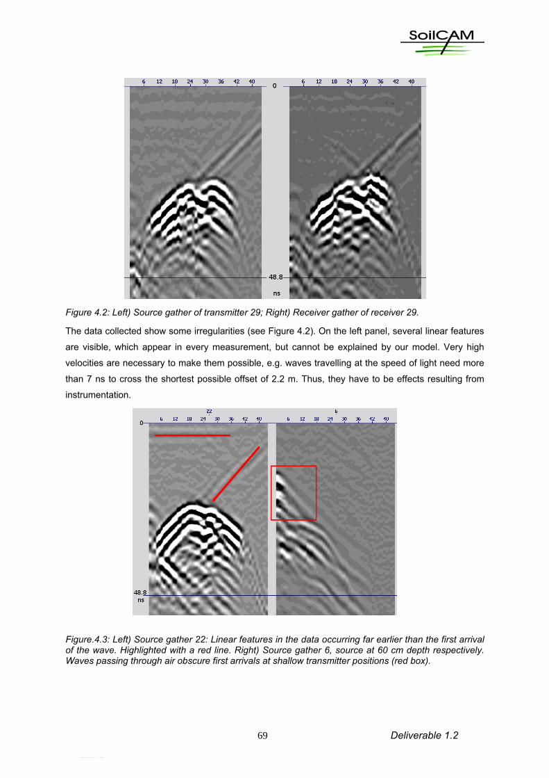
69 Deliverable 1.2

Figure 4.2: Left) Source gather of transmitter 29; Right) Receiver gather of receiver 29.

The data collected show some irregularities (see Figure 4.2). On the left panel, several linear features

are visible, which appear in every measurement, but cannot be explained by our model. Very high

velocities are necessary to make them possible, e.g. waves travelling at the speed of light need more

than 7 ns to cross the shortest possible offset of 2.2 m. Thus, they have to be effects resulting from

instrumentation.

Figure.4.3: Left) Source gather 22: Linear features in the data occurring far earlier than the first arrival of the wave. Highlighted with a red line. Right) Source gather 6, source at 60 cm depth respectively. Waves passing through air obscure first arrivals at shallow transmitter positions (red box).

70 Deliverable 1.2

Especially the diagonal feature very often tends to obscure valuable information when it interferes with

the shortest offset first arrivals which can in that case no longer be picked reliably.

In the right panel, the source is close to the surface at source position 6 (60 cm depth). The strong

influence of an air wave, that travels out of the borehole, over the ground and down the receiver’s

borehole. Since the wave velocity is very high in the air, receivers and sources close to the surface

can measure these waves as the first arriving ones. This obscures the direct wave travelling through

the medium that provides the desired velocity information. Hence, first arrival picking is not possible

there.

The proximity of the trench made it necessary to assess the possibility of its effect on the first arrivals

of waves that, instead of travelling through the investigated subsurface volume, take a faster path

through the trench and thus can be picked as the first arrivals. A 3D modeling was performed with

Pstomo_eq6.6.1 program (Benz et.al.1996, Tryggvason 1998). We used a homogeneous half-space

of 0.9·108 ms-1 as a reference and calculated the difference to travel times coming from the same

model with a trench (an air-soil interface parallel to the borehole array) with varying distance. The

velocity was chosen as a lower limit to the observed velocity. The differences would only decrease

with increasing velocity. The first arrival travel time variations from the model without trench in percent

are displayed in Figure 4.4. The largest offsets between receiver and transmitter are affected most.

For a distance of 1.8 m, even the largest offsets are not noticeably affected. Hence for data from the

boreholes CD the 2D assumption is not affected by the trench. For 1.4 m, however, only offsets lower

than 3.5 m are free of distortion. Thus, in the interpretation of boreholes EF, the affected data was not

taken into account.

Figure 4.4: Absolute difference (in percentage) of first arrival travel times between a homogeneous half space of 0.9·108 ms-1 and models with a trench parallel to the borehole pair computed for different distances of the air-soil interface.

71 Deliverable 1.2

For robustness it was decided to pick on the first strong amplitude arriving, not on the very first onset

of the waves, since the latter very often is drowned in background noise. The wavelet of the

instrument as it was recorded at zero-offset is displayed in Figure 4.5. It is not a minimum phase

wavelet - the second maximum is the one with the strongest amplitude. Hence, it is possible that

under bad noise conditions the wrong maxima were picked, introducing systematic errors.

Figure 4.5: Wavelet recorded at zero-offset.

Examples of travel time picks are shown in Figure 4.6.

Figure 4.6: Travel times picked from various exemplary source gathers; trace number on x-axis (from

top to bottom of borehole ?) and traveltime along the y-axis.

The data collected in boreholes EF show a remarkable transition from a strong maximum, denoting

the first arrival, towards a strong minimum as first arrival at the deeper receiver positions with numbers

> 24. This change of phase is open to interpretation at the moment. This transition is observed for the

source gathers 17 to 32 in Figure 4.7. Over all 16 displayed gathers, a discontinuity at around receiver

72 Deliverable 1.2

24 is visible. At depths (receiver >35, 3.5m), a zone of sudden higher velocity becomes apparent.

Figure 4.7: Data of boreholes EF for sources between positions 17 (1.7 m) and 32 (3.2 m), from right to left and top to bottom . Observe an amplitude discontinuity and a revolution of the phase evolving at receivers with number >24 (2.4 m deep) while the transmitter moves downwards. The maximum of the first arrival becomes a minimum.

73 Deliverable 1.2

4.3.3 Inversion The inversion was carried out with Pstomo (eq.6.6.1). This code for 3D forward and inverse modelling,

but can handle 2D data sets and models likewise was originally developed by Benz et. al. (1996) and

further developed by Tryggvason (1998). .

The inversions were performed independently for every model. The starting models used were

obtained by taking the velocities from travel times between receivers and transmitters at the same

positions. Regarding these times as arrivals of horizontally travelling waves, the starting model

obtained is a layered model. This was done for most models individually. Only the first three data sets

from CD share the starting model obtained from the third data set in the way described above.

Individual starting models make it much easier to fit the data, since a shared starting model is

differently far from the truth for all data sets. However, for the first two data sets from CD, only a few

horizontal shots could be picked reliably, so no good starting model could be created. Figure 4.8

shows an example of the observed data (picked first arrival times) and the simulated data after the

inversion.

Figure 4.8: Observed data (left) and simulated data after iteration 6 (right) for measurements in the boreholes EF on 2009-04-18.

4.3.4 Results Results of the inversions of the data of CD are displayed in Figure 4.9 and for EF in Figure 6.10. The

wave velocity distribution between the boreholes is displayed. The results for CD share data fits of 0.5-

0.6 ns.

74 Deliverable 1.2

After the snow melt, a significant decrease in velocity down to 0.9·108 ms-1 in the upper two parts of

the model can be observed on 2009-04-06. It is associated with an increase in soil moisture due to

melting water intrusion. The lower velocities propagate further downward and on 2009-04-12 almost

all higher velocity features have vanished. After that, the velocities starts to increase again, indicating

a decrease in the water content. The velocity increases first where there have been higher velocities

before. This trend of stabilization continues until the end of the measurement at 2009-04-18. The

results for EF have slightly worse data fits of around 0.6–0.8 ns (3–4 samples).

The snow began to melt at around 2009-04-04. The models for earlier measurements that are very

similar as it is expected. These models can be regarded as the models unperturbed by changes in soil

water content. In CD the structure can be roughly described by four regions: a velocity of around

1.0·108 ms-1 down to 1.2 m depth. Between 1.2 and 2 m the velocity is around 1.1·108 ms-1 to 1.15·108

ms-1. From 2 m down to 3-3.5m velocities are highest at between 1.2·108 my layer at 2–2.2 m shows

itself. The suggested water infiltration and dehydration of the various zones happens at different

speeds. The high velocity zone below 2 m appears to be less permeable than the upper parts of the

model, since it takes several days until a significant decrease can be observed. On the other hand, the

rapid velocity increase in these zones from 2009-04-14 onward suggests a lower water retention

capability, with the exception of the zone between 2 and 2.2 m.

The unperturbed models of EF share the low velocity zone down to 1.2 m. However, below this a more

inhomogeneous picture is obtained. Roughly described, the area between 1.2 m and 2.5 m is of higher

velocities, similar to CD, but from there downward the velocities decrease. Directly after the snow

melting period starts, the most observable decreases in the velocity take place in the surface area and

between 2.5 m and 3 m. The lower part of the model differentiates into a very low velocity part, that

suggests an increase in soil water content, and a localized high velocity feature at around 3.5 m and 4

m depth. This feature is not always at the same position. It appears to be an inversion artifact, but as

pointed out above, the data indicate higher velocities in this area. However, no good explanation for

this feature can be presented without further investigation. The area between 1.2 m and 2.5 m also

shows a decrease in velocity, but as observed in CD, it happens later, and reverses earlier.

75 Deliverable 1.2

Figure 6.9: Inversion results of data at borehole pair CD.

Figure 4.10: Inversion results of data at borehole pair EF.

76 Deliverable 1.2

5. Recommendations

We summarise the main objectives of the application of geophysical methods in the two test sites as

follows. Particularly we would:

detect the main soil heterogeneities at the field scale (Oslo airport) and at local scale

(Trecate and Moreppen);

establish robust relationships between the geophysical response and the soil properties

such as porosity, water content and hydraulic conductivity to constrain the flow and

transport model in vadose zone;

optimize the time-lapse survey to detect the distribution of contaminants in soil and

groundwater and analyse the temporal effect of soil-contaminants reactions.

We pursue the aforementioned statements according to the optimisation of field survey mainly

based on frequency domain electromagnetic methods, georadar from surface and borehole, (complex)

electrical resistivity from surface and boreholes. We are focussing to improve the relevance in the best

design of the geophysical survey, the importance of including a priori information and physical

constraints, according to the soil properties, to improve the reliability of the geophysical data

processing.

5.1 Soil heterogeneity

High resolution and high accuracy in mapping soil heterogeneity can be obtained by using GPR

survey with RTK GPS positioning; the method is effective to map the soil heterogeneity on large scale

for a preliminary assessment of the presence of coarse and finer sediments at Osl airport; according to

the electromagnetic properties of the site is realistic to map the soil sediments to a depth of 5-7 m from

the surface.

The georadar investigation at Osl airport revealed the importance of an accurate geo-referencing of

the single radar trace if the soil mapping heterogeneity would be recovered in a reliable way and if the

data set collected at different periods should be compared each to other. The required accuracy in

spatial positioning is achieved using a GPS survey with two-linked GPS devices: one linked to the

radar antenna and the second one located elsewhere on the site. This permitted the application of the

topographical data correction to achieve an accuracy of some centimetres. High accuracy is

necessary if the static correction have to be applied for taking into account the ground topography.

Moreover, is not the case of Trecate and Ols test sites where the ground surface is characterised by

gently slopes and flat areas, the application of dynamic correction for reducing the effects of antenna

tilting should be explored when accurate time lapse investigation is necessary.

77 Deliverable 1.2

5.2 Experimental design

The experimental design has been focused on the analysis of the frequency domain investigation and

in the resistivity tomography survey.

A preliminary analysis states the low resolution of the slingram survey according to the electrical

properties of the Trecate site and the selected intercoil distance and frequency (1 kHz – 40 kHz) The

methods appears sensitive to the changes of the electrical resistivity of the upper surface layer and to

the depth of the interface between the top soil (pedological soil and the soil that has been interested

by soil remediation - up to 2 m in depth).

Moreover the sensitivity analysis checked, that according to the target properties and the noise level

(of Trecate site), the data collected at frequency higher than 20 kHz are more suitable for detecting the

change of the soil resistivity.

The optimum design of the slingram investigation has to be investigated to select the optimum

frequency range and the intercoil spacing with emphasis to the target properties and experimental

uncertainties. The sensitivity analysis states that the resistivity changes of the upper surface layer in

the order of 20 % provides change in the quadrature response of some decades of ppm, which is in

the range of the experimental uncertainties. This states that as the method should be suitable for the

reconnaissance of the hot spots or for soil mapping (heterogeneities), it doesn’t appear suitable for

monitoring temporal changes due to the soil moisture variations.

As far as concern the electrical tomographic approach, the advantage of the use of mixed

configuration array to increase the spatial resolution and to minimise the impact of the propagation

error into the final solution was explored. The redundancy of the experimental measurements should

increase the ill-conditioning of the inversion procedure due to the inclusion of singular values in the

kernel matrix. An accurate post-processing to the data is necessary before the inversion process by

attenuating the negative of the lower singular value.

The optimum data acquisition of the cross-hole tomographic survey has been explored by testing

several electrode configurations; we conclude that at Trecate site the optimum acquisition is achieved

using the in-hole scheme and the pole-dipole; this array guarantees a good compromise between the

stability and repeatability of the experimental measurements and the sensitivity and the resolving

power.

5.3 Data inversion

The main activities are focused on the analysis the best strategies to incorporate a priori information

in the inversion of single panel and the experimental uncertainties in cross-hole resistivity and

georadar tomographic data. An useful strategy is to include a priori information on the cross-hole

resistivity data, taking into account a simplified stratigraphic model and bounding the soil resistivity in

the saturated soil according to the water conductivity derived by logs.

78 Deliverable 1.2

We have made some preliminary attempts to run a joint inversion of ERT and RMT data collected at

Trecate site. Because of incompatible data format of the acquired data with the modeling program we

could not succeed to prepare such results. We are in contact with Dr. Thomas Kalscheuer from the

ETH University in Zurich to overcome the problem. The first trials with single inversion runs on the

ERT data have produced reasonable results and we are going to present some results of the joint

inversion in the next deliverable (24 months report). We are also preparing the 3D codes to model the

Trecate RMT data. In parallel the 3D inversion of ERT data using Res3Dinv will be carried out and the

results will be compared to the RMT model.

5.4 Time lapse data

The Trecate time lapse experiments (georadar data) have pointed out the great sensitivity and good

accuracy of georadar data to analyse the temporal water content change that it can useful to

characterise the infiltration rate from the surface and to analyse the saturation-desaturation effect due

to the seasonal water oscillation. The infiltration test confirmed the presence of a less permeable (silty

medium) layer at the depth of 3-4 m from the surface that governs the water flow at deeper level. This

observation agrees with the presence of a relevant residual contamination of hydrocarbon in the soil,

detected at the depth of 3-4 m (B-S3 and B-S4).

Tests of electrical tomography: and sensitivity analysis have permitted to arrange a pole-dipole array

configuration for stable and robust cross-hole resistivity measurements at different time steps. The

inverted sections of cross-hole data appear to be well related to the lithology and to the vertical

(averaged) water content, inferred by the cross-hole georadar survey. We’re confident that more

detailed analysis on the properties of the material will be available when the resistivity data, acquired

at different frequencies will be inverted. Moreover we are trying to incorporate in the inversion

procedure the information of water content distribution, inferred by cross-hole GPR.

An attempt to convert the resistivity into saturation variations in time has been done using simple

Archie model. This appears to be realistic at laboratory scale on sandy materials, while appear to be

un-effective when applied on field data. Secondary effects due to the local changes of water

conductivity, temperature effect and not-ionic electrical conductivity should be considered.

At Moreppen site, the preliminary tests have shown that the snow melt and the associated melting

water intrusion could be detected with the crosshole GPR measurements; whenever the goal of

differentiating between contaminant and water wasn’t achieved. A rough picture of the velocity

distribution could be obtained but the detailed features in models are highly doubtful.

Especially the further examination of the hydrological parameters of the subsurface at the site could

be improved if ERT measurements were also provided and a joint interpretation was carried out.

For a more qualitative interpretation of time variations of the medium we need to carry out

measurements of electrical resistivity and radar signal between the boreholes at the same time

especially during the snowmelt period.

Since the Gardermoen airport is a very noisy area we have planned to make a perusal check of the

acquired time-lapse data and remove the probable artefacts that are generated by various sources

79 Deliverable 1.2

and remodel the data. We will check the effect of inversion parameters on the relative resistivity

changes. The scatter plots of minor changes versus the other parameters measured at the same time

(e.g., water content, pH, lithology etc) are prepared to study any possible correlation. The effect of

change in the choice of reference model can be also checked.

We recommend denser (in time) ERT time-lapse measurements before and after snow season to have

a better control on the effect of deicing materials on the electrical resistivity changes.

5.5 Hydraulic properties and contaminants

Hydraulic properties: borehole GPR survey appears suitable to map water content profile in

vadose zone and in saturated zone at Trecate site; in time-lapse fashion, GPR is sensitive to water

content change due to the interaction between the infiltration from the surface and the effects of soil

retention. The time lapse data set should be linked to the modelling of vadose zone flow, if the

boundary condition are available (e.g. infiltration rate due to irrigation and rainfall, effect of

groundwater fluctuations). Small scale experiments on soil sample are useful to estimate the hydraulic

soil parameter of the retention curve and to estimate the textural parameter according to common

constitutive relationship with geophysical parameters (. Due to the complexity and time consuming of

the laboratory experiments only few sample can be analysed at reasonable time and costs. While the

up-scaling at the site scale remains a challenge, the use of values that are derived from laboratory

tests to constrains the field data should be explored in more details.

The monitoring of the water infiltration using georadar in the Trecate site should be adopted to

estimate the water flow in vadose zone and therefore the soil permeability should be estimated, even

the need to inject a massive water volume and to monitor at long period (at least on months) should

discourage the application of infiltration tests at the site scale.

Contaminants in soil: we have not yet explored the effectiveness of the geophysical investigation

for detecting contaminants in soil and groundwater. This frame is a main objective of the joint use of

several methods (self potential, electrical resistivity and induced polarisation and spectral induced

polarisation) that are applied by ModelProbe consortium at Trecate site. In such a context, Soilcam is

checking the effectiveness of the spectral analysis (attenuation) of the cross-hole GPR signal as a tool

for detecting the hydrocarbon residual contaminants in soil at Trecate site.

Moreover, while electrical resistivity tomography is not promising for hydrocarbon detection, the

response of IP and complex resistivity data collected in the two boreholes appear promising to

estimate the soil contaminants.

Dynamic effects of contaminants: this section is strictly related to the increase of the capability of

data processing of time lapse data. New strategies of time lapse interpretation are necessary to relate

the physical and chemical changes in time mainly due to the natural attenuation effects with the

geophysical response.

80 Deliverable 1.2

In georadar time lapse-investigation, the conventional data processing of cross-hole and/or

tomographic using traveltime data is biased by the great sensitivity of the wave velocity to the water

content change more than to the bio-geochemical effects. More careful evaluation on the attenuation

or relative phase of the radar signal change with time must be explored to find relationship with soil

physical and chemical parameters.

81 Deliverable 1.2

6. References

Archie, G.E., 1942, The electrical resistivity log as an aid to determining some reservoir

characteristics. Trans AIME 146: 54-63.

Athanasiou E.N., P.I. Tsourlos, C.B. Papazachos and G.N. Tsokas, 2007, Combined weighted

inversion of electrical resistivity data arising from different array types. Journal of Applied

Geophysics, 62, 2, 124-140.

Attia, A.M., Fratta, D., Bassiouni, Z. 2008. Irreducible water saturation from capillary pressure and

electrical resistivity measurments. Oil & Gas Science and Technology 63 (2): 203-217.

Batlle-Aguilar, J., Schneider, S., Pessel, M., Tucholka, P., Coquet, Y., Vachier, P. 2009. Axisymetrical

Infiltration in Soil Imaged by Noninvasive Electrical Resistivimetry Soil Science Society of

America Journal 73: 510-520.

Benz, H.M., B.A. Chouet, P.B. Dawson, J.C. Lahr, R.A. Page, and J.A. Hole, 1996. Three-diment. P-

and S-wave velocity structure of Redoubt Volcano, Alaska, J. Geoph.. Res., 101, 8111-8128.

Berryhill J. R., 1979, Wave-equation datuming, Geophysics, 44, 1329-1344.

Birchak, J.R., C.G. Gardner, J.E. Hipp and J.M. Victor, 1974. High dielectric constant microwave

probes for sensing soil moisture, Proc. IEEE, 62: 93-98.

Binley A:, P. Winship, R. Middleton, M. Pokar and J. West, 2001. High-resolution characterization of

vadose zone dynamics using cross-borehole radar, Water Res. Research, 37, 2639–2652

Binley, A., Cassiani, G., Middleton, R., Winship, P. 2002. Vadose zone flow model parameterisation

using cross-borehole radar and resistivity imaging. Journal of Hydrology 267, 147–159.

Blewett, J., McCarter, W.J., Chrisp, T.M. & Starrs, G. 2001. Monitoring sedimentation of a clay slurry.

Géotechnique, 51, 723-728.

Borsic, A., Comina, C., Foti, S., Lancellotta, R., Musso, G. 2005. Imaging heterogeneities with

electrical impedance tomography: laboratory results, Géotechnique 55 (7): 539-547.

Cassiani G., C. Strobbia and L. Gallotti, (2004), Vertical radar profiles of deep vadose zone, Vadose

Zone Journal, 3,. 1093–1105.

Cassidy N. J., 2004, Dielectric and GPR Behaviour of Free-Phase NAPL Mixtures: Implications for the

Practical Assessment of Hydrocarbon Contamination. Tenth International Conference on

Ground Penetrating Radar, 21-24 June, 2004, Delft, The Netherlands GE0.6

Chang P.-Y., D. Alumbaugh, J. Brainard and L. Hall, (2006), Cross-borehole ground-penetrating radar

for monitoring and imaging solute transport within the vadose zone, Water Resources

Research 42 p. 10413 10.1029/2004WR003871.

Cherkaeva, E., and Tripp, A. C., 1996, Optimal survey design using focused resistivity arrays: IEEE

Transactions on Geoscience and Remote Sensing, 34, 358–366.

82 Deliverable 1.2

Comina, C., Foti, S., Lancellotta, R., Musso, G. & Borsic, A. 2005. Imaging heterogeneities and

diffusion in sand samples. Proceedings of the 11th Int. Conf. of the International Association of

Computer Methods and Advances in Geomechanics IACMAG2005, vol.2:27-34.

Comina, C., Foti, S., Musso, G. & Romero, E. 2008, EIT oedometer – an advanced cell to monitor

spatial and time variability in soil. Geotechnical Testing Journal, ASTM, 31 (5): 404-412.

Curtis A., 1999a, Optimal experiment design: cross-borehole tomographic examples Geophys. J. Int.

136 637–50.

Curtis A., 1999b, Optimal design of focused experiments and surveys Geophys. J. Int. 139 205–15.

Curtis A. and Snieder R., 1997, Reconditioning inverse problems using the genetic algorithm and

revised parametrization Geophysics 62 1524–32.

Dalla, E., Cassiani, G., Brovelli, A., Pitea, D. 2004, Electrical conductivity of unsaturated porous

media: pore-scale model and comparison with laboratory data. Geophysical Research Letters

41. doi:10.1029/2003GL019170.

Day-Lewis F.D., J.W. Lane, J.M. Harris and S.M. Gorelick, 2003, Time-lapse imaging of saline tracer

transport in fractured rock using difference radar attenuation tomography, Water Resources

Research 39, p. 1290 10.1029/2002WR001722.

Dahlin T., 2001, The development of DC resistivity imaging techniques, Computers & Geoscience 27

(9), pp. 1019–1029

Dahlin T. and B. Zhou, 2004, A numerical comparison of 2D resistivity imaging with 10 electrode

arrays, Geophysical Prospecting 52, pp. 379–398.

Damasceno, V.M., Fratta, D., Bosscher, P.J. 2009, Development and validation of a low-cost electrical

tomographer for soil process monitoring. Canadian Geotechnical Journal 46: 842-854.

de la Vega M., A. Osella and E. Lascano, 2003, Joint inversion of Wenner and dipole–dipole data to

study a gasoline-contaminated soil, Journal of Applied Geophysics 54, pp. 97–109.

Dehghani H. and Soleimani M. 2007, Numerical modelling errors in electrical impedance tomography,

Physiol. Meas. 28, S45–S55 doi:10.1088/0967-3334/28/7/S04

Evans, S., 1965. Dielectric properties of ice and snow. J. Glaciology, 5: 773–792.

French, H.K., Van der Zee, S.E.A.T.M. and Leijnse, A. (2001) Transport and degradation of

propyleneglycol and potassium acetate in the unsaturated zone. Journal of Contaminant

Hydrology, 49, 23-48

French, H.K. and Binley, A. (2004) Snowmelt Infiltration: Monitoring Temporal and Spatial Variability

using Time-Lapse Electrical resistivity. Journal of Hydrology, 297, 1-4, 174-186

Goodman D., Nishimura Y., Hongo H. & Higashi N., 2006, Correcting for topography and the tilt of

Ground-Penetrating Radar antennae, Archaeological Prospection, 13, 157-161.

Hipp, J.E., 1974. Soil electromagnetic parameters as functions of frequency, soil density and soil

moisture, Proc. IEEE, 62: 98-103.

83 Deliverable 1.2

Huisman J.A., S.S. Hubbard, J.D. Redman and A.P. Annan, 2003, Measuring soil water content with

ground-penetrating radar: a review, Vadose Zone Journal 2 pp. 476–491.

Irving J.D., Knoll M.D. and Knight R., 2007, Improving crosshole radar velocity tomograms: a new

approach to incorporating high-angle traveltime data, Geophysics 72, J31–J41.

Jinguuji, M., Toprak, S., Kunimatsu, S., 2007, Visualization technique for liquefaction process in

chamber experiments by using electrical resistivity monitoring. Soil Dynamics and Earthquake

Engineering 27: 191-199.

Jol H. M. (editor) 2009: Ground Penetrating Radar: theory and applications, Elsevier Science,

Amsterdam, The Netherlands, pp. 524, ISBN: 978-0-444-53348-7.

Kalinsky, R.J., Kelly, W.E. 1993, Estimating water content of soils from electrical resistivity.

Geotecnical Testing Journal 16 (3): 323-329.

Kowalsky M.B., S. Finsterle, J. Peterson, S. Hubbard, Y. Rubin, E. Majer, A. Ward and G. Gee,

(2005), Estimation of field-scale soil hydraulic and dielectric parameters through joint inversion

of GPR and hydrological data, Water Resources Research 41 p. W11425

10.1029/2005WR004237.

Kuroda S., Saito H., Okuyama T., Takeuchi J., Simunek J. and Van Genuchten M.TH., (2006), Quasi

3D image construction of infiltration processes in the vadose zone by combining inter borehole

radar data and numerical simulation of water-flow in soils, Proceedings of the 8th SEGJ

International Symposium, pp. 128–131.

LaBrecque D., M. Miletto, W. Daily, A. Ramirez and E. Owen, The effects of noise on “Occam”

inversion of resistivity tomography data, Geophysics 61

Lehmann F. & Green A. G., 2000: Topographic migration of georadar data: implications for acquisition

and processing, Geophysics, 65, 3, 836-848.

Maurer, H., and Boerner, D. E., 1998, Optimized and robust experimental design: a non- linear

application to EM sounding: Geophysical Journal International, 132, 458–468.

Maurer, H., Boerner, D. E., and Curtis, A., 2000, Design strategies for electromagnetic geophysical

surveys: Inverse Problems, 16, 1097–1117.

McCarter, W.J., Blewett, J., Chrisp, T.M., & Starrs, G. 2005. Electrical property measurements using a

modified hydraulic oedometer. Canadian Geotechnical Journal 42: 655–662.

Michot, D., Benderitter, Y., Dorigny, A., Nicoullaud, B., King, D., Tabbagh, A. 2003. Spatial and

temporal monitoring of soil water content with an irrigated corn crop cover using surface

electrical resisitivity tomography. Water Resources Research 39 (5). Doi:

10.1029/2002WR001581.

Mitchell, J.K. & Soga, K 2005. Fundamentals of soil behavior. John Wiley and Sons, New York.

Olayinka, A. I., and Yaramanci, U., 2000, Assessment of the reliability of 2D inversion of apparent

resistivity data: Geophysical Prospecting, 48, 293–316.

84 Deliverable 1.2

Oldenburg, D. W., and Li, Y., 1999, Estimating depth of investigation in dc resistivity and IP surveys:

Geophysics, 64, 403–416.

Romero, E., LLoret, A. & Gens, A. 1995. Development of a new suction and temperature controlled

cell. 1st Int. Conf. on Unsat. Soil, Paris – France, 2: 553-559. Alonso E. & Delage P. eds.

Rucker D.F. and Ferré T.P.A., (2003), Near-surface water content estimation with borehole ground

penetrating radar using critically refracted waves, Vadose Zone Journal 2 pp. 247–252.

Rucker D.F. and Ferré T.P.A., (2004), Correcting water content measurement associated with critically

refracted first arrivals on zero offset profiling borehole ground penetrating radar profiles,

Vadose Zone Journal 3 pp. 278–287.

Samouëlian, A., Cousin, I., Tabbagh, A., Bruand, A., Richard, G. 2005. Electrical resistivity survey in

soil science: a review. Soil & Tillage Research 83: 173–193.

Santamarina, J.C. in collaboration with Klein, K.A. & Fam, M.A. 2001. Soils and Waves. John Wiley

and Sons, New York.

Sasaki, Y., (1992), Resolution of resistivity tomography inferred from numerical simulation,

Geophysical Prospecting 40, pp. 453–464.

Stuchly, M., M. Brady, S. Stuchly and G. Gajda, 1982. Equivalent Circuit of an Open-Ended Coaxial

Line in a Lossy Dielectric, IEEE Trans. on Instrumentation and Measurement, IM-31: 116–119.

Stummer, P., Maurer, H., Horstmeyer, H., and Green, A. G., 2002, Optimization of DC resistivity data

acquisition: real-time experimental design and a new multielectrode system: IEEE

Transactions on Geoscience and Remote Sensing, 40.

Taherian, M. R., W. E. Kenyon, and K. A. Safinya, 1990. Measurement of dielectric response of water-

saturated rocks, Geophysics, 55: 1530–1541

Topp G.C., J.L. Davis and A.P. Annan, (1980), Electromagnetic determination of soil water content:

measurements in coaxial transmission lines, Water Resources Research 16 pp. 574–582.

Tsourlos, P., 1995. Modelling interpretation and inversion of multielectrode resistivity survey data.

Ph.D. Thesis, University of York.

Tryggvason, A., 1998. Seismic tomography: Inversion for P- and S-wave velocities. Acta Univ. Ups.

Comprehensive Summaries of Uppsala Dissertations from the Faculty of Science and

Technology 369. 31pp. Uppsala. ISBN 91-554-4225-0.

Truss S., Grasmueck M., Vega S. and Viggiano D.A., (2007), Imaging rainfall drainage within the

Miami oolitic limestone using high-resolution time-lapse ground-penetrating radar, Water

Resources Research 43 p. W03405 10.1029/2005WR004395.

van Genuchten, M.Th. 1980. A closed-form equation for predicting the hydraulic conductivity of

unsaturated soils. Soil Sci. Soc. Am. J. 44: 892-898.

Yi M.J., J.H. Kim and S.H. Chung, 2003, Enhancing the resolving power of least-squares inversion

with active constraint balancing, Geophysics 68 (3)), pp. 931–941.

85 Deliverable 1.2

Ward S., 1989, Resistivity and induced polarization methods: in investigations in geophysics no 5. In:

S. Ward, Editor, Geotechnical and Environmental Geophysics vol. I, SEG, Tulsa,pp. 147–189.

86 Deliverable 1.2

7. Appendix

1 Annexes A: results of georadar time slice at Gardermoen site and tomography at Moreppen

Documents

02072010 SoilCAM deliverable D1 2 - Nibio - Nibio1/SoilCAM_deliverable_D1.2.pdf · 2.3.3 Uncertainties in electrical resistivity interpretation ... processing, non-uniqueness of the