VIC Hydrology Model Training Workshop – Part II: Building a model

11-12 Oct 2011

Centro de Cambio GlobalPontificia Universidad CatólicaPontificia Universidad Católica

de Chile

Based on original workshop materials generously provided by Alan Hamlet, U. Washington, with contributions by A.

Wood, J. Adam, T. Bohn, and F. Su.

Ed MaurerCivil Engineering DepartmentSanta Clara University

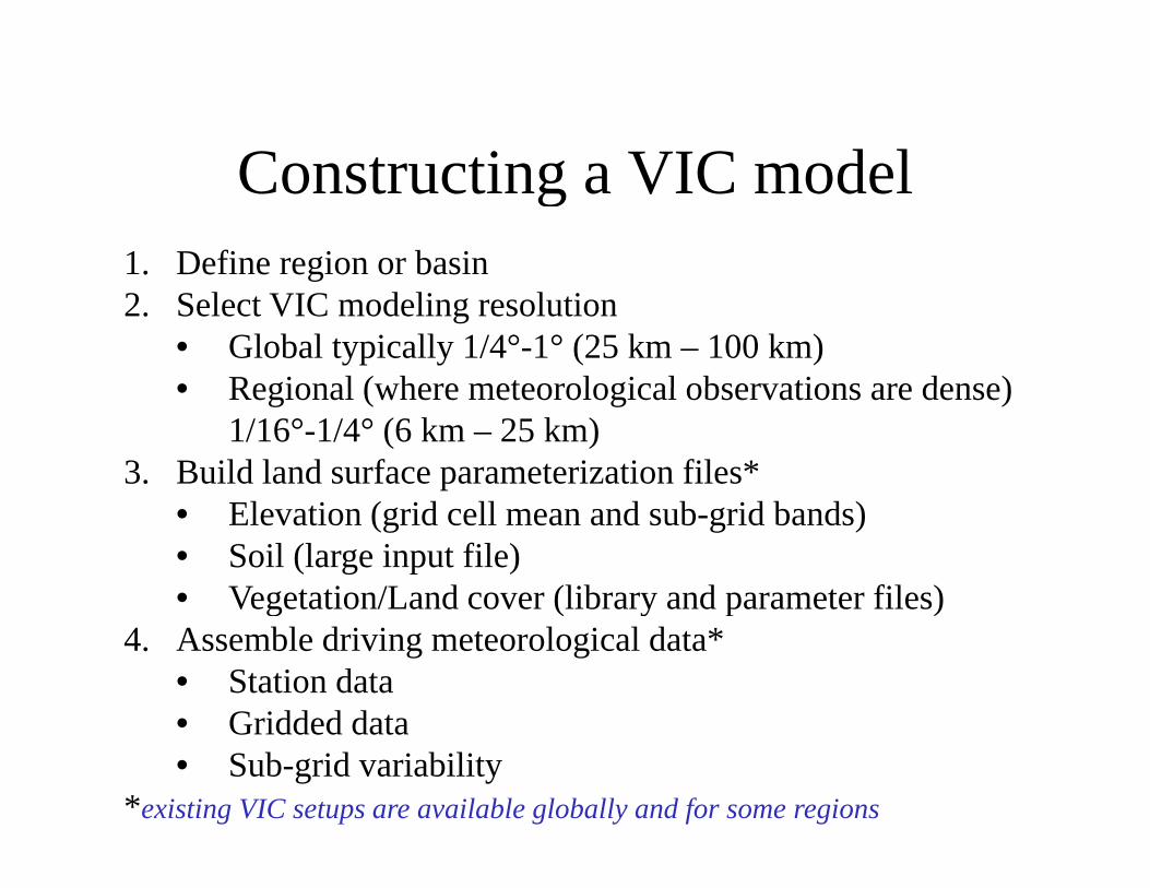
Constr cting a VIC modelConstructing a VIC model1. Define region or basing2. Select VIC modeling resolution

• Global typically 1/4°-1° (25 km – 100 km)• Regional (where meteorological observations are dense)• Regional (where meteorological observations are dense)

1/16°-1/4° (6 km – 25 km)3. Build land surface parameterization files*

• Elevation (grid cell mean and sub-grid bands)• Soil (large input file)• Vegetation/Land cover (library and parameter files)g ( y p )

4. Assemble driving meteorological data*• Station data• Gridded data• Gridded data• Sub-grid variability

*existing VIC setups are available globally and for some regions

Running VIC in a nutshellMeteorologicalMeteorologicalForcing Files

VICS b d Fil Fluxes @ grid cellVICModel

Snowbands File

Vegetation File

Fluxes @ grid cell

RoutingFraction File

Vegetation File

Global parameterfile

RoutingModel

Flow Direct.File

Xmask file

Qobserved

fileRout Inputfile

Qsimulated

Q

time

Slide courtesy of E. de Maria

Defining modeling domain: Basing g

Select basin from existing data

or

Define rectangle of interestinterest

Select VIC modeling resolutionNote: VIC doesn’t know about basin boundaries – you can model a larger area thanmodel a larger area than needed, as long as it contains your basin

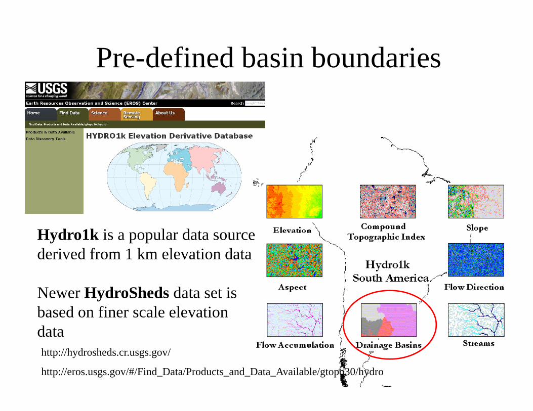
Pre-defined basin boundaries

H d 1k i l d tHydro1k is a popular data source derived from 1 km elevation data

Newer HydroSheds data set is based on finer scale elevation datahttp://hydrosheds.cr.usgs.gov/

http://eros.usgs.gov/#/Find_Data/Products_and_Data_Available/gtopo30/hydro

data

Digital Elevation ModelsDigital Elevation Models• Hydro1k: equal area projection, 1 km resolution• Gtopo30 or SRTM30: geographic projection, 30

arc-seconds (~ 1 km)http://edc.usgs.gov/products/elevation/gtopo30/gtopo30.htmlhttp://topex.ucsd.edu/WWW_html/srtm30_plus.html

Newer, higher resolution elevation data

•Derived from elevation data of the Shuttle Radar Topography Mission (SRTM) t 3 d l ti ( 90 )at 3 arc-second resolution (~90m)

•Stream networks, watershed boundaries, flow direction and accumulation •http://hydrosheds.cr.usgs.gov

Extract Elevation Information forExtract Elevation Information for Basin/Region

• Extract/clip elevation data to basin or region• Project to geographic (if necessary)j g g p ( y)• Aggregate it to the VIC modeling resolution• Retain fine-scale elevation data for elevation band

definition (sub-grid scale detail)

Elevation derivatives (availableElevation derivatives (available from Hydro1k and HydroSheds)

• From elevation data source, it may also be useful to download, for the identical domain:– Basin boundaries– Flow directions

l l i– Flow accumulations– Rivers

Whil th b d i d f l ti i• While these can be derived from elevation using GIS, obtaining from the same source guarantees consistencyconsistency

• These can also be used in later processing steps.

Describing Land Cover

• Two files describe this in VIC1. Vegetation library file: describes1. Vegetation library file: describes

hydrologically important characteristics of different land cover types

2. Vegetation parameter file: contains the spatial variability of land cover

Land Cover ClassificationLand Cover Classification• U. Maryland AVHRR, 1 km global product

http://glcf miacs md ed /data/landco er/– http://glcf.umiacs.umd.edu/data/landcover/

• IGBP global product– http://landcover.usgs.gov/globallandcover.php

Sources of land cover parametersp

Literature•Many potential sources•Use functions to derive from NDVINDVI

http://ldas gsfc nasa gov/nldas/web/web veg table html

Assembled databases

http://ldas.gsfc.nasa.gov/nldas/web/web.veg.table.html

•e.g., LDAS (http://ldas.gsfc.nasa.gov)•Available in gridded formatAvailable in gridded format at 1/4° spatial resolution globally

Vegetation-related parametersVegetation type Albedo Rmin

(sm-1)LAI Rough

(m)Displacement（m）

1 Evergreen needleleaf forest 0.12 250 3.4-4.4 1.476 8.04

2 Evergreen broadleaf forest 0.12 250 3.4-4.4 1.476 8.04

3 Deciduous needleleaf forest

0.18 150 1.52-5 1.23 6.7forest

4 Deciduous broadleaf forest 0.18 150 1.52-5 1.23 6.7

5 Mixed forest 0.18 200 1.52-5 1.23 6.7

6 Woodland 0 18 200 1 52-5 1 23 6 76 Woodland 0.18 200 1.52-5 1.23 6.7

7 Wooded grasslands 0.19 125 2.2-3.85 0.495 1

8 Closed shrublands 0.19 135 2.2-3.85 0.495 1

9 Open shrublands 0.19 135 2.2-3.85 0.495 1

10 Grasslands 0.2 120 2.2-3.85 0.0738 0.402

11 Crop land (corn) 0.1 120 0.02-5 0.006 1.005

Index vegetation characteristics to classification.

Vegetation library file formatVegetation library file format

• One 58-column file used for all VIC model grid cellsmodel grid cells

Sample vegetation library filerelates land cover class to vegetation characteristicsrelates land cover class to vegetation characteristics

Vegetation parameter file

• One large file describing land cover contents of each grid cell

• Format described on VIC b iweb site

• Can include “global LAI” i f ti d ibiinformation, describing monthly LAI for each vegetation type at each gridvegetation type at each grid cell

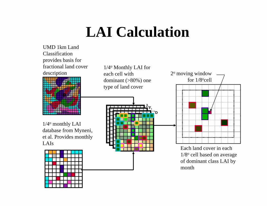
LAI CalculationUMD 1km Land Classification provides basis for fractional land cover description 2o moving window

for 1/8ocell

1/4o Monthly LAI for each cell with dominant (>80%) one type of land cover

J, F, .., D

1/4o monthly LAI database from Myneni, et al. Provides monthly LAILAIs

Each land cover in each 1/8o cell based on average of dominant class LAI by monthmonth

Sample lines from vegetation parameter file

Soil Information• UNESCO/FAO global soil maps

– http://www.fao.org/geonetworkhttp://www.fao.org/geonetwork– Available as 5 arc-min grid (~8km resolution)

• IGBP-DIS data• http://daac ornl gov/SOILS/igbp html• http://daac.ornl.gov/SOILS/igbp.html• Includes derived data products

Using LDAS data

• As with vegetation data, LDAS has pre-processed soil data for the US and globally

• http://ldas.gsfc.nasa.gov/gldas/GLDASsoils.php

Translating soil composition/texture to hydraulic properties

Constructing the soil fileConstructing the soil file

• This is the principal input file: – connects cell location to cell number– defines which cells to run

• Number of columns depends on number of soil layers.

• For 3 soil layers, 53 or 54 columns is y ,typical.

• Some columns only used in energy balance mode, may contain any , y yarbitrary value if not used

• Main calibration parameters are in this file

• One approach outlined at http://www.hydro.washington.edu/~nathalie/VIC_FILES/VIC_SoilVeg_processing.html

Sample Soil File

• 1 column per parameter, 1 row per grid cell

Meteorological Data

• Individual meteorological data file for each grid cellg

• Obtained by:Interpolating observed data onto VIC grid– Interpolating observed data onto VIC grid

– Using existing gridded data sourcesCombining existing gridded data with– Combining existing gridded data with additional information from observations

Meteorological input is flexibleMeteorological input is flexible

Daily VIC Model Forcing Data - Typical

Forcing Data based on observations:• Precipitation (mm)p• Daily maximum temperature (°C)• Daily minimum temperature (°C)• Wind speed (m/s) (from reanalysis)Wind speed (m/s) (from reanalysis)Other (less well observed variables) estimated using

parameterizations (Kimball et al., 1997, Thornton and Running, 1999):

Humidity (Vapor Pressure): uses MTCLIM - Tdewestimated from Tmin (with aridity index based on Pannualand Rsolar)

D d S l R di tiDownward Solar Radiation: transmissivity estimated from Tdew, Tmax – Tmin

Downward Longwave Radiation: estimated from T , humidity, atm. transmissivityTaverage, humidity, atm. transmissivity

Interpolating Temperature and Precipitation DataPrecipitation Data

Avg. Station density:Area Km2/station

Within the U.S.:•Precipitation adjusted for time-of-observation

U.S. 700-1000

Canada 2500

•Precipitation re-scaled to match PRISM mean for 1961-90

Mexico 6000

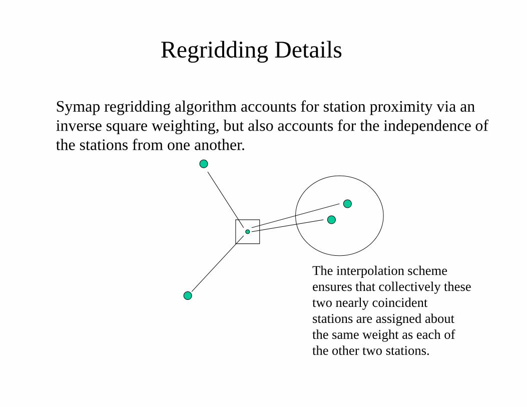
Regridding Details

Symap regridding algorithm accounts for station proximity via an inverse square weighting but also accounts for the independence ofinverse square weighting, but also accounts for the independence of the stations from one another.

The interpolation scheme ensures that collectively these two nearly coincident stations are assigned about th i ht h fthe same weight as each of the other two stations.

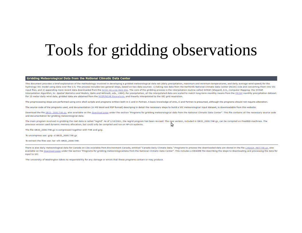
Tools for gridding observations

Global meteorology

Densities lower for much of globeDaily records from 17 000 stations butDaily records from ~17,000 stations, but important areas lack coverageGridded data relies on a variety of sources

CPC/NCEP/NOAAMaurer et al., 2009

Final meteorological filesgEach grid cell has its own met data file.Fil b f f fil fi l lFile name must be of format <filename_prefix>_<lat>_<lon>

Contents are user definedContents are user-defined

Sub-grid topography:l i ( ) b delevation (snow) bands

Especially important in snow-dominated areas

Next Steps to run VIC

1. Prepare VIC Global Control File• Identifies soil, vegetation, meteorology files

Gi l i f fil• Gives location for output files• Sets modes for VIC operation• Supplies global parameter valuespp g p• Supplies meteorological input file format• Selects variables to output

2 Run VIC2. Run VIC3. Route runoff and baseflow to a stream point4. Compare to observed streamflow and calibrate VIC

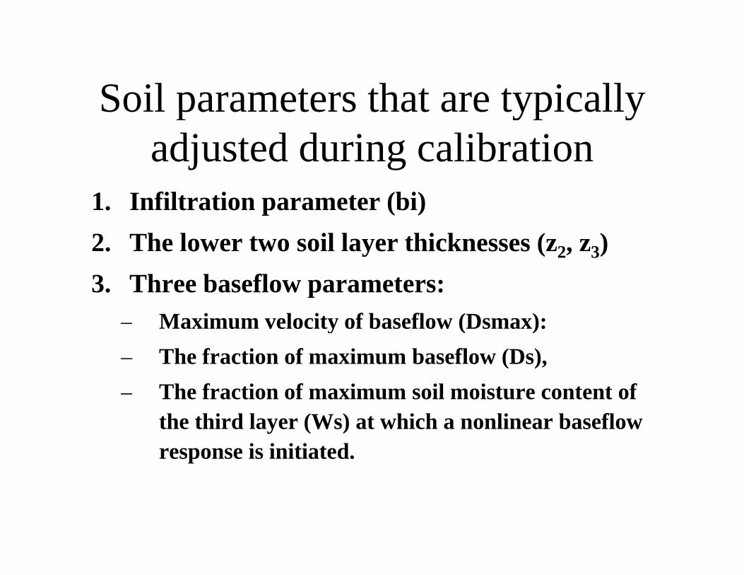
Soil parameters that are typicallySoil parameters that are typically adjusted during calibration

1. Infiltration parameter (bi)2. The lower two soil layer thicknesses (z2, z3). e owe wo so ye c esses ( 2, 3)3. Three baseflow parameters:

– Maximum velocity of baseflow (Dsmax):Maximum velocity of baseflow (Dsmax):– The fraction of maximum baseflow (Ds),– The fraction of maximum soil moisture content ofThe fraction of maximum soil moisture content of

the third layer (Ws) at which a nonlinear baseflow response is initiated.

Other parameters that can beOther parameters that can be included in calibration

• T max for snow• T min for rainT min for rain• Precipitation scaling

O hi ff• Orographic effects