INTRODUCTION

Studies of alluvial landscapes often reveal a wide range of soil forms distributed in complex

patterns. in Australia, these phenomena have been explained largely in terms of cycles of fluvial

erosion and deposition during the Quaternary. Soil differences within alluvial landscapes of

eastern coastal streams have been interpreted as being essentially the result of progressive soil

development with time (Walker and Coventry 1976). However, these and other pedogenctic stu-

dies have been restricted to soils developed from coarse to medium textured parent alluvium. In

contrast, comparatively little has been published on explaining soil distribution patterns and pro-

gressive soil development on clay-rich alluvium.

Clayey alluvial plains occur extensively in the Lockyer Valley of south-east Queensland

where cracking clays (Vertisols) are widely distributed. Despite these soils being among the most

highly productive in Queensland, little is known in detail about their nature and distribution. In

order to explain features of the Lockyer Valley alluvial soil landscape, an interdisciplinary study

was established incorporating pedology, geomorphology and statistics.

The alluvia together with selected upslope sites within the Tenthill Creek catchment and

part of Lockyer Creek were selected for study (see Fig. 4.1). This area was chosen because the

Tenthill Creek tributary has the largest catchment area in the Lockyer Valley and is the main

source of alluvia for Lockyer Creek within the confines of the study area.

The investigation had four objectives:

(i) To investigate the origin of parent alluvium using the clay and fine sand mineralogy of

upslope source materials and soils of the alluvial landscape.

(ii) To survey and map the soils of the alluvial landscape in order to describe the range of soils

found, and to show interrelationships and spatial distributions which might assist in inter-

preting their genesis.

(iii) To assess by statistical means some aspects of the morphological variability of soils within

an alluvial plain landscape of low relief.

-2-

(iv) To develop a soil-geomorphic framework which explains the patterns of soils found on the

alluvial landscape in terms of soil stratigraphic units associated with episodes of valley

development.

- 3 -

REVIEW OF LITERATURE

Many studies of alluvial soil landscapes have shown them to be the result of complex histories of

fluvial erosion and deposition. The literature review is aimed at gaining an understanding of the

fundamental alluvial processes that have led to the development of particular soils and landforms.

It is also aimed at reviewing the geomorphic factors responsible for the development of alluvial

soil landscapes of eastern Australia in general. Finally, some of the methods used by other workers

to investigate alluvial soil landscapes are described and evaluated.

1. DEVELOPMENT OF ALLUVIAL LANDSCAPES

1.1. Introduction

To understand and improve the prediction of soil distribution in an alluvial landscape, a

knowledge of the processes responsible for the composition and shape of alluvial landforms is

necessary. Deposited alluvium represents a sediment sink in which water eroded and sorted sedi-

ments accumulate, are reworked, or undergo biogenic or pedogenic processes for extended

timespans. Each alluvial deposit within a fluvial system may be associated with sediment of

different composition, and therefore when acting as soil parent materials, the properties of soils

which form on them may differ considerably.

1.2. Nature of deposited alluvium

Alluvium is unconsolidated sediment of relatively recent geological age that was deposited by

water (Bloom 1978). Alluvium covers the bedrock floors of river valleys and builds up fans or del-

tas where stream competence* abruptly decreases. It may also occur as a ribbon-like deposit on

* Competence - a measure of the streams ability to transport a certain maximum grain size of sediment (Bloom 1978).

upland surfaces, marking the former course of a now-diverted stream, or less clearly delineated as

isolated remnants following stream truncation.

- 4 -

Weathered rocks are carried by rivers in three forms (Bloom 1978). The compounds in solu-

tion are the dissolved load. The solid matter is either fine grained particles in suspension

(suspended load) or coarser grained particles that slide, roll and bounce along the stream bed

(bed load). The alluvium is then deposited, either by vertical accretion consisting largely of

suspended load materials, or by lateral accretion of bed load.

Quaternary tectonism and climatic fluctuations have made alluvium a complex material to

interpret. The distinction between alluvium actively "in transit" and "relict" is often difficult.

The thickness of modern alluvium can be defined by stream capacity t and the flood scour

Capacity - theoretical maximum amount of sediment that a stream can transport (Bloom 1978).

depth of the modern channel, and its maximum grain size by the flood-stage competence of the

modern stream (Bloom 1978). Anything deeper or coarser is "relict" alluvium. Alluvium on ter-

races not currently flooded can also be considered to be relict.

Coarse alluvium decreases in mean grain size downstream by sorting and abrasion (Bloom

1978). Size sorting by progressive loss of competence downstream is the major cause of decreasing

grain size in alluvium. There is, however, a complex interplay between bed roughness, velocity,

slope and grain size. In addition bed load aggregates do not readily survive fluvial transport

beyond their slopes of origin because of fragmentation due to grain collisions in water flow associ-

ated with channels. (Moss 1972).

River channels may be classified according to the nature of their load and their stream bed

characteristics. Schumm (1977) separated suspended-, mixed- and bedload streams on the nature

of their load. Pickup (198 ,1) defined source reaches, where the channel is in contact with bedrock;

armoured reaches, where the bed is protected by a veneer of coarse bedload material; and mobile

zones, where bed material is line enough to be transported by large flows and sink zones, where

backwater effects from larger streams or coastal systems may cause deposition of fines on the bed.

This classification has some compatibility with traditional channel definitions of bedrock channels

eroded into the regional rock and alluvial channels, cut into the alluvium. Bedrock channels are

- 5 -

likely to be more irregular than alluvial channels (Bloom 1978).

1.3. Behaviour of river systems

1.3.1. Introduction

An understanding of the behaviour of rivers can give an insight into the processes that produce

various alluvial sedimentary sequences. Observations of channel morphology are useful for inter-

preting the past erosion/depositional behaviour of streams and also the composition of the alluvial

load.

1.3.2. River competence

River competence, the relationship between mean velocity in a river and the size of particle that

can be eroded or transported by it, is illustrated in Fig. 1.1 (Hjulstroem 1935, 1939, Sundborg

1956). These curves were derived from flume experiments on well-sorted sediments. When coarse

and fine sands are mixed, the fine particles fill spaces between the coarse ones and are thereby pro-

tected, and also help prevent the coarse grains from moving (Blatt et al. 1972).

Estimation of river competence cannot be accurately derived from these curves using aver-

age stream velocity, because this is not the velocity at the bank or bed of the stream, where much

of the erosion and transport occur. A point on the graphed line between the transport and sedi-

mentation fields represents the mean velocity in a stream at least 1 m deep that will provide

sufficient turbulence to keep a particle of given size from settling out of suspension. The upper

curve ("Iljulstroem's curve") is actually a field of values for the velocity necessary to initially

entrain particles. The position of this curve has been estimated by Sundborg (1956) to occur at

higher velocities.

-6-

Transportation

Sedimentation

001 002 .005 01 02 .05

2 5 1.0 2.0 5 0 10 20 50 100 200 500

Particle size (mm)

Fig. 1.1. Relation of mean current velocity of water at least 1 m deep to the size of mineralgrains that can be eroded from a bed of similar-sized grains and transported by the current.Dashed lines on upper curve are revisions proposed by Sundborg (1956).

The quantity of suspended sediment transported by a stream at any one time is a function

of sediment supply rather than the transporting power of the stream (Douglas 1977). In contrast,

bedload transport is more closely related to channel hydraulics. For pebbles, cobbles and bould-

ers, the erosion threshold is only slightly greater than the transportation velocity, because they

barely rise from the bottom as the bounce or roll as bedload. Actually, large stones on the bed of

a stream are overturned or rolled by mean velocities less than those indicated by the Hjulstroein

curve (Bloom 1978). The exact relationship between eroding velocities and large particle sizes has

yet to be established (Novak 1973). Probably 95 percent of the total work done by stream tran-

sport is ascribed to the few percent of the load that have the coarsest grain sizes (Bagnold 1968).

Silt and clay sizes are kept in suspension by very slight currents, but the velocities necessary to

erode a consolidated clay bank are comparable to those that move pebbles and cobbles (Fig. 1.1).

A muddy river bed may resist stream flow and induce friction as much as a gravel bed on

account of cohesion between particles. Channel roughness is an important but complex parameter

7

of fluvial process that is related not only to velocity and grain size but also to a depth parameter,

bedform (rippled, smooth, etc.), and channelslope (Bloom 1978).

In alluvial channels, the downstream changes in bed roughness and the increased width and

depth of the channel provide less turbulence and therefore less competence to move coarse sedi-

ment.

1.3.3. River capacity

When load is measured it is usually the suspended component that is measured. Leopold and Mad-

dock (1953) found that suspended load is determined by the parameters of discharge, width,

depth, velocity, slope, bed roughness and grain size of the load. Measurements of channel shape

and suspended-sediment load by these workers confirm that streams move most of their loads dur-

ing times of higher than average discharge. As the water rises during a flood, alluvial channels

were found to initially aggrade their bed. Leopold and Maddock (1953) believed that the aggra,da-

tion resulted from a sudden influx of new sediment from the uplands and the decreased roughness

effect of the more dense water sediment mixture. During the peak flood discharge, the channel

may be scoured even deeper than the preflood level and then aggrade again during the declining

discharge late in the flood. Thus competence is not simply correlated with velocity. At a given

velocity during increasing discharge, bed aggradation occurs, but when the same velocity is

reached after the flood crest has passed, the bed may be eroded (Leopold and Maddock, 1953).

Differences are considered to be due to hydraulic factors changing in response to changing load.

The nature of the dominant discharge event that occurs within a channel can be qualita-

tively assessed by examining channel form and allocating one of Tricart's (1960) four channel

types:

(i) Base flow channel: occupies the channel floor between vegetated banks and carries the lowest

flows, which often wind through the gravels or sands of minor channels.

(ii) Minor channel: steep almost continuous banks which rise from the channel floor. Flows in

the minor channel are sufficiently frequent to prevent growth of vegetation. The upper part

-8

of the banks, however, have grass cover with shrubs or rapidly growing trees.

(iii) Periodic major channel: is occupied by floods occurring at least once per year. Only plants

that can withstand submergence grow.

(iv) Exceptional major channel: is occasionally filled by major floods. Floods are so infrequent in

this channel that vegetation differs little from interfluve areas outside the flood channel.

1.3.4. Channel pattern and solid load

In the alluvial channel there is a constant exchange taking place between the channel bed and

load. Even though the channel is primarily shaped during high discharge, lesser discharges have

velocities of certain competence which selectively move grains up to a certain size limit. The com-

plex readjustment between discharge, grain size of the load (and bed), velocity, and the amount of

load results in the formation of a variety of channel patterns (Bloom 1978).

The channel pattern of a river is usually considered to be straight, meandering or braided.

However, an intermediate pattern between straight, and meandering has been called sinuous. In

addition Schumm (1968) proposed the term anastoinosing for braided patterns where islands divid-

ing the channels are stable. Morisawa (1985) has summarised the properties and behaviour of these

patterns as shown in Table 1.1 and Fig. 1.2.

Rivers that carry primarily sand and gravel as bed load develop wide, shallow alluvial chan-

nels and are often braided Braided channels most commonly occur in the steep upper reaches of

a river, where transporting power is high and it is thought that the braiding process tends to dissi-

pate this power by spreading the flow over a number of channels (Henderson 1966).

- 9 -

Table 1.1. Classification of river patterns (Morisawa (1985), partly based on Schumm (1972)and Miall (1977)).

Type Morphology Sinuosity* Load-type Width/ Erosive behaviour Depositonal behaviourindex depth

ratio

Straight Single Channel with <1.05 Suspension- <40 Minor channel Skew shoals

pools and riffles, mixed or widening andmeandering talweg bedload incision

Sinuous Single channel, pools >1.05 Mixed <40 Increased channel Skew shoals

and riffles <1.5 widening and

meandering talweg incision

Meandering Single channels (may > 1.5 Suspension- <40 Channel incision Point bar formation

be inner point bar or mixed meander

channels load widening

Braided

Two or more channels >1.3 Bedload >40 Channel widening Channel aggradation,

with bars and small mid-channel bar

islands formation

Anastomosing Two or more channels >2.0

Suspension <10 Slow meander Slow bank accretion

with large, stable islands load widening

* Sinuosity index - ratio of channel length to clown-valley distance

Fig. 1.2. Channel patterns as described in Table 1.1. Adapted from Miall (1977).

Where bed load is carried near the bottom of the braided stream, stream velocity is lower,

whereas faster moving upper water can erode banks made of grain sizes similar to those already in

- 10 -

transport as bed load. In addition, sand and gravel are noncohesive, and banks of coarse alluvium

collapse readily, to be spread out on the flat, shallow bed. (Bloom 1978). In times of low

discharge, a braided river may disappear entirely as the water sinks into the loose sands and grav-

els, and flows below the surface.

Rivers that carry mostly silt and clay as suspended load develop deeper, narrower channels

with a catenary or trapezoid cross section. This shape minimises surface area and friction, and

thus provides for maximum transport of suspended load, which is carried by internal turbulence,

rather than bed shear. The steep banks can be undercut, but the cohesive strength of consoli-

dated silt and clay resists bank erosion (Bloom 1978).

Schumm (1960a, 1960b) established that the width-to-depth ratio of rivers on the Great

Plains of North America is inversely proportional to the percentage of fine-grained sediment in the

banks, and therefore also in the load. The braided habit of such rivers is partly an internal adjust-

ment among semi-dependent variables of width, depth and sediment grain size, and partly a

response to the independent variables of discharge and load.

Meandering channels usually occur on lower gentler slopes towards the river mouth, and the

river flows in one well defined channel. Meander systems tend to extend and perpetuate them-

selves by the scouring action of the flow on the outside of each curve. Any slight initial departure

from the straight channel form will lead to the eventual development of a meander pattern

(Henderson 1966). In a river with erosion resistant banks, downcutting would predominate, and

the meanders become incised. If downcutting and lateral extension occur together, the meanders

increase in sinuosity whilst being incised to produce an ingrown meander.

The meandering habit of many rivers, especially those that flow on fine-grained alluvium in

humid regions, is also related to the width-depth ratio of the channel and sediment grain size. As

the suspended-sediment load increases in proportion to bed load, the channel narrows and

deepens. By these interrelated adjustments, more of the energy of the stream is expended against

the banks and less against the deep bottom. The sinuousity of the channel increases, and

meanders form (Bloom 1978).

The wavelength of meanders shows a close correlation with mean annual discharge more so0 1

than with bankfull discharges (Gerrard 1981). Thus meander form appears to be determined

largely by the average flow of the river. Some meanders show a wavelength far too large for their

present discharge, suggesting periods of greater discharge in the past.

Along meandering downstream channels, alternating pools and ri

tend to occur. A range of particle sizes is necessary for this development, with uniform sand or

silt having little tendency to form pools and riffles (Douglas 1977). According to Yang (1971), pool

and riffle formation is the vertical adjustment, in contrast to meandering lateral adjustment of a

river, to minimise the time rate of potential energy expenditure per unit mass of water along its

course of flow.

In flume experiments, Schumm and Khan (1972) attempted to produce meandering channels

by varying slope, discharge, and sediment loads. They were able to produce channels with alter-

nating bars and pools so that the thalweg fluctuated vertically, but the channel banks remained

essentially straight until the stream abruptly developed midchannel bars and became braided.

The sediment in the flume was poorly sorted sand. A truly meandering channel could not he

formed until 3 percent by weight of kaolinite clay was mixed into the water. The clay coated and

stabilised the banks and bars and allowed the thalweg to deepen and expose the stabilised sand-

bars on alternating sides of the channel True meanders formed. The experiment illustrates well

the action of alluvial grain size as a factor in the hydraulic geometry of rivers.

Transitional forms are rare between wide, shallow channels with a braided habit and nar-

rower, deeper channels that meander. Some reaches of rivers have changed historically from

braiding to meandering to braiding again (Schumm 1969), but the changes are abrupt. Perhaps

the lack of intermediate forms is related to the fact that the minimum threshold of sediment ero-

sion on I-Uulstroem's curve (Fig. 1.1) is in the medium sand size. If the alluvium is noncohesive

sand or coarser sediment, rising velocity drags it as bed load, and a wide, shallow braided channel

develops. If the alluvium is cohesive, an equivalent velocity increase may erode it, but it is tran-

sported as suspended load in a deep, meandering channel.

flies (topographic highs)

- 12 -

However, Lewin (1978) suggests that the simple division of channels into between two and

four exclusive types (meandering and braided, with the possible addition of straight or anastomos-

ing) is seldom satisfactory in practice. Braids can meander and meanders locally braid; straightish

channels may consist of a single stream at formative high flows, but split into many low flow

channels; and meanders may have such complexity that associated floodplain forms cannot be

predicted without a very detailed appreciation of river activity.

3 4 6 75 1 2

TRANSPORTATIONAL MIUSLOPE(frequently occurring

angles 26°-35')0 INDICATES MOVEMENT IN

A DOWNVALLEY DIRECTION

ARROWS INDICATE DIRECTION AND

RELATIVE INTENSITY OF MOVEMENT OF

WEATHERED ROCK & SOIL MATERIALS

BY DOMINANT GEOMORPHIC PROCESSES

COLLUVIAL

FOOTSLOPE ALLUVIAL404, TOESLOPE6 CHANNEL

SOS(° 0, , 1 0

riavtOF

0°-4°

, a( ,-.0 :'-' iLai _JI -- LI CC _J 0.. •V -. ...,r, L.-!-.- .`i 6

• ,

IIWX X .S.7- t*

W“J

CC L I-

1N

'6 f., & ''T - 0 ,

.) artw3

wJ c.• 0, La•.

.2d•-• ,t, • _.J •-•

'&j .6 un vl

›-U — r.

__I O.''' ''' i . _ 41 .1 Lt.-1 __I •

..

..W , .`” T

d i,

c•-■.2 X X. 0 co •— O C,Ncai La CD

0 ,• X•-• D I_•- X .;••-FCC N

O N •:(

>- .-/ Lai D, N N 3

8PREDOMINANT CONTEMPORARY GEOMORPHIC PROCESSES

CHANNEL

eco9

.71

• .X (7,1LA_ CD V,

• C, ak

9

- 13 -

1.4. Types of alluvial landforms

1.4.1. Introduction

The geomorphic processes responsible for fluvial depositional landscapes produce a variety of land-

forms, usually differing from each other in their sediment composition. .Dalrymple et al. (1968)

developed a hypothetical nine-unit land surface model, which relates dominant geomorphic

processes to nine specific land form elements (Fig. 1.3). The low relief land units 6 to 9 are the

most common landform elements of fluvial depositional landscapes.

1NTERFLUVE

1 SEEPAGE SLOPE

2

0°-1° 2°-4°

Modal slope angles4 FALL FACE

(minimum angle 45'

normally over 65°)

Fig. 1.3. Diagrammatic representation of a hypothetical nine-unit land surface model (after Dal-rymple et al. 1968).

CONVEX

CREEP

SLOPE

3

- 14 -

Fluvial depositional landscapes are fashioned from unconsolidated sediments weathered from

bedrock in one area and transported by water to another area. Thus not only are they much

younger than the underlying bedrock, they are also unrelated to it. Depositional landforms may

be distinguished from surrounding in situ landforms by differences in shape, landscape position,

vegetation, microrelief, coarse fragment composition and abundance of surface deposits, and soil

profile properties. In some regions, e.g. the Riverina Plains of Australia, fluvial deposition may be

interlayered or intermixed with material of aeolian origin (Butler 1956), which may be difficult to

separate.

The more common fluvial despositional landforms are illustrated in Fig. 1.4 and genetically

characterised in Table 1.2.

Fig. 1.4. Typical associations of valley sediments. A-Alluvial fan; B-Backland; BS-Backswamp;C-Colluvium; F-Channel fill; L-Lag deposit; LA-Lateral accretion; N-Natural levee; P-Point bar;S-Splay; T-Transitory bar; VA-Vertical accretion; after Vanoni (1971).

- 15 -

Table 1.2. Genetic classification of valley sediments (Vanoni 1071).

Place of deposition Name Characteristics

Channel Transitory channel deposits Primarily bed load temporarily at rest; part

may be preserved in more durable channel fills

or lateral accretions.

Lag deposits Segregations of larger of heavier particles, more

persistent than transitory channel deposits, and

including heavy mineral placers.

Channel fills Accumulations in abandoned or aggrading

channel segments; ranging from relatively

coarse bed load to fine-grained oxbow lake

deposits.

Channel margin Lateral accretion deposits Point and marginal bars that may be preservedby channel shifting and added to overbank

floodplain by vertical accretion deposits at top.

Overbank flood plain Vertical accretion deposits Fine-grained sediment deposited from suspend-

ed load of overbank flood water; including na-

tural levee and backland (backswamp) deposits.

Splays Local accumulations of bed-load materials,

spread from channels onto adjacent flood

plains.

Valley margin Colluvium Deposits derived chiefly from unconcentrated

slope wash and soil creep on adjacent valley

sides.

Mass movement deposits Earth flow, debris avalanche and landslide

deposits commonly intermix with marginal col-

luvium; mud flows usually follow channels but

also spill overbank

In their investigation of the various deposits of the Indus Valley, Holmes and Western (1960)

found a range of characteristic texture profiles associated with different landforms (Table 1.3).

Table 1.3 illustrates the potential complexity that can be associated within even one landform

type of a specific river system. Thus soils of similar age found on such landforms may show con-

siderable diversity of profile form.

- 16 -

Table 1.3. Characteristic textures of landform types in the Indus Valley(Holmes and Western 1909).

Landform association Characteristic texture in order of occurrence

bank levee deposits

spillway levee deposits

flood levee deposits

dominantly coarse sand and loamy sand

mixture of sands and loams; sometimes complex; dominantly coarse sand andloamy sand; silts and clays overlie sands and loarns at depths <50 cm;

almost entirely silts and loams; clays probably dominant; silts and clay overliesands and loams at depths <50 cm; upper horizons dominated by clay.

almost entirely silts and clays; dominantly coarse sand and heavy sand: sandsand loams overlie silts and clays at depths >50 cm; complex but basiclly sandsand loams.

mixture of sands and loarns, sometimes complex; sands and loarns overlie siltsand clays at depths >50 cm

dominantly coarse sand and loamy sand; mixture of sands and loamy, sometimescomplex sands and loarns overlie silts and clays at any depth.

high bar deposits

low bar deposits andchannel scar deposits

channel infill deposits

anthropic levee deposits mixture of sands and loarns; sands and loams overlie silts and clays at any depth.

shallow cover floodplain upper horizons dominated by clay; silts and clays ovrlie sands and loarns atdepths >100 cm; almost entirely silts and clays.

backsw amp deposits silts or clays.

Details on the nature and development of the more common alluvial landforms are outlined

in the following sections.

1.4.2. Alluvial fans

An alluvial fan is a segment of a low cone with its apex at the mouth of a gorge or drainage line

(Bloom 1978). It usually forms where a high gradient tributary abruptly enters onto a floodplain

of a trunk stream or valley. If the slope of the terrain is steep, as where minor streams descend

from upland areas, the feature is called an alluvial cone (Thornbury 1969). Adjoining fans fre-

quently coalesce to form an apron of talus in front of a dissected scarp. The processes responsible

for fan formation are described in most geomorphological texts (e.g. Fairbridge 1968, Thornbury

1969, Bloom 1978).

- 17 -

Fans are normally built of bed load alluvium especially gravel (Fig. 1.5). Stratification of the

fan may be obvious or it may contain many cut and fill structures of buried channels. Branching

radiating distributary channels are most often braided rather than meandering. The permeable

character of fan alluvium allows considerable infiltration, so that desert fans may contain mudflow

deposits recording the progressive loss of water until the suspended load becomes too thick to flow

as a muddy stream.

Fans are aggradational or built-up forms. One radial channel may carry most of the

discharge for a time until it becomes filled with sediment, and the stream abruptly shifts to form a

new channel. This process ensures a relatively uniform slope development along all radii and

results in a smooth conical form. However, a complex soil distribution may also be found as a

result of short distance variability of sediments and differences in age of deposits.

The building of fans occurs largely during flood times, when large volumes of water and

entrained alluvium debouch onto them. Much of the time stream channels across fans are dry, or,

if permanent streams, much of the water sinks into the course alluvium near the fan apex. At the

toe of the fan, abandoned stream channels of the master stream terrace may be filled for some dis-

tance by fan material.

Some underfit t trunk streams have low gradients and cannot transport the coarse alluvium

Underfit stream: a stream that appears too small to have eroded the valley in which it flows (Amer. Geol. Inst. 1974).

delivered by valley side tributaries, and the master stream is pushed laterally from one valley wall

to the other by fans. Some fans may even block a trunk stream and cause a lake.

Large areas of semi arid grasslands, such as Russian steppes, American prairies or pampas,

and the South African veld, are constructional surfaces of huge coalescing piedmont § alluvial fans

(Bloom 1978).

Piedmont: lying or formed at the base of mountains (Amer. Geol. Inst. 1974).

Middle fan.Buried toe

1

Toe.

4I) Idealized cross section of a fan.

A) Initial stage.

,0 9tt3° c'''E`5` • '....,r°075?-. 0:° 'Ns" '00C, o 0° -0 a

B) Initial fan buried by later fan.

(R. Co4,

Q

0o t̂,c) 0.0.7, 013 0 0 0,0 c, 0 0 „, 0°.`CS ° '0,01;;I° ° e I.) CI 0° 0 0 o

C) Later stage showing buried toe sediments.

Fonh ea d.

Coarse, porous tanhead sediments.Mixed middle fan. sediments.Fine toe sediments.Terrace gravels.

7VENNAPID

-18-

Fig. 1.5. Stages in growth of a fan and development of a sole layer (after McCraw 1968).

The dominant landform associated with intermontane deserts is the alluvial fan (Fig. 1.6).

The smoothly graded washslope of coalescing fans at the mountain front is a pediment in its upper

parts, where the entire thickness of alluvium is in transit, and a bajada is the lower part where the

alluvium has permanently come to rest in the bolson (mountain basin). Where alluvial fans merge

Pediment pass

- 19 -

in a desert basin, a saline lake (playa) may form. Pediments are regarded as confined to the arid

zones or headwater region and are formed by erosion and deposition of streams usually ephemeral

in type. It is covered in a veneer of gravel in transit from higher to lower levels. It simulates the

form of an alluvial fan (Bryan 1922, cited by Bloom 1978). In arid regions pediments are com-

monly made of hard fresh rock where weathering is slight. In other climates however, some

authors believe analogous pediments may be deeply weathered (Oilier 1969). However, although

there are humid landforms of similar shape to pediments, they may not have been formed by the

processes described above (W. T. Ward, personal communication).

Mountain front

Pediment

Fig. 1.0. Typical assemblage of mountainous desert landforms (after Bloom 1978).

Alluvial fans are also a characteristic of tectonically active regions, and most fans occur in

two possible tectonic settings (Bull 1964). In one, uplift of the mountain front exceeds stream

downcutting and the fan head will not be deeply incised by the stream, resulting in deposition

- 20 -

close to the mountain front. In the other, stream downcutting exceeds uplift of the mountain

front and the stream channel becomes entrenched into the fan, causing deposition on the lower

part of the fan.

If the main river is more energetic or fan growth is slow, movement of the main river chan-

nel from one side of the valley to the other may result in cycles of fan building and truncation (W.

T. Ward personal communication). Truncation of a fan by the river channel steepens the gradient

of the fan building stream, which incises deeper into the fan. Subsequent movement of the main

river away from the truncated fan leads to the growth of a new fan in front of the first. The new

fan may eventually grow to envelop the remnant of the earlier one.

At the head of the fan, shallow stream channels develop as may low terraces. These terraces

can disappear in a relatively short distance down the fan. Terraces may represent periods of

standstill between tectonic uplifts (Twidale et al. 1967) or they may result from episodes of fan

building and degradation of the stream channel (Ward 1967). Where the terrace scarp disappears

in the middle of the fan, stream deposits have overtopped earlier ones giving fans an uniform sur-

face.

Alluvial fans may be conveniently divided into three zones: the fanhead, the middle fan,

and the toe (McCraw 1968). The variation in sediments deposited and the nature of fan develop-

ment in each of these zones is illustrated in Fig. 1.5. As successive deposits enlarge the fan, earlier

toe sediments are buried by the coarse deposits, and new toe deposits are laid down further below.

As the fan grows, fine sediments are thus deposited over the underlying surface to form a 6oic

layer (McCraw 1968). Fan sediments deposited during minor floods may not reach the toe and are

preserved as lenses in the body of the fan.

1.4.3. Washplains

Washplains are the characteristic flat plains found in tropical savanna landscapes in association

with steep sided isolated hills and mountains known as inselbergs. Bloom (1978) described the

processes responsible for this landform. During the wet months, wide areas of the plains are

- 21 -

flooded, and some of the hills become islands. High year-round temperatures and heavy seasonal

rainfall, and associated percolation, operating over long periods of geological time, permit chemi-

cal weathering to extend to great depths. With only seasonal runoff, the savanna zone rivers can-

not remove the massive sediment loads furnished by weathering. Rather than entrenching their

valleys, shallow rivers braid or flood across extremely flat washplains. Although the ground sur-

face is a monotonous plain of alluvium and weathered bedrock occurs at depths of up to 100 m,

an irregular weathering front occurs, often associated with a seasonally fluctuating water table.

These plains appear to be the result of both depositional and erosional processes and do not

clearly fit into either a depositional or an erosional landform category.

Various theories have been put forward to explain savanna landscape development. One

theory with a large degree of acceptance is the "double surface of leveling" by Buedel (1957) out-

lined in Fig. 1.7.

This hypothesis can be viewed as an elaboration of the etchplainl l concept.

Etchpiain: is a form of planation surface associated with crystalline shields and other ancient massifs which do nor, dis-play tectonic relief and developed under tropical conditions promoting rapid chemical decomposition of susceptible rocks.

(Thomas 1968).

The concept of etchplain includes both weathered and stripped surfaces, Many authors still

regard these landsurfaces as pediplains, a term which generally describes a series of coalescing ped-

iments (Thornbury 1909). Pediment formations within the weathered materials is believed to

result from the stripping process, and pediments may be formed around residual hills. Under-

standing the evolution of these landscapes is far from complete.

Pediment Pediment

Upper surface: wash plain

Lower surface: basal surface of deep weathering

Recessional or rim inselbergand pediments Shield inselbergs

Lowered wash plain

- 22 -

(a)

Recessional or rim pediments

(b)

Fig. 1.7. Hypothesis of a "double surface of leveling" in a tropical savanna.(a) Wash plain of seasonal flooding is as much as 100 m above the weathering front. Pedimentsfringe the wash plain.(b) Wash plain is lowered by rejuvenation or climatic change. Inselbergs and marginal pedimentsare exhumed or regraded to the lowered wash plains (after Buedel 1957).

1.4.4. Floodplains and terraces

Established river systems usually have their valley floors covered by alluvium, through which a

flow channel is carved. The low relief surface from the banks of the channel to the base of the

valley walls is called the alluvial plain (Speight 1984). If the alluvial plain is characterised by fre-

quently active erosion and aggradation by channelled or over-bank stream flow, it is called a flood

plain (Speight 1984). In flood, part or all of the floodplain becomes the bed of the river (Bloom

1978).

Bankfull flow, dominant channel shaping flow, and the most probable annual flood are

equivalent (Dury et al. 1963). Dury (1967, 1973) has demonstrated that in graded rivers the most

probable annual flood is similar in magnitude to bankfull discharge. Furthermore bankfull

- 23 -

discharge is likely to be reached or exceeded once each year on the average. In rivers where the

most probable annual flood does not exceed its banks, the underfit condition is implied.

The sediment transporting competence and capacity of a river change in flood. Although the

amount of sediment flow in transit is greatly increased along the axis of the permanent channel,

the shallow low velocity sheet of flood water over the adjacent flood plain has little competence;

as velocity is checked, sand, silt and clay may settle out of the floodwaters.

Floodplain landforms are genetically related to specific depositional processes. Not all depo-

sits create landforms however. The lag deposits shown beneath the channel in Fig. 1.4 might well

be relict alluvium.

Floodplains are built by lateral accretion and by vertical accretion. Point bars (Fig. 1.8) are

the most important component of lateral accretion. As a meandering channel migrates across the

floodplain, outerbanks are undercut, eroded and deposited as submerged bars downstream. The

result is a cross-stratified deposit, with subdued relief, which may record many episodes of

meandering channel migration.

In many streams that carry relatively coarse alluvium and lack natural levees, lateral accre-

tion may account for 80-90% of floodplain deposition (Wolman and Leopold 1957).

Catastrophic floods of ephemeral streams may erode and deposit great variability of sedi-

ment facies, or may deposit distinctive sedimentary units during flood peaks. Stear (1985), using

observations of the Laingsburg flood, South Africa as a model, found multistorey deposits to be

the product of a single catastrophic flood event. Thus multistorey deposits do not necessarily

represent numerous separate flood sequences. Interstorey scours could reflect separate erosive

pulses, each with its own set of hydrodynamic variables and resultant sediment profile, accom-

panying various peaks or surges during the same flood episode Fining upward sedimentary

sequences were found to be produced during waning flood stages. Avulsion predominates over sys-

tematic channel migration and, in most cases, high discharge deposits were preserved in preference

to the bedforms deposited in waning flood stages.

suspended loadin over

flow ntiation0 0 ° 0 banksedimentary

differe_. 0

o . . ° ° • • °

° 0 .

•. • • ° ..

'"'N sediments anci Sums

barui s

o •bed load

colloid and so/tires -0-

"9 to fine

- 24 -

During overbank flooding, floodplain deposition is largely by vertical accretion. Deposits

range in particle size from sand to fine clay (Table 1.3), although splays from breached channel

breaks may bring coarser sediment. The abrupt loss of velocity at the edge of the flooded channel

and the abundant sediment supply commonly cause the deposition of more and coarser material

on the natural levees, which grade into finer backswamp deposits. (Fig. 1.8).

1Channel levee near flood

far flood plain,

plain backswamp

Fig. 1.8. Fluvial sediment differentiation in riverine landscapes (after Walker and Butler 1983).

If a master stream flows between high natural levees, few tributaries can join it, but must

flow parallel to the trunk stream along the lowest axis of the backswamp. Such streams are called

Yazoo tributaries, after the Yazoo River in Mississippi. Yazoo tributaries may deposit contrasting

sediment over the main floodplain (Bloom 1978).

Vertical accretion eventually stops unless base level is rising. It is suspected that thick allu-

vium deposited by vertical accretion, like the relict alluvium found beneath many large streams in

lower valleys, is the result of post-glacial rise in sea-level (Bloom 1978). Thin vertical - accretion

alluvium may accumulate slowly on a floodplain if the river is constrained from migrating laterally

(Ritter et al. 1973).

Many stream channels become entrenched with the creation of new floodplains below earlier

floodplains. Remnants of the earlier floodplains, now abandoned by the river, are termed alluvial

- 25 -

terraces. Most floodplains have low terraces eroded by streams during floods of varying severity.

Terraces may be paired or unpaired. If a river is slowly downcutting, as its channel meanders

laterally, portions of older floodplain or valley flat may be preserved as unpaired terraces.

Paired terraces which occupy the same level on opposite valley walls are significant evidence

that a river has cut downward in an intermittent fashion. Alluvial terraces may represent aggra-

dation alternating with downcutting, as might be caused by climatic change, lowered base level, or

tectonic uplift, or simply pulses of entrenchment alternating with times when the valley flat was

veneered with alluvium in transit. Soils on lower terraces are usually juvenile layered soils (allu-

vial soils) which have had little opportunity for soil development. Successive higher terraces have

had more time for soil profile development (Chartres 1980, Walker and Coventry 1976).

Not all terraces are formed by the deposition and dissection of floodplains. Stripped struc-

tural flat surfaces occur in some valleys, where erosion has truncated less resistant rock from flat

lying resistant rocks such as sandstone and limestone (Douglas 1977). Rivers may cut into the val-

ley floor of confined valleys of such surfaces, establishing rock cut benches or terraces of matching

heights on opposite sites of the valley. These benches may carry a thin covering of gravels associ-

ated with former floodplain levels, or may be later buried by alluvial floodplain material (Douglas

1977). Frequent examples of these rock cut terraces are found in New South Wales rivers flowing

through the nearly horizontal beds of Hawkesbury Sandstone.

1.4.5. Deltas

A level surface of water, whether a lake or a sea, has a powerful trapping effect on the suspended

and bed loads of a river. As the sediment accumulates, the stream must extend its channel, or

form multiple distributary channels across the accumulating alluvium. The resulting landform is

a delta, which may be highly variable in shape.

The Mississippi River delta consists of linear branching channel sands flanked by paired

natural levees of poorly sorted sand and mud, which in turn grade laterally into highly organic

backswamp mud. Gradients are negligible throughout the modern delta (Bloom 1978).

-26-

1.5. Periodicity in alluvial landscapes

Most detailed studies of alluvial landscapes unearth evidence of relict alluvium, usually Quater-

nary in age, either buried beneath younger alluvium or as elevated terraces above the floodplains.

The dating of these materials and soil development criteria can usually confirm their chronological

order. Differences in age and soil development are commonly large enough to suggest that there

were periods in the past of rapid landscape erosion and deposition (instability) alternating with

periods of relative stability and soil formation.

These cycles of instability and stability are believed to relate to alternating Quaternary cli-

mates, i.e. alternating morphogenetic systems. The most obvious climate changes were the

repeated glacial and interglacial episodes during the Quaternary. Glaciations were associated with

glacial and periglacial climates on the more extensive and more humid parts of the northern hemi-

sphere continents and elsewhere in elevated regions. Within the last glaciation, and presumably

during earlier ones as well, there were a series of lesser fluctuations. Similarly the Holocene has

been marked by lesser fluctuations, called "neoglaciations" (Bloom 1978).

In lower and southern latitudes, especially in seasonally wet and dry climatic zones that

border arid regions (e.g. much of Australia), Quaternary climatic change was expressed more as

changes in effective precipitation than as temperature changes. More effective precipitation, giving

rise to pluvial periods with an excess of rainfall over evapotranspiration, tends to increase the

volume of runoff and river flows, resulting in increased transporting capacity. Greater vegetative

cover associated with more pluvial climates provides greater resistance to fluvial erosion and tran-

sport, particularly on hillslopes.

Maximum denudation rates and sediment yields have been found to occur with intermediate

moisture regimes (Langbein and Schumm 1958) as shown in Fig. 1.9. However, an extensive data

review by Walling and Kleo (1975) indicates higher sediment concentrations from arid zone rivers

compared to those of humid regions. They suggest that these higher levels result from lower

runoff volumes, sparse vegetation and the relatively low ability of runoff to deliver sediment to

downstream river systems. The extensive alluvial fans and aggraded valley floors of arid regions

Grasslands Forests

O

- 27 -

relate to this low sediment delivery. Nevertheless it is still true that greater total amounts of sedi-

ment are removed under intermediate moisture regimes.

20 40 60 80 100 120

140

Effective precipitation (cm)

Fig. 1.0. Variation of denudation rate with annual precipitation in the United States. Effectiveprecipitation is defined as the precipitation necessary to produce a given amount of runolT (afterLangbein and Schumm 1958).

As an indirect effect of glaciations during the Quaternary, sea levels fell at least 100 m (Fig.

1.10). This rejuvenated all major rivers, steepening both their longitudinal and cross-valley

profiles in coastal regions. Also, in regions with wide continental shelves, present maritime cli-

mates became more continental as the shoreline withdrew seaward of its present position. Super-

imposed on the colder and possibly drier glacial-age climates, the increased continentality prob-

ably enhanced the morphogenetic contrasts between these regions (Bloom 1978).

Although Fig. 1.10 shows sea-levels lower than the present until 120 000 years ago, an earlier

study by Thom (1973) suggests that sea-level was close to that of the present about 30 000 years

ago during a mid-Wuerrn interstadial.

12

10

000

Ua,

co

C0

cv"07CC

0

Years B.P.x1 000

240 210 180 150 120 90 60 30 0 0

Last.

1 / interglacial -80 it

-160

Last glacialmaximum

Fig. 1.10. Sea-level curve for the last quarter of a million years based on work in New Guinea(modified from Chappell 1974).

Alluvial landscapes, and all landscapes for that matter, can be divided up into three major

zones:

• zones that are being eroded (sloughing zone)

• zones where material is being deposited (accreting zone)

• zones which are neither losing nor gaining material (persistent zone)

The first two zones are recognised by Butler (1959) as the sloughing zone and the accreting

zone respectively. Continuous soil development will only occur on the third zone. In alluvial

landscapes the accreting zone shows sequences of buried relict alluvia often including palaeosols,

while soils on sloughing zones e.g. an eroding floodplain are kept perpetually youthful. Butler

(1959) also suggested the presence of an alternating zone where erosion and deposition occurs dur-

ing the same episode of geomorphic activity.

In periods of high erosive activity there would be large areas of the sloughing zone, and no

persistent zone remains. High transporting activity would result in material being totally

removed. Low transporting activity in contrast, results in the development of alternating and

accreting zones which may expand to cover the whole area (Butler 1959).

Landscape activity in the unstable phases associated with active erosion and accretion is

affected by the nature of the preceding stable phase. During the stable phase there is minimal

- 29 -

erosion of the landscape, and streams carry a reduced sediment load. As a result stream energy is

expended on stream-bed incision (Van Dijk 1959). Since mineral weathering and the softening of

surficial rock also occur with soil development during the stable phase, it is clear that the greater

the amount of stream-bed incision and the greater the depth of mineral weathering during the

stable phase, the greater the potential erosive activity in the following unstable phase (Butler

1959).

Butler (1959) defined these alternations of stable and unstable phases of landscape evolution

as K cycles. Each cycle has an unstable phase (Ku) of erosion and deposition followed by a stable

phase (Ks) accompanied by soil development. Butler proposed the concepts of the groundsurface

and K layer to represent the development of the soil mantle in the stable phase. The chronological

order of ground surfaces, set in their stratigraphic order, is designated K.i, K2, K3, K4, etc. from

the most recent to the older ones. A succession of buried soils indicates a succession of K cycles.

It is necessary to establish that each proposed groundsurface is associated with an independent

sedimentary layer and that soil development has occurred on it. Tests to establish independent

ground surfaces and correlation between sites need to be applied to such soil layers, which

emphasises the extreme importance of soil stratigraphy in understanding the development of allu-

vial landscapes.

- 30 -

2. EVOLUTION OF EASTERN AUSTRALIA

The geomorphic evolution of the eastern Australian landscape and the soil-geomorphic history of

the alluvial component are reviewed to help assess which geomorphic factors were operating in the

study area, and to put the findings of the study into a continental context.

The present topography of eastern Australia has resulted from rock variations due to warp-

ing into gentle folds, and fracturing and displacement along fault lines (Laseron 1972). Laseron

further reported that the general shape of each hill is determined by rock lithology, rock stratigra-

phy and erosion processes. The effects of former erosion processes are strongly imprinted on many

Australian landscapes and erosion surfaces dominate vast areas of the continent. However, the

roles of climate and structure vary and simple universal theories of origin of landscapes cannot be

supported. The relative importance attached to current and past geomorphic processes varies

greatly from one study to another. (Galloway 1978).

In the following sections the geological and climatic events responsible for shaping the

eastern Australian landscape are described.

2.1. Geological History

A detailed geological history of Australia has been provided by Brown et al. (1968) and of Queens-

land by Day et al. (1983). Beckmann (1983) recently summarised the topic in relation to old

landscapes and soils and Walker (1980) has listed the major geological events relating to the tec-

tonic evolution of Australia (Table 2.1). Much of the discussion from Pre-cambrian time to the

Mesozoic has been derived from the Queensland Resources Atlas (1976), Brown et al. (1968) and

Beckmann (1983).

Quaternary

Tertiary

I Iolocene

Pleistocene

Pliocene

Miocene

Oligocene

Eocene

Palaeocene

Cainozoic

- 31-

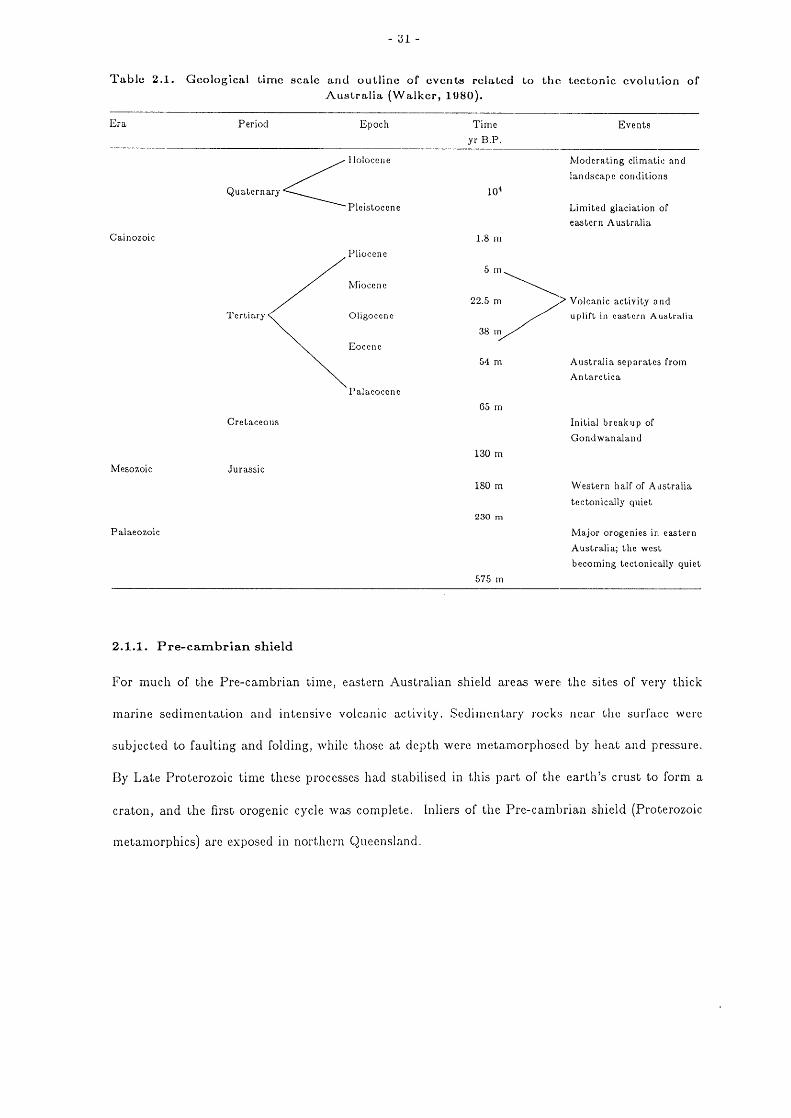
Table 2.1. Geological time scale and outline of events related to the tectonic evolution ofAustralia (Walker, 1080).

Era Period Epoch

Time

Eventsyr B.P.

Moderating climatic and

landscape conditions

Limited glaciation ofeastern Australia

1.8 m

5m

22.5 m J Volcanic activity anduplift in eastern Australia

54 m Australia separates fromAntarctica

65 mCretaceous Initial breakup of

Gondwanaland

Mesozoic Jurassic

Palaeozoic

130 m

180 m

230 m

Western half of Australia

tectonically quiet

Major orogenies in eastern

Australia; the west

becoming tectonically quiet

575 m

38 rn

2.1.1. Pre-cambrian shield

For much of the Pre-cambrian time, eastern Australian shield areas were the sites of very thick

marine sedimentation and intensive volcanic activity. Sedimentary rocks near the surface were

subjected to faulting and folding, while those at depth were metamorphosed by heat and pressure.

By Late Proterozoic time these processes had stabilised in this part of the earth's crust to form a

Craton, and the first orogenic cycle was complete. Inliers of the Pre-cambrian shield (Proterozoic

metamorphics) are exposed in northern Queensland.

- 32 -

2.1.2. Tasman geosyncline

The Tasman geosyncline formed along the east of Australia early in the Palaeozoic and continued

till the Early Mesozoic. Although structural trends varied from region to region, the craton pro-

gressively enlarged in a dominantly eastward direction to the present day limit of the eastern Aus-

tralian continental shelf. The extent of this geological activity is shown in Fig. 2.1, 2.2 and 2.3.

The Tasman geosyncline evolved in three major orogenic cycles. Cambrian and Ordovician

marine sedimentation and volcanism to the south-east of the Pre-cambrian shield exposures ini-

tiated the oldest orogenic cycle; deformation and plutonic intrusion closed it in Middle Ordovi-

cian time.

The next cycle, which began in the Late Ordovician, produced largely terrestrial deposits

from major river systems and was terminated late in Middle Devonian time by widespread uplift.

The youngest cycle, in which the eastern third of Queensland and northern New South Wales were

generated, commenced in Late Devonian time and ended with the Hunter-Bowen orogeny in the

late Permian to Middle Triassic. During this cycle, terrestrial, glacial and marine deposits were

widespread in eastern Australia (Fig. 2.2). Some areas of south-eastern Australia were covered by

land ice during the Permian which modified earlier landscapes (Brown et al. 1968).

As the craton enlarged, subsidence formed basins within the older sequences of metamorphic

rocks, which were filled with predominantly non-marine sediments eroded from neighbouring high-

lands. Extensive sedimentation continued until Late Permian time. Sediments are now mainly

represented by greywackes, shales, slates, phyllites and schists. Earth movements in these basins

during the Permian and Triassic were generally much milder than those of the orogenic belts

which were strongly folded and intruded by acidic magmas and now form most of the present

structural highs throughout the length of eastern Australia.

I I

I

Glacial Deposits

Teiresoial Deposits

Marine Deposits

- 33 -

Fig. 2.1. Cambrian-Ordovician palaeogeog-raphy, showing distribution of land areas ofPrecambrian rocks and of early Paleozoicseas (derived from Brown et al. 1968, Beck-mann 1983).

Fig. 2.2. Silurian to Permian palaeogeogra-phy, showing areas of terrestrial and glacialdeposits (derived from Brown et al. 1968,Beckmann 1983).

Fig. 2.3. Triassic-Jurassic palaeogeography, showing areas of terrestrial and of marinesedimentation, extent of land areas, and mountainous zone on east coast (derived fromBrown et al. 1908, Beckmann 1983).

Paleocene 65 my—40S --

Oligocene 40 my

Miocene 16 my

Pliocene & Quaternary

U U

BroadUpwarps

DDD

Upwarps

—40 S--U

Downwarps

Downwarps

JQ

Downwarps

3

— 40 S — —

Rifts --40

my ___ million years U Upwarps

* Modern position of 40.S

D Downwarps

- 34 -

2.1.3. Extensive Mesozoic basins

Early in Jurassic time, large areas of the craton began to subside, particularly at the sites of older

sedimentary basins. These Mesozoic intra.cratonic basins are evident in extensive areas flanking

the Eastern Highlands and are mainly infilled with fluviatile sediments. The areas to the west of

the Highlands were blanketed by these sediments, which eventually coalesced to form the vast

Great Artesian Basin. The Laura, Maryborough, Nambour and Clarence-Moreton Basins are

eastern counterparts of this basin. The study area represents a section of the Moreton Basin. Dur-

ing the Cretaceous, the sea entered the Great Artesian Basin and the Maryborough and Laura

Basins. (Fig. 2.4). As the sea withdrew about 100 million years ago, deposition in the intracratonic

basins ceased.

Some crustal instability is evident at sites of volcanic activity during the Jurassic and Creta-

ceous. On the east coast, the Clarence-Moreton and Maryborough Basins, were strongly folded

and uplifted, followed by the intrusion of granites and extrusion of intermediate volcanics (the

Maryborough orogeny), while others were virtually undisturbed by earth movements.

Fig. 2.4. Cretaceous palaeogeography, show-ing areas of Lower Cretaceous shallow watermarine sediments and Upper Cretaceous ter-restrial sediments (derived from Brown el al.1968, Beckmann 1983).

Fig. 2.5. Drift of Australia during the Terti-ary (positions relative to 40°S at variousstages shown) and location of major tectonicdisplacements (derived from Beckmann1983).

- 35 -

2.1.4. Mesozoic and Cainozoic uplift

During the Triassic-Jurassic periods, the first stages of the breakup of Gondwanaland resulted in

doming and the first major uplift of the Victorian eastern highlands and Tasmania. These move-

ments preceded the separation of New Zealand from Australia (Wellman 1974). East of the Great

Divide there was intense folding and uplift during the Late Jurassic in the Clarence-Moreton and

Maryborough Basins of south-eastern Queensland, followed by intrusion of granites and extrusion

of intermediate volcanics. This completed the last orogenic movements in Australia (the Marybor-

ough Orogeny). East-west epeirogenic uplifts occurred in Victoria in the Early Cretaceous (Jenkin

1976). Parts of eastern New South Wales experienced major uplift of almost 300 m between the

Mid-Cretaceous and the Late Oligocene (Wellman and McDougall 1974).

The early Tertiary relief of eastern Australia was generally subdued (the Gondwana Surface

of King 1959), but was subjected to prolonged warping and some faulting during the Tertiary

(Oilier 1978). Upwarping to form the Eastern Highlands occurred from Tasmania to Cape York

with complementary troughs intermittantly developed. A continental overview of tectonic dis-

placements during the Tertiary is illustrated in Fig. 2.5.

The nature of the uplift of Eastern Australia during the Mesozoic and Cainozoic has been

the subject of much debate. Three views on the timing of uplift are presented:

(i) Uplift was intermittant with most uplift occurring during the Tertiary. The widely accepted

view of many years has been that vigorous uplift of the Eastern Highlands occurred at the

close of the Tertiary during the `Koscioski Uplift' (Andrews 1910). However, this concept

has been discounted by many workers (Sutherland 1971, Young 1974, Oilier 1978, Wellman

1982). Oilier (1978) contends that evidence of multiple erosion surfaces, the doubtful correla-

tion of duricrusts, and complex drainage patterns, some of Pre-Tertiary beginnings and oth-

ers modified by earth movements and volcanism, refute this view. He came to the alternative

conclusion that most uplift took place prior to or during the Miocene because of the ages of

lava field provinces which appear to be genetically associated with the origin of the Great

Divide (discussed further in Section 2.1.5).

- 36 -

(ii) Over the last 90 million years uplift of the Eastern Highlands has occurred at an approxi-

mately constant rate at any one place (Wellman 1982). It is probable that uplift was slow,

intermittent and varied in magnitude from place to place. In some locations uplift was

about 600 in (Wellman and McDougall 1974), most of it now considered to have been during

Early to Mid-Tertiary time rather than Late Tertiary (Oilier 1978).

(iii) The Eastern Highlands were uplifted to their highest positions during the Cretaceous and

have since been subsiding (Jones and Veevers 1980).

It seems likely that different parts of the Highlands were uplifted at different times (Oilier

1978) but uplift was not necessarily matched by immediate dissection. Where characterised

by major rivers, or soft rock, the Highlands have been deeply dissected (Wellman 1982).

However, in the upper parts of present-day river valleys there are often steps in the river

profile, or the valleys have areas of flat ground above the valley bottom and below the sum-

mits. These features are thought to be due to harder rock having locally restricted the

downcutting of the river or valley side, and not to periods of rapid uplift equal to the

amount of the step, as proposed by King (1959).

In areas of low uplift swamps, lakes and thick sediments have formed (e.g. Lake George and

Omeo areas). In contrast, places of relatively high uplift often formed river gorges (Wellman

1982).

Where widespread uplift formed tablelands, the eastern margins fractured in nearly vertical

faults, giving rise to steep escarpments collectively called the Great Eastern Escapement (Oilier

1982). The main divide is almost always on the western side of the Great Eastern Escarpment,

and the highest mountains are largely drained by easterly flowing streams. Apparently the table-

land rose so slowly that many rivers were able to cut their beds down to keep pace with the uplift.

Now their middle courses run in deep gorges through the highest part of the tableland (Oilier

1982).

Uplift has resulted in the partial stripping of old weathered surfaces of the Eastern High-

lands (Hallsworth and Costin 1953), in canyons in some east flowing streams (Craft 1931), and in

- 37 -

the large volume of Cainozoic alluvia deposited to form extensive plains by west flowing rivers

(Pels 1966, Lawrence 1976, Bowler 1978).

Three theories have been suggested to explain uplift in eastern Australia:

(i) Laserson (1972) believed that the great weight of sediments deposited in the Great Artesian

Basin during the Mesozoic altered the distribution of pressure and stresses in the semi-plastic

undercrust, causing the eastern margins of the Great Artesian Basin to rise while the centre

continued to sink.

(ii) The Eastern Highlands are considered by Oilier (1982) to be a landform of immense magni-

tude related to global plate tectonics. The Highlands are the uplifted western rim of a con-

tinental rift valley with its graben centered in the spreading sea floor of the Tasman Sea and

New Zealand as part of its eastern edge (Fig. 2.6).

(iii) Studies by Ewart et al. (1980) of the chemistry of the more common igneous rocks of eastern

Australia suggest that the molten rock from which they crystallized did not rise quickly from

the source region in the mantle. The molten fraction of the mantle rose to the crust/mantle

interface region and partly crystallized to form a basaltic intrusion, adding to the base of the

crust (underplating). The fluid that did not crystallize later rose quickly to the surface to

form a lava flow. This led Wellman (1982) to suggest that uplift of the eastern highlands

was due to an increase in crustal thickness caused by underplating with subsequent buoyant

upward movement (isostatic movement).

Fig. 2.6. The Western Rift model. A central graben (or sea-floor spreading site) lies between twouplifted blocks, but the axis of greatest uplift lies many kilometres away from the fault scarps.Reversed and disrupted drainage is found on the right hand side of each block. With reference toAustralasia, the left block is eastern Australia, the graben is the Tasman Sea or Coral Sea, andthe right block might represent parts of the Lord Howe Rise, New Zealand, or other sialic frag-ments in the SW Pacific (after Oilier 1982).

2.1.5. Cainozoic volcanic activity

Volcanic activity during the Cainozoic Era was extensive in the Eastern Highlands and began in

the Early Tertiary. It has continued to the Pleistocene and even into the Recent (Laseron 1972),

although Quaternary activity was relatively minor. Most eruptions were coincidental with uplift-

ing of the Eastern Highlands in the Tertiary. Lava flows were mainly of basalt with minor tra-

chyte or rhyolite flows. In some regions, syenite, andesite and trachyte intruded the Mesozoic sed-

imentary beds.

The age of lava flows show that the overall rate of igneous activity for eastern Australia as a

whole has been approximately constant for the last 80 million years (Wellman 1982) although the

older flows are found near the coast and those of younger age inland. Lava flows can be grouped

into provinces from 50 to 200km across. These are distinct regions, with rocks of similar age and

chemistry. Within each province the range in age of the lava generally is less than 5 million years

(Wellman 1982).

-30-

With the exception of one small potassium rich province in New South Wales, all Cainozoic

igneous provinces of eastern Australia are either lava field provinces or central volcano provinces

(Wellman and McDougall 1974).

The lava field provinces were produced from eruptive areas of dyke and pipe swarms up to

100 km across, with widespread flows building shield volcanoes and lava piles up to 1 000 in thick,

almost entirely basaltic in composition. The distribution of lava field provinces appears to be

closely associated with the main divide, and in Queensland they follow the divide rather than the

coastal ranges.

The lava field provinces were most active between 55 and 34 million years ago and there is

some suggestion that active centres of the lava fields have migrated to the west, by distances up

to 200 km (Wellman and McDougall 1974). Oilier (1978) deduced further that if the lava field

provinces are genetically associated with the origin of the divide, then much of the Great Divide

must have attained its position by 34 million years ago and that most earth movements took place

prior to or during the Miocene. Thus the Miocene was possibly tectonically stable with associated

major erosion and weathering, at least along the Divide (Oilier 1978).

Oilier (1978) recognised a subgroup within the lava field province group called areal pro-

vinces. In areal vulcanism, individual volcanoes are short lived, and seldom grow higher than 450

in. Scoria cones, lava cones and maars are the dominant volcanic types and strata volcanoes are

rare. Petrographic composition remains fairly constant. The Australian areal provinces are

characterised by olivine basalt, extensive flows, numerous but small volcanoes and a low explosion

index. They are also the only Australian provinces of Pleistocene age and occur on or near the

line of the Great Divide in western Victoria and northern Queensland (Oilier 1978).

The central volcano provinces are related to large vents, now sometimes represented by

plugs, and were originally volcanic cones up to 1 000 m high, predominantly basaltic with some

felsic flows and intrusions. This type of province is represented in the study area by the Main

Range Volcanics (Stevens 1965). Their chemistry and differentiation history differ from the lava

field provinces (Wellman and McDougall 1974). The central volcano provinces were active between

6,

- 40 -

33 million years ago and 6 million years ago and there is a remarkable correlation of age with lati-

tude. When plotted on a map, they are seen to fall roughly into two lines and become younger to

the south (Fig. 2.7). Wellman and McDougall (1974) suggest that this phenomenon resulted from

the Australian plate moving in a northerly direction over two magma sources (hot spots, melting

spots, plumes) fixed in the asthenosphere beneath the crust. On this evidence, East (1986) sug-

gests that volcanism and probably uplift are both causally linked with the opening of the Tasman

Sea and the Southern Ocean, and the associated tensional stresses in the lithosphere.

Fig. 2.7. Map of central volcano provinces of Australia. Numbers refer to potassium-argon age inmillions of years (data from Wellman and McDougall (1974)). Source: Oilier (1978).

- 41 -

2.1.0. Tertiary sedimentation

Marine Tertiary deposits were of minor extent and are associated with a series of basins along

Bass Straight and also the Murray and St. Vincent Basins (Brown et al. 1968). Terrestrial deposits

were much more widespread, particularly in major drainage basins within the Eastern Craton (Fig.

2.8).

Fig. 2.8. Simplified representation of major elements of the early Tertiary landscapes of Australia(Beckmann 1983).

The drainage basins were of two main types (Beckmann 1983):

(i) Those within the Eastern Highlands belt include quartzose gravels, shales, sandstones and

clays with interbedded volcanics (Beckmann and Stevens 1978). In North Queensland, the

extensive Karumba Basin of the Carpentaria region developed, as did a number of smaller

basins along the Eastern Highlands and in inland North Australia. No Tertiary sediments

have been mapped within the study area, although minor deposits are associated with the

Main Range Volcanics (Cranfield et al. 1976).

(ii) Those associated with inland drainage systems. These include both intracratonic basins such

- 42 -

as the Lake Eyre Basin and older basins such as the Georgina, Drummond, Amadeus and

Upper 'Murray, which resulted from renewed sagging in the Early Tertiary.

2.1.7. Cycles of Cainozoic weathering, erosion and deposition

The northern drift of Australia to essentially its present latitude occurred before the latest major

accumulation of ice in Antarctica (Kemp 1978). Thus, compared with many parts of the northern

hemisphere and New Zealand, soil renewal in many Australian landscapes, through erosion by

flowing water and glacial action and through the accession of fresh minerals by volcanic or tec-

tonic activity, has been minimal (Walker 1980). Locally, however, less weathered basaltic materi-

als exposed by subsequent erosion have provided parent material for fertile soils as found on the

Darling Downs and Lockyer Valley in Queensland. This is a characteristic feature of the study

area.

Given the geological framework outlined in Table 2.1 many eastern Australian landscapes

and soil parent materials would be expected to be of great age. Palaeomagnetic studies of weath-

ered zones (Idnurm and Senior 1978) and K-Ar dating of basalts overlying such weathered zones

(Coventry 1979; Dury and Langford - Smith 1969) support these expectations. Deep geochemical

weathering of rocks, particularly basalt, during the Tertiary provided the eastern Australian

landscape with an abundant supply of material susceptible to fluvial processes. Deep weathering of

a planation surface in western Queensland commenced in the Cretaceous and continued into the

Palaeocene (Day et al. 1983). This resulted in the formation of the kaolinised, ferruginised, mot-

tled and silicified Morney Profile which has been palaeomagnetically dated at GO ± 10 million

years (Idnurm and Senior 1078). This profile is now only preserved in inland regions but isolated

silcretes in eastern regious may date back to this period. However, many of these silcretes under-

lie Mid-Tertiary basalts and may be due to later weathering of the volcanic rock (Day et al. 1983).

Tectonic activity in eastern Australia slowed in the Eocene, allowing extensive planation sur-

faces to develop in many areas. During the Oligocene, these surfaces were deeply weathered to sil-

iceous and ferruginous duricrusts (Day et al. 1983). The most extensive of these was the inland

- 43 -

Cordillo Surface (Wopfner 1974).

Extensive earth movements and basalt flows in the Oligocene and Miocene resulted in the

development of new centres of deposition. A post-basalt erosion surface developed in the south-

eastern region of Queensland (Day et al. 1983). An extended period of weathering in Late Miocene

time was marked by the development of deep lateritic weathering profiles on post-basalt, erosion

surfaces.

Other periods of lateritic weathering have been recognised in several locations (Browne 1969,

Grimes and Doutch 1978), including the study area (Watkins 1967), but these were not as pro-

longed as the Late Miocene event and their effects are not as widespread. As a result, landscapes

were easily eroded and yielded considerable sediment as climate changed through the Late Terti-

ary into the quaternary.

On the tablelands various 'cycles' or 'sequences' of local landscape developments have pro-

gressed by peneplanation, pediplanation, etchplanation or by other processes (Oilier 1982). The

history is not entirely erosional, and periods of flu-vial aggradation and extensive lava flows have

periodically built up the landscape. It appears that much of the tablelands were relatively flat

with a relief of a few hundred metres for very long periods. In contrast, the coastal belt has a

more consistent history of downcutting, with retreat of the main escarpment creating a complex,

diachronic surface on the coastal lowlands (Oilier 1982). This situation applies to the study area,

in which east flowing streams have incised into a tableland forming escarpments in the headwater

regions and complex valleys of gentler relief downstream.

The shape of the scarp in plan, with deep embayments along valleys and peninsulas along

interfluves, suggests that the scarp is moving backwards from the cast coast by fluvial erosion and

irregular scarp retreat (Oilier 1982). This massive landscape feature was possibly initiated when

chasmic faults created a new continental edge and a new base level of erosion. As yet there is no

continental correlation of erosion surfaces, although regional surfaces have been established. Van

Dijk (1984) has suggested there is geomorphic evidence of equivalent soil landscape development

in widely separated parts of the Murray-Darling River catchment. Weathering features beneath

- 44 -

the solum of cracking clays are believed to characterise stages of landscape development and soil

weathering from Mid-Tertiary to Pleistocene times.

Multiple erosion surfaces are undoubtedly present in eastern Australia, and in any region,

some may be better developed than others. However, the concept of a single erosion surface

extending simultaneously over all eastern Australia (e.g. the Australian Surface of King, 1959) is

highly unlikely (Oilier 1978).

Despite certain anomalies 011ier (1982) suggested a relative chronology for eastern Australia

beginning with the erosion of plains, followed by initiation of major river patterns, widespread

basalt flows, uplift and formation of the Great Divide, and finally formation and retreat of the

Great Escarpment.

Modern drainage patterns and valley forms in eastern Australia were established by tectonic

uplifts and up-and down warps during the Late Cainozoic (Beckmann 1983). New surfaces were

exposed during backwearing of scarps away from major river systems and the remnants of older

surfaces above the widespread Early Tertiary surfaces were further reduced (Beckmann 1983).

The deeply weathered Tertiary surface(s) were eroded, leaving only parts of the original surface.

For example, the margins of the Karumba Basin in Cape York Peninsula were uplifted in the

Pliocene resulting in extensive fan development and five stages of deposition have been identified

(Grimes and Doutch 1978). Another example is the Fitzroy River catchment of central Queens-

land, which consists of extensive undulating lowlands, low ranges and high dissected sandstone

plateaux. Geomorphic studies (Galloway 1967a, 1967b; Wright 1968) indicate a Tertiary mantle

up to 70 m thick, mainly made up of terrestrial deposits which once covered most of the region.

During the Tertiary this mantle was intensely weathered and developed deep laterite profiles

which were subsequently eroded. By the Late Tertiary the landscape took on its present form.

All that remains of the original Tertiary surface are undulating plains and low plateaux. Materi-

als exposed by partial stripping and redeposition of the deeply weathered mantle occupy large

areas, as do extensive alluvial plains of more recent origin.

- 45 -

In the lowlands of western Queensland, East (1986) describes how the duricrusted surface of

the Great Artesian Basin was subjected to broad warping toward the end of the Tertiary. In

upwarped regions, a new cycle of erosion was initiated with the development of extensive apron-

like sheets around the bases of aligned mesas, cuestas and tablelands, and the infilling of interven-

ing valleys.

Relief inversion occurred locally with the formation of synclinal uplands. On these erosional

landsurfaces, the main drainage was largely confined to narrow synclinal belts in well defined

linear floodplains. Thus post-duricrust earth movements influenced drainage patterns as they fol-

lowed the regional tectonic grain.

In south-east Queensland, where the study area is located, the Great Divide lies on the

Miocene surface on lateritized basalt. It was cut down during the Late Miocene and Pliocene, and

a succession of younger surfaces were developed at various stages of dissection (Watkins 1967,

Beckmann and Stevens 1978). As earlier surfaces were reduced, lineament and structures of the

underlying rocks controlled stream direction and the central position from which younger surfaces

extended with time (Beckmann and Stevens 1978). Two major surfaces, each with a base level

only a few tens of metres above present sea level, indicate slight regional uplift in the Late Caino-

zoic. These surfaces were further dissected during subsequent periods of low sea level.

In New South Wales, large valleys were carved out below the level of the Miocene surface

and the extent of the new surfaces formed during the Pliocene depended on original elevations of

the older surfaces (Browne 1969). These modified Pliocene valleys, both east and west of the

Divide, have cut back so far that valley walls are virtually coincident with the Miocene surface

boundary (Beckmann 1983).

Late Cainozoic uplift and erosion in eastern Victoria extended Mid-Cainozoic downcutting

on the southern side of the Eastern Highlands, but there has been insufficient time for distinct ero-

sion surfaces to develop, especially on the northern side (Wellman 1974). Any identifiable erosion

surfaces in the east may be due to differential erosion of rocks of varying hardness (Wellman

1979).

- 46 -

2.1.8. Late Cainozoic changes in sea level

During the Late Cainozoic, custacy had a decided influence on eastern coastal streams and pat-

terns of alluvial deposition. Glaciations lowered sea levels and induced valley cutting by coastal

streams, while the melting of ice in the Pliocene caused inundation of the Lower Murray River

Valley (Beckmann 1983). In some coastal regions eustatic effects were superimposed on those of

tectonic events e.g. Gippsland area in Victoria (Ward et al. 1971) and the Karumba Basin in

North Queensland (Doutch 1976).

Times of low sea level during interglacial periods resulted in the exposure of the eastern con-

tinental shelf to a maximum depth of more than 100 m below present sea level. The lowering of

sea level closed both the Torres Strait and the Bass Strait (Jennings 1971, Galloway and Loeffler

1972) and produced temporary barriers to ocean circulation on several occasions (Gill 1962). In

response to the lowered base level coastal valleys were excavated (Beckmann 1983).

With each rise in sea level, coastal valleys were drowned and filled with sediment, commonly

to a level below the previous infilling (Beckmann 1983). Rising sea levels caused a series of low

level benches to be cut along the coast during the Late Quaternary (Langford - Smith and Thorn

1969) and New Guinea and Tasmania and smaller islands were separated from the mainland.

With each cycle of sea level rise and fall, alternating cycles of valley infilling and stream

rejuvenation occurred, forming terraces near coastal river mouths. These were continuous with

terraces resulting from climatic change (Beckmann 1983). Heights of sea level rises were generally

believed to be less than 6 m above present, suggesting Late Pleistocene or younger age. Only

occasional alluvial remnants exist above these heights (Beckmann 1983). In North Queensland,

alluvial plains of coastal rivers contain material which may be Late Tertiary or Pleistocene in age

(Lucas and de Keyser 1965). High level alluvia along the coast to the south may be of similar age

(Beckmann 1983).

The effect of Quaternary sea level variations on coastal fluvial landforms has been observed

in various parts of eastern Australia (Warner 1972; Coventry et al. 1980). Quaternary stands of

sea level must have been synchronous around Australia and provide a unifying principle for the

-47-

study of coastal fluvial landforms and processes. Too few data are available at present for a

comprehensive statement, to be made about eastern Australian Quaternary coastal floodplains

(Walker 1984). Correlations of alluvial bodies along the eastern coast are difficult even though

heights may be similar, as there may have been local variations in the amount of tectonic uplift.

2.2. Climate

It has been established from palaeohydrological and palaeobotanical evidence that the Australian

climate varied considerably during the Tertiary and Quaternary. However, patterns of climatic

change over time across Australia have not been uniform because of differing regional physiogra-

phy (Beckmann 1983). The distribution of mountains and plain, the effects of varied relief on

movement of pressure systems, the degree of continentality and interruptions to oceanic circula-

tion at times of low sea level are all contributing factors to regional climate.

Rather than being affected by alternating periods of glaciation, Australia has been subjected

to past cycles of moist and arid conditions relative to the present (Bowler et al. 1976; Kemp

1978). As a result of these cycles, widespread erosional instability was induced during the Quater-

nary (Walker 1984). Thus episodic fluvial erosion and deposition is associated with Quaternary

climatic change (Bowler et al. 1976, Coventry et al. 1980).

Recent soil and landscape studies based on radiocarbon dating indicate an intense episode of

fluvial erosion and deposition in the south-east highlands prior to the peak of the last glaciation,

between 20 000 and 30 000 years ago (Costin and Polach 1973; Coventry and Walker 1977;

Walker and Gillespie 1978). Dates from a range of sites in south-eastern Australia also led Willi-

ams (1978) to identify another less intense erosive/deposition episode about 1 500 to 4 000 years

ago. It seems probable therefore that significant, climate changes in the Late Quaternary have

resulted in some synchronous changes in fluvial landscapes and soils in parts of south-eastern Aus-

tralia (Walker and Butler 1984). Drier climates during the last glaciation are also in evidence for

tropical eastern Australia (Bowler et al. 1976; Kershaw 1978) although their relationship to fluvial

landscape behaviour is yet to be established.

- 48 -

The changes in climate in eastern Australia are summarised below from Galloway and Kemp

(1981) and Kershaw (1981).

The Early Miocene was warmer and wetter than that experienced today over extensive areas

of eastern Australia. There was deep interior penetration of rains with an annual rainfall of 1500-

1800 mm estimated from botanical fossil evidence. This climate was responsible for widespread

deep weathering of rocks.

Temperatures fell in the Middle Miocene as ice rapidly accumulated in Antarctica with a

marked drop in the Late Miocene (Wellman 1982). Warming seas followed in the Early Pliocene

(3.9-4.3 million years ago) with the onset of a strongly developed dry season at the end of the

Pliocene.

Early and Middle Pleistocene climates seem to have been dominantly dry. Lacustrine and

aeolian sediments in the Lower Murray Valley record an irregular trend from humid to generally

dry conditions, and aeolianite and palacosols imply interglacial conditions not vastly different from

those of the present.

For the Late Pleistocene, pollen profiles of Lake George near Canberra indicate for the

period 350 000 to 140 000 years before present (BP) alternating dry cold climates and warmer

moister climates corresponding to interglacial periods. For the period 140 000 to 65 000 I3P,

eastern Australia experienced a sequence of temperature rises and increasing precipitation with an

extension of forest vegetation. Subsequently there was a sharp climatic deterioration with reduced

rainfall and temperatures resulting in grassland expansion in the south. At the same time closed

araucarian forest and open woodland began replacing complex closed forest on the Atherton

Tableland (Kershaw 1981).

Fairly detailed climatic reconstruction for eastern Australia in the Late Quaternary has been

attempted by Bowler et al. (1976) and Rognan and Williams (1977). A palaeoclimatic chronology

based on their data is presented below:

60 000 -40 000 years BP. The entire length of eastern Australia was drier than at present.

Inland lakes were dry for long periods.

-.19-

40 000-30 000 years BP. In southern Australia, cool to cold conditions prevailed, reduc-

ing evaporation and increasing effective rainfall. This resulted in higher lake levels and

greater fluvial activity with high bedload regimes.. In contrast tropical north Queensland

became drier and cooler.

80 000-25 000 years BP. Glaciers became active in Tasmania and in the Southern Alps.

I-ligh lake levels in southern Australia were sustained by a continuation of pluvial conditions.

Aridity persisted in north Australia.

25 000-15 000 years BP. Glaciation peaked and began to decline 20 000 years ago in the

Snowy Mountains and about 14 000 years ago in Tasmania. Rainfall became lower and

lakes in southern Australia contracted. Lake levels were briefly high, probably about 20

000-18 000 years BP presumably due to melt waters of the retreating snow and ice. Develop-

ment of both clay and sand dunes derived from lake and ancestral stream margins in the

southern interior were most active during this cold arid period. hi tropical eastern Australia

this period was the period of greatest dryness.

15 000-10 000 years BP. A brief pluvial episode from 15 000-14 000 years ago resulted in

a temporary rise in southern Australian lake levels. Otherwise conditions were relatively dry

but more pluvial than the preceding period; lake levels were low and previously formed

dunes were stabilised. Aridity continued in northern Australia. This period is considered to

be a period of transition between arid earlier conditions and later humid ones.

10 000 years BP to present. Ice finally disappeared in Tasmania. There was increased

rainfall and temperatures with a rise in lake levels throughout eastern Australia. This

period has been a period of relative climatic stability although rainfall was marginally higher

from 8 000 to 6 000 years ago. A decrease in effective and absolute precipitation has

occurred since then.

While a great deal is known about climate in the northern and southern extremes of eastern

Australia, little information is available for Quaternary climates in the mid-latitude regions of

southern Queensland and northern New South Wales. The study area is located in this region.

- 50 -

2.3. Current river systems

A general model for Australian fluvial systems (Fig. 2.9) has been developed by Walker and Butler

(1983). The general distribution of these systems is highlighted in Fig. 2.10, in which modern

rivers are characterised by the presence or absence of certain landscape components (Walker and

Butler 1983). Some river systems such as the Murray-Darling system have all these components

and are thus designated WRLO. Others such as the Diamantina and Finke drain into Lake Eyre

and have no 0 component (WRL).

Upper catchmentsdominated by hillslopes;

some fans and terraces

Riverine plains and river terraces dominant;some tow hillslopes

Riverine flood plains dominant;lakes and aeolian landforms

Coastal plains and estuaries

Sediments dominatedby bedload

Sediments dominated by overbank deposits;suspended load and solutes

Sediments dominated bysuspended load and solutes;

aeolian clays and sand

Sediments dominated bysuspended load and solutes

0LR

Fig. 2.9. General fluvial systems model showing the four major landscape components W, R, L, 0and associated features (Walker and Butler 1983).

Except for central Queensland, most east flowing streams are designated as WO, whereas

west flowing streams have a range of river systems. In south-eastern Queensland where the study

- 51 -

area is located, a WRO rather than a WO river system is found (Fig. 2.10).

Fig. 2.10. Areas of Australia in which the river systems are classified after Walker and Butler(1983) according to the presence of certain fluvial landscape components.

W = watershed (hillslopes) where overland flows dominate;R = riverine landscapes where channel and overbank fluvial processes dominate;L lacustrine influence on stream flow and fluvial transport;

0 = river systems terminating in the ocean.

The coastal WO river systems of eastern Australia pass largely through hilislope terrain

before reaching the ocean. They are either short fast flowing perennial streams cutting sharp

tracts through the highlands or slower tributaries of large river systems. Varying degrees of estua-

rine or deltaic plains plains developed as coastal valleys were drowned following the last glaciation

(Walker and Butler 1983). Wide alluvial plains of major rivers rarely exceed 60 m above sea level

on the Queensland coast (Queensland Resources Atlas 1976).

In contrast to the coastal streams with steep watersheds from uplifted highlands, inland

streams are generally associated with moderate relief. The flat lying sediments of the Great Arte-

sian Basin are responsible for the subdued more uniform character of the western plains.

- 52 -

A review of river patterns reveals that most of the river systems of eastern Australia have

complex geomorphic histories (Oilier 1978). Strike valleys, river capture, drainage patterns

modified by folding and/or faulting, volcanic disruption of drainage patterns and subsided con-

tinental edges can be found in eastern Australia. Some drainage patterns can be traced to early or

pre-Tertiary beginnings while earth movements and vulcanism have modified drainage patterns at

many different times, probably throughout the Cainozoic (Oilier 1978).

The influence of Quaternary tectonics on fluvial landscapes appears to have been of minor

local significance e.g. Bowler and Harford (1066) in the Riverine Plain of south eastern Australia

and Pillans (1974) cited by Walker (1984) in the erosional uplands of the Murrumbidgee River.

However, Walker (1984) suspects that Quaternary tectonics have probably been underestimated as

a geomorphic factor in Australia.

Entrainment and differential transport and deposition of Tertiary weathering products dur-

ing the Quaternary were generally accomplished by river systems of low gradient traversing dry

climatic regions. The low sediment delivery of these streams has meant that much of inland Aus-

tralia is characterised by alluvial fans and extensive depositional plains of Quaternary age (Walker

1984).

Throughout eastern Australia it is apparent that episodic landscape development occurred

during the Quaternary in response to climate changes ranging from arid to humid tropical (Table

2.2). Fluvial landscape development is more commonly explained by changes in climate rather

than by tectonics or fluvial responses to sea level changes (Table 2.2). In the Riverine plain and in

valleys along the eastern highlands, fluvial landforms and sediments are dominantly of Quaternary

age (Walker 1984). By contrast, some fluvial deposits in western Australia are essentially Tertiary

in age (Mulcahy and Bettenay 1972).

In the upper reaches of eastern Australian drainage systems, evidence of episodic alluviation

are seen in flights of stream terraces, but their origins are unclear. Determining the origin of ter-

races requires assumptions about channel section and morphology, kind and rate of supply of sedi-

ment load and climatic parameters of rainfall and temperature (Walker 1984). More detail about

- 53 -

these variables in relation to modern rivers is required to improve our understanding of Quater-

nary terraces and associated river channels.

Where extensive alluvial plains deposition has occurred throughout the Quaternary, alternat-

ing coarse and fine sediments have been deposited and soils have developed on stable surfaces

until truncated and/or buried by more sediment. The palaeoenvironmental interpretation of such

sequences remains unclear, partly because of the lack of specific environmental signatures in

fluvial sediments (Walker 1984). As in the case of river terraces, explanations of varying river

regimes and related sedimentation in alluvial plains require more detailed studies of modern river

processes (Walker 1984).

Table 2.2. Summary of characteristics and processes proposed for Quaternary fluviallandscapes at a range of locations in eastern Australia. (Adapted from Walker 1084).

Location River systems* Dominant fluvial

landforms

Formative

factors

Reference

North eastern

Australia

WO, WHO Eroded Tertiary surfaces,

alluvial fans;coastal and

inland alluvial plains

Eustatic movements;

climatic change;

tectonics

Coventry et al. 1980

North coast,

N.S.W.

WO River terraces; coastal

flood plains

Eustatic movements;

climatic change

Warner 1972

Upper Darling

River

WRLO Extensive clayey flood plains Climatic change;

tectonics

Taylor 1978

Southern highlands,

coast of N.S.W.

WO, WRLO Alluvial fans; river terraces,

localised flood plains

Climatic change Walker Coventry

1976

South eastern WO Late glacial alluvial fans Climatic change Wasson 1977

Tasmania

Eastern Tasmania WO River terraces and flood

plains

Climatic change Nicolls 1960

Lower Murray - WRLO Extensive clayey flood Climatic change; Butler et al. 1973

Darling Basin plains tectonics

Arid Sou th

Australia

WRL Alluvial fans Climatic change;

tectonics

William 1973

* The code for the river system designations is given in Fig. 3.9.

A characteristic feature of many extensive alluvial plains in eastern Australia is the

preponderance of clay rich sediment (Butler 1958, Taylor 1976 cited by Rust 1981). The reason

-5-1-

for this dominance in large river systems is little understood, nor have the conditions of overbank

deposition of very fine sediment been critically studied (Walker 1984).

2.4. Alluvial soil landscapes

The variable nature of geological source materials, combined with differences in climatic history,

topography and differential erosion of old weathered profiles have resulted in a wide variety of

soils on alluvial landscapes in eastern Australia. In a summary of soil distribution of the Moreton

Region, south-eastern Queensland which includes the study area, Hubble and Isbell (1983) describe

a range of soils on alluvial landscapes. Significant areas of deep black earths are indicated on

dominantly basaltic alluvia together with prairie soils, grey clays and red brown earths. Where

there is little basaltic component, solodic soils are common on the highest terrace while mixed

alluvial soils and weakly developed prairie soils occur on lower terraces. On older terraces and fan

alluvia out of ferruginous quartzitic sandstone, red earths are common, while on very old alluvia,

lateritic podzolics are evident. On the poorly drained coastal plains, extensive areas of humic

gleys and minor gleyed podzolic soils occur.

In other alluvial landscapes of eastern Australia, the CSIRO Division of Soils (1983) have

described different suites of soils. For the purposes of comparison, details on other alluvial soil

landscapes in eastern Australia are presented in Appendix 1.

- 55 -

3. STRATEGIES FOR INVESTIGATING ALLUVIAL SOIL LANDSCAPES

3.1. Introduction

The soil age relationships in any landscape help to explain soil physical and chemical characteris-

tics, duration and intensity of pedogenic processes and even management of soil resources (Finkl

1984). In alluvial landscapes, an understanding of soil stratigraphy and history requires the

identification, characterisation and ranking of equivalent alluvial strata, often on a range of

different landforms and sediment facies.

Following deposition, alluvium may be subjected to soil forming processes and, initially, to

the process of ripening. Ripening is the term given by Pons and Zonneveld (1965) to the first

stage of weathering and evolution of soil from raw alluvium or other water laid deposits exposed

to air for the first time. The processes are mostly irreversible (Oilier 1969). Ripening of alluvium

in the Netherlands has been described by Pons and Zonneveld (1965). The fresh alluvium loses

water by compaction, evaporation and transpiration. This results in an increase in attraction

between soil colloids, causing consistency to increase, the volume of mineral component to be

reduced and the relative proportions by volume of several soil compounds change. Swelling of

particles by later wetting reduces water uptake, and prevents the soil from acquiring the original

unripe state. As physical ripening proceeds, chemical ripening occurs, involving mainly oxidation,

cation exchange on the clay and decalcification. In addition there is biological ripening which con-

sists of microbiological alteration and mixing by soil fauna. Other soil forming processes then fol-

low that result in organic accumulation, chemical weathering and reorganisation, translocation

and concentration of the more mobile constituents due to the effects of the environment (Brewer

1964).

Pedogenesis may be interrupted either by burial of the soil below the depth of pedogenesis

or by erosion of the deposit. The longer the alluvium is exposed at the surface, the greater the

progress of pedogenesis until the soil so formed reaches either equilibrium with its environment, or

a steady-state. Old soils exhibit quite different properties to recently formed soils developed from

- 56 -

similar sedimentary parent material. Thus soil age is an important concept in the study of allu-

vial soil stratigraphy for relating laterally extensive and stratigraphically equivalent bodies of soils

to other such bodies. This is a natural extension of the time factor of soil formation as recognised

by Jenny (1941) in his equation of soil formation.

Soils formed on a past landscape are termed palaeosols (Ruhe 1969) and may be buried or

exposed. Palaeosols on exposed surfaces are termed relict while in rare cases a palaeosol may be

re-exposed by denudation (exhumed). Buried palaeosols may be difficult to identify due to the

transitory nature of many soil features and their liability to post burial alteration (Valentine and

Dalrymple 1976). The similarity in the processes and products of pedogenesis to those of

diagenesis may confuse the recognition of buried palaeosols. There are very few features that are

unique to terrestrial soils as opposed to sediments. Morrison (1978) has recognised three situations

in which palaeosols develop. Soils with evidence of more than one episode of pedogenesis within

the same profile are termed composite (this term appears equivalent to polycyclic). Where an AB

soil profile closely overlies another, but they are separated by sediment and individual soil profiles

do not overlap, Morrison called these compound palaeosols. The whole sequence may be also

termed a multistorey profile. Where composite soils are traced laterally to places where they are

separated by sediments into two or more profiles, these are called subdivided palaeosols.

Recognition of pedogenic relicts associated with palaeosols is essential to soil stratigraphy.

Relationships between palaeosols, deeply weathered substrates and modern soils indicate that

many contemporary soils contain relicts which have developed in a palaeosol (Finkl 1980). Such

features may be used as guidelines to determine relative age.

3.2. Principles of soil stratigraphy

The following principles relevant to alluvial landscapes have been largely summarised from Fink!

(1980). These concepts are considered as aids to understanding the episodic development of the

soil continuum, rather than established 'earth laws'. Rather than assuming a simple pedogenctic

relationship between successive horizons or layers in a soil, it is necessary to first understand the

- 57 -

erosional and depositional history of the landscape, and then to interpret horizon relationships

(Walker 1980). Invariably there are gaps in the required stratigraphical evidence.

3.2.1. Law of superposition

In any undisturbed sequence of sedimentary strata., the youngest stratum is at the top and the

oldest at the base (Gary et al. 1074). Older strata are successively overlain by younger and

younger layers. A corollary to this law it that a deposit can be no younger than the soil developed

in it, but may be much older. Conversely, the soil can be no older than the parent material in

which it is developed but can be much younger.

3.2.2. Separate identity

Procedures used by geologists to distinguish sedimentary layers have been successfully applied

where soil layering is suspected. Soil stratigraphic layers are more complicated than purely sedi-

mentary layers due to pedogenic factors introduced during weathering.

Proofs of the independent nature of layers have been referred to by Walker (1958) as the

`principle of random association', by Morrison (1967) as 'separate identity' and by what Butler

(1959) terms the 'principle of association'. All these principles emphasise that the separateness of

a layer is established by showing changes in the morphology or constitution between successive

layers and by demonstrating that vertical trends within superposed layers are independent of each

other. Analyses of vertical trends may involve lithological, mineralogical and morphological

discontinuity between layers and the concept of reverse weathering differentials, where less weath-

ered surface materials overlie strongly weathered materials (see Section 2.3.1).

3.2.3. Lateral continuity

Lateral termination of sedimentary bodies may result from erosion, or it may progressively thin to

extinction, interdigitate or gradually merge with other deposits (Krumbein and Sloss 1963).

Where sedimentary layers and soils developed in them are separated by stone lines, lateral con-

tinuity of the weathered layers is apparent. Stone lines in soils may indicate that soil

- 58 -

development has taken place in more than one parent material i.e. the soil formation straddles a

lithologic discontinuity (Ruhe 1959). Iii this case the soil profile above the stone line represents a

separate younger phase of soil development than the in situ profile below the stone line. The soil

below the stone line has been subjected to post burial soil formation. The result is called a welded

profile (Ruhe and Olson 1980).

However stone lines are by no means unequivocal evidence that sedimentary layering has

occurred. Termites were concluded to be responsible for stone lines found in Ugandan soil profiles

(Oilier 1959). Ancillary to lateral continuity is the concept of lithologic transgression. Weathering

at the earth's surface transgresses both lithologic and pedologic boundaries. The imprints of soil

development in transported (sedimentary) parent materials may mask the lateral continuation of

soil layers (Leamy 1975). Facies* within sedimentary layers also need to be comprehended

* Facies - deposit distinct from neighbouring, contemporary ones because of differences in depositional environment

(Hunt 1972).

in attempts to follow soil stratigraphic units laterally.

3.2.4. Ascendancy and descendancy

According to the principle of ascendancy, a hillslope may be the same age or younger than the

higher surface to which it ascends. The principle of descendancy, states that a hillslope deposit is

the same age as the alluvial fill to which it descends (Finkl 1980). This principle makes it possible

to date pedogenic events in stratified materials from dated soils located elsewhere in a landscape.

3.2.5. Pedogenic persistence

Yaalon (1971) classified pedogenic processes into 3 groups based on their rates of reaction. The

mode of origin and relative persistence of soil features associated with these processes are listed in

Table 3.1.

- 59 -

Table 3.1 . Soil diagnostic features and horizons grouped according to their mode of originand relative persistence in palaeosols (after Yaalon 1071).

Altered easily, Relatively persistent

Persistent features**

generally < 103 years to slowly adjusting.

reach steady state generally > 103 years to

reach steady state

Properties acquired by reversible, Mostly steady-state near-equi- Features produced by essentially

largely self-regulating processes

librium features or metastable

irreversible, self-terminating

state processes

Mollie horizon (f)*

Slickensides (c)

Salic horizon (c)

Gypsic horizon (o)

Mottles (c)

Gilgai features (c)

Cambic horizon (o)

Spodic horizon (o)

Cambic horizon (f)

Umbric horizon (f)

Spodic horizon (f)

Fragipan (f)

Mottles (o)

Argillic horizon (c)

Natric horizon (o)

Calcic horizon (f)

Gypsic horizon (c)

Histic horizon (c)

Oxic horizon (f)

Placic horizon (f)

Plinthite (f)

Durinodes (1)

Petrocalcic horizon (f)

Gypsic crust (f)Argillic horizon (c)

Natric horizon (c)

Albic horizon (o)

Fragipan (o)

Histic horizon (o)

* Definitions of horizons and features according to the American classification system. Letters in parenthesis are an at-

tempt to evaluate semi-quantitatively the frequency or persistence of the feature within the group: f-frequently; c-

commonly; o-occasionally; r-rarely. Some features are listed in two groups. Most features could be listed in all remaining

columns with the connotation (r).

** Subdivision into features with influx exceeding efflux and those with efflux exceeding influx can be made, but was not

deemed necessary in the present context, for evaluation of persistence in palaeosols.

Many soil forming processes are feedback processes which are self-accelerating because of

continuous reinforcement of the causes starting them. De-acceleration and finally termination of

the feedback mechanism occurs when one of several factors (or reactants) in the process become

limiting (Torrent and Nettleton 1978). An example of this is the depletion of easily weatherable

minerals causing the cessation of soil formation.

Soil features which persist for long time periods through changing conditions of soil forma-

tion are the result of essentially irreversible, self terminating processes (Yaalon 1971). The dur-

able nature of persistent soil features despite environmental change, has been termed pedogenic

inertia (Bryan and Teakle 1940). Pedogenesis either lags behind these changes or has continued

beyond certain chemical and physical thresholds to become irreversible.

Yaalon (1971) believes rapid transformation of organic carbon and nitrogen following burial

is the main reason why so few mollic horizons have been recognised in palaeosols. Metastable

- 60 -

processes such as the development of argillic horizons or humus iron pans of podzols developed in

sands may require 102-103 year time intervals (Fink' 1080). The formation of thick mottled and

pallid zones of deep lateritic profiles may need 106-107 years (Whitehouse 1940, Idnurm and Senior

1978). Many irreversible, self-terminating reactions show remarkable stability and persist for long

periods. Petrogypsic and petrocalcic horizons have extremely high durability in ancient hard crust

landscapes (Goudie 1973) as have iron duricrusts in cratonic regions (Finkl 1978). Such duricrusts

may be important in interpretations of landscape evolution because they represent critical stages

in pedogenic history, and have a subsequent effect on the erosion/sedimentation cycles that follow

(Fink' 1979).

3.3. Soil stratigraphic units

Various studies have led to the definition of a number of soil stratigraphic units such as palaeosols

(Ruhe 1969), pedolith (Crook and Coventry 1967), pedomorpholith (van Dijk et al. 1968), geosol

(Morrison 1978), pedoderm (Brewer et al. 1970) and grou:ndsurface and K layer (Butler 1959).

These differ from each other in detail, but have the same central concept of a laterally extensive

body of soil formed by pedological alteration (due to exposure at the earth's surface) of a rock

stratigraphic unit or a sequence of superposed rock units (Brewer 1972).

Brewer et al. (1970) suggest a type transect rather than a type site to characterise a soil stra-

tigraphic unit; this allows for assessment of the geographical variation of buried units, as geneti-

cally similar soils at close but different stratigraphical levels may be miscorrelated. These con-

cepts are particularly useful when applied to alluvial landscapes.

It is accepted that periods of erosion and deposition, followed by soil formation occur in

episodic cycles (K cycles, Butler 1959). Soil stratigraphic units, often superposed one on another,

can thus be recognised by their degree of soil formation and their stratigraphic and age relation-

ships (Brewer .1972). However, separation of soils on a chronostratigraphic basis requires careful

application of absolute and relative dating methods (Finkl 1984). Pedogenic relationships between

successive horizons or layers in a soil may not be assumed until the erosional and depositional his-

- 61 -

tory of the site are understood. Brewer (1972) indicated three difficult situations in regard to

placement of soil units into a stratigraphic sequence and especially in assigning isotopic ages:

(i) where sediment deposition has been so slow that pedological alteration was significant during

deposition,

(ii) where continuous gradual erosion occurs during soil formation (the steady state of Nickiferoff

(1959)),

(iii) where time of deposition may vary gradually in a lateral direction over the areal extent of

the sedimentary body.

The existence of these situations emphasises the importance of a knowledge of soil stratigra-

phy in studies of soil genesis. Without such knowledge, superposed stratigraphic units may be

misinterpreted as soil horizons and differences between adjacent soils may be erroneously attri-

buted to factors other than time.

3.3.1. Recognition of buried soil stratigraphic units

From our present knowledge of soil forming processes, many soil properties can be expected to

show characteristic changes with increasing depth. By interpreting changes down the profile

(depth functions) it is possible to recognise buried palaeosols in a stratigraphic sequence (Brewer

1972).

Recognition of buried palaeosols should be based on as many lines of evidence as possible

(Evans 1978). Buried palaeosols may be recognised by changes in colour, structure, texture, car-

bonate distribution (Brewer 1972, Evans 1978), or by the presence of iron or silica crusts, concre-

tions and pans (INQUA 1971). However, in many cases, changes in colour, structure, mottling

and organic matter are less reliable indicators of buried palaeosols due to post burial or continuous

transformations (INQUA 1971).

If morphological changes are poorly defined, vertical distribution of laboratory measured pro-

perties may be needed. Depth functions of macromorphological, micromorphological features,

-62-

chemical properties, mineralogical properties and particle size properties are commonly used.

Establishing the best soil properties with which to recognise soil stratigraphic units requires

detailed field work and laboratory assessment of soil samples from type sections.

However, there maybe difficulties in interpreting depth functions in the situations listed

below:

• weakly developed soils may show little change in status with depth (Finkl 1980).

• deep materials may be geochemically or pedochemically weathered (Buol et al. 1973).

• cumulative soils may undergo steady upbuilding with depth (Nikiferoff 1949).

• less weathered materials at the surface may overlie strongly weathered material at depth.

This condition has been referred to by Finkl and Churchward (1976) as reverse weathering

differentials.

• intensely weathered gravels may be mixed with fresh rock fragments in stone lines (Finkl

1980).

• subsolum pseudogley features are caused by intense weathering at the junction of lithological

discontinuities as a result of perched water tables (Van Dijk 1969).

The nature of the soil parent material will largely -dictate the properties chosen to recognise

buried palaeosols (Evans 1978). For unconsolidated parent material such as alluvium, it may be

difficult to separate discontinuities in parent material from buried palaeosols. In addition, soil for-

mation may extend the full depth of the sedimentary layer, or even across the boundary between

layers or palaeosols as in supplementary pedogenesis (Brewer 1964).

Examples of the use of depth functions to identify discontinuities and palaeosols on alluvial

landscapes are given below:

( i )

Sleeman (1964) in a study of two red-brown earth profiles from the Riverina Plain of New

South Wales plotted depth functions of micromorphological features such as papules, argil-

lans, soil nodules, organic fragments and soil fabrics and other soil characteristics. These

depth functions suggest, that the Ila.nwood sandy loam profile consisted of 5 sedimentary

- (33 -

layers within which there are 2 superposed soil profiles. The Deniboota series profile con-

sisted of 3 sedimentary layers within which there also are two superposed soil profiles even

though clay, carbonate and chloride contents showed systematic trends. For these soils

micromorphology was a useful method, while the more mobile constituents reflected supple-

mentary pedogenesis throughout the profile.

(ii) Churchward (1961) used depth functions of pedality, clay skins, coherence and porosity to

identify pedogenetic discontinuities in soils from Swan Hill, Victoria.

(iii) Variation in pollen composition with depth is used to recognise different zones of sediment.

Old surfaces show up in pollen analysis as sharp breaks in the depth curve due to differences

in pollen content or composition. In many cases the boundary between transported soil and

in sit?' material is only indicated by pollen change. These have been called buried levels by

Dimbleby (1961) rather than buried surfaces or buried palaeosols.

(iv) Goh (1972) identified palaeosols using the level of amino acid nitrogen as an indication of

biological activity. Infrared spectra of humic acids in buried A horizons have also been used

(Dormaar 1967).

3.3.2. Characterisation of soil stratigraphic units .

The term pedoderm as defined by Brewer et al. (1970) is used in this thesis as the most appropri-

ate for describing soil stratigraphic units in alluvial landscapes. It is defined as 'a mappable unit

of soil, entire or partially truncated, at the earth's surface or partially or wholly buried,

which has characteristic and stratigraphic relationships that permit its consistent recognition and

mapping'. It has the characteristics of soil and can be mapped and traced laterally, with changes

in soil properties due to changes in internal drainage and parent material. The concept and term

have also been adopted by the INQUA/ISSS Working Group on Soil Stratigraphy and issued in its

Soil Stratigraphic Guide (Parsons 1981).

Each soil within a pedoderm (an individual `palaeosol' or a modern soil class) is a 'soil

facies', for example black earth facies, or podzol facies. Each differing geomorphic or lithologica.l

situation within it, is called a component, for instance a floodplain component.

Each pedoderm is characterised by a 'type transect', and therefore can be regarded as a

compound soil mapping unit, made up of its composite taxonomic units (soil facies). These units

may contain palaeosols in addition to modern soils. The lower boundary of the pedoderm is also

the lower boundary of its constituent palaeosol or modern soil, be it unweathered C horizon,

weathered sediment or the next pedoderm below. Soil forming processes of one pedoderm may

even extend into the upper portion of the next pedoderm below (Beckmann 1983). A pedoderm

thus represents one period during which soil formation has taken place and is assigned a strati-

graphic position based on the age of the youngest rock unit in which the pedoderm occurs.

Before recognising separate pedoderms in a vertical sequence is necessary to assign horizons

to the soil profile. This is achieved by initially looking for degrees of pedological organisation as

well as possible unconformities (Beckmann 1983; see Section 2.3.1).

The standard procedure for correlating stratigraphic units is through comparative morphol-

ogy at successive inspection sites. Uninterrupted inspection of trenches is ideal but rarely feasible

and point inspections on a traverse are the usual approach. Where certain units are absent at suc-

cessive sites, or additional units are present, it is assumed that particular units have been wedged

out, or new ones have appeared, between the two sites (Brewer 1972). This technique is successful

only if the stratigraphic units have been adequately characterised so that they can be recognised

individually by their properties and can be assigned to a stratigraphic position. In many cases,

the criteria used for identifying soil stratigraphic units may be also used in ranking them.

3.3.3. Ranking of soil stratigraphic units

Where recognisable soil stratigraphic units are not superimposed in vertical section, geomorphic

and lithological differences can be used to rank soil stratigraphic units.

Soil stratigraphic units may also be ranked according to their degree of profile development.

Assessment of soil development depends on an understanding of the processes involved and the

pathways of development of different kinds of profiles. Thus soil stratigraphic and soil genetic

- 65 -

studies become initially interdependent (Brewer 1972).

For well drained medium textured alluvium, successive stages of soil development with time

have been established (Walker and Coventry 1976, Chittleborough et al. 1984). For soil derived

from clay rich alluvium however, differences with time are yet to be elucidated.

In some cases, assessment of degree of profile development may result in errors in ranking.

Older soils buried after a short period of exposure may have had less exposure than the overlying

younger soil. 'However, such older buried soils are often more strongly developed (Brewer 1972).

This is possibly due to environmental conditions conducive to rapid soil development, or alterna-

tively diagenesis, or supplementary pedogenesis after burial.

Properties found to be useful criteria for ranking soil stratigraphic units are discussed below.

3.3.3.1. Soil properties

(i) Morphology

Soil morphological features associated with degree of pedogenesis are useful indicators of relative

age (see Table 2.1). The time necessary for a soil property to reach a steady state condition will

vary with the soil property being studied, the parent material and the particular environment

(Vanlon 1971). For medium textured, well drained alluvium in south-eastern Australia, Walker

and Coventry (1976) found that the biotic character of soils can develop strongly within 5 000

years and that a textural B horizon can develop within 30 000 years.

(ii) Chemical and physical analyses

Assessment of degree of pedogenesis may be confirmed by laboratory measurements. Stratigraphic

studies of soils have involved the use of a wide variety of laboratory measurements. Walker and

Green (1976) used organic carbon, total nitrogen, soluble iron and clay content to assess degree of

soil development. Walker and Ilutka (1979) determined ratios and distributions of particle size

fractions.

Little and Ward (1981) related soil age to the depth at which a systematic association of the

elements potassium, magnesium, zirconium, cobalt,. nickel, rubidium and lithium with clay content

-(16-

ceased. This depth marked a significant, weathering front, rather than a sedimentary discon-

tinuity. Relative age was considered to relate to the depth of the weathering front.

In other cases, molar ratios of the uncombined oxides (Fe 203 , Al203 and Si02) and car-

bonates are useful criteria to evaluate soil profile development (Barshad 1969).

Bockheim (1980) studied the relationship of 32 soil properties with time from a variety of

climatic zones throughout the world. Ile found the variables could be fitted to a single loga-

rithmic model (Y = a + b logx). Interestingly the decrease in pH and base saturation with time

appear to be independent of parent material or climate.

Walker and Coventry (1976) found older soils derived from medium textured alluvium in

south-eastern Australia to have progressively lower base saturation and magnesium and sodium

became the dominant base cations.

Leanly and Burke (1973) assessed the relative degree of weathering and thus length of time

of soil formation, by interpreting the relative proportions of the phosphorus fractions.

Another chemical approach has been to apply abrasion pH (pHab) as an index of chemical

weathering to soils (Grant 1969). Ferrari and Magaldi (1983) have shown that abrasion p11 of the

125-250 pm soil fraction and an index derived from it (DpH pHab - pHsoil), may be used to

evaluate the degree of weathering of soil horizons and their mineral reserves. Recent soils were

shown to have lower DpiI values than old ones. The utilisation of this technique is for the

moment limited to carbonate free soils and sediment.

The vertical variation of soil properties may be quantified as an index for comparison of

profile development between profiles. Walker and Green (1976) refer to this variation as an index

of profile anisotropy (IPA), which is defined as IPA D x 100/m in which D, the deviation term,

expresses the mean deviation of sampled depth intervals from the overall weighted mean value (m)

for a particular property in the solum.

(iii) Mineralogical analyses

These measurements may be used as indices of chemical weathering or as depth functions.

- 67 -

Because the stability of different minerals in soils varies (Fig. 3.1), resistant mineral(s) can indicate

degree of weathering, while ratios, proportions, or indices of resistant minerals can measure unifor-

mity of materials.

Ferromagnesianminerals

Non-ferromagnesianminerals

Ca2+ -plagioclase (Anorthite)

(tectosilicate)

Fe

olivine (neosilicate) An80-100

Mg

augite (inosilicate An65-80

single chain) /

hypersthene An50-65

(inosilicate

single chain)hornblende (inosilicatedouble chain)

increasing

stability hiotite(phyllosilicate sheet)

K + -feldspar

(tectosilicate)

muscovite(phyllosilicate sheet)

quartz (tectosilicate)

Na+ -plagioclase (Albite)(tectosilicate)

Fig. 3.1. Stability series of the more common minerals (from Brunsden 1979).

One of the most widely used mineral weathering indices is the ratio of quartz to feldspar; the

higher the ratio the greater the amount of chemical weathering. Some indices employ heavy

minerals and rely on the stability series developed by many workers (e.g. Pettijohn 1941, Dryden

and Dryden 19 116). Olivine, amphiboles and pyroxenes are least stable; zircon and tourmaline are

most stable. Thus, the ratios of zircon plus tourmaline to amphiboles plus pyroxenes provides a

useful indication of the stage reached by chemical weathering. Ruhe (1956) used the ratio of the

easily weathered minerals to the resistant minerals of light and heavy fractions of fine sands to

good effect in the comparison of soils in Iowa. Depth functions of these criteria were successfully

- 68 -

related to geomorphic surfaces of different age.

Clay minerals were also found to reflect alluvial sequences by Brewer and Walker (1969),

and Walker and Green (1976). They found an increase in the kandite mineral component and a

decrease in the illite and smectite minerals of stratigraphically older profiles.

Studies of this type emphasise that the state of weathering varies within soils from horizon

to horizon. Therefore, great care must be taken when comparing palaeosols where horizons may

be difficult to identify. Also, more than one particle size fraction must be examined because

mineral species content varies with particle size. These indices may be reinforced by considering

the stability series of weathering of clay and clay-sized minerals. Of these the most susceptible to

weathering are gypsum, calcite, olivine and biotite and the least susceptible are anatase, haema-

tite, gibbsite, kaolinite and montmorillonite (Jackson et al. 1948). These techniques rely on accu-

rate information concerning soil formation and the sequence of weathering changes.

3.3.3.2. Shape analysis

Sneed and Folk (1958) concluded that sphericity and form are complex functions of rock type, size

and distance of transport, and only nearby isotropic rocks may be used as a measure of the effect

of transport on form and sphericity. Generally however, larger particles are found to wear more

rapidly during fluvial transport than small ones (Brewer 1964). Kuenan (1960) noted that the

mechanical abrasian of sand size particles by rivers is of little significance even for coarse sands.

It has been observed that sphericity and roundness do not consistently increase with distance of

transportation (Brewer 1964).

Thus the most suitable materials for interpreting the origin and transport of parent materi-

als from shape analysis are relatively large particles and pebbles (Brewer 1964). If specific

minerals are chosen for shape analysis, the effect of shape on their particle size distribution needs

to be evaluated (Briggs et al. 1962). Brewer (1964) observed that in sediments, zircon tends to

concentrate in the class one size smaller than the mode of the grain size distribution.

- 69 -

3.3.3.3. Size-shape distribution

There is potential to distinguish different alluvial sediments from changes in particle shape with

increasing grain size. In soils developed from alluvia, Green (1974) found that progressively

coarser particles become more elongated - a characteristic of bed load sediments. In contrast, an in

situ soil on granite had consistently equant particles with increasing grain size.

It may be possible to use size-shape analysis to distinguish alluvia laid down under different

conditions e.g. point bar deposits compared to floodplain deposits.

3.3.3.4. Sub-microscopic description

The arrangement of components within domains has been studied by Fordham and Norrish (1979)

using electron microscopes or electron microprobes. Arrangements of small particles may be

related to specific microfabrics or regions within microfabric (Davey 1978, Gilkes et a!. 1980).

Integrated fabric studies of this kind are in the early stages of development (Walker 1980)

but could lead to identifying criteria for soil stratigraphic ranking in alluvial terrain.

3.3.3.5. Landform and landsurface morphology

Landforms and landscapes can be used as measures of relative time but are only valid when com-

parisons are made within the same physiographic framework such as the alluvial landscape of a

valley. Differences in terrain character may contain relict features that reveal past events. General

soil landform relationships have been extended in concept by van Dijk (1979), who defined a 'soil

stratolandscape' as a landscape unit with a specific soil stratigraphic assemblage. Such units con-

tain remnants of in situ and depositional palaeosol layers and relict weathering zones which

display a particular surface morphology. Pedomorpholith studies (e.g. van Dijk and Rowe 1980)

attempt to further define relationships between soil stratigraphic patterns and landforms.

Interpretation of relative soil age on this basis is thus closely tied to soil periodicity (K cycles,

Butler 1959).

The fundamental principles used for determining the relative age of terrain have been

- 70 -

reviewed by Coates (1984) and are summarised below.

(i) Strategic indicators. These are borrowed directly from stratigraphic geology.

(a) Law of superposition: see Section 2.1.1. Any landform that rests on a landform that is

now partly hidden by the overlying landform is younger than the one that is partly

obscured. This technique is useful for alluvial fans and deltas.

(b) Law of cross-cutting relations: that materials had to be in place and predate any events

that intrude or cut them e.g. windgaps, barbed tributaries, alluvial terraces.

(c) Law of complexity: that, those rock sequences which contain the greatest number of

diverse features and structures are older than less complicated rock masses. This rule is

particularly useful for those landscapes that have undergone multiple cycles of develop-

ment. Remnant features of polygenetic terrain are particularly helpful when using this

law.

(ii) Geomorphic indicators. These need to be used with care and should be prefaced with the

disclaimer "other things being equal such features may be an important indicator of relative

time".

(a) Landform size: if two different landforms were initially the same height and mass, then a

dimunition in these variables should be a reflection of age difference.

(b) IIillslope steepness: although slope angle is dependent on many factors, hillslopes trend

toward an equilibrium steepness with time. Within a given climate, there is a maximum

slope of equilibrium for each lithological type. Deviations from this steepness provide a

signal of relative age.

(c) Hillslope shape: a few generalisations are relevant. Convex hillslopes are largely gravity

controlled whereas concave slopes are 'wash' or 'water controlled'. Prior to inception of

fluvial activity, the principal denudational activity would be gravity movement, thus

producing convex slopes. With continued development, slopes undergo a transition to

concave shapes as stream networks work headward. In this scenario, only transporta-

- 71 -

tional and erosional parts of the slope have been considered, and it is assumed that waste

products are being progressively evacuated from hillslopes.

(d) Landscape fabric: relicts of prior events may be evident in the landscape. Some examples

are:

• barbed tributaries are evidence of river capture or piracy.

• wind gaps are depressions in ridges where streams formerly flowed.

• water gaps may indicate greater river discharges in the past.

• misfit stream valleys and other out-of-adjustment forms give clues to their earlier

•ancestry.

(e) Drainage density: the ratio of total stream length to area. Ruhe (1952) was able to locate

till sheets of different age by their drainage density, drainage density of till sheets

increasing with age. This parameter may also have application for alluvial landscapes.

(f) Hypsometric analysis: the relation of remaining landmass above base level to a total

volume with the same area and height,. The hypsometric curve is a cumulative frequency

curve which Strahler (1952) has used to determine relative age. The hypsometric integral

or percent of land mass remaining was related to relative equilibrium. High numbers

equate to a youthful stage, numbers around 50 percent are the equilibrium stage and low

numbers are the monadnock (mature) phase.

(g) Stream bifurcation ratio: the number of tributary branchings per master stream of next

highest order. These ratios increase through time to an equilibrium e.g. typical bifurca-

tion ratios in dendritic systems are usually in the range 3.5 to 4.5. If the bifurcation

ratio is much less than this, it suggests the basin is not fully extended, and thus imma-

ture in development. However, exceptions may occur in old terrain particularly those of

pre-Pleistocene age.

- 72 -

3.4. Dating techniques

The ultimate ranking technique for soil stratigraphy is dating. Dates provide limiting ages for

soils developed above and below the dated material (Walker 1980). Within the limitations and

assumptions of the various techniques, dating is able to confirm ranking based on other criteria.

Techniques which have been employed include radiocarbon dating, pollen analysis, potassium-

argon dating, remanent magnetism, tephrochronology, uranium-series dating, fission track dating,

amino acid racemization and dendrochronology. Only radiocarbon dating, the dating technique

used in this study, will be reviewed here.

Radiocarbon dating has been the most frequently used method of assigning ages to soils derived

from alluvium from about 200 years BP back to 30 000 years BP. The unstable isotope C 14 (half-

life 5 568 years) is produced when cosmic rays interact with nitrogen in the earth's atmosphere.

The 014 combines with oxygen to produce carbon dioxide, which is taken up by plants in pho-

tosynthesis and along the food chain. While alive, an organism will reflect the global component

of C 14 carbon dioxide. When the organism dies, radioactive decay begins and the C 14 component

progressively and irreversibly diminishes at a known exponential rate. Thus the ratio of 0 14 to

the stable isotopes C 12 and C 3 will indicate the age of the carbon in the sample.

A range of problems exists for this method (Scharpenseel 1971). Because of the time interval

taken for sedimentation as well as pedogenesis, there is no genuine reference point for the dating

process. The radiocarbon age is calculated from the mean specific activity of the total organic

carbon incorporated into the synthesised counting sample. In addition, radiocarbon measurements

within the rooting zone of an unconsolidated sediment or soil are unrepresentative due to rejuve-

nation by root growth, biological mixing and percolation of soluble organic residues. 'Mean

residence time' is the term applied for all soil organic matter subject to these conditions.

Separated grain size fractions of the sample were also found to provide different dates (Scharpen-

seel 1971). The true starting point of soil development taken as the beginning of humus formation

is not datable. Thus even under the most favourable conditions, radiocarbon age measurements

may only give an approximate age to the soil.

- 73 -

For most soil types Scharpenseel (1971) obtained consistent curves showing mean residence

time to increase with soil depth, indicating that duration of the carbon cycle is characteristic for

particular soil types. The shape of the depth curve signifies the peculiarities of its dynamics.

Scharpenseel found northern hemisphere chernozems and Alfisols to demonstrate a genuine age

versus depth relationship, with a straying factor of about 1/3 of the total measurement amplitude.

Vertisols, in contrast, yielded a steep age versus depth gradient, as well as an abrupt turning point

of the curve at the depth of maximum cracks and turbation.

During the last 50 000 years, cosmic flux and therefore production of C H in the atmosphere

has varied significantly (Barbetti and Flude 1979). The various fractions of humus in a single soil

horizon may yield different dates (Costin and Polach 1973). Fluvially transported charcoal, often

used to date soils in alluvial landscapes may yield variable dates depending on the size of frag-

ment (Blong and Gillespie 1978). In many instances, however, a high degree of accuracy is not

sought in dating soils and, in some cases, careful study can indicate the likely magnitude of errors

in such dates. For example Bowler and Polach (1971) studied the systematic discrepancy between

radiocarbon ages of soil carbonates and carbon in sediments over a climatic transect in south-

eastern Australia. Although modern C H exchanges with the carbon in soil carbonates can lead to

spurious datings, Bowler and Polach have established a basis for correcting such age determina-

tions. In arid areas where soil carbon and charcoal are less likely to be found, soil carbonate

radiocarbon dates matched charcoal dates reasonably well. In humid, more leached climates, age

discrepancies were much wider.

C H is used not only on soil organic matter but also on bone, shells, wood and other organic

carbon rich materials. Wood or charcoal are the preferred sample materials compared to peat,

shells, bones, carbonates and soil organic carbon. Wood, peat and soil organic matter tend to be

more affected by younger humic acid and carbonate contamination, while shells and bones are

notoriously susceptible to environmental contaminants. The collogen extract of bones is not so

liable to contamination and can be separated from large samples (Worsley 1981).

- 74 -

3.5. Environmental reconstruction

Conclusions concerning the climatic and vegetational environment represented by palaeosols face

many problems. Quantitative relationships between climate and soils have still to be established

(Gerrard 1981).

The identification of biological components may be useful in suggesting specific environ-

ments. The type of organic matter present, the total organic matter content and carbon: nitro-

gen ratios have been used (Gerrard 1981). If it is assumed that the initial composition of the

plants and organisms making up the bulk of the raw organic matter is relatively similar, then an

evaluation of the persistence of organic fractions with different stabilities could provide a measure

of the environmental conditions under which organic matter decomposition took place (Pawluk

1978). This approach is complicated by further degradation of organic matter following burial.

The more readily decomposable fractions, like loosely bound proteins and carbohydrates, are

removed, whereas the more resistant constitutents, such as ligno proteins, may be enriched. Bal

(1973) suggested that the decomposition and distribution of organic matter within the soil profile

are related and can be regarded as an individual entity which he named (humon'. Humon is a col-

lection of macroscopically and microscopically observable organic bodies characterised by a

specific morphology and spatial arrangement. Original plant components may be identified from

cellular structures and their decomposition products. The recognition of resistant organic bodies

also permits original populations of plants and animals to be documented and their associated

environments to be inferred.

As mentioned earlier, infrared absorption spectra of humic acids may be used to recognise

palaeosols. The method may also indicate the associated environment. Dormaar and his associ-

ated were able to differentiate forested soils from grassland soils by this method (Dormaar and

Ludwick 1969, Reeves and Dormaar 1972). Pawluk (1978) employed the same technique to com-

pare a buried black chernozemic palaeosol in Edmonton, Canada with modern soils. The slopes

on the infrared spectra for both soils confirmed the presence of grassland vegetation but a more

pronounced slope for the humic acid extracted from the buried soil suggested the removal of low

- 75 -

molecular weight constituents through post-burial degradation. This technique is limited where A

horizons of buried soils have been removed. Nevertheless it has been used successfully on the B

horizon of buried truncated palaeosols (Dormaar 1973).

Pollen analysis is a reflection of the local historical pollen rain and gives an insight of past

vegetation communities and by inference, the past climate. The determination of pollen zones is

influenced by site variables and by analytical constraints. Pollen spectra vary with the deposi-

tional environment. Pollen records from lakes tend to represent regional inputs, while those of

peats are usually dominantly local in character. Pollen spectra from soils may be distinctively

different .(Davis 1984). Pollen spectra are also influenced by differential preservation and by

redeposition of older sediments. The record may be distorted by misidentification and the validity

of zonation is in part conditioned by the size and composition of the pollen rain (Davis 1984).

Biological indicators such as faecal pellets and pedotubules may allow the identification of

specific faunal species (Gerrard 1981). Similarly sclerotia and spores indicate fungi; phytoliths, pol-

len grains and plant macrofossils indicate the nature of vegetation; diatoms possibly suggest wet

conditions and the resistant chitinous exoskeletons of beetles permit species identification and a

picture of palacoenvironments to emerge.

Opal phytoliths are formed when some of the silica absorbed by plants is precipitated in

plant cells. They possess characteristic shapes and sizes and they remain in the soil when the

plant decays. Grasses are the highest producers of phytoliths that can be distinguished, although

grass phytoliths are very similar to those produced by rushes and sedges. Modern forest and

grassland soils differ in their phytolith contents and this difference infers gross vegetation changes

(Jones and Beavers 1964). In effect, they can be used to detect relict palaeosols as well as to infer

palaeoenvironments.

Phytoliths are known to persist for long periods of time and, therefore, will be present in

buried palaeosols (Wilding 1967). Hence, they can provide important information on vegetational

changes. In this way, counts of opal phytoliths have helped explain the origin of palaeosols and

the nature of supported vegetation in several river valleys in southern Alberta (Dormaar and

- 76 -

Ludwick 1969). However, data on the rates of production and destruction of opal are required for

more meaningful interpretations. The influence of climate and soil conditions on the weathering

of opal is largely unknown (Gerrard 1981).