01495730903018499

This article was downloaded by: [vinod varghese]On: 15 April 2013, At: 02:50Publisher: Taylor & FrancisInforma Ltd Registered in England and Wales Registered Number: 1072954 Registeredoffice: Mortimer House, 37-41 Mortimer Street, London W1T 3JH, UK

Journal of Thermal StressesPublication details, including instructions for authors andsubscription information:http://www.tandfonline.com/loi/uths20

Some Transient Thermoelastic PlateProblemsS. K. Bhullar a & J. L. Wegner aa Department of Mechanical Engineering, University of Victoria,Victoria, British Columbia, CanadaVersion of record first published: 14 Jul 2009.

To cite this article: S. K. Bhullar & J. L. Wegner (2009): Some Transient Thermoelastic PlateProblems, Journal of Thermal Stresses, 32:8, 768-790

To link to this article: http://dx.doi.org/10.1080/01495730903018499

PLEASE SCROLL DOWN FOR ARTICLE

Full terms and conditions of use: http://www.tandfonline.com/page/terms-and-conditions

This article may be used for research, teaching, and private study purposes. Anysubstantial or systematic reproduction, redistribution, reselling, loan, sub-licensing,systematic supply, or distribution in any form to anyone is expressly forbidden.

The publisher does not give any warranty express or implied or make any representationthat the contents will be complete or accurate or up to date. The accuracy of anyinstructions, formulae, and drug doses should be independently verified with primarysources. The publisher shall not be liable for any loss, actions, claims, proceedings,demand, or costs or damages whatsoever or howsoever caused arising directly orindirectly in connection with or arising out of the use of this material.

http://www.tandfonline.com/loi/uths20

http://dx.doi.org/10.1080/01495730903018499

http://www.tandfonline.com/page/terms-and-conditions

Journal of Thermal Stresses, 32: 768–790, 2009Copyright © Taylor & Francis Group, LLCISSN: 0149-5739 print/1521-074X onlineDOI: 10.1080/01495730903018499

SOME TRANSIENT THERMOELASTIC PLATE PROBLEMS

S. K. Bhullar and J. L. WegnerDepartment of Mechanical Engineering, University of Victoria,Victoria, British Columbia, Canada

The purpose of the present paper is to study the development of temperature andthermal stress fields, and this paper consists of two problems. First, a generalizedthermoelastic homogeneous isotropic plate of unit thickness that is initially attemperature To, is studied. Second, the development of these fields in each layer of amultilayered plate using coupled thermoelastic theory is investigated. Each layer ofthe medium is assumed to be of isotropic elastic thermally conducting homogeneousmaterial. Perfect mechanical bonding at the interface between the different layers isassumed. The numerical computations are carried out for a plate of stainless steeland for one-, two- and three layered plates of stainless steel and copper to displaythe variation of the stress and temperature fields. The computed results are illustratedgraphically for each problem.

Keywords: Coefficients of heat transfer; Effect of inertia of material; Multilayered plate; Temperatureand thermal stresses

INTRODUCTION

Along with the remarkable developments in the fields of aircraft, machinestructure and nuclear engineering in the last few decades, the solution of manythermal shock problems include the coupled effect between deformation andtemperature. The coupling between thermal and strain fields arises from the coupledtheory of thermoelasticity. Great progress has been achieved in the field of coupledthermoelasticity and its application. The governing equations of thermoelasticity inthe classical framework of linear coupled theory consist of a wave type (hyperbolic)equation of motion and a diffusion type (parabolic) equation for heat conduction.It is seen that a part of the solution of energy equation extends to infinity.This implies that if an isotropic homogeneous elastic medium is subjected to athermal or mechanical disturbance, the effect will be felt instantaneously at a largedistance from the source of disturbance. This may mean an infinite velocity ofpropagation which is not physically possible.

Keeping this drawback in view some researchers [1–4], have tried to modifythe Fourier law so as to get a hyperbolic differential equation of heat conduction.

Received 16 May 2008; accepted 21 August 2008.We express our sincere thanks to the reviewers and Professor J. B. Haddow for their valuable

suggestions for the improvement of the paper.Address correspondence to J. L. Wegner, Department of Mechanical Engineering, University of

Victoria, P.O. Box 3055, Victoria, BC V8W 3P6, Canada. E-mail: [email protected]

768

Dow

nloa

ded

by [

vino

d va

rghe

se]

at 0

2:50

15

Apr

il 20

13

TRANSIENT THERMOELASTIC PLATE PROBLEMS 769

These works include the time needed for acceleration of the heat flow in the heatconduction equation and takes into account the coupling between the temperatureand strain fields. The equations thus obtained are hyperbolic. This new theoryhas been designated as generalized thermoelasticity eliminates the paradox ofinfinite speeds of propagation and is based upon the more general linear functionalrelationship between the heat flow and the temperature gradient. The theory ofgeneralized thermoelasticity with one relaxation time, for isotropic media in theabsence of heat sources has been developed in [5]. This theory was then extended toinclude both the effects of isotropy and the presence of heat sources [6].

LITERATURE REVIEW

In many engineering problems it becomes necessary to analyze the effectof temperature field and stresses generated during thermal shock which cancause premature failure. A thorough investigation of thermoelastic behaviour of astructure made of advance composite material is required. There is a vast literatureavailable related to this field. Much related work has been done in the classicaltheory of thermoelasticity by various authors [7–10]. A coupled thermoelasticproblem of heat conduction in a multi-layered plate neglecting inertia has beenstudied in [11]. Some problems related to steady state temperature distribution[12, 13] are presented in the literature. Stress and strain fields in multilayered, thickplates subjected to static loadings in the linear elastic cases are analyzed in [14].The wave propagation in a generalized thermoelastic solid cylinder [15] and a twodimensional problem for a transversely isotropic generalized thermoelastic thickplate with spatially varying heat source [16] are some of the recent contributed work.

In the present paper, first we study a two-dimensional thermoelastic problemof a plate by using the generalized theory of thermoelasticity. Variation in thetemperature distribution and development of stress field in the plate due to heatflow is discussed and the shape of plate after heating is also shown. Second, thedevelopment of temperature distribution and stress field in each layer of amultilayered plate is investigated. The thermal coupling effect of material andthe inertia effect of the material are taken into account. Temperature and stressdistribution in the medium consisting of steel and copper layers are obtained andrepresented graphically.

PROBLEM I: GENERALIZED THERMOELASTIC PROBLEM OF A PLATE

We consider a homogeneous isotropic thermally conducting plate of thicknessH = 1 that is initially at temperature T0. The z-axis is normal to xy-plane and thegeometry of the problem is shown in Figure 1. The equations of heat conduction,motion and constitutive relation for temperature T�x� y� z� t� and displacementvector �u = �u� �� w� given in [17] are the following:

K�2T − �0ce

(�

�t+ �0

�2

�t2

)T = T0

(�

�t+ �0

�2

�t2

)� · �u (1)

�+ �� · �� u�+ ��2�u− �0�2�u�2t

= �T (2)

�ij = 2��ui�j + uj�i�+ � · �u�ij − �T − T0��i�j (3)

Dow

nloa

ded

by [

vino

d va

rghe

se]

at 0

2:50

15

Apr

il 20

13

770 S. K. BHULLAR AND J. L. WEGNER

Figure 1 The geometry of the plate.

where, we have used the notation

= �3+ 2�� 2 = �2

�x2+ �2

�y2

and � � are Lamé’s constants; ce is the specific heat; �0 is the density; isthe coefficient of thermal expansion; �0 is the relaxation time; K is the thermalconductivity; �ij is the kronecker delta. Further, equations (1)–(3) are subjected tothe following boundary conditions at y = 0 and y = 1, respectively:

T�x� 0� t� = f�x� t�� u�x� 0� t� = 0� ��x� 0� t� = 0

�

�yT�x� 1� t�+ hT�x� 1� t� = 0� �xy�x� 1� t� = 0� �yy�x� 1� t� = 0

(4)

where, h is the surface heat transfer coefficient. In this study a non-dimensionalscheme is used and we define the non-dimensional variables as

x′ = �0c0K

(+ 2��0

) 12

x� t′ = �0c0K

(+ 2��0

)t�

(5)

�′ = 1c2T0

�ij� u′ = �0c0K

(+ 2��0

) 32 �0

T0

u

Upon introducing the quantities (5), equations (1)–(3) are non-dimensionalized asfollows:

�2T =(�

�t+ �

�2

�t2

)T + �

(�

�t+ �

�2

�t2

)(�u

�x+ �

��

�y

)(6)

�+ ��

(�2u

�x�y+ �2�

�x2

)+ ��2�− �+ ��

�T

�y= �2�

�t2(7)

Dow

nloa

ded

by [

vino

d va

rghe

se]

at 0

2:50

15

Apr

il 20

13


�+ ��

(�2u

�x2+ �2�

�x�y

)+ ��2u− �+ ��

�T

�x= �2u

�t2(8)

�xy =�u

�y+ ��

�x(9)

�yy =1

c23

��

�y+

(1

c23− 2

)�u

�x− T (10)

where we have omitted the primes for convenience and we have used the notation

� = T0

�0ce�+ 2�� = �0

�+ 2��ceK

� c23 =�

+ 2�

To obtain the solutions u� � and T of equations (6)–(8) let us assume that:

u = Uoeik�x−ct�+my (11)

� = Voeik�x−ct�+my (12)

T = �oeik�x−ct�+my (13)

where m, the (complex) frequency is an unknown quantity and k is the wave numberin the x-direction. The substitution of solutions (11)–(13) in equations (6)–(8) leadsto following equations:

�[�ikc + k2c2��ikUo +mVo�+ �m2 − �1− c2��+ ikc��o

] = 0 (14)[�k2�1− c2��+ 2��+ �m2�Uo + ikm�+ ��Vo − �+ 2��ik�o

] = 0 (15)

ikm�+ ��Uo +(�+ 2��m2 + k2c2�− �k2

)Vo −m�+ 2��o = 0 (16)

Equations (14)–(16) represent a system of three linear homogeneous algebricequations in unknown coefficients Uo, Vo and �o. In order that the system possess anon-trivial solution, the determinant of coefficient of system must be equal to zero.

Hence,

∣∣∣∣∣∣a11 a12 a13

a21 a22 a23

a31 a32 a33

∣∣∣∣∣∣ = 0 (17)

where,

a11 = ik��ikc + �k2c2�� a12 = �m�ikc + �k2c2�� a13 = m2 − k2�1− �c2�

a21 = k2�1− c2��+ 2��+ �m2� a22 = ikm�+ �� a23 = −ikm�+ 2��

a31 = ikm�+ �� a32 = �+ 2��m2 + k2 − c2�− �k2� a33 = −m�+ 2��

Dow

nloa

ded

by [

vino

d va

rghe

se]

at 0

2:50

15

Apr

il 20

13


By solving (17), we get a cubic equation in m2 having real and complex values,which are given by

m21 =

1�

[k2�� − c2�+ 2��

](18)

m22 =

1√2

− ic�1+ ��+ k2�2− c2�1+ �+ ��

+ {c2��k4�1+ �+ ��2 − �1+ ��2�

− 2ick2�2k− �1+ ��1+ �1+ ��} 1

2

(19)

m23 =

1√2ic�1+ ��+ k2�2− c2�1+ �+ ��

− {c2��k4�1+ �+ ��2 − �1+ ��2�− 2ick2�2k− �1+ ��1+ �1+ ��

}(20)

where, m2 and m3 will always be complex and we are taking only real values. Realvalues of m are given by (18) provided, �

�+2�� > c2. Taking the following solutionsfor u, � and �:

u�x� y� t� =�∑

k=−�

[u�1�k em1y + u

�2�k em2y

]e�k�x−ct� (21)

��x� y� t� =�∑

k=−�

[��1�k em1y + �

�2�k em2y

]e�k�x−ct� (22)

��x� y� t� =�∑

k=−�

[��1�k em1y + �

�2�k em2y

]eik�x−ct� (23)

Upon using (21)–(23) and boundary conditions given by (4) we have obtainedfollowing expressions for u�1�

k , u�2�k , ��1�k , ��2�k , ��1�k , ��2�k (see Appendix 1):

��1�k = ak�m2 + h�em2

�m2 + h�em2 − �m1 + h�em1

��2�k = ak�m1 + h�em1

�m1 + h�em1 − �m2 + h�em2

u�1�k = −ikakc

23�m1 −m2��e

m2 − em1�em1+m2

�

u�2�k = ikakc

23�m1 −m2��e

m2 − em1�em1+m2

�

��1�k = akc

23�m1 −m2��m2e

m2 −m1em1�em1+m2

�

��2�k = −akc

23�m1 −m2��m2e

m2 −m1em1�em1+m2

�

� = 1

c23

[�m1 + h�em1 − �m2 + h�em2

]

× [{(1− 2c23

)k2 +m2

1

}e2m1 − {(

2− 4c23)k2 + �1+ c23�m1m2

}em1+m2

+ {�1− 2c23�k

2 + c23m2e2m2

}]

Dow

nloa

ded

by [

vino

d va

rghe

se]

at 0

2:50

15

Apr

il 20

13


PROBLEM II: COUPLED THERMOELASTIC PROBLEM OF A PLATE

Consider N layers of uniform thickness perpendicular to x-axis touchingeach other forming an N -layered plate. The layers (plates) are numbered 1 toN from left to right. The interface between jth and �j + 1�th layer is given byx = xj (j = 1� 2� � � � � N − 1) and x = x0 and x = xN are the outer surfaces of theplate (Figure 2). The plates which are in the initially stress free state and are attemperature T0, are suddenly heated or cooled from the atmosphere. This results invariation in temperature field and possible development of displacement and stressfields. Assuming that the surfaces xo and xN are exposed to constant temperaturesTA�>T0� and TB�≤T0�, respectively, and then the field quantities will depend onthe field variable x and time t only and displacement field has component onlyin the x-direction. Let �j ≡ �j�x� t� be the deviation from the temperature T0 anduj = uj�x� t� be the displacement field in the jth layer.

In the following discussion the suffix j indicates the values of field functionsand material constants associated with jth layer. In the jth layer, in the area ofcoupled thermoelasticity, the equations of heat conduction, motion, constitutiverelation and boundary conditions are the following:

�j + 2�j��2uj

�x2= �j

�2uj

�t2+ j�3j + 2�j�

��j

�x(24)

Figure 2 The geometry of multilayered plate.

Dow

nloa

ded

by [

vino

d va

rghe

se]

at 0

2:50

15

Apr

il 20

13


Kj

�2�j

�x2= �jCj

��j

�t+ T0 j�3j + 2�j�

�2uj

�x�t(25)

�11 = �j + 2�j��uj

�x− j�3j + 2�j��j = �j (26)

�22 = �33 = j�uj

�x− j�3j + 2�j��j = �j − 2�j

�uj

�x(27)

where, j� �j are Lamé’s constants; �j is the density; j is the coefficient of thermalexpansion; Kj is the thermal conductivity; Cj is the specific heat of material underconstant volume.

Initially at time t = 0, we have

�j = 0� uj = 0��uj

�t= 0 (28)

At the left outer surface x = x0 of the plate, the heat flows from the atmosphereinto the plate and the surface is stress free, we have boundary conditions as thefollowing:

K1��1

�x+ hA��A −� 1� = 0� �1 = 0 (29)

At the interface x = xj between the jth and �j + 1�th layers, there is resistance toheat flow but the mechanical coupling is perfect. Therefore the interface conditionsare

Kj

��j

�x= Kj+1

��j+1

�x�

��1

�x= mj��j −�j+1�� uj = uj+1� �j = �j+1 (30)

At the right outer surface x = xN of the plate the heat flows from the plate intothe atmosphere and the surface is stress free, in this case the appropriate boundaryconditions are

KN

��N

�x+ hB��N −�B� = 0� �N = 0 (31)

where, �A = TA − T0, �B = TB − T0, TA, TB are the absolute temperatures of theatmosphere on the left and right of the plate respectively, hA, hB are coefficients ofheat transfer from the outer surfaces of the plate into the surrounding atmosphere,mj is the film coefficient at the interface x = xi between the jth and �j + 1�th layer.

Let l be the thickness of the first layer, which is chosen as the unit of spacecoordinate length. Using l2/k1, l, T0 and C1 as the unit of the time, displacement,temperature, and stress respectively. We define non-dimensional quantities as thefollowing:

x′ = x

l� u′

j =uj

l� t′ = k1

l2�1C1

t� �′j =

�j

T0

� �′j =�j

1 + 2�1

(32)

Dow

nloa

ded

by [

vino

d va

rghe

se]

at 0

2:50

15

Apr

il 20

13


Upon introducing the quantities given by (32) equations (24)–(26) are non-dimensionalized as follows:

�2u′j

�x′2 = �j�2u′

j

�t′2+ �j

��′j

�x′(33)

kj�2�′

j

�x′2 = ��′j

�t′+ �j

�2u′j

�x′�t′(34)

�′j =j + 2�j

1 + 2�1

(�u′

j

�x′− �j�

′j

)(35)

where we have used the notation

�j =�j

j + 2�j

(K1

l3�1C1

)2

� �j =T0 j�3j + 2�j�

j + 2�j

(36)

kj =Kj�1C

K1�jCj

� �j = j�3j + 2�j�

�jCj

and �j is the effect of inertia of the materials; �j is the coefficient of the effect of themechanical field to the temperature and �j is the inverse effect.

The boundary conditions are non-dimensionalized as follows:At the left outer surface x = x0,

��′1

�x′+HA��

′A −�′

1� = 0� �′1 = 0 (37)

At the interface x = xj between the jth and �j + 1�th layers,

��′j

�x′= Kj+1

Kj

��′j+1

�x′� Mj��

′j −�′

j+1�� u′j = u′

j+1� �′j = �′j+1 (38)

At the right outer surface x = xN ,

��′N

�x′+HB��

′N −�′

B� = 0� �′N = 0 (39)

where,

HA = lhA

K1

� HB = lhB

K1

� Mj =lmj

Kj

�

(40)

�′A = TA − T0

T0

� �′B = TB − T0

T0

In further discussion we omit the primes for convenience. We use the Laplacetransform pair

f �x� s� =∫ �

0f�x� t�e−stdt� f�x� t� = 1

2i�

∫ �+i�

�−i�f �x� s�estds

Dow

nloa

ded

by [

vino

d va

rghe

se]

at 0

2:50

15

Apr

il 20

13


to solve the problem. Applications of Laplace transform to the equations (33)–(39)yields

�2uj

�x2= s2�juj + �j

��j

�x(41)

kj�2�j

�x2= s�j + s�j

�uj

�x(42)

�j =j + 2�j

1 + 2�1

(�uj

�x′− �j�j

)(43)

At the left outer surface x = x0,

��1

�x+HA�s

−1�A −�1� = 0� �1 = 0 (44)

At the interface x = xj between the jth and �j + 1�th layers,

��j

�x= Kj+1

Kj

��j+1

�x′� Mj��

′j −�′

j+1�� u′j = u′

j+1� �′j = �′j+1 (45)

At the right outer surface (x = xN �,

��N

�x′+HB

(�N −�B

) = 0� �N = 0 (46)

where, s is Laplace transform parameters and we have used the notation:

kj =Kj�1C

K1�jCj

� �j = j�3j + 2�j�

�jCj

From the simultaneous differential equations (41) and (42), we observe that �j anduj satisfy fourth order differential equation:

[�D2 − s2�j��kjD

2 − s�− s�j�jD2]� = 0 (47)

where, D = ��x. We set,

�j = Aij cosh �jx + A2j sinh �jx + A3j cosh jx + A4j sinh jx (48)

uj = A1j cosh �jx − A2j sinh �jx�+ pj�A3j cosh jx − A4j sinh jx� (49)

where,

�j� j = ±[�kj�js

2 + s + s�j�j�± �−4kjs3�j + �kj�js

2 + s + s�j�j�2�

12

2kj

] 12

rj = �kj�2j − s�s−1�−1�−1� pj = �kj

2j − s�s−1�−1−1

Dow

nloa

ded

by [

vino

d va

rghe

se]

at 0

2:50

15

Apr

il 20

13


From the substitution of equations (48) and (49) in (43) we get, stress compoents as:

�j =j + 2�j

1 + 2�1

A1j�rj�j sinh �jx − �j cosh �jx�

− A2j�rj�j cosh �jx − �j sinh �jx�

+ A3j�pjj sinh jx − �j cosh jx�

− A4j�pjj cosh jx − �j sinh jx�

(50)

The constants A1j� A2j� A3j� A4j �j = 1� 2� � � � � N − 1� are determined by making useof boundary conditions and further expressions for �j�x� t�� uj�x� t� and �j�x� t� areobtained by the application of inverse Laplace transforms (see Appendix 2).

We have calculated �j , the temperature function and stress function �j forone-, two- and three-layered plates by the application of the inverse Laplacetransform. The integral appearing in �j�x� t� is calculated by using calculus ofresidues and Aij (j = 1 and i = 1� 2) are obtained from boundary conditions byusing theory of matrices. In the case of the one- layered plate we have

�1�x� t� =12i�

∫ �+i�

�−i��A11 cosh �1x + A12 sinh �1�e

stds

A11 = − HA�A sinh �1x1�HB + �1�+HB�B sinh �1x0�HA + �1�

2s[�HA +HB��1 cosh �1�x0 − x1�− �HBHA + �2

1� sinh �1�x0 − x1�]

A12 =HA�A sinh �1x1�HB + �1�−HB�B sinh �1x0�HA − �1�

2s[�HA +HB��1 cosh �1�x0 − x1�− �HBHA + �2

1� sinh �1�x0 − x1�]

In the case of two-layered plate then we have obtained following expressions fortemperature function:

�1�x� t� =12i�

∫ �+i�

�−i��A11 cosh �1x + A12 sinh �1x�e

stds

�2�x� t� =12i�

∫ �+i�


stds

A11 =2k2�2 sinh �1x0�B − sinh �1x1

{k1�1 sinh �2�x1 − x2�

+ k2�2 cosh �2�x1 − x2�}�A

2s[k1�1 cosh �1�x0 − x1� sinh �2�x1 − x2�

− k2�2 sinh �1�x0 − x1� cosh �2�x1 − x2�]

A12 =cosh �1x1

{k2�2 cosh �2�x1 − x2�− k1�1 sinh �2�x1 − x2�

}�A

− 2k2�2 cosh �1x0�B

2s[k1�1 cosh �1�x0 − x1� sinh �2�x1 − x2�

− k2�2 sinh �1�x0 − x1� cosh �2�x1 − x2�]

A21 =sinh �2x1

{k1�1 cosh �1�x0 − x1�− k2�2 sinh �1�x0 − x1�

}�B

− 2k1�1 sinh �2x2�A

2s�k1�1 cosh �1�x0 − x1� sinh �2�x1 − x2�

− k2�2 sinh �1�x0 − x1� cosh �2�x1 − x2��

Dow

nloa

ded

by [

vino

d va

rghe

se]

at 0

2:50

15

Apr

il 20

13


A22 =2k1�1 cosh �2x2�A − cosh �2x1

{k1�1 cosh �1�x0 − x1�

+ k2�2 sinh �1�x0 − x1�}�B

2s�k1�1 cosh �1�x0 − x1� sinh �2�x1 − x2�− k2�2 sinh �1�x0 − x1� cosh �2�x1 − x2��

Further we have calculated the following expressions for the temperature field for athree-layered plate:

�1�x� t� =12i�

∫ �+i�

�−i��A11 cosh �1x + A12 sinh �1�e

stds

�2�x� t� =12i�

∫ �+i�


stds

�3�x� t� =12i�

∫ �+i�


stds

A11 =1�

�k1k2�1�2 − k22�

22 − k1k3�1�3 + k2k3�2�3�

× {sinh �1x1�sinh�x1 − x2��2 + �x2 − x3��3�

− sinh��x1 − x2��2 − �x2 − x3��3��A}

− �4k2k3�2�3 sinh �1x0��B

A12 =1�

�k1k2�1�2 + k22�

22 − k1k3�1�3 − k2k3�2�3�

× {cosh �1x1�sinh�x1 − x2��2 + �x2 − x3��3�

− sinh��x1 − x2��2 − �x2 − x3��3��A}

+ �4k2k3�2�3 cosh �1x0��B

A21 =1�

�sinh x2�2�k1k2�1�2 sinh�x2 − x3��3

+ k3�1�3 cosh�x2 − x3��3��A+ �sinh x1�2�k1k3�1�3 cosh�x0 − x1��1

+ k2k3�2�3 sinh�x0 − x1��1��B

A22 =1�

{sinh x2�2�k1k2�1�2 sinh�x2 − x3��3

+ k3�1�3 cosh�x2 − x3��3�}�A

+ {sinh x1�2�k1k3�1�3 cosh�x0 − x1��1

+ k2k3�2�3 sinh�x0 − x1��1�}�B

A31 =1�

4k1k2�1�2 sinh x3�3�A − 2 sinh x2�3�k1k2�1�2 − k22�

22

− k2k3�2�3 + k1k3�1�3�

× {cosh�x0 − x1��1 sinh�x1 − x2��2

− sinh�x0 − x1��1 cosh�x1 − x2��2

}�B

A32 =1�

−4k1k2�1�2 cosh x3�3�A + 2 cosh x2�3�k1k2�1�2 − k22�

22

+ k2k3�2�3 − k1k3�1�3�× {

sinh�x0 − x1��1 cosh�x1 − x2��2

+ cosh�x0 − x1��1 sinh�x1 − x2��2

}�B

� = s

�k2�2 − k3�3�

{sinh�x1 − x2��2 + �x2 − x3��3

− sinh�x1 − x2��2 − �x2 − x3��3�

× {k1�1 cosh�x0 − x1��1 − k2�2 sinh�x0 − x1��

}

Dow

nloa

ded

by [

vino

d va

rghe

se]

at 0

2:50

15

Apr

il 20

13


The results for the stress function �j for the one-, two- and three-layered platesare also computed. Because �j vanishes throughout the plate, the stress componentsgiven by (50) and the other non-vanishing normal stress components are:

�2j�= �2� = j�uj

�x− j�3j + 2�j��j = �3j�= �3� = �j − 2�j

�uj

�x(51)

�2j = �3j = −2�j�j

j + 2�j

�j (52)

Application of inverse Laplace transforms to equations (51)–(52) and using calculusof residues, expressions for �1, �2, �3, are calculated in Mathematica.

NUMERICAL CALCULATIONS AND CONCLUSIONS

In order to study temperature and stress distribution for problem I, ahomogeneous, isotropic elastic plate model is considered. The material constants inSI Units which are taken from the literature are shown in Table 1. The contourmaps are shown to express the variation in temperature and stresses with distancein a single plate of unit thickness at times, t = 0�5, t = 1�0 and t = 1�5. The range ofmotion of heat is taken as −1 ≤ x ≤ 1. The temperature and stresses assumed theirlowest values in the dark region and highest values in the light regions.

Closely spaced contour lines indicate a steep region of the surface whilewide areas with no contour line indicate relating flat regions on the surface. InFigures 3–5, the different regions of contours show variation of temperature T (non-dimensional) and the shape of the plate after heating is shown in Figure 6. It isobserved that the temperature distribution is symmetrically distributed with respectto x due to the symmetric function f�x� = e−x2 (see Appendix 1) and the contoursare moving in x-direction. The variation of stress component �xy is shown inFigures 7–9. It is observed that variation is lower left side and higher in right side.The variation of stress component �yy is shown in Figures 10–12 for the same timeintervals and a nearly symmetrically distributed variation is observed.

Calculations have been made for problem II, to study temperature andstress distribution for a homogeneous isotropic one-, two- and three- layeredplate. The one-layered plate is composed of stainless steel, the two-layered plateare composed of stainless steel and copper plates and the three-layered plateare composed of stainless steel, copper and stainless steel plates. The values ofrelevant parameters for stainless steel and copper in SI Units are given in Table 1.

Table 1 Material constants

Material constant Steel Copper

9�209× 1010 N/m2 10�558× 1010 N/m2

� 6�453× 1010 N/m2 4�832× 1010 N/m2

Linear thermal expansion 17�7× 10−6 �C 20�0× 10−6 �CMass density � 7�97× 103 kg/m3 8�93× 103 kg/m3

Specific heat at constant vol. Ce 0�560× 103 J/kg�C 0�398× 103 J/kg�CThermal Conductivity K 19.5W/m�C 381.0W/m�C

Dow

nloa

ded

by [

vino

d va

rghe

se]

at 0

2:50

15

Apr

il 20

13


Figure 3 Variation of temperature field at dimensionless time t = 0�5.

Numerical results are obtained for the variation of temperature, Mj is taken tobe infinity in each case as the inclusion of thermal resistance at layer is not animportant aspect of this work and other parameters are fixed. HA and HB are takenfinite in the case of one-layered homogeneous plate whereas in the case of two- andthree-layered plates they are assumed to be infinite. The constant temperature andinitial temperature are taken as TA = 900K, TB = 600K, T0 = 300K, respectively.


Dow

nloa

ded

by [

vino

d va

rghe

se]

at 0

2:50

15

Apr

il 20

13



The heat transfer coefficient is taken as hA = 10, hB = 10 in the case of theone-layered plate while for the cases of the two-layered and three-layered plateshA = hB = �. The variation of temperature with distance in a single layered plateof steel of thickness l = 10cm is shown in Figure 13, for non-dimensional times,t = 0�02, t = 0�05, t = 0�1, t = 0�2 and t = 5�0. When t = 0�02 the variation oftemperature in the plate is non-linear. Since the plate is subjected to heat from facem0 the temperature continues to decrease in the outer surface m1. If we increasethe time of heating the temperature increases in the entire plate. When t = 0�2 the

Figure 6 Shape of plate after heating.

Dow

nloa

ded

by [

vino

d va

rghe

se]

at 0

2:50

15

Apr

il 20

13


Figure 7 Variation of stress field �xy at dimensionless time t = 0�5.

variation of temperature becomes more uniform compared to that observed fort = 0�02. If we further increase the time from t = 0�2 to t = 5�0 the variation oftemperature becomes almost linear. Figure 14, shows the variation of temperaturewith distance in two-layered plates of steel and copper. The temperature distributionis shown for the same time intervals as for the one-layered plate. In this casethe variation of temperature in the first layer is same as in the case of theone layered plate discussed in Figure 13, but for the second layer the variationin temperature is lower and approaches 0 asymptotically. Figure 15, shows the


Dow

nloa

ded

by [

vino

d va

rghe

se]

at 0

2:50

15

Apr

il 20

13



variation of temperature with distance in a three-layered plate composed of steel,copper and steel. The temperature distribution is shown for times, t = 0�02, t = 0�05,t = 1�2, t = 2�0 and t = 5�0, respectively, and the other constants are taken, to be thesame as in the case of the two-layered plates. In this case the temperature variationin first layer is increased, and the temperature variation in the second layer becomessteady-state and the structure is stable. In the third layer a decrease in temperatureis observed. Further, the variation of the normal component of stress opposite tothe direction of x-axis in one-layer, two-layers and three-layers with distance isshown in Figures 16–18. It is clear from Figures 16–18 that at all of the times

Figure 10 Variation of stress field �yy at dimensionless time t = 0�5.

Dow

nloa

ded

by [

vino

d va

rghe

se]

at 0

2:50

15

Apr

il 20

13



considered the variation of stress with distance x follow almost the same behavior asthe temperature. It is concluded from the present study that in the case of one-layer,there is a fluctuation in temperature before it reaches steady state whereas in thetwo-layered plates, in the first layer the variation in the temperature is the sameas in the case of one layered plate. In the second layer temperature is decreasing.Also in the three-layered plates the temperature in the first layer is increased, thetemperature is in a uniform state in the second layer and in the third layer thetemperature is decreased. Similar results are observed in the case of variation ofstresses but in the opposite (downward) direction.


Dow

nloa

ded

by [

vino

d va

rghe

se]

at 0

2:50

15

Apr

il 20

13


Figure 13 Variation of temperature field in one-layered plate.

Figure 14 Variation of stress field in one-layered plate.

Figure 15 Variation of temperature field in two-layered plate.

Dow

nloa

ded

by [

vino

d va

rghe

se]

at 0

2:50

15

Apr

il 20

13


Figure 16 Variation of stress field in two-layered plate.

Figure 17 Variation of temperature field in three-layered plate.

Figure 18 Variation of stress field in three-layered plate.

Dow

nloa

ded

by [

vino

d va

rghe

se]

at 0

2:50

15

Apr

il 20

13


REFERENCES

1. S. Kaliski, Wave Equations of Thermoelasticity, Bull. Acad. Pol. Sci. Tech., vol. 13,pp. 253–260, 1965.

2. N. Fox, Generalized Thermoelasticity, International Journal of Engineering Sciences,vol. 7, pp. 437–445, 1969.

3. M. E. Gurtin and A. C. Pipkin, A General Theory of Heat Conduction, Arch. Rat.Mech. Anal., vol. 31, p. 113, 1968.

4. J. Meixner, On the Linear Theory of Heat Conduction, Arch. Rat. Mech. Anal., vol. 39,pp. 108–130, 1970.

5. H. W. Lord and Y. Shulman, A Generalized Dynamical Theory of Thermoelasticity,Journal of Mech. Phys. Solids, vol. 15, pp. 299–309, 1967.

6. R. S. Dhaliwal and H. H. Sherief, Generalized Thermoelasticity for Isotropic Media,Quart. Appl. Math., vol. 38, no. 1, pp. 1–8, 1981.

7. H. S. Carslaw and J. C. Jaegar, Conduction of Heat in Solids, Clarendon Press, Oxford,1974.

8. M. D. Mikhailov and M. N. Ozisik, Transient Conduction in a Three-DimensionalComposite Slab, Int. J. of Heat Mass Transfer, vol. 29, pp. 340–342, 1986.

9. T. R. Tauchert, Thermal Stresses in Plate-Statical Problems, J. of Thermal Stresses,vol. 1, pp. 23–142, 1986.

10. Y. Takeuti and T. Furukawa, Some Consideration on Thermal Shock Problem in aPlate. J. of Appl. Mech. ASME, vol. 48, pp. 113–118, 1981.

11. T. Atarashi and S. Minagawa, Transient Coupled Thermoelastic Problem of HeatConduction in a Multilayered Composite Plate, Int. J. of Engineering Sciences, vol. 30,pp. 1543–1550, 1992.

12. A. G. Gorshkov and V. I. Pozhuev, Steady-State Problems in Dynamics for Platesand Shells that Interact with Inertial Media, J. Mechanics of Deformable Solids, vol. 20,pp. 3–83, 1989.

13. B. D. Aggarwala and C. Nasim, Steady State Temperature in a Quarter Plate,International Journal of Mathematical Sciences, vol. 19, no. 2, pp. 371–380.

14. S. W. Hansen, A Dynamical Model for Multilayered Plates with Independent ShearDeformations, Quart. Appl. Math., vol. 55, no. 4, pp. 601–621, 1997.

15. J. N. Sharma, On the Propagation of Thermoelastic Waves in Homogeneous IsotropicPlates, Indian J. of Pure and Appl. Math., vol. 32, pp. 1329–1341, 2001.

16. S. H. Mallik and M. Kanoria, A Two-Dimensional Problem for a TransverselyIsotropic Generalized Thermoelastic Thick Plate with Spatially Varying Heat Source,European J. of Mech. of A/Solids, vol. 27, pp. 607–621, 2008.

17. R. S. Dhaliwal and A. Singh, Dynamic Coupled Thermoelasticity, Hindustan PublishingCorporation, India, 1980.

APPENDIX I

We have expressions for the solutions of u� � and � as

u�x� y� t� =�∑

k=−�

[u�1�k em1y + u

�2�k em2y


��x� y� t� =�∑

k=−�

[��1�k em1y + �

�2�k em2y


��x� y� t� =�∑

k=−�

[��1�k em1y + �

�2�k em2y


Dow

nloa

ded

by [

vino

d va

rghe

se]

at 0

2:50

15

Apr

il 20

13


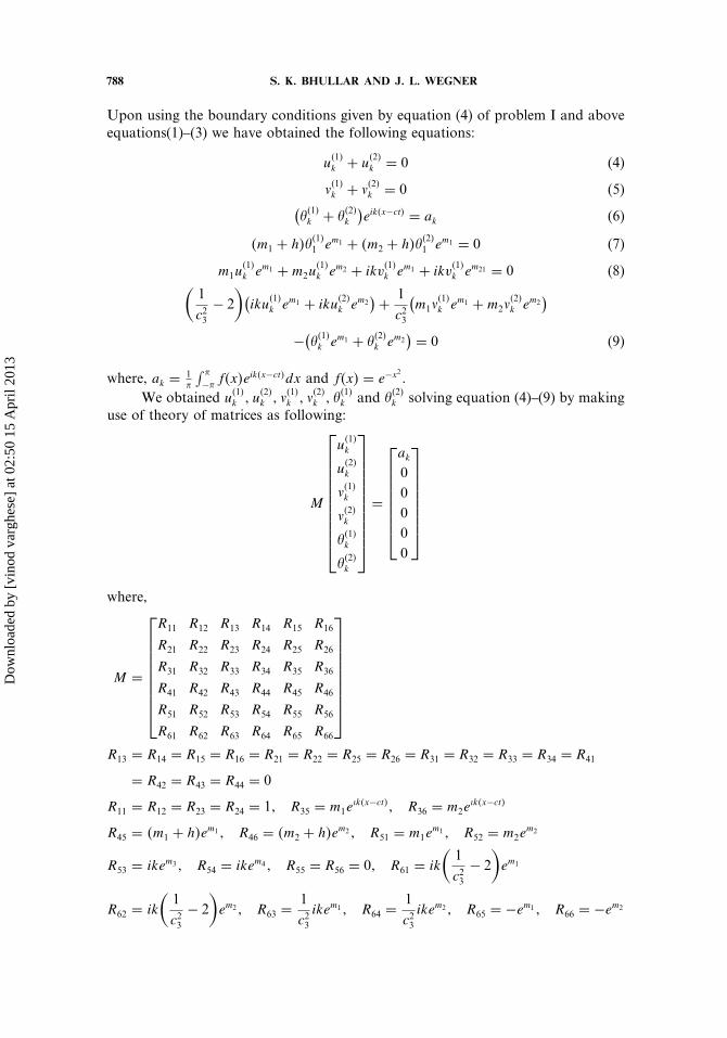
Upon using the boundary conditions given by equation (4) of problem I and aboveequations(1)–(3) we have obtained the following equations:

u�1�k + u

�2�k = 0 (4)

��1�k + �

�2�k = 0 (5)(

��1�k + �

�2�k

)eik�x−ct� = ak (6)

�m1 + h��1�1 em1 + �m2 + h��

�2�1 em1 = 0 (7)

m1u�1�k em1 +m2u

�1�k em2 + ikv

�1�k em1 + ikv

�1�k em21 = 0 (8)(

1

c23− 2

)(iku

�1�k em1 + iku

�2�k em2

)+ 1

c23

(m1�

�1�k em1 +m2�

�2�k em2

)

−(��1�k em1 + �

�2�k em2

) = 0 (9)

where, ak = 1�

∫ �

−�f�x�eik�x−ct�dx and f�x� = e−x2 .

We obtained u�1�k � u

�2�k � �

�1�k � �

�2�k � �

�1�k and �

�2�k solving equation (4)–(9) by making

use of theory of matrices as following:

M

u�1�k

u�2�k

��1�k

��2�k

��1�k

��2�k

=

ak

00000

where,

M =

R11 R12 R13 R14 R15 R16

R21 R22 R23 R24 R25 R26

R31 R32 R33 R34 R35 R36

R41 R42 R43 R44 R45 R46

R51 R52 R53 R54 R55 R56

R61 R62 R63 R64 R65 R66

R13 = R14 = R15 = R16 = R21 = R22 = R25 = R26 = R31 = R32 = R33 = R34 = R41

= R42 = R43 = R44 = 0

R11 = R12 = R23 = R24 = 1� R35 = m1e�k�x−ct�� R36 = m2e

�k�x−ct�

R45 = �m1 + h�em1� R46 = �m2 + h�em2� R51 = m1em1� R52 = m2e

m2

R53 = ikem3� R54 = ikem4� R55 = R56 = 0� R61 = ik

(1

c23− 2

)em1

R62 = ik

(1

c23− 2

)em2� R63 =

1

c23ikem1� R64 =

1

c23ikem2� R65 = −em1� R66 = −em2

Dow

nloa

ded

by [

vino

d va

rghe

se]

at 0

2:50

15

Apr

il 20

13


Therefore,

u�1�k

u�2�k

��1�k

��2�k

��1�k

��2�k

= M−1

ak

00000

APPENDIX II

To determine A1j� A2j� A3j� A4j �j = 1� 2� � � � � N − 1�, we are making use ofboundary conditions given by equation (45) along with the equations (48)–(50).These equations are containing A1j� A2j� A3j� A4j� A1j+1� A2j+1� A3j+1� A4j+1 and inmatrix form these equations can be written as:

Pj

A1j+1

A2j+1

A3j+1

A4j+1

= Qj

A1j

A2j

A3j

A4j

which further givesA1j+1

A2j+1

A3j+1

A4j+1

= P−1

j Qj

A1j

A2j

A3j

A4j

where

Pj =

cosh �j+1x sinh �j+1x cosh j+1x sinh j+1x

Kj+1�j+1 sinh �j+1x Kj+1�j+1 cosh �j+1x Kj+1j+1 sinh �j+1x Kj+1j+1 cosh j+1x

rj+1 cosh �j+1x −rj+1 sinh �j+1x pj+1 cosh j+1x −pj+1 sinh j+1x

j+1rj+1E1 − j+1rj+1E2 j+1pj+1E3 − j+1pj+1E4

Qj =

cosh �jx sinh �jx cosh jx sinh jx

Kj�j sinh �jx Kj�j cosh �1x Kjj sinh �jx Kjj cosh jx

rj cosh �jx −rj sinh �jx pj cosh jx −pj sinh jx

jrjE′1 − jrjE

′2 jpjE

′3 − jpjE

′4

E1 = �j+1 sinh �j+1x − �j+1 cosh �j+1x� E2 = −�j+1 cosh �j+1x − �j+1 sinh �j+1x

E3 = j+1 sinh j+1x − �j+1 cosh j+1x� E4 = −j+1 cosh j+1x − �j+1 sinh j+1x

E′1 = �j sinh �jx − �j cosh �jx� E′

2 = −�j cosh �jx − �j sinh �jx

E′3 = j sinh jx − �j cosh jx� E′

4 = −j cosh jx − �j sinh jx� j =j + 2�j

1 + 2�1

Dow

nloa

ded

by [

vino

d va

rghe

se]

at 0

2:50

15

Apr

il 20

13


Successive use of this relation gives:

A1N

A2N

A3N

A4N

= P−1

N−1QN−1 · · ·P−11 Q1

A11

A21

A31

A41

(10)

Now equation (10) along with boundary conditions given by equation (44) and (46)of problem II, gives

A1N

A2N

A3N

A4N

= �Fjk��Ejk�

−1

HA�As

−1

0HB�Bs

−1

0

where,

�Fjk� = P−1N−1QN−1 � � � P

−11 Q and �Ejk� is matrix with elements �

E11 = �1 sinh �1x0 −HA cosh �1x0� E12 = �1 cosh �1x0 −HA sinh �1x0�

E13 = 1 sinh 1x0 −HA cosh 1x0� E14 = 1 cosh 1x0 −HA sinh 1x0�

E21 = ��1r1 − �1� cosh �1x0� E22 = ��1r1 − �1� sinh �1x0�

E23 = �1p1 − �1� cosh 1x0� E24 = �1p1 − �1� sinh 1x0�

E31 = �1 sinh �1x1 +HB cosh �1x1� E32 = �1 cosh �1x1 +HB sinh �1x1

E33 = 1 sinh 1x1 +HB cosh 1x1� E34 = 1 cosh 1x1 +HB sinh 1x1

E41 = ��1r1 − �1� cosh �1x1� E42 = ��1r1 − �1� sinh �1x1

E43 = �1p1 − �1� cosh 1x1� E44 = �1p1 − �1� sinh 1x1

For �j�x� t�� uj�x� t�, and �j�x� t�, we have following expressions

�j�x� t� =12i�

∫ �+i�

�−i��je

stds� uj�x� t� =12i�

∫ �+i�

�−i�uje

stds

and �j�x� t� =12i�

∫ �+i�

�−i��je

stds

Dow

nloa

ded

by [

vino

d va

rghe

se]

at 0

2:50

15

Apr

il 20

13

Documents

01495730903018499