UNIVERSITY OF CALIFORNIA, SAN DIEGO

Arctic Ocean Long-Term Acoustic Monitoring: Ambient Noise, Environmental Correlates, and Transients North of Barrow, Alaska

A Thesis submitted in partial satisfaction of the requirements for the degree Master of Science

in

Engineering Science (Applied Ocean Sciences)

by

Ethan H Roth

Committee in charge:

Professor John Hildebrand, Chair Professor Carl Gibson Professor Stefan Llewellyn Smith

2008

Copyright

Ethan H Roth, 2008

All rights reserved.

iii

The Thesis of Ethan H Roth is approved and it is acceptable in quality and form for

publication on microfilm and electronically:

_____________________________________________________________________

_____________________________________________________________________

_____________________________________________________________________ Chair

University of California, San Diego

2008

iv

This thesis is dedicated to Donald Ross

for his mentorship, guidance, and friendship.

v

“Our culture, the very deepest part of our being, rises or falls with the fate of the whales and seals and other species in Arctic waters. The ancient values that define us as a people are transmitted through participation in traditional whaling and hunting

activities. If we lose the hunt, we lose our identity. It's that simple.”

Edward Itta, North Slope Borough Mayor & Inupiat Whaling Captain

vi

TABLE OF CONTENTS

Signature Page…………………………………………..………………….…

Dedication………………………………………………………………..……

Epigraph……………………………………………………………................

Table of Contents…………………………………………………….…….....

List of Figures………….…………………………………………………...…

Acknowledgements………………………………………………….…….….

Abstract……………………………………………………………..………...

I. Introduction……………………………………………………………...….

Current State of the Arctic Ocean…………………………………….

Arctic Ambient Noise…………………………………………………

Acoustic Monitoring from the Seafloor……………………………….

Baseline Study………………………………………………………...

II. Methods……………………………………………………………….……

HARP Instrumentation………………………………………………..

Field Work & Data Collection………………………………………..

Hydrophone Calibration………………………………………………

Digital Signal Processing with MatLab………………………………

Spectral Averaging……………………………………………………

Electronic & System Noise…………………………………………...

AMSR-E Sea Ice Concentration Data………………………………...

Barrow Wind Speed Data……………………………………………..

Sound Speed Profiles………………………………………………….

iii

iv

v

vi

viii

xii

xiii

1

1

3

7

11

15

15

20

24

28

31

35

38

42

43

vii

III. Results…………………………………………………………………….

Ambient Noise Measurements………………………………………..

Environmental Correlates……………………………………………..

IV. Analysis…………………………………………………………………...

Man-Made Seismic & Low-Frequency Noise………………………...

Microseisms & Earthquakes…………………………………………..

Transient Sea Ice Events……………………………………………....

Wind-Driven Noise…………………………………………………...

Bioacoustic Detections………………………………………………..

V. Discussion…………………………………………………………………

Arctic Sound Propagation…………………………………………….

Ambient Noise Level Distributions…………………………………..

Sea Ice Kinematics…………………………………………………....

Shifts in Sea Ice & Waveguide Propagation …………………………

The Marginal Ice Zone………………………………………………..

Contribution of Noise-Generating Mechanisms………………………

Statistical Density Distributions………………………………………

Implications for Arctic Marine Mammal Research…………………...

VI. Conclusion………………………………………………………………..

References…………………………………………………………………

46

46

57

60

60

62

64

66

69

76

76

78

80

83

85

87

88

91

94

96

viii

LIST OF FIGURES

Figure 1.1 – A comparison between the average sea ice extent for September

2007 and September 2005…………………………………………………….

Figure 1.2 – Typical sound-pressure levels of open ocean ambient noise, as

measured by Wenz (1962).…………………………………………………...

Figure 1.3 – Typical ray diagram and corresponding sound-speed profile for

acoustic propagation in the Arctic Ocean…………………………………….

Figure 1.4 – Study Area: shallow vs. deep ocean acoustics……………….....

Figure 1.5 – Spherical vs. Cylindrical Spreading…………………………….

Figure 1.6 – Propagation Model with shallow source and open water surface

layer.…………………………………………………………………………..

Figure 1.7 – Propagation Model with shallow source and ice-covered

surface layer…………………………………………………………………..

Figure 1.8 – Propagation Model with deep source and ice-covered surface

layer…………………………………………………………………………...

Figure 2.1 – The hydrophone sensor components……………………………

Figure 2.2 – The datalogger components……………………………………..

Figure 2.3 – The seafloor package components………………………………

Figure 2.4 – HARP instrument locations……………………………………..

Figure 2.5 – After the ballast weight is released, the HARP floats to the

surface and is recovered aboard the Healy…………………………………...

Figure 2.6 – An aerial view of the U.S. Navy’s Transducer Calibration

Center……………………………………........................................................

Figure 2.7 – Geometry of source and receiver in a calibration station……….

Figure 2.8 – Orienting a line hydrophone in a calibration station……………

Figure 2.9 – The shape of the hydrophone sensitivity used in this study is

determined by the transducer and pre-amplifier circuit………………………

Figure 2.10 – The transfer function is applied to the data in order to correct

for hydrophone sensitivity……………………………………………………

1

5

6

7

8

9

10

11

16

18

20

21

23

24

25

26

27

28

ix

Figure 2.11 – Long-term spectral averages show when acoustics events

occur in the time series……………………………………………………….

Figure 2.12 – Probability density function of the mean square (left) and

logarithm (right)………………………………………………………………

Figure 2.13 – Mean and standard deviation of noise level modeled by l

tones, with 2ln the received noise power……………………………………..

Figure 2.14 – Digital synthesis of the FIFO noise – sixteen amplitude-spikes

occurring every 4000 samples in the data…………………………………….

Figure 2.15 – Spectrogram of hard drive noise during spin-up and disk

write, occurring approximately every 8 minutes in the data………………….

Figure 2.16 – The noise floor curve was empirically determined for the

high-frequency band from flat values in the spectral time series…………….

Figure 2.17 – An example of a daily-average of AMSR-E sea ice

concentration data, viewed at a 4x4 km linear-pixel projection in WIM…….

Figure 2.18 – Mask areas used to perform time series analysis on AMSR-E

sea ice concentration data…………………………………………………….

Figure 2.19 – Vertical depth profiles for water temperature (left) and sound

speed (right) were measured by XBT probes during the summer of 2007.......

Figure 3.1 – Low-frequency background levels for sites A (Sep. 06 – Jan.

07) and B (Sep. 06 – May 07) during the duration of HARP deployment and

successful data recording..................................................................................

Figure 3.2 – High-frequency background levels for sites A (Sep. 06 – Jan.

07) and B (Sep. 06 – May 07) during the duration of HARP deployment and

successful data recording..................................................................................

Figure 3.3– Site B Low-Freq. Noise Distributions...........................................

Figure 3.4– Site A Low-Freq. Noise Distributions...........................................

Figure 3.5– Site B High-Freq. Noise Distributions..........................................

Figure 3.6– Site A High-Freq. Noise Distributions..........................................

32

34

35

36

37

38

40

41

44

47

49

50

52

54

56

x

Figure 3.7– Time series of sound-pressure spectrum levels for three different

frequencies (25, 100, 5000 Hz) plotted with daily-average wind speed

values over Barrow, as well as the percentage of sea ice coverage for a

specified area (10, 40, 100 nautical mile radius) centered around the

instrument sites.................................................................................................

Figure 4.1 – Time scales of noise-generating mechanisms..............................

Figure 4.2 – Modal dispersion of airgun shots from a seismic oil exploration

survey, as received by the HARP hydrophone on the seafloor.........................

Figure 4.3 – Tonals like these have the acoustic signature of recipricating

machinery..........................................................................................................

Figure 4.4 – Pressure spectra from the Pacific, Atlantic, and Arctic seafloor..

Figure 4.5 – Pressure ridging caused by interactions between adjacent ice

floes...................................................................................................................

Figure 4.6 – Thermal fracturing due to atmospheric cooling...........................

Figure 4.7 – Storm-generated winds produce noise related to snow blowing

over ice or leads opening..................................................................................

Figure 4.8 – The influence of wind-driven surface wave noise is only

apparent in open ocean conditions above 7 kts.................................................

Figure 4.9 – Bowhead whale call detections…………………………………

Figure 4.10 – Beluga whale call detections......................................................

Figure 4.11 – Bearded seal call detections........................................................

Figure 4.12 – Representative spectrogram of a commonly encountered

ringed seal calling sequence..............................................................................

Figure 4.13 – Spectrogram showing a rapid series of walrus knocks...............

Figure 5.1 – Transmission loss measurements versus range in the Arctic

Ocean for various frequencies………………………………………………..

Figure 5.2 – Ray paths from sources at the surface propagate directly to a

bottom-mounted hydrophone…………………………………………………

Figure 5.3 – An acoustic plane wave reflected from a random distribution of

elliptical half-cylinders……………………………………………………….

58

60

61

62

63

64

66

67

68

70

72

74

75

75

76

77

78

xi

Figure 5.4 – Sea ice kinematics………………………………………………

Figure 5.5 – Variations in ambient noise spectrum levels for frequencies of

100, 315, and 1000 Hz………………………………………………………..

Figure 5.6 – Composite of ambient noise observed in April 1982 at the Fram

IV ice camp…………………………………………………………………...

Figure 5.7 – Power spectrum levels in third-octave bands of three ambient

noise samples…………………………………………………………………

81

87

89

90

xii

ACKNOWLEDGEMENTS

I would like to acknowledge John Hildebrand for his support as my graduate

advisor, and Sean Wiggins for his guidance over the past few years. The SIO Whale

Acoustics Lab has been an amazing learning environment because of the people

comprised within it. Beve Kennedy especially helped to make this work possible.

I couldn’t ask for a better mentor than Don Ross, or a better friend than Josh

Jones.

I would like to thank Robert Small, from the Alaska Department of Fish &

Game, for his support and sponsorship of this project. Hopefully the work we’ve

started will continue to grow with our endeavor to observe and understand the changes

taking place in the Arctic.

Thanks to Caryn Rea from Conoco-Phillips, for her logistical support that

made the 2006 instrument deployment possible. Thanks to Larry Mayer from CCOM-

UNH, for his generous logistical support that made the 2007 recovery and

redeployment possible, and soon to be the same in 2008.

I’d like to especially acknowledge the crew members of the USCGC Healy and

M/V Torsvik, for helping to make this field work possible in such an extreme and

remote environment. Thanks to the Barrow Arctic Science Consortium for providing

shelter, food, and good company on land.

I would like to thank Mati Kahru for helping me obtain sea ice satellite data to

work with in his software package, Windows Image Manager.

xiii

ABSTRACT OF THE THESIS

Arctic Ocean Long-Term Acoustic Monitoring:

Ambient Noise, Environmental Correlates, and Transients North of Barrow, Alaska

by

Ethan H Roth

Master of Science in Engineering Science (Applied Ocean Sciences)

University of California, San Diego, 2008

Professor John Hildebrand, Chair

The Arctic Ocean has experienced wide-spread decreases in sea ice

concentrations that may impact various marine ecosystems. This study analyzes

yearlong ocean acoustic recordings from north of Barrow, Alaska, to provide baseline

measurements prior to possible increases in anthropogenic activities. In September

2006, two autonomous High-frequency Acoustic Recording Packages (HARPs) were

deployed to the seafloor (250m), where sound was continuously recorded by

xiv

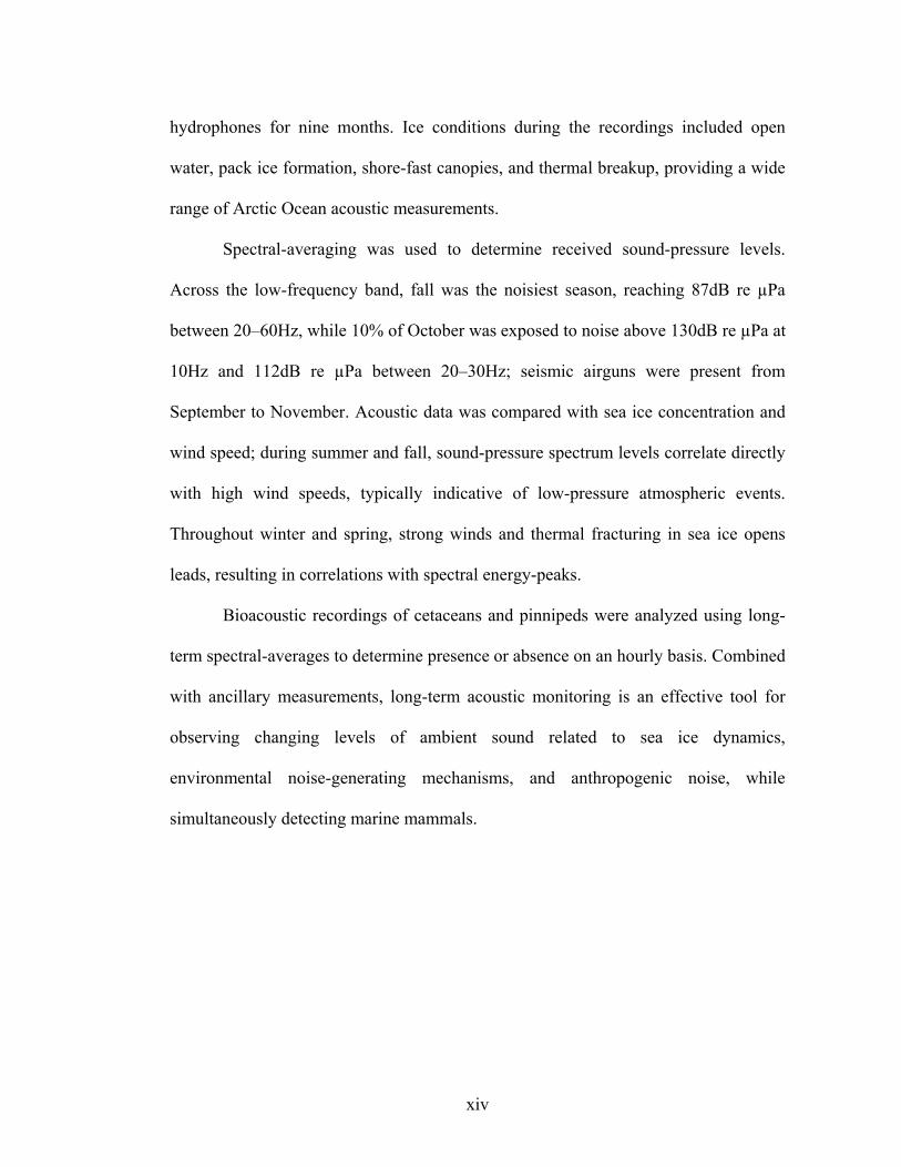
hydrophones for nine months. Ice conditions during the recordings included open

water, pack ice formation, shore-fast canopies, and thermal breakup, providing a wide

range of Arctic Ocean acoustic measurements.

Spectral-averaging was used to determine received sound-pressure levels.

Across the low-frequency band, fall was the noisiest season, reaching 87dB re µPa

between 20–60Hz, while 10% of October was exposed to noise above 130dB re µPa at

10Hz and 112dB re µPa between 20–30Hz; seismic airguns were present from

September to November. Acoustic data was compared with sea ice concentration and

wind speed; during summer and fall, sound-pressure spectrum levels correlate directly

with high wind speeds, typically indicative of low-pressure atmospheric events.

Throughout winter and spring, strong winds and thermal fracturing in sea ice opens

leads, resulting in correlations with spectral energy-peaks.

Bioacoustic recordings of cetaceans and pinnipeds were analyzed using long-

term spectral-averages to determine presence or absence on an hourly basis. Combined

with ancillary measurements, long-term acoustic monitoring is an effective tool for

observing changing levels of ambient sound related to sea ice dynamics,

environmental noise-generating mechanisms, and anthropogenic noise, while

simultaneously detecting marine mammals.

1

I. INTRODUCTION

Current State of the Arctic Ocean

The summer of 2007 set a new record low for Arctic sea ice extent (see Figure

1.1), leaving the environment on the verge of a fundamental shift towards seasonal ice

cover, which may be realized as early as 2030 (Stroeve et al, 2007). Multiyear ice has

been disappearing and being replaced by newly formed frail and thin seasonal ice that

is more easily disturbed by low-pressure winds and warmer sea temperatures.

Recently, some 965,300 square miles of perennial ice have been lost — a 50%

decrease between Feb. 2007 and Feb. 2008 (Meier quoted by Kaufman, 2008).

Figure 1.1 – A comparison between the average sea ice extent for September 2007 and September 2005; the magenta line indicates the long-term median from 1979 to 2000. September 2007 sea ice extent was 4.28 million square kilometers (1.65 million square miles), compared to 5.57 million square kilometers (2.14 million square miles) in September 2005. This image is from the NSIDC Sea Ice Index. Computer models suggest Arctic sea ice is a sensitive climate indicator,

demonstrating how the rise in global temperatures may accelerate further reductions in

2

ice cover. An important factor that has contributed to sea ice extent minimums in

recent years is the weakened and thinner state of spring ice, which takes less thermal

energy to melt than thick multiyear ice. Another factor that was particularly significant

during the summer of 2007 was an unusual atmospheric pattern, with persistent high

atmospheric pressures over the central Arctic Ocean and lower pressures over Siberia.

Clear skies under the high-pressure cell and wind patterns pumping warm air into the

region promoted strong melt while pushing ice away from the Siberian shore (Stroeve

et al, 2007).

For the first time in human-recorded history, the Northwest Passage was

completely open, bolstering the vision for a shorter sea route between the Pacific and

Atlantic Oceans. On the other hand, the Northern Sea Route along the Eurasian coast

was completely blocked by a band of ice. As the Arctic system continues to warm,

spring melt will come earlier and fall ice formation will begin later, extending the

length of the summer melt season. This has already begun to affect native subsistence

hunting, made traveling across tundra difficult, and buildings on permafrost unsafe.

The recent widespread decreases in sea ice concentrations may severely impact

marine ecosystems, which makes it imperative to establish baseline acoustic

measurements for ambient noise levels in the Arctic underwater environment prior to

possible increases in Arctic anthropogenic activities. By initiating a study across large

temporal scales, it’s possible to determine the sources of sound that are attributed to

different seasonal variations. Long-term acoustic monitoring can help to fully

understand these changes, as year-long data collection exploits the seasonal variability

3

of sea ice in a specific region. Local contributions to the soundscape include sea ice,

wind, biological vocalizations, and anthropogenic sources of noise such as seismic oil

exploration and shipping activities. To fully understand the unique noise-generating

mechanisms inherent to the Arctic Ocean environment, it’s useful to examine what

past studies have been conducted.

Underwater acoustics in the Arctic Ocean was given a great deal of attention

during the Cold War due to the fear of submarine warfare in the circumpolar north.

Sonar detection algorithms used in open ocean conditions were not well adapted to

deal with the highly-impulsive, non-Gaussian nature of ambient noise distinct to an

ice-covered environment. The role of a dynamic sea ice boundary in dictating the

seasonal variation of acoustic propagation was poorly understood. Several

acousticians carried out field experiments to identify and describe the transient sources

of noise generation that correspond with the different spatial and temporal

characteristics of sea ice. In addition, a great deal of theoretical work focused on

propagation modeling to understand the effects that under-ice scattering strength and

reflection loss had on sound transmission. It was found that the physical mechanisms

attributed to sea ice dynamics serve as both the principal control of sound propagation

over long ranges, as well as the dominant noise source in the local region.

Arctic Ambient Noise

Underwater ambient noise is described as the composite noise arising from all

sources in the sea (Kibblewhite and Jones, 1976) as well as processes occurring at or

4

above the sea surface. Urick identified surface waves, rain, biological activity, oceanic

turbulence, shipping and other anthropogenic noise, seismic disturbances, thermal

noise, and most significantly the hydrostatic effects of tides and waves as sources of

ambient noise in the deep ocean (see Figure 1.2). When introducing sea ice as an

upper boundary layer, it is the sea ice itself that governs underwater ambient noise

levels. While the sources described by Urick are still present, ice cover on the surface

can effectively inhibit these mechanisms from contributing to underwater noise,

especially the generation of wind-driven surface waves. On the other hand, sea ice acts

as an interface between the atmosphere and ocean, inducing noise through perpetual

mechanical changes that are influenced by variations in temperature and wind speed.

For this reason, sea ice is also a significant noise source and at high frequencies

contributes to excess noise above the thermal noise threshold (Kibblewhite and Jones,

1976).

5

Figure 1.2 – Typical sound-pressure levels of open ocean ambient noise, as measured by Wenz (1962). Reprinted from the National Research Council, 2003 – Ocean Noise and Marine Mammals. The Arctic waveguide is typically defined by a nearly isothermal water

column, an ice canopy at the sea surface that is spatially and temporally variable, and a

positive sound speed gradient. Acoustic ray paths are usually refracted upwards and

subsequently reflected and scattered from the rough underside of sea ice, as illustrated

in Figure 1.3. Even low-frequency (10-100 Hz) transmission loss is more substantial

than most free-surface scattering theories since acoustic waves interfere regularly due

6

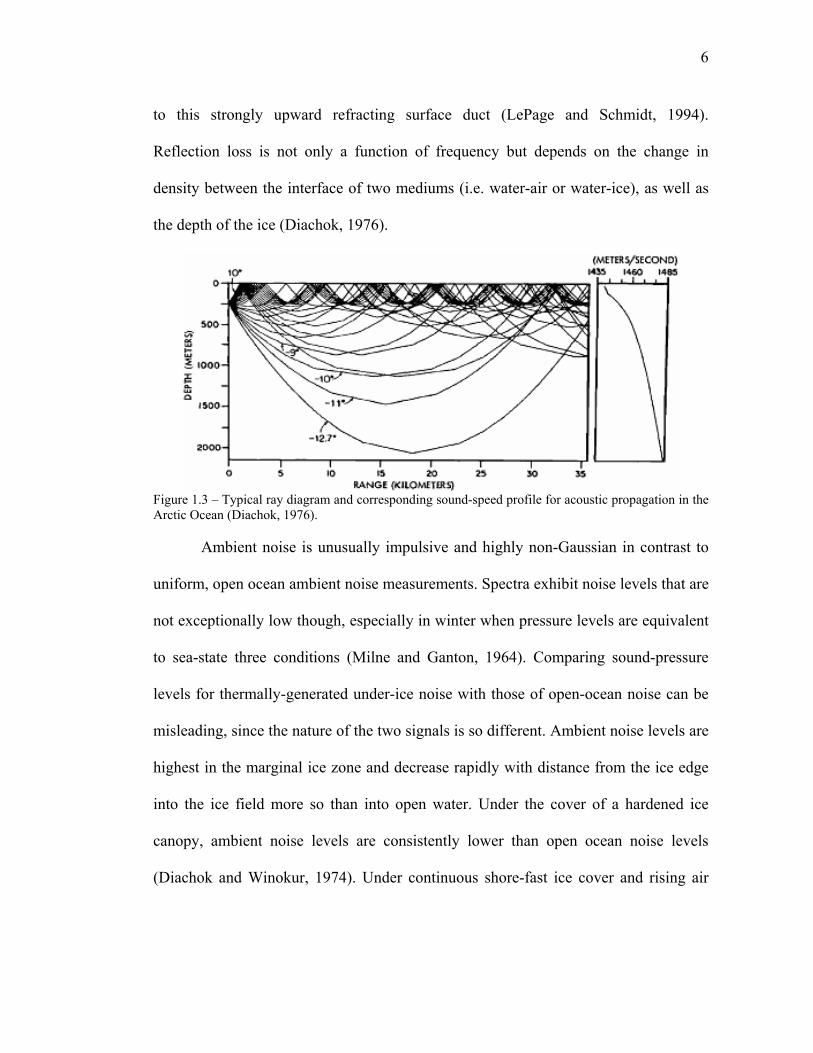
to this strongly upward refracting surface duct (LePage and Schmidt, 1994).

Reflection loss is not only a function of frequency but depends on the change in

density between the interface of two mediums (i.e. water-air or water-ice), as well as

the depth of the ice (Diachok, 1976).

Figure 1.3 – Typical ray diagram and corresponding sound-speed profile for acoustic propagation in the Arctic Ocean (Diachok, 1976). Ambient noise is unusually impulsive and highly non-Gaussian in contrast to

uniform, open ocean ambient noise measurements. Spectra exhibit noise levels that are

not exceptionally low though, especially in winter when pressure levels are equivalent

to sea-state three conditions (Milne and Ganton, 1964). Comparing sound-pressure

levels for thermally-generated under-ice noise with those of open-ocean noise can be

misleading, since the nature of the two signals is so different. Ambient noise levels are

highest in the marginal ice zone and decrease rapidly with distance from the ice edge

into the ice field more so than into open water. Under the cover of a hardened ice

canopy, ambient noise levels are consistently lower than open ocean noise levels

(Diachok and Winokur, 1974). Under continuous shore-fast ice cover and rising air

7

temperatures, noise levels between 10-1000 Hz can be up to 25 dB below those

observed for sea state zero in the open ocean (Kibblewhite and Jones, 1976).

Acoustic Monitoring from the Seafloor

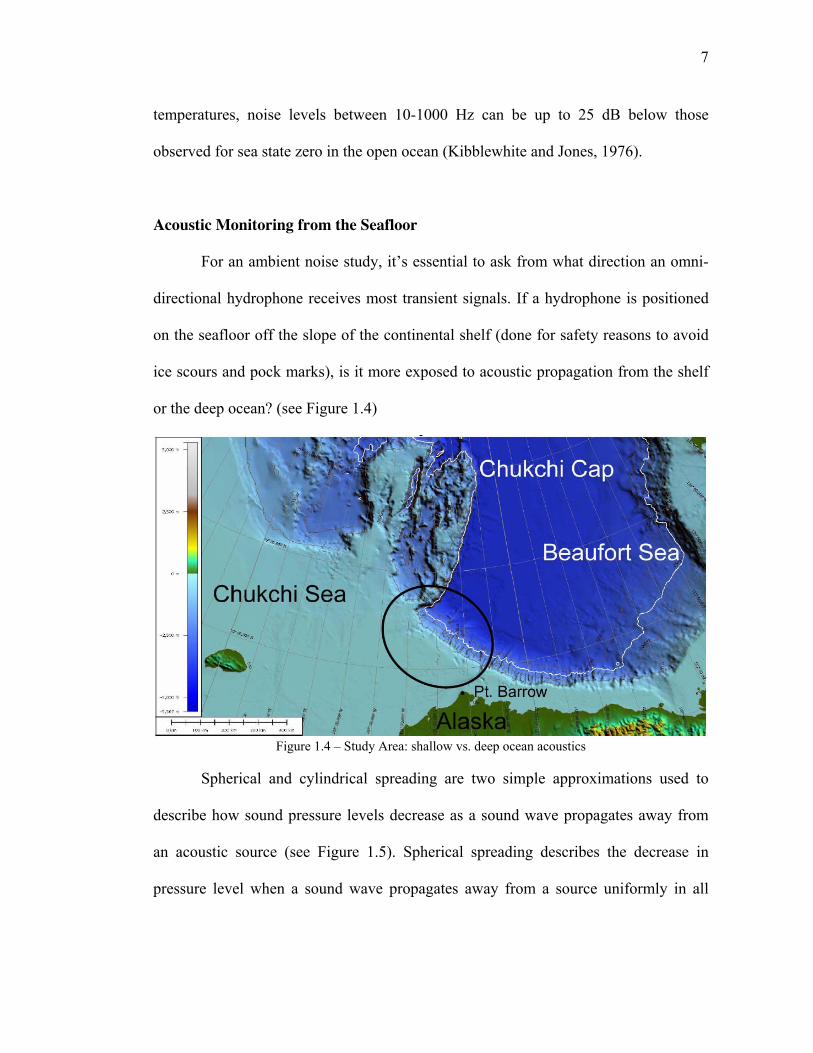
For an ambient noise study, it’s essential to ask from what direction an omni-

directional hydrophone receives most transient signals. If a hydrophone is positioned

on the seafloor off the slope of the continental shelf (done for safety reasons to avoid

ice scours and pock marks), is it more exposed to acoustic propagation from the shelf

or the deep ocean? (see Figure 1.4)

Figure 1.4 – Study Area: shallow vs. deep ocean acoustics

Spherical and cylindrical spreading are two simple approximations used to

describe how sound pressure levels decrease as a sound wave propagates away from

an acoustic source (see Figure 1.5). Spherical spreading describes the decrease in

pressure level when a sound wave propagates away from a source uniformly in all

8

directions. This situation occurs for an acoustic source at mid-depth in the deep ocean,

and the magnitude of intensity decreases as the inverse square of the range. Beyond

some range the acoustic wave eventually hits the sea surface or sea floor. A simple

approximation for spreading loss in a medium with upper and lower boundaries can be

obtained by assuming the sound is distributed uniformly over the surface of a cylinder.

Figure 1.5 – Spherical vs. Cylindrical Spreading

In the ice-covered Arctic, transmission loss is much greater than cylindrical

spreading. Due to the surface duct formed by a shallow thermal gradient, sound waves

tend to refract off the duct and propagate towards the surface, which then reflect off

the underside of rough ice, characteristic of high scattering strength. Therefore sound

will attenuate rapidly the more it reflects off the ice, and as frequency increases so

does reflection loss and surface scattering. This suggests high frequency sound cannot

travel across long distances and the hydrophone is mostly receiving locally produced

noise at high frequencies. Reflection and transmission coefficients are generally

1020 log ( )TL r dB= 1010 log ( )TL r dB=

9

proportional to the thickness of sea ice, and as a result determine the frequency-

dependent shape of the ambient noise spectrum (Diachok & Winokur, 1974).

As a theoretical exercise, several models were developed using the underwater

acoustic propagation modeling software AcTUP V2.2L (A. Maggi and A. Duncan,

Curtin University of Technology) in MatLab. Since the goal is to replicate the

continental shelf sloping down to abyssal bathymetry, the RAMGeo algorithm was

used because it provides a fully range dependent parabolic equation code for a fluid

seabed. Figure 1.6 is a model simulation with an open water upper boundary. The

shallow water source at 20 meters depth is transmitting 50 Hz across a range of 30

kilometers; the receiver is positioned on the slope just off the shelf at approximately

250 meters depth. Acoustic energy propagates very well in a shallow waveguide and

channels it through the upper layer of the deep ocean.

Figure 1.6 – Propagation Model with shallow source and open water surface layer.

10

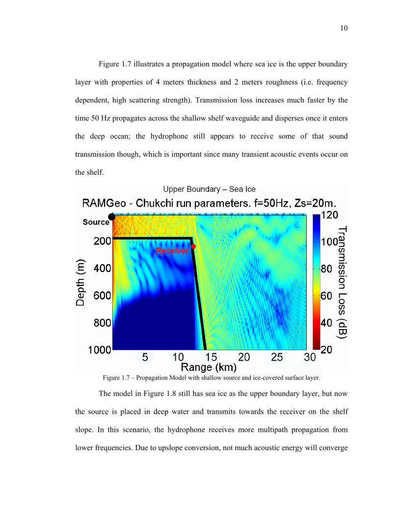
Figure 1.7 illustrates a propagation model where sea ice is the upper boundary

layer with properties of 4 meters thickness and 2 meters roughness (i.e. frequency

dependent, high scattering strength). Transmission loss increases much faster by the

time 50 Hz propagates across the shallow shelf waveguide and disperses once it enters

the deep ocean; the hydrophone still appears to receive some of that sound

transmission though, which is important since many transient acoustic events occur on

the shelf.

Figure 1.7 – Propagation Model with shallow source and ice-covered surface layer.

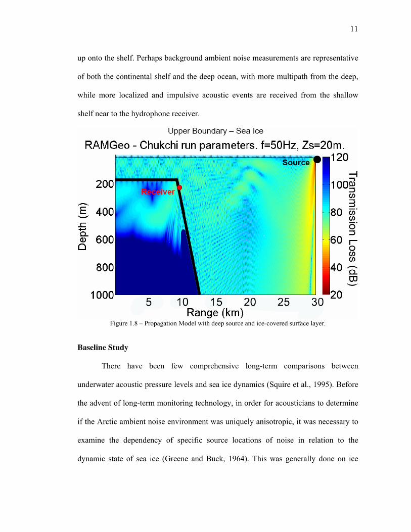
The model in Figure 1.8 still has sea ice as the upper boundary layer, but now

the source is placed in deep water and transmits towards the receiver on the shelf

slope. In this scenario, the hydrophone receives more multipath propagation from

lower frequencies. Due to upslope conversion, not much acoustic energy will converge

11

up onto the shelf. Perhaps background ambient noise measurements are representative

of both the continental shelf and the deep ocean, with more multipath from the deep,

while more localized and impulsive acoustic events are received from the shallow

shelf near to the hydrophone receiver.

Figure 1.8 – Propagation Model with deep source and ice-covered surface layer.

Baseline Study

There have been few comprehensive long-term comparisons between

underwater acoustic pressure levels and sea ice dynamics (Squire et al., 1995). Before

the advent of long-term monitoring technology, in order for acousticians to determine

if the Arctic ambient noise environment was uniquely anisotropic, it was necessary to

examine the dependency of specific source locations of noise in relation to the

dynamic state of sea ice (Greene and Buck, 1964). This was generally done on ice

12

camps while moving with the drifting floe pack, suspending hydrophones a few meters

below the ice. Milne towed hydrophones across the Beaufort seafloor at depths of 451

m; Lewis and Denner deployed an array of drifting buoys in the Beaufort Sea,

providing one of the most complete records of long-term variability and spatial

coherence of low-frequency sound in the Arctic (Webb, 1992). Autonomous

monitoring from the seafloor allows one to not only understand the spatial variability,

but more importantly the temporal variability that controls the relationship between

ambient noise and sea ice. What makes a continuous dataset like this so crucial,

especially at this point in time, is the fact that since 2005 there has been extremely

pronounced declines in sea ice concentrations.

The primary objective for the first-year of this study is to establish and

characterize long-term baseline measurements for underwater ambient noise north of

Pt. Barrow, Alaska, while examining the variability and distinct mechanisms that are

inherent in the different seasons. The broader purpose of this first-year study is to have

a baseline for which to compare future data from continuing instrument deployments.

The aim is to maintain autonomous, long-term acoustic data collection at sites around

the North Slope of Alaska for the next several years, and develop an extensive time

series where inter-comparison can reveal shifts in seasonal trends. The time-variant

impact of sea ice decline due to climate change provides adequate motivation for a

long-term study of this nature. It seems plausible that the continual thinning and

disappearance of sea ice will effectively reduce transmission loss and thus alter

underwater propagation during several months that have not previously been exposed

13

to acoustic sources such as anthropogenic noise. Seismic oil exploration and increased

shipping activity may possibly contribute to significant increases in ambient noise

levels. By initiating the experiment in 2006, it will still be feasible to use future data to

help monitor possible shifts in the acoustic baseline and determine the transient sound

sources and noise-generating mechanisms associated with noise augmentation in the

underwater sound environment.

During the summer of 2006, seismic activities associated with oil exploration

and other types of man-made noise contributed significantly to low-frequency ambient

noise levels. Fall is distinctly characterized by environmental noise such as pressure

ridging associated with ice-floe interactions, in addition to storm-generated winds. The

onset of low temperatures in early winter – when the Arctic Ocean is fully covered

with shore-fast pack ice – bring about localized thermal fracture noise; the composite

of these impulsive events exhibits a near-normal Gaussian distribution. In late winter

and spring, ambient noise is characterized by fewer impulsive events, so while thermal

fracturing is still present in addition to man-made noise, the background noise

continually decreases until reaching its lowest levels in May. Analyzing the

fluctuating trends in sound-pressure spectrum levels throughout nearly an entire year

helps to understand the effects of declining sea ice concentrations in the region,

providing the groundwork to observe changes in acoustic propagation as the current

trend continues.

The methods which made this data collection possible will be described,

including details that outline the instrumentation used and subsequent field work.

14

Sensor calibration was performed since ambient noise measurements are represented

as received pressure levels. Data analysis methods included digital signal processing

and spectral averaging in MatLab, and there was additional consideration for

electronic noise issues. Spectral curves are represented as monthly averages for

background noise levels as well as statistical density distributions that include all

transient signals.

Time series analysis was performed on sea ice concentration data from the

NASA AMSR-E satellite and wind speed data from a NOAA meteorological station in

Barrow. These are compared with time series of acoustic data – analyzed at different

frequencies in spectral space – to investigate possible correlations between sound and

the dynamic underwater environment. Several cetacean and pinniped species were

recorded, including bowhead and beluga whales, ringed and bearded seals, and walrus.

Long-term spectral-averaged time series indicate the presence or absence of three

species on an hourly basis in addition to investigating vocal repertoires throughout

varying seasonal periods. It will be shown that combined with ancillary measurements,

long-term acoustic monitoring provides an effective tool for observing changing levels

in ambient sound related to sea ice, wind, anthropogenic noise, and can simultaneously

detect marine mammals.

15

II. METHODS

HARP Instrumentation

Two autonomous, seafloor High-frequency Acoustic Recording Packages

(HARPs) were assembled and deployed for this experiment with the goal of recording

sound for an entire year; the instrumentation was similar to that described by Wiggins

(2007). The three main categories of components that make long-term acoustic data

collection possible are the hydrophone sensor (32 kHz sampling), data-logging

system, and instrument packaging.

A passive acoustic hydrophone has been designed to be broad-band in

frequency, have high sensitivity (i.e. increased gain), and low self (i.e. system) noise.

Sensor components include two types of transducers and a pre-amplifier circuit board

housed inside a pliable polyurethane tube (!OD = 2 inches), and immersed in inert

mineral oil to match the acoustic coupling impedance of water (see Figure 2.1). In

order to achieve substantial dynamic range over such a broad range of frequencies, it’s

beneficial to split the hydrophone element into two separate channels and combine

them later. A bundle of six Benthos AQ-1 cylindrical transducers connected in series

was used for the 10-3000 Hz band and provide a total sensitivity of approximately -

187 dB re 1 Vrms/Pa with a flat response (+/- 1.5 dB). One omni-directional ITC-

1042 spherical transducer was used for the 1-16 kHz band and has a flat (+/- 2 dB)

sensitivity response of about -200 dB re 1 Vrms/Pa . As acoustic pressure waves

propagate through the transducer elements, piezoelectric crystals inside the hollow

ceramics are electrically excited by compression, and in turn emit a small analog

16

voltage signal. Treating a transducer like an electric capacitor, the voltage potential

can be measured between two wires soldered to the inside and outside of the ceramic.

Figure 2.1 – The hydrophone sensor components consist of one ITC-1042 and six Benthos AQ-1 transducers, a custom-designed pre-amplifier, and Impulse underwater connector (Wiggins, 2007). Two signals are then inputted into separate stages of the pre-amplifier (i.e.

signal conditioning) circuit board. The board must be positioned as close as possible to

the transducers to avoid creating an antenna for electronic noise. Approximately 40 dB

of gain is added to the low-frequency stage and 80 dB to the high-frequency stage.

The goal is to pre-whiten the signals so their frequency response is similar to the

reciprocal of ocean ambient noise. In general, more gain is added at higher frequencies

where ambient noise levels are lower and sound attenuation is higher (Wiggins, 2007).

High-pass filters on both stages create low-end roll offs below 30 Hz on the low-

frequency stage and below 10 kHz on the high-frequency stage. A 4-pole low-pass

(i.e. anti-aliasing) filter reduces high-frequency aliasing effects above 2 kHz for the

low-frequency stage and above 100 kHz for the high-frequency stage.

Amplified signals travel through a 10 meter underwater cable and bulkhead

connector to a differential receiver onboard the datalogger, where the two stages of the

analog sensor signal are mixed and passed through another 4-pole low-pass filter with

a -3 dB rolloff point at 16 kHz, further reducing any possible high-frequency aliasing

17

effects. The filtered signal is converted into digital data using a low-power, low-noise

Analog-to-Digital Converter from Analog Devices. The A/D circuit board provides

16-bit resolution and up to 250,000 samples/second sample rate. Also included on the

A/D card is a power supply (+5 V) for the low-power hydrophone sensor (50 mW).

The datalogger CPU card is a 32-bit, 20 MHz micro-controller from Motorola,

and runs all processes onboard the datalogger (see Figure 2.2). The CPU circuit board

contains FLASH memory for data buffering, and a RS232 transceiver for a HARP

user to communicate with and program the datalogger through a standard computer

terminal with a serial communications port. After the sensor data has been digitized,

the CPU passes the binary information to the SRAM circuit board, which consists of

32 MB for data buffering. Once 30 MB of this space has been filled, the Ethernet/IDE

card spins up a hard disk and writes the SRAM buffer into a 60,000 block binary file,

while the A/D converter continues to fill up the data buffer from the back end. Each

datalogger has 16 integrated drive electronics (IDE) laptop disk drives (2.5” form-

factor), each with 120 GB of capacity (1.92 TB total). While all the disks are arranged

in a block, each disk is addressed and powered one at a time, in sequential order; this

maintains low-power consumption in the datalogger.

18

Figure 2.2 – The datalogger components consist of a CPU, A/D converter, RAM buffer, clock card, and IDE controller for sixteen 120 GB hard drives (Wiggins, 2007). For data evaluation in the field, the Ethernet/IDE circuit board also provides

10BaseT file transfer protocol (FTP) and telnet connectivity in order to upload

individual 30 MB files from a datalogger hard disk. The fifth circuit board housed

inside the datalogger is a Clock card, populated with a temperature compensating

phase-lock circuit and a low-power Seascan clock oscillator module which provides

low, long-term clock drifts on the order of 1 part in 10-8

. Precise clocks are beneficial

when sensors are deployed in an array configuration and the measured difference in

arrival times of transient signals can be useful for various signal processing techniques

(i.e. tracking).

Both storage capacity and battery life dictate the monitoring duration and

sampling rate of a HARP (Wiggins, 2007). 1.92 TB of data storage capacity allows for

approximately one year of recording duration if sampling continuously at 32 kHz. For

this particular instrument configuration, a total of 336 D size alkaline cells (140 grams

each) are arranged into five sub-packs. Housed within a separate pressure case

19

composed of 7075 aluminum, four of the sub-packs contain 72 D cells arranged in

four layers of 18 cells. The fifth sub-pack is housed along with the electronics inside

the datalogger pressure case (6061-T6 aluminum), and contains 48 D cells arranged in

four layers of 12 cells. Each sub-pack provides 12 volts of power by assembling either

nine or six parallel strings of 8 cells in series. All the sub-packs are connected in

parallel; power is transferred from the battery pressure case housing to the datalogger

using an underwater cable and bulkhead connectors from Impulse.

From this configuration of forty-two 12 volt strings, an estimated 588 Amp-

hours were available for the deployment. It was overlooked though that operating

temperatures for depths greater than 100 meters in the Arctic Ocean reach as low as -

2° C, while environmental conditions required for alkaline batteries to operate

efficiently are rated for 0° C and above. The consistent cold temperature “drained” the

battery voltages faster than anticipated; at the same time, the hard disks required more

current draw than usual in order to “spin up” in cold temperatures. At some point

during the deployment, the batteries could no longer provide sufficient current for

digitized data to be written to the hard disks. This occurred on January 31, 2007 for

Site A, and on May 30, 2007 for Site B.

Seafloor packages are easy to deploy and recover from mid-sized research,

fishing, or merchant vessels. The frames for these seafloor packages were originally

used to deploy an older generation of Ocean Bottom Seismometers. They are

constructed of fiberglass bars fastened together into a rectangular frame with

approximate dimensions 66 in. by 32.5 in. by 40.25 in. high (see Figure 2.3), and

20

contain a compact arrangement of mounted flotation, mooring ballast, and release

system. Flotation consists of eight Benthos 17" glass spheres housed in polyethylene

hard hats, and rated to 6000 meters depth. Each sphere provides 56 pounds of

buoyancy (448 pounds total), a majority of which is necessary due to the weight of the

batteries. A two-inch thick steel plate weighing approximately 340 pounds is rigidly

fixed to the bottom of the seafloor frame by securing it to two EG&G acoustic

releases. The OBS package is also where the datalogger and battery pressure cases are

mounted, while the hydrophone sensor is tethered 10 meters above the instrument

frame to provide a quieter acoustic background than near the sea surface.

Figure 2.3 – The seafloor package components consist of glass-sphere flotation, acoustic transponder releases, and ballast weight, in addition to housing the datalogger and battery pressure cases. Field Work & Data Collection

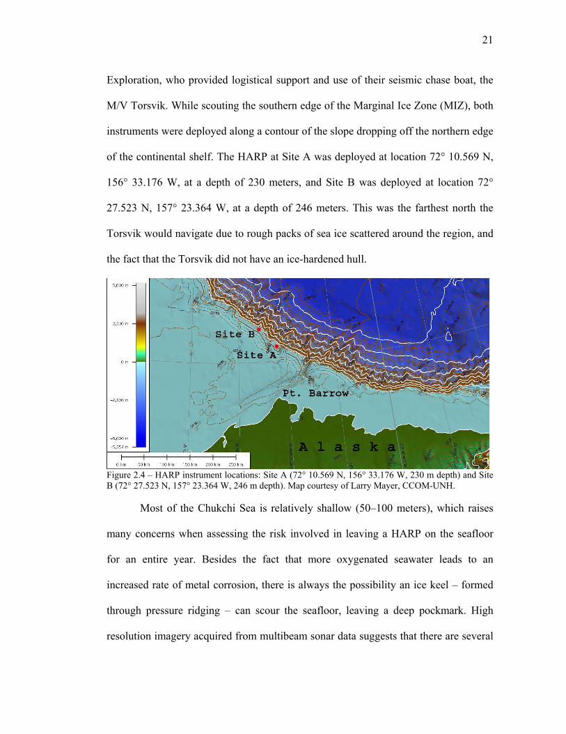
On September 25, 2006, two autonomous HARPs were deployed to the

seafloor – approximately 250 meters deep – due north of Point Barrow, Alaska in the

Chukchi Sea (see Figure 2.4). The field work effort was aided by Conoco-Phillips Oil

21

Exploration, who provided logistical support and use of their seismic chase boat, the

M/V Torsvik. While scouting the southern edge of the Marginal Ice Zone (MIZ), both

instruments were deployed along a contour of the slope dropping off the northern edge

of the continental shelf. The HARP at Site A was deployed at location 72° 10.569 N,

156° 33.176 W, at a depth of 230 meters, and Site B was deployed at location 72°

27.523 N, 157° 23.364 W, at a depth of 246 meters. This was the farthest north the

Torsvik would navigate due to rough packs of sea ice scattered around the region, and

the fact that the Torsvik did not have an ice-hardened hull.

Figure 2.4 – HARP instrument locations: Site A (72° 10.569 N, 156° 33.176 W, 230 m depth) and Site B (72° 27.523 N, 157° 23.364 W, 246 m depth). Map courtesy of Larry Mayer, CCOM-UNH. Most of the Chukchi Sea is relatively shallow (50–100 meters), which raises

many concerns when assessing the risk involved in leaving a HARP on the seafloor

for an entire year. Besides the fact that more oxygenated seawater leads to an

increased rate of metal corrosion, there is always the possibility an ice keel – formed

through pressure ridging – can scour the seafloor, leaving a deep pockmark. High

resolution imagery acquired from multibeam sonar data suggests that there are several

22

ice scours on the seafloor in the vicinity of Point Barrow. The instrument locations

were chosen to avoid these pockmarks and be on the edge of the continental shelf

drop-off so that the hydrophones would record both shallow water sound propagation

from the eastern Chukchi Sea and deep ocean (~4000 meters) acoustics from the

western Beaufort Sea.

Both HARPs were successfully recovered on August 17, 2007 aboard the

United States Coast Guard Cutter Healy, a heavy-class icebreaker used for polar

research. At each site, the ship’s 12 kHz hull transducer was used to transmit a series

of coded sonar pings to the EG&G acoustic release onboard the HARP. Measuring the

time of arrival between acoustic communications and approximating the speed of

sound allows for reasonable slant range estimation. Transmission of a final release

command triggered a solenoid firing mechanism and released the ballast weight,

allowing the positively buoyant HARP package to float up to the sea surface (see

Figure 2.5). Once sighted at the surface, a small rib boat maneuvered toward the

packages and towed them to Healy’s starboard quarter, where a crane transferred the

instruments onto the fantail deck. The HARPs were evaluated for data quality, all

necessary hardware was refurbished, and the instruments were redeployed on

September 14, 2007 for another year of autonomous recording.

23

Figure 2.5 – After the ballast weight is released, the HARP floats to the surface and is recovered aboard the Healy. During both the deployment and recovery cruises, with ice conditions

permitting, a contingent of expendable Sparton AN/SSQ-57SPC sonobuoys were

deployed to opportunistically record marine mammal vocalizations and underwater sea

ice events. Activated by a seawater battery, sonobuoy hydrophones convert

underwater sound waves into electrical signals, which are amplified and frequency

modulated for real-time VHF transmission through a radio transmitter on the surface

float to an omni-directional antenna positioned atop the vessel’s radio mast. A VHF

radio receives the signal and a PC sound card samples the acoustic data at 48 kHz. In

addition, a two-channel hydrophone – sampling at 192 kHz – was dropped into the

water on a few occasions when the vessel was stationary long enough for a sufficient

recording. This ancillary data was used only to familiarize the data analyst with Arctic

acoustics by observing transient signals and the sources that generate them.

24

Hydrophone Calibration

Calibration of the HARP hydrophone in several configurations was conducted at

the U.S. Navy’s Transducer Evaluation Center (TRANSDEC) in San Diego,

California on January 30 and April 30, 2007 (see Figure 2.6). TRANSDEC is a

transducer calibration and underwater acoustic test facility; hydrophone calibration is

ideal in this controlled environment due to low levels of ambient noise and convenient

access. The large, man-made anechoic pool is 300 ft. by 200 ft. by 38 ft. deep, and

contains 6 million gallons of chemically treated fresh water, continuously circulated to

maintain isothermal conditions.

Figure 2.6 – An aerial view of the U.S. Navy’s Transducer Calibration Center.

When making underwater sound measurements in a tank, one must consider

constructive and destructive interference from standing waves in the sound field, since

reflections off the sides, surface, and bottom of the tank are necessarily close to the

projector (i.e. source) and hydrophone (i.e. receiver). The boundary at the surface is

the most significant contributor since an air-water interface is a near perfect reflector

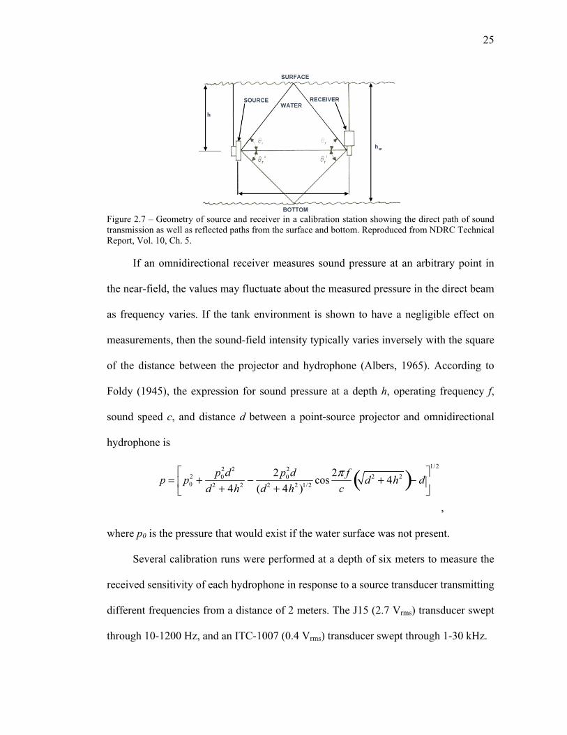
(see Figure 2.7). This makes it difficult to generate and measure a progressive plane

sound wave.

25

Figure 2.7 – Geometry of source and receiver in a calibration station showing the direct path of sound transmission as well as reflected paths from the surface and bottom. Reproduced from NDRC Technical Report, Vol. 10, Ch. 5. If an omnidirectional receiver measures sound pressure at an arbitrary point in

the near-field, the values may fluctuate about the measured pressure in the direct beam

as frequency varies. If the tank environment is shown to have a negligible effect on

measurements, then the sound-field intensity typically varies inversely with the square

of the distance between the projector and hydrophone (Albers, 1965). According to

Foldy (1945), the expression for sound pressure at a depth h, operating frequency f,

sound speed c, and distance d between a point-source projector and omnidirectional

hydrophone is

,

where p0 is the pressure that would exist if the water surface was not present.

Several calibration runs were performed at a depth of six meters to measure the

received sensitivity of each hydrophone in response to a source transducer transmitting

different frequencies from a distance of 2 meters. The J15 (2.7 Vrms) transducer swept

through 10-1200 Hz, and an ITC-1007 (0.4 Vrms) transducer swept through 1-30 kHz.

p = p02 + p0

2d 2

d 2 + 4h2 ! 2 p02d

(d 2 + 4h2 )1/2 cos2" f

cd2 + 4h2( )! d

!

"#

$

%&

1/2

26

There was also an interest in determining the directivity pattern of the

hydrophone based on the geometric arrangement of the transducer bundle. Consider

that for an omnidirectional projector, the hydrophone could receive more signals as a

result of reflected paths rather than direct path (Albers, 1965). Even at frequencies

higher than 1 kHz, the hydrophone appeared to remain omni-directional while being

rotated 180° relative to the source transducer (see Figure 2.8).

Figure 2.8 – Orienting a line hydrophone in a calibration station to minimize the effects of surface reflections. Reproduced from NDRC Technical Report, Vol. 10, Ch. 5. TRANSDEC helps to verify the expected hydrophone response based on

preamplifier measurements on the lab bench and theoretical sensitivity of the

piezoelectric transducers (see Figure 2.9). The hydrophone from Site A was replaced

during refurbishment in 2007 and brought back to San Diego, so the actual sensor used

in the first year of study was calibrated prior to data analysis. Differences between the

hydrophones at Sites A and B are expected to be less than 1 dB, due to slight

variations in hydrophone sensitivity and circuitry. The calibration testing showed the

expected response of the instrument to be within ±1-2 dB of the measured response.

27

Figure 2.9 – The shape of the hydrophone sensitivity used in this study is determined by the transducer and pre-amplifier circuit. Stage one is the low-frequency band on the left, and stage two is the high-frequency band on the right. The seafloor recorder is not expected to have a meaningful response below 10

Hz, while the high-frequency rolloff of the recorders used in the Arctic begin at 15

kHz, and provide 30 dB/octave of protection from aliasing. For the purposes of data

analysis, a transfer function can be computed based on the sensitivity of the transducer

elements in addition to the signal-conditioning provided by the pre-amplifier (see

Figure 2.10). Once subtracted from the data, this allows for spectral measurements to

be reported as absolute receive-pressure levels of ambient noise.

28

Figure 2.10 – The transfer function is applied to the data in order to correct for hydrophone sensitivity. Digital Signal Processing with MatLab

Analyzing long-term, high-frequency acoustic data is challenging due to both

the size and resolution of the time series. The “raw” binary data collected by the

HARPs is processed into 1 GB files generated in a format called XWAV; this is

similar to a WAV format but in addition contains header information such as

experimental parameters and time stamps. The data can then be spectrally analyzed

using the Signal Processing toolbox in MatLab.

Fourier analysis was performed on all data in the time-domain using the

discrete Fourier transform (DFT) to produce frequency-domain representations of the

acoustic signals. Discrete time requires that the input signal has non-zero values that

are limited or finite in duration, which is achieved through uniform sampling of the

continuous time signal. Conversion from continuous time to discrete-time samples

changes the underlying Fourier transform of x(t) into a discrete-time Fourier

29

transform, and generally includes aliasing distortion. If the Nyquist (i.e. cutoff)

frequency is known to be 16 kHz, then the appropriate sample-rate is at least twice

that value, or 32 kHz, in order to minimize aliasing effects. Similarly, transforming a

very long sequence can result in spectral leakage, which leads to a reduction in DFT

resolution; specifying an appropriate sub-sequence length, or NFFT length, is

important in minimizing such effects. A standard technique is to perform multiple

DFTs and create time-evolving spectrograms. To compute a power spectrum for data

containing noise or random processes, averaging the magnitude components of

multiple DFTs reduces the variance inherent in the spectrum.

Computationally, direct application of the DFT to a data vector of length n

requires n multiplications and n additions — a total of 2n2 floating-point operations.

Fast Fourier Transform (FFT) algorithms have computational complexity O(n log n)

instead of O(n2). For example, if n is a power of 2, a one-dimensional FFT of length n

requires less than 3n log2 n floating-point operations. For n = 220, that is a factor of

almost 35,000 faster than 2n2 (www.mathworks.com). The FFT is an efficient

algorithm to compute DFTs, and is defined by the formula

, ,

where is a primitive Nth root of unity. The complex numbers Xk represent the

amplitude and phase of the different sinusoidal components of the input signal xn.

Euler's formula helps to express sinusoids in terms of complex exponentials, which are

much easier to manipulate.

Xk = xne! 2" i

Nnk

n=0

N !1

' k = 0,K , N ! 1

e2" iN

30

Welch's method (1967), commonly referred to as the periodogram method,

estimates power spectral densities (PSD) by dividing the time signal into successive

blocks, and averaging squared-magnitude DFTs of the signal blocks. Let

, for , denote the nth block of the signal

,with N denoting the number of blocks. The Welch PSD estimate is given by

where the RHS denotes time averaging across blocks of data indexed by n. The

function ‘pwelch’ implements Welch's method in MatLab’s Signal Processing

Toolbox. Since , and since the DFT is a linear operator,

averaging magnitude-squared DFTs is equivalent to estimating block

autocorrelations , averaging them, and taking a DFT of the average. However, this

process is slower than Welch’s method.

The ‘pwelch’ function uses the Goertzel algorithm to calculate the power

spectral density by dividing the input signal vector x into k segments with no overlap.

A Hanning window is applied to each segment of x, and a 32000-point FFT is then

applied to the windowed data to obtain 1 Hz bins. The modified periodogram of each

windowed segment is computed and the set of modified periodograms is averaged to

form the spectrum estimate . The resulting spectrum estimate is scaled to

compute the power spectral density as , where the sampling frequency Fs =

32000 Hz. The number of segments k that x is divided into is calculated as /k m l= ,

xn (k) = x(k + nM ) !k = 0,1,K , M ! 1 x #C NM

!R̂x ($ k ) = 1

NDFTk (xn ) 2

n=0

N !1

' @ Xn ($ k )2{ }n

!Xn ($ k ) 2 = NgDFTk (R̂xn)

Xn ($ k ) 2

R̂xn

S(e j$ )

S(e j$ ) / Fs

31

where m is the length of the signal vector x, and l is the windowed length of each

segment.

Welch’s method returns a power spectral density estimate yielding units of

power per frequency. The units are crucial since a density can be integrated to obtain

an estimate of the average power over a given frequency interval. Moreover, Welch’s

method returns a single sided spectrum for real signals since the total power of the

signal is contained in half the spectrum (i.e. 0-16 kHz). In other words, integrating a

single-sided PSD estimate yields the average power estimate over the entire Nyquist

interval. The same result occurs if integrating a double-sided PSD estimate over the

entire sampling interval (i.e. 0-32 kHz).

Spectral Averaging

Preliminary assessment of the data was performed using Triton, GUI software

code developed in MatLab by Wiggins (2003). Long-term spectral averages (LTSAs) -

a scheme used for file compression and data overview (Wiggins, 2007) - were

computed for successive spectra by averaging 32 Hz bins over 120 sec bins throughout

the entire data set. The LTSA provides a time series of averaged-spectra arranged

sequentially, as shown in Figure 2.11. This allows the analyst to efficiently search for

and manually detect transient signals or unknown acoustic events such as marine

mammal vocalizations, sea ice mechanics, and man-made noise. Triton has built-in

functionality enabling the analyst to “zoom in” on an event in the LTSA and view its

32

spectrogram - computed directly from the XWAV file - with finer-scale resolution in

both the frequency and time axis.

Figure 2.11 – Long-term spectral averages show when acoustic events occur in the time series.

Calibrated ambient noise measurements were produced using two different

averaging schemes that pursued different analysis objectives. In both cases, 200 sec

samples of continuous data were used with no overlap between each spectral average.

All spectra were processed with a Hanning window and 32000-point FFT, yielding 1

Hz bins that provide high-resolution sound spectrums. The first method computed

monthly averages using select 200 sec samples on a near-daily basis, where no

acoustic events were observed. Of course these samples may potentially include hard-

to-detect broadband sound sources like wind or surface waves coupling with the

underwater environment. This is acceptable since the objective here is to quantify the

background noise of the underwater environment in this specific region, and provide a

conservative baseline estimate for comparison to other spectral analyses performed

throughout this study.

33

The second method computed monthly averages using continuous 200 sec

samples sequentially through the entire data set, including all transient signals and

acoustic events. Each monthly spectrum was computed continuously with 200 sec

spectrally-averaged samples, so there were approximately 17,000 spectra samples for

each month. From the statistical density distribution of these samples, ambient noise

curves were generated based on measured sound-pressure levels for the highest 1%,

upper 10%, median 50%, lower 10%, and lowest 1% of the distribution samples. The

mean curve was also computed in order to illustrate the deviation of ambient noise

level distributions from a Gaussian or Poison probability distribution.

It is important to note that all spectral averaging was performed on a

logarithmic scale rather than a linear scale. Mathematically this does not make sense,

but statistically it is logarithmic quantities that are invariably dealt with in ocean

propagation. This is because multipath propagation and scattering strength dominate

transmission fluctuations in the ocean and lead to broad statistical distributions (Dyer,

1970). It is especially the case for the Arctic Ocean, where impulsive events dominate

a sound spectrum that has ambient noise levels reported to be as much as 25 dB below

those observed for sea state zero in open ocean for the 10 - 1000 Hz frequency band

(Kibblewhite and Jones, 1976). Therefore the mean and standard deviation for any

logarithmic measure, such as acoustic transmission loss over long distances from

multiple sources, differ considerably from corresponding mean-square measures (see

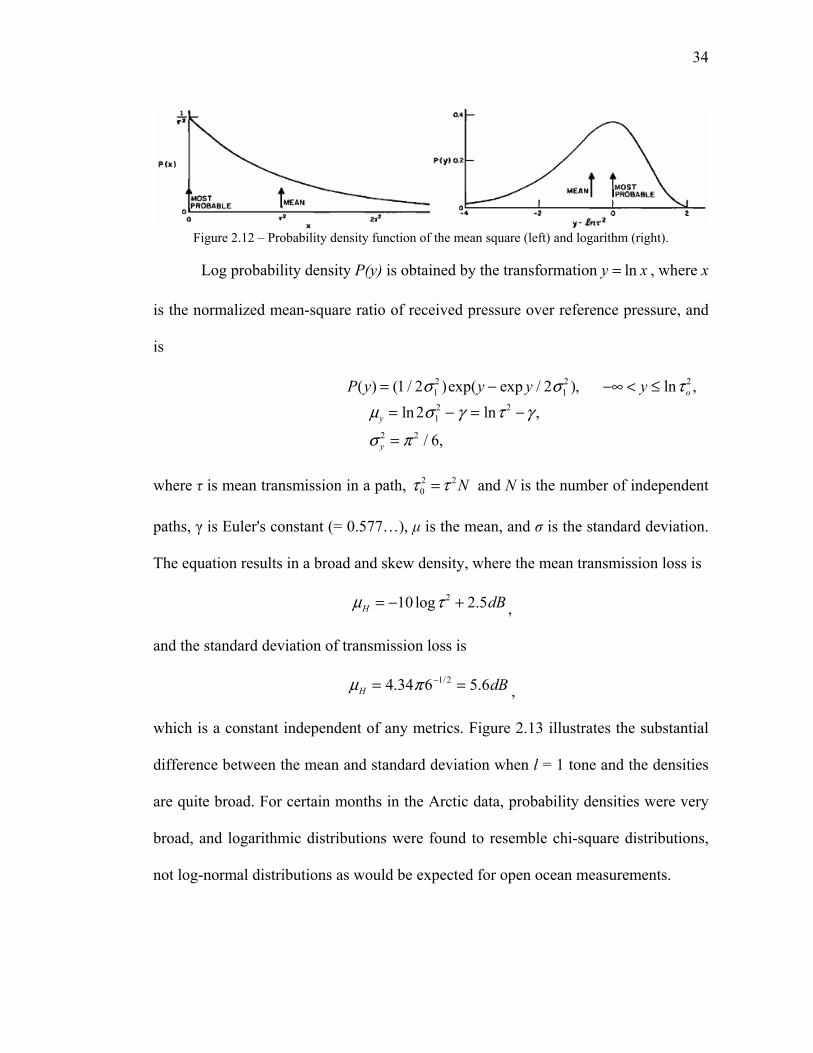
Figure 2.12) (Dyer, 1970).

34

Figure 2.12 – Probability density function of the mean square (left) and logarithm (right).

Log probability density P(y) is obtained by the transformation lny x= , where x

is the normalized mean-square ratio of received pressure over reference pressure, and

is

P(y) = (1 / 2%12 )exp(y ! exp y / 2%1

2 ), !& < y ' ln( o2 ,

µy = ln2%12 ! ) = ln( 2 !) ,

% y2 = " 2 / 6,

where " is mean transmission in a path, 2 20 N( (= and N is the number of independent

paths, ! is Euler's constant (= 0.577…), µ is the mean, and # is the standard deviation.

The equation results in a broad and skew density, where the mean transmission loss is

,

and the standard deviation of transmission loss is

,

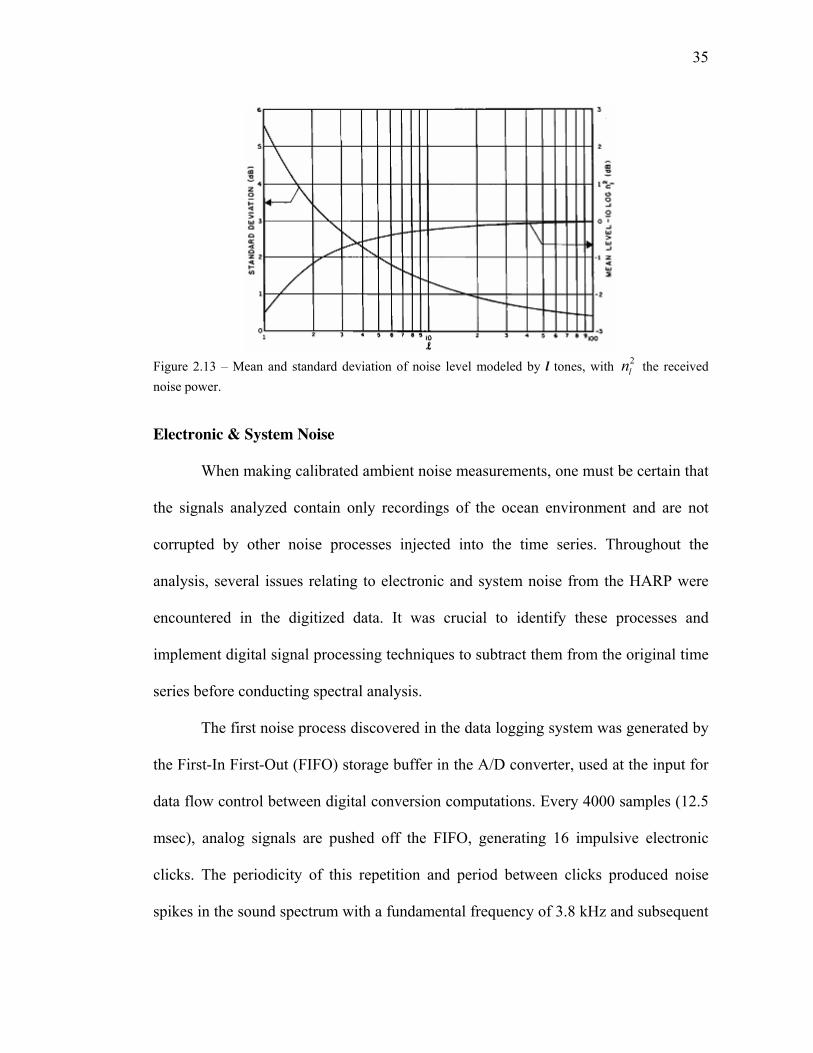
which is a constant independent of any metrics. Figure 2.13 illustrates the substantial

difference between the mean and standard deviation when l = 1 tone and the densities

are quite broad. For certain months in the Arctic data, probability densities were very

broad, and logarithmic distributions were found to resemble chi-square distributions,

not log-normal distributions as would be expected for open ocean measurements.

µH = !10 log( 2 + 2.5dB

µH = 4.34" 6!1/2 = 5.6dB

35

Figure 2.13 – Mean and standard deviation of noise level modeled by l tones, with 2

ln the received noise power. Electronic & System Noise

When making calibrated ambient noise measurements, one must be certain that

the signals analyzed contain only recordings of the ocean environment and are not

corrupted by other noise processes injected into the time series. Throughout the

analysis, several issues relating to electronic and system noise from the HARP were

encountered in the digitized data. It was crucial to identify these processes and

implement digital signal processing techniques to subtract them from the original time

series before conducting spectral analysis.

The first noise process discovered in the data logging system was generated by

the First-In First-Out (FIFO) storage buffer in the A/D converter, used at the input for

data flow control between digital conversion computations. Every 4000 samples (12.5

msec), analog signals are pushed off the FIFO, generating 16 impulsive electronic

clicks. The periodicity of this repetition and period between clicks produced noise

spikes in the sound spectrum with a fundamental frequency of 3.8 kHz and subsequent

36

harmonics at 7.6 kHz, etc. To resolve this issue, several minutes of the time series

were segmented into 4000-sample blocks, stacked on top of each other, and averaged

together; the result was a clear, isolated reproduction of the FIFO noise (see Figure

2.14). A matched filter was then generated by creating an artificial time series with the

FIFO noise repeated every 4000 samples. By subtracting the matched filter time series

from the original data time series, the FIFO noise process disappeared completely

before performing any spectral analysis.

Figure 2.14 – Digital synthesis of the FIFO noise – sixteen amplitude-spikes occurring every 4000 samples in the data. The source of the second noise process is still unknown and appears to have

fluctuated in amplitude over time. Furthermore, unlike the uniform periodicity of the

FIFO noise, this noise process evolved over time. Thus the matched filtering technique

cannot effectively subtract the noise from the data time series. While further analysis

is needed to generate the proper filter, for the purposes of this study, the noise was

dealt with in the frequency domain in order to produce “clean” spectra. Noise spikes

occurred at the fundamental frequency of 100 Hz and subsequent harmonics every 100

37

Hz across the entire frequency band. The data in these 1 Hz bins was removed and

linear interpolation was performed between the bins before and after the noise spikes.

This effectively subtracted the unknown noise process and smoothed the spectral

plots.

A third noise process originating in the datalogger is known to be hard disks

spinning up and writing for approximately one minute during every eight-minute

sampling cycle (see Figure 2.15). Again, further analysis is necessary to generate the

proper filter, but since a majority of the noise occurred within the band that is not

being reported, it was decided that the noise would remain in the time series. Note that

harmonics can be seen in the high-frequency band spectra, and should be regarded as

electronic system noise.

Figure 2.15 – Spectrogram of hard drive noise during spin-up and disk write, occurring approximately every 8 minutes in the data. Since the hydrophone sensor is so broadband and sensitive, it can prove

difficult at times to maintain a high signal-to-noise ratio across the entire frequency

band. The summation of all noise sources - especially thermal noise - within a system

38

is referred to as the noise floor. For any pressure measurement, the noise floor is

dependent on the spectral shape being recorded and is time dependent due to normal

voltage fluctuations within the electronics. The noise floor of the instrument for low

frequencies is calculated to be near the lowest values observed in this study. At higher

frequencies above 3 kHz however, the noise floor appears to be slightly above the

lowest values observed (see Figure 2.16). The noise floor effectively limits the

smallest measurement that can be taken with certainty since any measured amplitude

can be no less than the noise floor level. This infers that at high frequencies when

there is full ice coverage and low wind speed, the lowest acoustic pressure levels are

not measured, and therefore cannot be reported here.

Figure 2.16 – The noise floor curve was empirically determined for the high-frequency band from flat values in the spectral time series, where it was apparent that the amplitude of ocean ambient noise fell below the electronic thermal noise of the hydrophone sensor. AMSR-E Sea Ice Concentration Data

The Advanced Microwave Scanning Radiometer - Earth Observing System

(AMSR-E) is one of six sensors aboard NASA’s Aqua satellite. AMSR-E is passive

39

microwave radiometer that observes atmospheric, land, oceanic, and cryospheric

parameters, including precipitation, sea surface temperatures, ice concentrations, snow

water equivalent, surface wetness, wind speed, atmospheric cloud water, and water

vapor. From a near-polar low-Earth orbit, sea ice concentration can be determined

indirectly by measuring the backscatter of microwave radiation (i.e. brightness

temperature) reflected from the Earth’s surface, taking advantage of the marked

contrast in microwave emissions between sea ice and liquid water. The AMSR-E

sensor records at twelve channels and six frequencies ranging from 6.9 to 89 GHz at

both horizontal and vertical polarization.

Recent advances in sea ice concentration remote sensing now offer spatial

resolutions of approximately 6 by 4 km at 89 GHz on a polar stereographic projection,

nearly three times the resolution of the standard sensor SSM/I at 85 GHz (15 by 13

km). The Arctic Radiation and Turbulence Interaction Study conducted near Svalbard

in 1998 led to development of the ARTIST Sea Ice (ASI) algorithm, which is made

available to the public by the University of Bremen. The ASI algorithm enables

estimation of sea ice concentration from the channels near 90 GHz, despite enhanced

atmospheric influence in these channels. Full exploitation of their horizontal resolution

is four times finer than that of the channels near 19 and 37 GHz; these frequencies are

used by the most widespread algorithms for sea ice retrieval, the NASA-Team 2 and

NSIDC Bootstrap algorithms. The ASI algorithm combines a model derived from

SSM/I 85-GHz data with an ocean mask derived from the 18-, 23-, and 37-GHz

AMSR-E data using weather filters (Spreen et al, 2008).

40

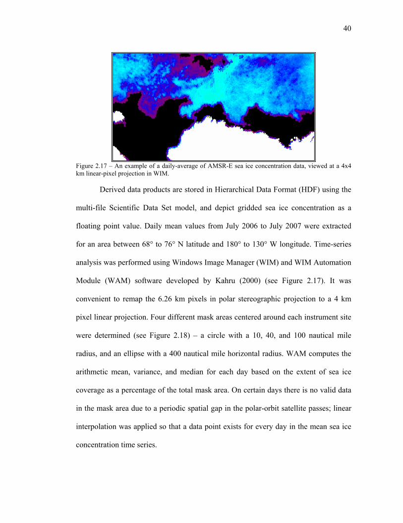
Figure 2.17 – An example of a daily-average of AMSR-E sea ice concentration data, viewed at a 4x4 km linear-pixel projection in WIM. Derived data products are stored in Hierarchical Data Format (HDF) using the

multi-file Scientific Data Set model, and depict gridded sea ice concentration as a

floating point value. Daily mean values from July 2006 to July 2007 were extracted

for an area between 68° to 76° N latitude and 180° to 130° W longitude. Time-series

analysis was performed using Windows Image Manager (WIM) and WIM Automation

Module (WAM) software developed by Kahru (2000) (see Figure 2.17). It was

convenient to remap the 6.26 km pixels in polar stereographic projection to a 4 km

pixel linear projection. Four different mask areas centered around each instrument site

were determined (see Figure 2.18) – a circle with a 10, 40, and 100 nautical mile

radius, and an ellipse with a 400 nautical mile horizontal radius. WAM computes the

arithmetic mean, variance, and median for each day based on the extent of sea ice

coverage as a percentage of the total mask area. On certain days there is no valid data

in the mask area due to a periodic spatial gap in the polar-orbit satellite passes; linear

interpolation was applied so that a data point exists for every day in the mean sea ice

concentration time series.

41

Figure 2.18 – Mask areas used to perform time series analysis on AMSR-E sea ice concentration data. Three circles were centered over the HARP sites, shown from left to right with radii of 10, 40, and 100 nautical miles. Discrete or continuous random time series have several statistical properties

that help characterize the variability of the series and allow for comparison between

one another. The correlation function describes the covariability of given time series

as functions of two different times, t and t + ", where " is the lag time. It uses the

“raw” data series before removal of the mean, as opposed to the covariance function.

If y(t) is a stochastic time series consisting of N values, the autocorrelation function

Ryy is expressed as

,

where for is the lag time for k sampling time increments, ,

and . In general, the autocorrelation function will be more strongly correlated

than the original time series y(t). Replacing one of the y(t) with another function x(t),

the cross-correlation function Rxy between two time series is expressed as

.

Daily or weekly samples are not necessarily independent, so in order to

determine the number of independent sea ice coverage and acoustic pressure level

samples at each site, the integral time scale must be computed from autocorrelations of

Ryy (( ) = 1N ! k

(yi yi+ k )i=1

N ! k

'

( = ( k = k*t !k = 0,K , M *t

!M = N

Rxy (( ) = 1N ! k

(yi xi+ k )i=1

N ! k

'

42

the sea ice concentration and acoustic pressure level data. The integral time scale T is

defined as the sum of the normalized autocorrelation function $yy over the length

of the time series for N lag steps, . The estimate is expressed as

,

where provides a measure of the dominant correlation time scale within

the time series – for times longer than T, the data become decorrelated. In general, the

summation should continue until it reaches a near-constant value, which is taken as the

value for T. The number of instrument deployment days is divided by the calculated

integral time scale to determine degrees of freedom (i.e. bin size) within the time

series, or the number of independent samples at each site (Emery and Thomson,

1998).

Sea ice concentration data had a longer integral time scale for independence of

estimates at both sites than did acoustic pressure levels, ranging from two to three days

depending on the size of the mask area. Pearson’s coefficient of correlation was

binned into two-day periods corresponding to the integral time scale. A t-test

evaluated the null hypothesis that sea ice concentration and acoustic pressure levels

are not related, using significance level # = 0.05.

Barrow Wind Speed Data

Wind data was obtained from the U.S. National Weather Service at the NOAA

Alaska Region Headquarters. Meteorological variables were measured at location 71°

L = N*( *(

T = *(2

+yy(( i ) + +yy (( i+1)!" $%i=0

N '

'

N ' ' N ! 1

43

17’07” N, 156° 45’57” W, by an Automated Surface Observing System (10 meters

above sea level) at Wiley Post-Will Rogers Memorial Airport in Barrow, AK, which is

approximately 60 nautical miles south of the instrument sites. This separation between

recording sites may result in minor error. Daily-value time series ranging from July

2006 to July 2007 were collected for weather elements including peak wind speed

(knots), average wind speed (knots), and peak wind direction.

Statistical time series analysis could not be performed on daily-averaged wind

speed since only one data point exists for each day, but there was still interest

nonetheless to determine if cross-correlations exist between wind speed and acoustic

pressure levels at different frequency bands. The comparison was binned into two-day

intervals so that the role of sea ice influencing the correlation between wind and

ambient noise could also be examined with the same number of independent samples.

Sound Speed Profiles

The most significant environmental factor influencing acoustic measurements

in the open ocean include refraction effects caused by thermal gradients. Albers (1965)

emphasized that bathythermograph measurements should be included with all acoustic

measurements made in the ocean so that corrections for refraction can be applied to

the measurements.

While underway on the Healy in September 2007, vertical sound speed profile

measurements were conducted at both instrument sites and several other locations in

the Chukchi Sea (see Figure 2.19). These profiles cannot be representative of sound

44

speed at other times throughout the year since water temperatures can fluctuate

substantially in response to changes in sea ice coverage and solar radiation (i.e. ice

albedo). The thermocline is probably shallower and subtle in winter, while deeper and

more pronounced in summer. As with any scientific measurement in the Arctic Ocean

though, it’s always more difficult to collect vertical profile data during the winter

season.

Figure 2.19 – Vertical depth profiles for water temperature (left) and sound speed (right) were measured by XBT probes during the summer of 2007. Measurements were collected using expendable AN/SSQ-36B

bathythermograph sonobuoys, a low-cost method for obtaining vertical temperature

profiles. The 16-pound (7.3 kg) units are easily deployed from the deck of a surface

vessel and provide a thermal gradient measurement scheme. Thirty seconds after water

entry at the surface, a probe activates and descends at a rate of 1.5 m/sec (5 ft/sec).

The buoy has an operating life of approximately 12 minutes, which allows the probe to

reach depths between 0 and 800 meters (2625 ft). Thermistors located in the probe

measure changes in seawater temperature during descent with a calibrated sensor

45

accuracy of ±0.55° C (±1° F). VHF transmissions at 0.25 W are received via RF

transmittal to a radio station aboard the surface vessel. The data can be processed and

displayed as temperature versus depth using the following relationships:

temperature (°F), and depth (m), ,

where f is sound frequency transmitted and t is the length of time during transmission.

The speed of sound in seawater depends on pressure (i.e. depth) and temperature ($1°

C ~ 4 m/s) to first order, and salinity ($1‰ ~ 1 m/s) to second order. An empirical

equation derived by Mackenzie (1981) accurately calculates sound speed from these

variables (higher order terms using salinity measurements are neglected), given as

2 2 4 3

2 7 2 13 3

( , ) 1448.96 (4.591) (5.304 10 ) (2.374 10 )(1.63 10 ) (1.675 10 ) (7.139 10 )

c T z T T Tz z Tz

! !

! ! !

= + ! , + ,+ , + , ! ,

.

T = f ! 80020 z = (1.5m / s) * t

46

III. RESULTS

Ambient Noise Measurements

Due to an inductor – onboard the hydrophone’s pre-amplifier circuit – failing

during deployment from freezing temperatures, ocean ambient noise was not recorded

in the frequency band between 250-3000 Hz. Instead only self-noise was recorded in

the circuit tank, so therefore data will not be reported at these frequencies. Spectral

plots are instead presented for a low-frequency band (10-250 Hz) and high-frequency

band (3-16 kHz). It was also unanticiaped that alkaline batteries would be pushed

beyond their operating conditions, but since there was consistent water temperatures

of -2° C, the voltages eventually drained below the sufficient amount needed to draw

current to the hard drives. Therefore, the site A instrument was only able to record

data for five months while the site B instrument recorded for nine months.

Background-noise levels are shown in Figures 3.1 and 3.2 for site A from

September, 2006 – January, 2007 and site B from September, 2006 – May, 2007. All

acoustic events, transient signals, and electronic noise were removed from the spectral

averages, in addition to applying a transfer function to correct for received pressure

levels. In summer and early fall, broadband sources like storm-generated winds and

surface waves couple with the underwater noise environment, but from late fall to late

spring, it is the state of sea ice that inevitably influences the complex relationship

between ambient noise and the environment. At 10 Hz, the site A spectra converge

around 85-88 dB re µPa while site B is spread out between 80 and 93 dB re µPa.

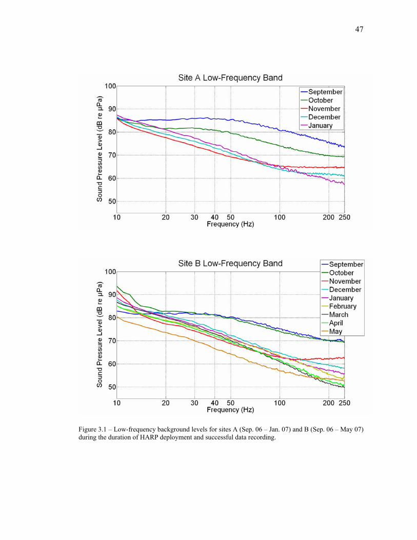
47

Figure 3.1 – Low-frequency background levels for sites A (Sep. 06 – Jan. 07) and B (Sep. 06 – May 07) during the duration of HARP deployment and successful data recording.

48

Across the entire low-frequency band, September and October are naturally the

noisiest months – due to open-sea conditions – reaching peak noise-levels of 87 dB re

µPa between 20 and 60 Hz at site A (see Figure 3.1). All other months that were

recorded exhibit low spectrum levels, as sound-pressure levels decrease linearly

approximately 8 dB/octave as frequency increases logarithmically. Typical levels for

both sites at 50 Hz are shown to be slightly above or below 70 dB re µPa, with May

reaching as low as 65 dB re µPa. By 200 Hz, noise levels at site B are as low as almost

50 dB re µPa in March, the month where sea ice extent reaches its maximum. The

steep spectral slopes of ambient noise are most likely attributed to sea ice coverage in

the region around the two instruments.

Heavy pack and shore-fast ice act like a rigid boundary for sounds propagating

horizontally across the waveguide, except that the underside of sea ice is rough and

dispersed with ridges and keels. As frequency increases so does scattering strength and

thus transmission loss; plane waves that reflect off ice tend to attenuate rapidly and

transmit over shorter distances. Figure 3.2 demonstrates that there is little variability

between different months in the high-frequency band. Besides September, nearly

every month at Site B converges and noise-spectrum levels are characterized as 63 dB

re µPa at 3 kHz, 52 dB re µPa at 10 kHz, and drops off even further to as low as 45 dB

re µPa at 15 kHz. At site A, there is a consistent spacing interval between sound-

pressure level curves across the frequency band, which decrease in order from

September through January.

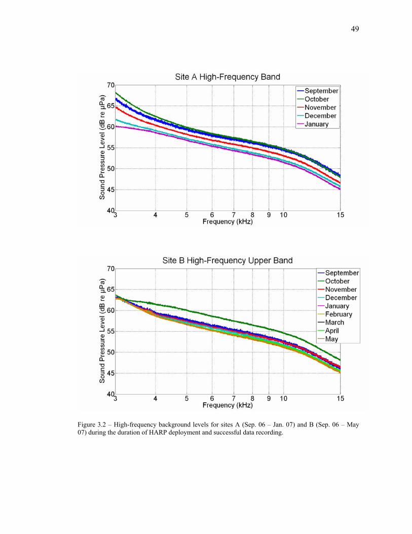
49

Figure 3.2 – High-frequency background levels for sites A (Sep. 06 – Jan. 07) and B (Sep. 06 – May 07) during the duration of HARP deployment and successful data recording.

50

Figure 3.3 – Site B Low-Frequency Noise Distributions. Seismic airguns are present from Sep. to Nov., while 10% of Oct. is exposed to noise above 130dB re µPa at 10Hz and 112dB re µPa between 20–30Hz. The harmonics present in Nov., Feb., and May are indicative of hydrophone strum noise. Background levels decrease approximately 8dB/octave, reaching 70dB re µPa at 10Hz and under 50dB re µPa between 150–250Hz.

51

Figure 3.3 – Continued

52

Figure 3.4 – Site A Low-Frequency Noise Distributions. Much less transient energy was received compared to site B, possibly due to differences in bathymetry. Sep. and Jan. are good examples of a near-Gaussian distribution across the frequency band since the spectral curves are spaced apart evenly from the mean measurement. Most months for both sites exhibit non-Gaussian behavior due to a low background environment interposed by impulsive transient events such as dynamic sea ice mechanisms and man-made noise.

53

Figures 3.3, 3.4, 3.5, and 3.6 represent statistical pressure-density distributions

for every month, each containing approximately 17,000 spectral-averaged, 200 sec

samples. Sound-pressure spectrum levels are shown for distribution percentiles for the

highest 1% (99%), upper 10% (90%), median (50%), lower 10%, lowest 1%, and

mean distribution. Deviation of the mean from the median illustrates the assymetry of

the density peak from Gaussian normal, while the upper and lower percentiles describe

the shape of the tails. Because of the unique properties inherent in Arctic transmission

loss, oceanic ambient background-noise is typically very low and characterized by a

steeply decreasing slope as frequency increases. The composite of impulsive transient-

sound events noticeably stands out above the ambient noise spectrum. Certain months

have spectral-energy peaks at varying frequencies, which can be attributed to different

acoustic sources such as the dynamic processes of sea ice, intermittent anthropogenic

noise, and possibly marine mammal vocalizations at stereotypic calling bands. These

transient signals will be discussed in the analysis section.

54

Figure 3.5 – Site B High-Frequency Noise Distributions. Comparing noise levels to the similar background levels in Figure 3.2 show that transient signals do not really influence high-frequency ambient noise since attenuation is so high. At 3 kHz, noise levels range between 60–65dB re µPa, converge to around 50dB re µPa at 10 kHz, and decrease to less than 45dB re µPa at 15 kHz. Note that the frequency spikes are attributed to electronic instrument noise and should not be considered.

55

Figure 3.5 – Continued

56

Figure 3.6 – Site A High-Frequency Noise Distributions. For every month, the 99th percentile is measured well above mean and median spectrum levels, and is indicative of highly-impulsive and localized noise sources being received through direct ray path transmission by the hydrophone. In September, impulsive noise is derived from wind-driven wave interactions with the MIZ, while in January thermal fracturing is responsible for this non-Gaussian distribution.

57

Environmental Correlates

The three plots in Figure 3.7 show time series for acoustic pressure-levels

simaltaneously with average wind speed and sea ice concentration data. The spatial

areas used for time series analysis of sea ice coverage were chosen based upon the

potential propagation range appropriate for three different frequency bands – 25 Hz

over 100 nautical miles, 100 Hz over 40 nautical miles, and 5 kHz over 10 nautical

miles.

During summer and fall when sea ice has retreated north and open-ocean

conditions prevail (September through November), the peaks and troughs of sound-

pressure spectrum levels correlate directly with those of high wind speed values,

especially in early October; typically strong winds are indicative of storms or other

low-pressure weather patterns. Throughout winter and spring, large-scale thermal

fracturing opens up leads and causes sea ice coverage to sporadically decline for short

periods, as a result of atmospheric circulation and wind-stress forcing. For cases such

as in early February, the spectral energy-peaks of sound correlate very well with high

wind speeds, but still depend foremost on sea ice conditions. During sea ice pack

formation and subsequent pressure ridging in the fall, high-frequency noise levels

around 5 kHz respond substantially to these localized noise-generating mechanisms. In

fact, spectral-energy peaks in this frequency band seem to correlate best with wind

speed, and occur across greater temporal variability. When sea ice maintains 100%

coverage in the surrounding area and wind speed values are low, no correlations exist

and ambient noise has reached its lowest sound-pressure levels.

58

Figure 3.7 – Time series of sound-pressure spectrum levels (top/dark blue) for three different frequencies (25, 100, 5000 Hz) plotted with daily-average wind speed values (middle/green) over Barrow, as well as the percentage of sea ice coverage (bottom/light blue) for a specified area (10, 40, 100 nautical mile radius) centered around the instrument sites. Note that for the 5 kHz band, flat noise levels at 57 dB re µPa in the spectral time series indicate the noise floor of the HARP was reached, so in actuality it can be assumed that ambient noise levels at this frequency extend several dB below what is reported here.

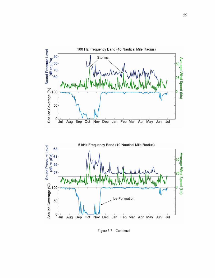
59

Figure 3.7 – Continued

60

IV. ANALYSIS

Figure 4.1 – Time scales of noise-generating mechanisms

Man-Made Seismic & Low-Frequency Noise

Airguns are used for seismic marine reflection and refraction surveys, which

are currently taking place each summer across vast Arctic coastal regions for oil and

natural gas exploration. The device consists of pneumatic chambers pressurized with

air. An array of multiple airguns is submerged below the sea surface and towed behind

a ship; when the air gun is fired, a bolt is retracted, allowing compressed air to escape

the chamber and release a burst pulse of instantaneous high-acoustic energy.

According to modal theory, if the seismic source is near the sea surface, then

only sound waves with quarter wavelengths longer than the water depth will penetrate

the earth. This is of course frequency dependent, so if a vessel is conducting a seismic

survey on the continental shelf of Alaska’s North Slope – where the average depth is

between 50 and 100 m – then theoretically around 7 or 8 Hz acoustic waves will

reflect off the seafloor and propagate over great distances through the waveguide.

Since it is completely open water (i.e. nearly perfect reflector) during summer in a

shallow waveguide, the effects of Arctic transmission loss no longer apply, and the

residual energy of airgun shots become trapped in the water column during

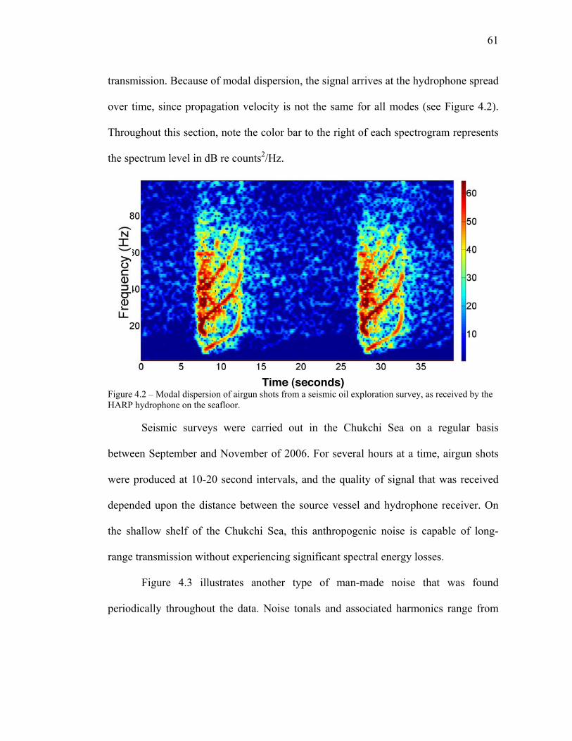
61

transmission. Because of modal dispersion, the signal arrives at the hydrophone spread

over time, since propagation velocity is not the same for all modes (see Figure 4.2).

Throughout this section, note the color bar to the right of each spectrogram represents

the spectrum level in dB re counts2/Hz.

Time (seconds)

Figure 4.2 – Modal dispersion of airgun shots from a seismic oil exploration survey, as received by the HARP hydrophone on the seafloor. Seismic surveys were carried out in the Chukchi Sea on a regular basis

between September and November of 2006. For several hours at a time, airgun shots

were produced at 10-20 second intervals, and the quality of signal that was received

depended upon the distance between the source vessel and hydrophone receiver. On

the shallow shelf of the Chukchi Sea, this anthropogenic noise is capable of long-

range transmission without experiencing significant spectral energy losses.

Figure 4.3 illustrates another type of man-made noise that was found

periodically throughout the data. Noise tonals and associated harmonics range from

62

10-150 Hz, produced from rotating or reciprocating machinery generated by ships

radiating sound underwater, or by snowmobile engines coupling through the ice.

Time (seconds)

Figure 4.3 – Tonals like these have the acoustic signature of recipricating machinery.

Microseisms & Earthquakes

Low seafloor noise levels above 5 Hz provide a band for detection of small-

magnitude local and regional earthquakes, which may have energy at frequencies

extending up to 50 Hz (Webb, 1992). Webb proposed that most energy in the

microseism band propagates from a wide source region in the Gulf of Alaska. Large

earthquakes generate wave trains that occasionally dominate the sound-pressure

spectrum across low frequencies, peaking at about a 25 second period (Webb, 1992).

Short-period microseism noise – usually related to storms at sea – falls

significantly during periods of very light winds. Arctic seafloor measurements in the

teleseismic frequency band (10-3 – 101 Hz) during winter show that the generation of

microseisms is suppressed due to near-continuous ice coverage preventing the

63

excitation of ocean waves; Arctic seafloor sound-pressure levels in the microseism

band provide possibly some of the quitest seismic sites on Earth (Webb, 1992). As a

result, teleseismic noise levels on the Arctic basin are 20 dB less than those typical of

the Atlantic Ocean and 40 dB less than those typical of the Pacific (Webb and Schultz,

1992). Figure 38 shows that the spectra of pressure fluctuations measured from the

seafloor of the Beaufort Sea are unenergetic in comparison to measurements from the

Pacific or Atlantic (Webb, 1992). At 10 Hz, noise levels in the Arctic are

approximately 87 dB re 1 µPa2/Hz, which match well with the measurements shown in

Figure 4.4.

Figure 4.4 – Pressure spectra from the Pacific, Atlantic, and Arctic seafloors. The microseism peak is evident between 0.1 and 5 Hz. At 10 Hz, noise levels in the Arctic are approximately 87 dB re 1 µPa2/Hz (Webb, 1992).

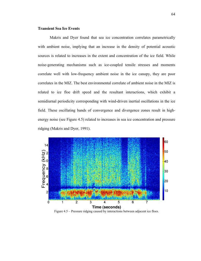
64

Transient Sea Ice Events

Makris and Dyer found that sea ice concentration correlates parametrically

with ambient noise, implying that an increase in the density of potential acoustic

sources is related to increases in the extent and concentration of the ice field. While

noise-generating mechanisms such as ice-coupled tensile stresses and moments

correlate well with low-frequency ambient noise in the ice canopy, they are poor

correlates in the MIZ. The best environmental correlate of ambient noise in the MIZ is

related to ice floe drift speed and the resultant interactions, which exhibit a

semidiurnal periodicity corresponding with wind-driven inertial oscillations in the ice

field. These oscillating bands of convergence and divergence zones result in high-

energy noise (see Figure 4.5) related to increases in sea ice concentration and pressure

ridging (Makris and Dyer, 1991).

Time (seconds)

Figure 4.5 – Pressure ridging caused by interactions between adjacent ice floes.

65

The production of high-frequency noise increases almost immediately

following decreases in air temperature and cloud cover conditions – typically

associated with lower wind speeds – thus altering the radiation heat balance. However,

thermal fracturing can be greatest when sensible heat flux – during periods of

atmospheric warming – helps to warm sea ice prior to the onset of heat loss and rapid

cooling (Lewis and Denner, 1988). The profusion of small-scale cracks originates

from the hummocks and angular projections of pack ice, while longer cracks come

from the uniform surfaces of frozen leads (Milne and Ganton, 1964). High spatial

variability of such noise is likely the result of uneven snow cover due to wind forcing.

In winter, Gaussian “white” noise can be generated by the wind-induced

motion of drifting granular snow being blown over rough sea ice, but this process is

often masked during periods of decreasing air temperatures by high-energy impulsive

events that reach spectral energy-peaks up to 40 dB above the Gaussian background. If

air temperatures rise though, impulsive thermal ice fracturing noise tends to disappear

(Milne and Ganton, 1964). The effects of thermal stress are found to be less prevalent

in spring and summer than in winter, where thermally induced noise is prominent in

the 2-15 kHz frequency band (see Figure 4.6); another correlate above 1 kHz is

attributed to wind (Milne and Ganton, 1964).

66

Time (seconds)

Figure 4.6 – Thermal fracturing due to atmospheric cooling.

Wind-Driven Noise

During fall, the ice pack receives a fresh blanketing of snow from advancing

weather fronts. It is actually Arctic winds that then tend to strip snow from flatter

regions while deposits of snow build up around the ridges and hummocks of pack ice;

thus snow thickness exhibits a large variance in its spatial distribution. Lewis and

Denner proved through their model of Arctic sound transmission that snow cover can

consistently alter the degree in which sea ice responds to atmospherically induced

thermal fracturing. Their heat-flux balance at the surface included short-wave solar

radiation, long-wave atmospheric radiation, and long-wave ice radiation (i.e. albedo).

Without snow cover, temperatures at the ice surface would drop due to reductions in

cloud coverage or air temperature. Sensible heat flux from the atmosphere caused pack

ice to warm whenever strong wind fronts approached. (Lewis and Denner, 1988)

67

The moments due to opposing wind and current stresses acting on sea ice

correlate well with low-frequency noise generated from pack ice (Makris and Dyer,

1986). Ganton and Milne estimated – based on surface roughness and free-stream

wind velocity – that for a Reynolds number greater than 125, the onset of wind at

speeds ranging from 3-5 mph will penetrate the laminar sublayer of snow cover and

prompt vortices to shed, thus producing noise coupled through the ice beneath (see

Figure 4.7). Average wind speeds in the Arctic resemble a “white” Gaussian-noise

distribution, and are attributed to be the major source of noise centered at 10 kHz

(Ganton and Milne, 1965). Although wind-driven noise is much more pronounced

under noncontinuous ice cover, according to Macpherson, ambient noise levels

become independent of wind speed during periods of continuous pack ice coverage

(Kibblewhite and Jones, 1976).

Time (seconds)

Figure 4.7 – Storm-generated winds produce noise related to snow blowing over ice or leads opening.

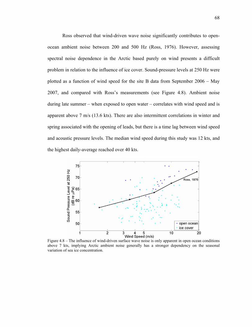
68

Ross observed that wind-driven wave noise significantly contributes to open-

ocean ambient noise between 200 and 500 Hz (Ross, 1976). However, assessing

spectral noise dependence in the Arctic based purely on wind presents a difficult

problem in relation to the influence of ice cover. Sound-pressure levels at 250 Hz were

plotted as a function of wind speed for the site B data from September 2006 – May

2007, and compared with Ross’s measurements (see Figure 4.8). Ambient noise

during late summer – when exposed to open water – correlates with wind speed and is

apparent above 7 m/s (13.6 kts). There are also intermittent correlations in winter and

spring associated with the opening of leads, but there is a time lag between wind speed

and acoustic pressure levels. The median wind speed during this study was 12 kts, and

the highest daily-average reached over 40 kts.

Figure 4.8 – The influence of wind-driven surface wave noise is only apparent in open ocean conditions above 7 kts, implying Arctic ambient noise generally has a stronger dependency on the seasonal variation of sea ice concentration.

69

Bioacoustic Detections

All species of marine mammals found in the Western Arctic produce

characteristic calls that can be used for acoustic identification (Stirling 1983,

Bel’kovitch 1993, Moore et al. 2006, Clark et al. 1996). Long-term averaged spectral

time series were scanned visually for the presence of known call-types for the five

most common species in the area of study – the bowhead whale, beluga whale,

bearded seal, ringed seal, and walrus. Each detection was logged and the species

identification confirmed by audio playback through headphones. Acoustic detections

were grouped into hourly bins for the three most readily identified species –

bowheads, belugas, and bearded seals – and the number of hours per day during which

calls were detected, were plotted for each of these species.

Although extensive recordings have been made north of Barrow between April

and June over the past 18 years (Van Parijs, Clark 2006), little or no acoustic

recording has been undertaken in this area between the months of November and

April. With the addition of winter and spring months, detection time series for

bowheads, belugas, and bearded seals are presented along with representative

spectrograms of recorded calls for late Sepember 2006 through the end of May 2007.

Comparing the time series of detected calls for each species to environmental

correlates (see Figure 3.7), especially the extent of sea ice coverage, provides some

interesting insights into the timing of species movements and seasonal acoustic

behavior.

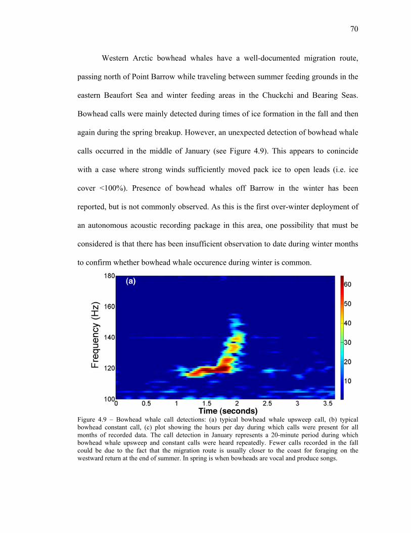
70

Western Arctic bowhead whales have a well-documented migration route,

passing north of Point Barrow while traveling between summer feeding grounds in the

eastern Beaufort Sea and winter feeding areas in the Chuckchi and Bearing Seas.

Bowhead calls were mainly detected during times of ice formation in the fall and then

again during the spring breakup. However, an unexpected detection of bowhead whale

calls occurred in the middle of January (see Figure 4.9). This appears to conincide

with a case where strong winds sufficiently moved pack ice to open leads (i.e. ice

cover <100%). Presence of bowhead whales off Barrow in the winter has been

reported, but is not commonly observed. As this is the first over-winter deployment of

an autonomous acoustic recording package in this area, one possibility that must be

considered is that there has been insufficient observation to date during winter months

to confirm whether bowhead whale occurence during winter is common.

(a)

Time (seconds) Figure 4.9 – Bowhead whale call detections: (a) typical bowhead whale upsweep call, (b) typical bowhead constant call, (c) plot showing the hours per day during which calls were present for all months of recorded data. The call detection in January represents a 20-minute period during which bowhead whale upsweep and constant calls were heard repeatedly. Fewer calls recorded in the fall could be due to the fact that the migration route is usually closer to the coast for foraging on the westward return at the end of summer. In spring is when bowheads are vocal and produce songs.

71

(b)

Time (seconds)

(c)

Figure 4.9 – Continued

Belugas from the eastern Chuckchi Sea have been observed by aerial surveys

and satellite tracking to prefer the edge of the pack ice, but also to travel in open water

as well as hundreds of kilometers into 90% ice cover (Suydam et al. 2001). As

expected, beluga calls were detected throughout times of open water and into the late

fall and early spring during ice formation and breakup. Beluga clicks and whistles

were commonly present up until mid-November, occured again in early December

after the ice cover had reached 100% and receded slightly, and then were not detected

again until mid-April (see Figure 4.10).

72

(a)

Time (seconds)

(b)

Time (seconds) Figure 4.10 – Beluga whale call detections: (a) whistles, (b) clicks and whistles, (c) plot showing the number of hours per day during which beluga calls were present for all months of recorded data.

73

(c)

Figure 4.10 – Continued

Male bearded seals exhibit seasonal acoustic behavior associated with mating.

This has been reported to take place most commonly from April to July (Van Parijs et

al. 2001) with calls reported as early as late winter (Stirling, 1983). During this time

males produce four categories of vocalizations – trills, ascents, sweeps, and moans.

These calls are highly stereotyped with stocks having distinct repertoires that have

remained stable on decadal timescales (Risch et al. 2007).

Most previously described bearded seal call-types for the western Arctic

(Risch et al. 2007) were present in the data during the spring as expected, but also

from December through the end of February. This mid-winter calling behavior has not

been reported to date, which could be due to the fact that long-term recordings have

not been made in this area earlier than April. One additional highly-stereotyped call

was recorded during a two-week period of ice formation in November (see Figure

4.11a). This is likely a bearded seal sweep that has not been described for this

population to date.

74

(a)

Time (seconds)

(b)

Time (seconds) (c)

Figure 4.11 – Bearded seal call detections: (a) typical early winter bearded seal downsweep (Nov-Dec), (b) bearded seal trills, (c) plot showing the hours per day during which bearded seal calls were present for all months of recorded data.

75

Time (seconds)

Figure 4.12 – Representative spectrogram of a commonly encountered ringed seal calling sequence in which multiple low-frequent barks are interspersed with higher frequency yelps.

Time (seconds)

Figure 4.13 – Spectrogram showing a rapid series of walrus knocks. Although walrus are known to produce a variety of sounds, including the unique bell-like call of the male, this rapid knocking represents the predominant walrus call in the dataset.

76

V. DISCUSSION

Arctic Sound Propagation

Because of the combination of upward refraction, under-ice reflection, and

high scattering strength, long-range sound propagation is highly dependent on the state

of sea ice. Therefore transmission loss may increase at a rate faster than cylindrical

spreading as frequency increases (see Figure 5.1); thus high-frequency acoustic waves

will attenuate with increased range (Yang and Votaw, 1981). Reflection and

transmission coefficients are typically dependent on interactions with the boundary

interfaces, but in the Arctic they are generally proportional to the thickness of sea ice,

and as a result determine the shape of the frequency-dependent ambient noise

spectrum (Diachok and Winokur, 1974).

Figure 5.1 – Transmission loss measurements versus range in the Arctic Ocean for various frequencies (Buck, 1968). Geometric spreading and bulk attenuation alone cause low-frequency

transmission loss in the Arctic waveguide by as much as 10-2 dB/km at 20 Hz and l0-1

dB/km at 80 Hz. Frequency dependence of such loss is proportional to f 1.5 or f 2

77

(LePage and Schmidt, 1994). The highly refractive upper duct – which extends about a

hundred meters into the water column layer – completely strips energy from trapped

ray bundles after propagating less than a hundred kilometers, leaving a residual field

of deeper diving rays. At shallow depths these rays are less excited and sound sources

couple most energy into the lower-order modes, thus surface interaction losses still

dominate at low frequencies (LePage and Schmidt, 1994). This mode stripping is the

result of lower-order modes being trapped in the surface channel and interacting

continuously with the underside of the ice cover, resulting in high scattering loss.

Higher-order modes are influenced by the deep pressure gradient associated with

convergence zone paths, and therefore interact less with the ice cover. This implies

that lower-order modes can be neglected when considering long-range propagation

(LePage and Schmidt, 1994). In a shallow-water waveguide there is a remarkable loss

of higher propagating modes in the 12.5-25 Hz band (Milne and Ganton, 1964).

Figure 5.2 – Ray paths from sources at the surface propagate directly to a bottom-mounted hydrophone. Angles are with respect to the surface. The bottom limiting ray grazed the ice-water surface at 9.5° with a range of 4.3 miles, enclosing a circular area of 59 square miles (Milne & Ganton, 1964). The contribution of high-frequency acoustic waves is largely the result of

noise-generating mechanisms from sea ice that propagate to the hydrophone by direct

ray paths. Lower frequencies around 10 Hz contribute from much farther distances,

78

with wavelengths in excess of the scale size for under-ice projection (Milne and

Ganton, 1964). According to Snell's law, acoustic rays can only propagate across

distances greater than 30 km in the ice-water interface if the grazing angle % is less

than 15° (see Figure 5.2). Reflection loss has to be much greater than zero because the

sea ice canopy is interspersed with rough ridges (Diachok, 1976). Statistically, the loss

per under-ice reflection is almost 15 dB when grazing angles are between ±7.5° and

±8.5°. Waves reflected off the seafloor make many more under-ice reflections (see

Figure 5.3) than those confined to refracted paths within the upper water column

(Milne and Ganton, 1964).

Figure 5.3 – An acoustic plane wave reflected from a random distribution of elliptical half-cylinders (Diachok, 1976).

Ambient Noise Level Distributions

It has been demonstrated that Arctic ambient noise varies uniquely from all

other ocean environments in regards to its spatial and temporal variability related to

sea ice and in many cases wind. Already during summer and early fall though, there is

significant acoustic energy derived from other transient signals, namely anthropogenic

noise sources. When examining the low-frequency spectral levels in Figures 3.3 and

3.4 compared to the background noise levels in Figure 3.1, it appears that September

79

should be the noisiest month based on the natural variability of sea ice and wind in

space and time, but in actuality the October sound-spectrum experiences substantially

higher noise-levels primarily due to the residual energy of seismic exploration

reflecting off the seafloor and propagating through the waveguide.

Buck and Wilson reported ice cracking noise levels near a ridge to be 100 dB

at 10 Hz; Lewis and Denner also detected noise levels at 10 Hz as high as 100 dB in

winter; Makris and Dyer observed a broad peak associated with ice cracking around

15 Hz reaching 90 dB. Background noise levels in Figure 3.1 vary above and below 87

dB re µPa at 10 Hz and are consistent with the tail end of Webb’s microseism band,

but by observing the density distributions for all transient acoustic events present in

the data, ambient noise levels can reach upwards of 150 dB re µPa to as low as 70 dB

re µPa. The shape of spectral background-noise in the 10-50 Hz band is normally

attributed to the influence of distant global shipping for Pacific deep-ocean ambient

noise (McDonald, 2006). Since the shallow waters of the Bering Sea prevent this

trans-oceanic propagation from being introduced to the Arctic underwater

environment, there is no explicit frequency band attributed to the influence of ship

cavitation noise.

Noise levels for nearly every month are shown to be non-Gaussian below 20

Hz since the mean sound-pressure levels are above that of the median and translate

into a shift of the distribution peak to the right. In addition, the contributions of

localized high-energy impulsive noise to the sound spectrum imply that the

distribution function is long-tailed on the right side. Building upon the concept of

80

Dyer’s statistical sound transmission, since multipath propagation is affected so much

by high under-ice scattering strengths, then the lower spectral levels for nearly every

month generally exhibit the same shape and are often close to median levels, implying

the distribution function is short-tailed on the left side. For certain months, probability

densities were very broad and were found to resemble chi-square distributions. As

frequency increases and extends into higher bands, the ambient noise level density

distributions become closer to near-Gaussian levels.

Sea Ice Kinematics

The dynamics of sea ice determine its extent, concentration, thickness, rigidity,

and variations throughout different seasons and regions, thus introducing causality on

both temporal and spatial scales. One noise-generating mechanism can produce

broadband spectral energy across many frequencies, which in turn can mask other

noise variations induced by a different mechanism. For instance, fluctuations in

thermal fracturing of sea ice for a given air temperature is highly regionally

dependent, but during non-summer months when acoustic-noise amplitudes reach

pressures greater than 103 Pa, thermal fracturing is the dominant noise source

responsible for Arctic ambient noise episodes at 1 kHz (Lewis and Denner, 1988).

Pack ice consists of seasonal and perennial (i.e. multiyear) floes up to 2-3

meters thick in near-continuous contact over large areas of the high Arctic, and

interspersed with pressure ridges heaped together by piled rubble formed through

collisions and shear interactions between adjacent floes (see Figure 5.4). These ridges

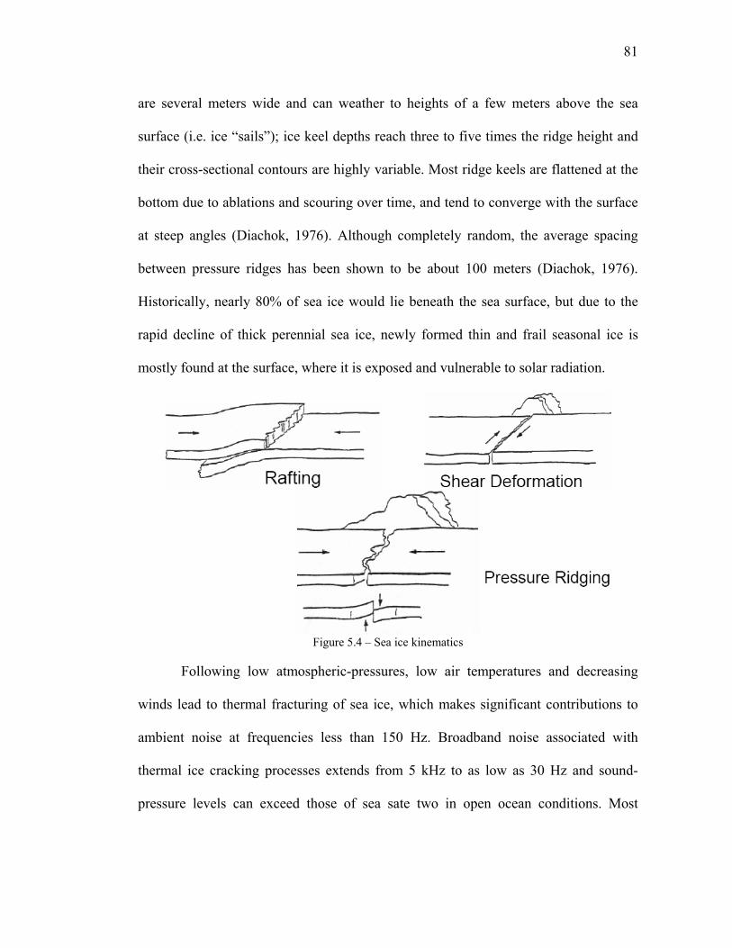
81

are several meters wide and can weather to heights of a few meters above the sea

surface (i.e. ice “sails”); ice keel depths reach three to five times the ridge height and

their cross-sectional contours are highly variable. Most ridge keels are flattened at the

bottom due to ablations and scouring over time, and tend to converge with the surface

at steep angles (Diachok, 1976). Although completely random, the average spacing

between pressure ridges has been shown to be about 100 meters (Diachok, 1976).

Historically, nearly 80% of sea ice would lie beneath the sea surface, but due to the

rapid decline of thick perennial sea ice, newly formed thin and frail seasonal ice is

mostly found at the surface, where it is exposed and vulnerable to solar radiation.

Figure 5.4 – Sea ice kinematics

Following low atmospheric-pressures, low air temperatures and decreasing

winds lead to thermal fracturing of sea ice, which makes significant contributions to

ambient noise at frequencies less than 150 Hz. Broadband noise associated with

thermal ice cracking processes extends from 5 kHz to as low as 30 Hz and sound-

pressure levels can exceed those of sea sate two in open ocean conditions. Most

82

thermal stress occurs within the upper 20 cm of sea ice. It has been shown that 30% -

40% of acoustic noise events in non-summer months correspond with changes in heat

flux (Lewis and Denner, 1988). Transmission in the 32-Hz frequency band reaches

length scales of 660 km in fall and 1000 km in spring (Lewis and Denner, 1988),

while high-frequency fracture noise can propagate over ranges of approximately 150

km during the fall season, increasing to 300 km in spring. Thermal fracturing appears

to dominate noise transmission during non-summer months, as opposed to motion-

induced fracturing, but the natural variability in atmospheric forcing decides these

length scales.

It is not entirely the temperature value itself, but in fact the rate or flux of

decrease in air temperature over time that produces fracturing due to thermal stress;

this corresponds with large increases in impulsive noise (Ganton and Milne, 1965).

Milne and Ganton observed that the production of tensile cracks associated with this

impulsive noise is characterized by a Poisson density distribution over time. Under

rising air temperatures, the sporadic nature of this noise disappears and a near-

Gaussian distribution reappears (Kibblewhite and Jones, 1976). In the fall and winter

seasons, thermal fracturing processes involve the loss of heat as a result of long-wave

radiation, whereas the spring season is subjected to a combination of atmospheric

short-wave solar radiation, snow cover, and long-wave radiation, driving thermal

waves into the sea ice. The resulting fracture noise can be radically modified on a

daily basis as a result of meteorological conditions such as cloud cover and blowing

snow (Lewis and Denner, 1988).

83

The slow fracturing of hardened pack ice over several tens of kilometers –

resulting in open leads – releases tremendous amounts of acoustic spectral-energy.

Thermal ice-cracking noise however, is more localized and propagates on the order of

meters or tens of meters, generating less spectral-energy per crack than lead-forming

fractures. In order for ice to crack, its temperature must be lower than typically -23 °C,

but also depends on the thickness of the pack ice (Zakarauskas et al. 1991).

Makris and Dyer described the behavior of sea ice concentration on short

spatial and temporal scales through semidiurnal inertial oscillations of ice floes in free

drift. Meunch et al. speculated that long internal waves originating near the ice edge at

the sea surface may be generated by wind-stress forcing, thereby advecting the ice

field into bands of alternating convergence and divergence zones. It was shown that

the generation mechanism for long internal waves was absent in the presence of wind-

driven surface gravity waves (Makris and Dyer, 1991).

Shifts in Sea Ice & Waveguide Propagation

The viability of sea ice in the Arctic Ocean – namely the thickness and

concentration of perennial ice coverage – is crucial in allowing the water column to

retain thermal energy by limiting melt and evaporation at the surface layer. The ice

albedo effect is a vital process necessary to prolonging the stability of thermohaline

circulation between the exchange of cold salty bottom water in polar regions and

warm fresh surface water in equatorial regions. Simply put, sea ice plays a pivotal role

in the Earth’s water cycle. This study recognizes that critical importance, but

84

endeavors to take a different approach than large-scale remote sensing by exploring

the intricate seasonal variability inherent in correlations between local sea ice

conditions and ambient sound-pressure levels that acousticians like Milne and Ganton

first observed in the 1960s.

As the rate in which the disappearance of multiyear pack ice increases due to

warming climate regimes, sea ice thickness will be considerably reduced and the ice

field will become more susceptible to solar heat radiation. If the strength of ice albedo

is diminished, then melt ponds will form due to surface interactions with air

temperature. These bodies of water will in turn absorb sensible heat flux exchange and

sea surface temperatures will rise. Thermal breakup, melt, and evaporation will begin

to occur earlier in spring each year because of this positive feedback mechanism, and

will also cause ice formation to occur later in fall depending on the variability of

atmospheric circulation. Once the majority of historic multiyear ice is replaced by frail

seasonal ice floes, water temperatures may consistently increase over many months

throughout the year, and feedback may occur exponentially in time.

The unique seasonal and temporal variability associated with noise spectrum

levels in the Arctic underwater sound environment will begin to also disappear during

many months of the year, and eventually may resemble ambient noise in the open

ocean more so than when subjected to ice cover. The rough surface boundary layer of

sea ice – which generally scatters and attenuates sound waves subjected to under-ice

reflections – will be replaced by the common air-water interface – a nearly perfect

reflector due to such a significant density gradient. Transmission loss will decrease

85

substantially and long-range propagation will contribute more to ambient noise levels.

Additionally, the continental shelf north of Alaska is only 50-100 m deep, so shallow-

water propagation will trap acoustic energy in the waveguide and transmit over great

distances.

It will become rare for background noise levels to generally maintain low

pressure levels while being interspersed with transient impulsive events. Ambient

noise will become uniformly noisier and may resemble the near-Gaussian distributions

attributed to noise in the Pacific and Atlantic Oceans. Only during the fixed winter

freeze-up of seasonal ice cover will the presence of impulsive noise still be

encountered.

The Marginal Ice Zone

The Marginal Ice Zone (MIZ) is spatially defined as irregularly scattered ice

floes along the pack edge, ranging from a few hundred meters to tens of kilometers

depending on local wind velocity, current velocity, air temperature, and water

temperature (Diachok and Winokur, 1974). Stress and strain mechanisms are

uncoupled when the ice field is subjected to free-drift conditions. Incoming surface

waves can cause flexural fractures and unloading motions that directly radiate noise,

while asperities on the edge of adjacent floes also produce noise as they break off or

vibrate in response to gravity wave motion. Collisions between ice floes contribute

noise to frequencies less than 20 Hz (Makris and Dyer, 1991).

86

The MIZ boundaries are prevailing sources of ambient noise, where sound-

pressure levels have been measured 12 dB higher near a compact ice edge than in open

water, and almost 20 dB higher than under the ice canopy; a dispersed or scattered ice

edge exhibits levels 4 dB higher than measured in open water and 10 dB higher than

under the ice canopy. Relatively high ambient noise levels extending from the MIZ to

the ice edge result from interactions with physical phenomena such as gravity waves,

storm swells, and wind-driven surface waves. These propagating ocean waves

eventually dissipate through nonlinear interaction with individual ice floes or the

compact ice edge, and the resultant energy is converted into flexural motion, thereby

breaking up sea ice and inducing turbulence (Diachok and Winokur, 1974).

Diachok and Winokur demonstrated that the spectral shape of ambient noise

throughout the MIZ is spatially dependent on sea ice regardless of sea state (see Figure

5.5); noise levels at the diffuse ice edge differ by 15 dB between sea state 1 and 5 due

to increases in wind velocity (Diachok and Winokur, 1974). During summer, there is a

broadband correlation associated with ice floes moving through water, while the

kinetic energy of ice parcel translation is the dominant source of high-frequency noise

generation. In the fall, ambient noise levels at 10 and 32 Hz correlate linearly in

proportion with both ice parcel speed and shape due to the deformation and translation

of pack ice. As individual ice floes grind and slip past one another, adjacent bonds are

broken and rearranged into new shapes. Only in winter is the differential motion of ice

floe convergence responsible for low-frequency noise (Lewis and Denner, 1988).

87

Figure 5.5 – Variations in ambient noise spectrum levels for frequencies of 100, 315, and 1000 Hz. On the left is a compact ice edge at sea state 2; on the right is a diffuse ice edge at sea state 5 (Diachok and Winokur, 1974). Contribution of Noise-Generating Mechanisms

The two primary noise-generating mechanisms attributed to sea ice dynamics

include pressure ridging and thermal fracturing. As the Arctic increasingly becomes

seasonsally ice-free, these two processes will both be affected, but in different ways.

Ridging is primarily the result of moving ice floes interacting with one another in the

ice field until increases in pressure and wind forcing determine the spatial dimensions

of pack ice. The MIZ will continue to increase both spatially and temporally

throughout the year, with greater spacing between adjacent floes. This allows for the

excitation of wind-driven surface waves to speed up moving ice floes, thus instigating

more substantial collisions due to shear translation and deformation. Ice keels and

ridges may be formed every year on an accelerated basis, inciting high levels of noise

due to such ridging processes.

88

The variations in sound-pressure levels due to thermal fracturing are dependent

upon the rate in which atmospheric air temperatures suddenly decrease. Besides the

height of winter, most other months will keep undergoing climate regime shifts toward

warmer air temperatures, thus the temporal extent in which impulsive thermal noise is

prevalent will potentially narrow down to around the peak winter season. This will

raise some issues during spring regarding the opening of leads and the tensile breakup

of pack ice; melt and evaporation are already dominating most of the spring ice

breakup.

Anthropogenic noise sources such as seismic exploration and shipping activity

will undoubtedly increase as the seasonal decline of sea ice presents more opportunity

for maritime presence. We will observe that as the open-water season continually

increases in both space and time, industry will take advantage of these conditions

during months that have never before been exposed to substantial pressure levels of

man-made noise. There is concern not only for significant increases in future ambient

noise measurements, but more importantly the potential impact that such

anthropogenic effects can have on marine mammals in the local region.

Statistical Density Distributions

If acoustic transient events occur often, propagate over long distances, and

overlap in time, then the central limit theorem infers that the complete noise spectrum

will exhibit Gaussian statistics. During winter and spring, Arctic ambient noise is

characterized by the composite of discrete and highly impulsive sea ice fracturing

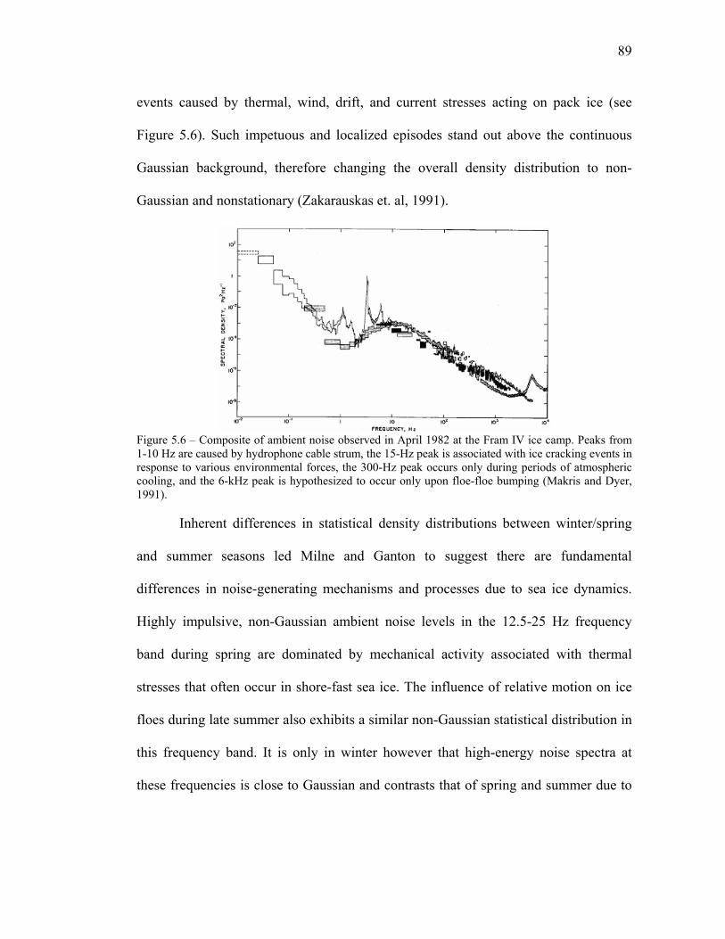
89

events caused by thermal, wind, drift, and current stresses acting on pack ice (see

Figure 5.6). Such impetuous and localized episodes stand out above the continuous

Gaussian background, therefore changing the overall density distribution to non-

Gaussian and nonstationary (Zakarauskas et. al, 1991).

Figure 5.6 – Composite of ambient noise observed in April 1982 at the Fram IV ice camp. Peaks from 1-10 Hz are caused by hydrophone cable strum, the 15-Hz peak is associated with ice cracking events in response to various environmental forces, the 300-Hz peak occurs only during periods of atmospheric cooling, and the 6-kHz peak is hypothesized to occur only upon floe-floe bumping (Makris and Dyer, 1991). Inherent differences in statistical density distributions between winter/spring

and summer seasons led Milne and Ganton to suggest there are fundamental

differences in noise-generating mechanisms and processes due to sea ice dynamics.

Highly impulsive, non-Gaussian ambient noise levels in the 12.5-25 Hz frequency

band during spring are dominated by mechanical activity associated with thermal

stresses that often occur in shore-fast sea ice. The influence of relative motion on ice

floes during late summer also exhibits a similar non-Gaussian statistical distribution in

this frequency band. It is only in winter however that high-energy noise spectra at

these frequencies is close to Gaussian and contrasts that of spring and summer due to

90

fully-hardened ice coverage. The absence of impulsive noise in the 200-400 Hz band

reveals a near-Gaussian spectral distribution during summer in contrast to that of

springtime, while the 3.2-6.4 kHz band is impulsive and therefore non-Gaussian

during summer in contrast to a Gaussian distribution in spring (Milne and Ganton,

1964).

The non-Gaussian nature of thermally induced impulsive noise is characterized

by a spectral-energy peak between 100-400 Hz with a slope of -12 dB/octave at higher

frequencies (see Figure 5.7). Milne and Ganton observed that a profusion of localized

thermal fracturing accounted for a near-normal Gaussian statistical density distribution

for ambient noise spectra above 1 kHz when derived from a superposition of these

impulsive acoustic events. They also noticed though that the frequency band between

100 Hz and 10 kHz exhibited spectral levels that could either decrease as a function of

logarithmically increasing frequency or were entirely frequency independent. Because

of sea ice cover, spectrum levels for wind-generated noise were usually Gaussian in

nature and essentially frequency independent between 100 Hz and 10 kHz (Milne and

Ganton, 1964).

Figure 5.7 – Power spectrum levels in third-octave bands of three ambient noise samples (Zakarauskas et. al, 1991).

91

Implications for Arctic Marine Mammal Research

Long-term continuously recorded acoustic data from the coastal Arctic Ocean

can provide an effective tool for studying aspects of marine mammal populations that

are difficult or impossile to study using other methods of observation. Intra-annual

variability in calling behavior of three species was readily assessed, showing the

strong seasonal signal expected for animals whose distribution is closely tied to the

extent and state of sea ice. By overwintering the instruments under 100% ice cover,

aspects of ice seal distribution and behavior that had not been previously recorded

were observed; sporadic events like the appearance of a calling bowhead whale in

January were detected. There were also several unidentified biological calls recorded.

Further investigation may show the presence of rarer ice seal species in this region,

like ribbon and spotted seals.

The 2006 data from the two HARPs deployed north of Barrow will provide an

important baseline for future comparisons of the distribution and seasonal behavior of

marine mammals in the western Arctic. For example, multi-year comparisons will

make it possible to infer whether ice seals are shifting closer to or farther away from

the coast during the winter or spring seasons, or whether formerly uncommon or rare

species are moving into the study area. Correlation with the environmental variables of

ice cover and wind may help to explain some of these changes. Furthermore, male

bearded seals typically produce calls during the breeding season from April to July,

but all four types of mating calls were recorded as early as December. While it is not

possible to determine if this is typical due to a lack of previous recordings during

92

winter months, a time series of year-long recordings spanning multiple years should

help to shed light on trends, if any exist, in the timing of mating behavior of this

species.

Another example of the value of multi-year comparisons of biological

detections in this region is the gray whale, not treated in this analysis. It is important to

note that although historically uncommon in this region of the Arctic, gray whale

sightings have increased over the past decade and calls were recorded throughout the

winter during a 2003 long-term deployment of three previous-generation HARPs in

the Beaufort Sea to the southwest (Stafford et al. 2007). This implies that significant

changes in the distribution of this species may be underway. It will be possible to

study this by recording year-round continuous acoustic data.

Autonomous acoustic recording can be used reliably to confirm the presence of

marine mammal species within some radius of detection from the instrument

locations. For this reason, long-term acoustic recording can provide an effective tool

for monitoring changes in the distribution of marine mammal species over time as

changes in sea ice and other environmental conditions cause shifts in the ecological

regimes of the Arctic. Current limitations of autonomous long-term recording are that,

while presence of a species can be confirmed from call detections, species abundance

can not be infered from calling rates. Furthermore, species absence can not be

confirmed by acoustic methods alone when calls are not present, due to variations in

calling behavior (Stirling 1983, Van Parijs 2001). One special exception to some of

the limitations in the area of more detailed population studies may be the bearded seal.

93

Vocalizations of male bearded seals north of Point Barrow have shown individual

characteristics that have remained stable on decadal time scales (Van Parijs 2006). By

providing an acoustic proxy for traditional mark recapture methods, this opens up the

possibility to study demographic and behavioral aspects of marine mammal

populations.

94

VI. CONCLUSION

Combined with ancillary measurements, long-term acoustic monitoring

provides an effective tool for observing changing levels of ambient sound related to

declining sea ice, environmental mechanisms, and man-made noise, while

simultaneously detecting marine mammals. Acoustic baseline measurments over the

next several years are needed for further analysis in order to observe and compare

shifts in ambient noise due to the current trends in sea ice decline and increases in

anthropogenic noise. Continuing the long-term acoustic data time series at monitoring

sites around the North Slope will facilitate inter-comparison to reveal shifts in

seasonal trends. The critical timing of this study is substantiated by the time-variant

impact of sea ice decline due to the advent of climate change in polar regions.

A particularly interesting facet contained in the first-year dataset is being

explored as a separate study. There is much potential for accurate development of an

acoustic-source propagation model for seismic airgun activity – based on modal

dispersion data collected by the hydrophone – used in conjunction with survey track

lines from 2006. This will help to investigate the possibility of potential impact on

bowhead behavior by providing estimates of received sound-pressure levels that

animals are exposed to, based on the amount of energy transmitted from the seismic

source and the dispersion characteristics associated with attenuation across the

waveguide. Bowheads are a crucial species to consider because of the frequency band

in which they call overlaps with the band containing residual seismic energy.

95

New and better hardware is needed, most importantly: (1) increasing

hydrophone sensitivity at high-frequencies; (2) switching to lithium batteries in order

to achieve a full year of autonomous data recording capability; (3) simaltaneously

deploying upward-looking sonar profilers to explore the complex relationship between

sea ice thickness and associated ambient noise levels; (4) developing shallow-water

mooring configurations that are safe from ice scours and can be deployed near the

coast to monitor marine mammal populations. These improvements will not only

increase acoustic recording capability, but will allow for new avenues in signal

processing and data analysis.

Social implications for acoustics in a seasonal Arctic include increases in

ambient noise levels across the North Slope of Alaska, due in significant part to

anthropogenic noise sources like seismic oil exploration, eventual oil and gas

extraction, maritime shipping activites and vessel traffic, and possible consequences

for marine mammals and the subsistence hunting culture of the North Slope.

96

REFERENCES Albers, V. M., “Underwater Acoustics Handbook II,” University Park, Pennsylvania

State University Press (1965). Bel’kovitch, V. M. and M. N. Sh’ekotov, “The Belukha Whale: Natural Behavior and

Bioacoustics,” Translated by M. A. Svanidze, Edited by J. C. Haney and C. Recchia, Woods Hole Oceanographic Institution (1993).

Buck, B. M., “Arctic Acoustic Transmission Loss and Ambient Noise,” Arctic

Drifting Stations, A Report on Activities Supported by the Office of Naval Research, The Arctic Institute of North America, coordinated by J. E. Sater (1968).

Buck, B. M. and C. R. Green, “Arctic Deep Water Propagation Measurements,” J.

Acoust. Soc. Am. Vol. 36, pp. 1526-1533 (1964). Clark, C. W., R. A. Charif, S. G. Mitchell, J. Colby, “Distribution and behavior of the

bowhead whale, Balaena Mysticetus, based on analysis of acoustic data collected during the 1993 spring migration off Point Barrow, Alaska,” Scientific Report, International Whaling Comission 46: 541-552 (1996).

Diachok, O. I., “Arctic Hydroacoustics,” Cold Regions Sci. Tech. Vol. 2, pp. 299-321

(1980).

Diachok, O. I., “Effects of Sea-Ice Ridges on Sound Propagation in the Arctic Ocean,” J. Acoust. Soc. Am. Vol. 59, No. 5, pp. 1110-1120 (1976).

Diachok, O. I. and R. S. Winokur, “Spatial Variability of Underwater Ambient Noise

at the Arctic Ice-Water Boundary,” J. Acoust. Soc. Am. Vol. 55, No. 4, pp. 750-753 (1974).

Dyer, I., “Statistics of Sound Propagation in the Ocean,” J. Acoust. Soc. Am. Vol. 48,

No. 1 (Part 2) (1970).

Dyer, I., “The Song of Sea Ice and Other Arctic Ocean Melodies,” Arctic Technology and Policy, edited by I. Dyer and C. Chryssostomidis, McGraw-Hill, New York, pp. 11-37 (1984).

Emery, W. J. and R. E. Thomson, “Data Analysis Methods in Physical Oceanography”

2nd edition, Pergamon Press, Amsterdam, 634 pp (1998).

Foldy, L. L., “The Multiple Scattering of Waves: General Theory of Isotropic Scattering by Randomly Distributed Scatterers,” Physical Review Vol. 67, No. 3 & 4, pp. 107-119 (1945).

97

Ganton, J. H. and A. R. Milne, “Temperature and Wind-Dependent Ambient Noise

Under Midwinter Pack Ice” J. Acoust Soc. Am. Vol. 38, pp. 406-411 (1965).

Green, C. R. and B. M. Buck, “Arctic Ocean Ambient Noise,” J. Acoust. Soc. Am. Vol. 36, pp. 1218-1220 (1964).

Kahru, M., “Windows Image Manager—Image display and analysis program for

Microsoft Windows with special features for satellite images,” WWW page, http://wimsoft.com (2000).

Kaufman, M., “Perennial Arctic Ice Cover Diminishing, Officials Say,” Washington

Post, Pg. A03 (March 19, 2008).

Kibblewhite, A. C. and D. A. Jones, “Ambient Noise Under Antarctic Sea Ice,” J. Acoust. Soc. Am. Vol. 59, No. 4 (1976).

LePage, K. and H. Schmidt, “Modeling of Low-frequency Transmission Loss in the

Central Arctic,” J. Acoust. Soc. Am. Vol. 96, No. 3 (1994).

Lewis, J. K. and W. W. Denner, “A Study of Sea Ice Kinematics and Their Relationships to Arctic Ambient Noise,” Report to the Office of Naval Research, Science Applications International Corporation Report No. SAIC 85/1950, pp. 770 (1986).

Lewis, J. K. and W. W. Denner, “Arctic Ambient Noise in the Beaufort Sea: Seasonal

Relationships to Sea Ice Kinematics,” J. Acoust. Soc. Am. Vo1. 83, No.2, pp. 549-565 (1988).

Lewis, J. K. and W. W. Denner, “Arctic Ambient Noise in the Beaufort Sea: Seasonal

Space and Time Scales,” J. Acoust. Soc. Am. Vo1.82, No.3, pp. 988-997 (1987).

Lewis, J. K. and W. W. Denner, “Higher Frequency Ambient Noise in the Arctic Ocean,” J. Acoust. Soc. Am. Vol. 84, No. 4, pp. 1444-1455 (1988).

Mackenzie, K. V., “Nine-term equation for sound speed in the oceans,” J. Acoust. Soc.

Am. Vol. 70, No. 3 (1981). MacPherson, J. D., “Some Under-Ice Acoustic Ambient Noise Measurements,” J.

Acoust. Soc. Am. Vol. 34 (L), pp. 1149-1150 (1962).

Makris, N. C. and I. Dyer, “Environmental Correlates of Arctic Ice Edge Noise,” J. Acoust. Soc. Am. Vol. 90, No. 6 (1991).

98

Makris, N. C. and I. Dyer, “Environmental Correlates of Pack Ice Noise,” J. Acoust. Soc. Am. Vol. 79, No. 5, pp. 1434-1440 (1986).

McDonald, M. A., J. A. Hildebrand, S. M. Wiggins, “Increases in deep ocean ambient

noise in the Northeast Pacific west of San Nicolas Island, California,” J. Acoust. Soc. Am. Vol. 120, No. 2, pp. 711-718 (2006).

Milne, A. R., “Sound Propagation and Ambient Noise Under Sea Ice,” in Underwater

Acoustics, edited by V. M. Albers (Plenum, New York), Vol. 2, Ch. 7, pp. 103-137 (1967).

Milne, A. R., “Statistical Description of Noise Under Shore-Fast Sea Ice in Winter,” J.

Acoust. Soc. Am. Vol. 39, pp. 1174-1182 (1966)

Milne, A. R., “Thermal Tension Cracking in Sea Ice: A Source of Under Ice Noise,” J. Geophysics Res. Vol. 77, pp. 2177-2192 (1972).

Milne, A. R., “Wind Noise Under Winter Ice Fields,” J. Geophysics Res. Vol. 79, pp.

803-809 (1974).

Milne, A. R. and J. H. Ganton, “A Statistical Description of Noise Under Shore-Fast Sea-Ice in Winter,” Pacific Naval Lab. Report 65-1 (1965).

Milne, A. R. and J. H. Ganton, “Ambient Noise Under Arctic Sea Ice,” J. Acoust. Soc.

Am. Vol. 36, No. 5, pp. 855-863 (1964). Milne, A. R. and J. H. Ganton, “Diurnal Variations in Underwater Noise Beneath

Spring-Time Sea Ice,” Nature Vol. 221, pp. 851-852 (1969).

Milne, A. R. and J. H. Ganton, “Noise Beneath Sea Ice and its Dependence on Environmental Mechanisms,” JUA (USN) Vol. 21, pp. 69-81 (1971).

Milne, A. R., J. H. Ganton, and D. J. McMillin, “Ambient Noise Under Sea Ice and

Further Measurements of Wind and Temperature Dependence,” J. Acoust. Soc. Am. Vol. 41 (L), pp. 525-528 (1967).

Moore, S. E., K. M. Stafford, D. K. Mellinger, J. A. Hildebrand, “Listening for Large

Whales in the Offshore Waters of Alaska,” Bioscience Vol. 56, No. 1, pp. 49-55 (2006).

Payne, F. A., “Effect of Ice Cover on Shallow-Water Ambient Sea Noise,” J. Acoust.

Soc. Am. Vol. 36, pp. 1943-1947 (1964).

99

Pritchard, R. S., “Arctic Ocean Background Noise Caused by Ridging of Sea Ice” J. Acoust. Soc. Am. Vol. 75, No. 2 (1984).

Pritchard, R. S., “Mechanical Behavior of Pack Ice,” in Mechanics of Structured

Media, edited by A.P.S. Selvadurai (Elsevier, Amsterdam), pp. 371-405 (1981). Risch, D., C. W. Clark, P. J. Corkeron, A. Elepfandt, K. M. Kovacs, C. Lydersen, I.

Stirling, S. M. Van Parijs, “Vocalizations of male bearded seals, Erignathus barbatus: classification and geographical variation,” Animal Behaviour, Vol. 73, No. 5, pp. 747-762 (2007).

Ross, D., “Mechanics of Underwater Noise,” Pergamon, New York, p. 375 (1976). Spreen, G., L. Kaleschke, G. Heygster, “AMSR-E ASI 6.25 km Sea Ice Concentration

Data, V5.2,” Institute of Environmental Physics, University of Bremen, Germany, digital media: www.iup.physik.uni-bremen.de (2008).

Spreen, G., L. Kaleschke, G. Heygster, “Sea Ice Remote Sensing Using AMSR-E 89-

GHz Channels,” J. Geophys. Res. Vol. 113, C02S03 (2008).

Squire, V., J. Dugan, P. Wadhams, P. Rottier, A. Liu, “Of Ocean Waves and Sea Ice,” Annu. Rev. Fluid Mech. Vol. 27, pp. 115-168 (1995).

Stafford, K. M., S. E. Moore, M. Spillane, S. M. Wiggins, “Gray whale calls recorded

near Barrow, Alaska, throughout the winter of 2003-04,” Arctic, Vol. 60, pp. 167 (2007).

Stirling, I., W. Calvert, H. Cleator, “Underwater Vocalizations as a Tool for Studying

the Distribution and Relative Abundance of Wintering Pinnipeds in the High Arctic,” Arctic, Vol. 36, No. 3, pp. 262-274 (1983).

Stroeve, J., M. M. Holland, W. Meier, T. Scambos, M. Serreze, “Arctic Sea Ice

Decline: Faster than Forecast,” Geophysical Research Letters, Vol. 34, L09501 (2007).

Suydam, R. S., L. F. Lowry, K. J. Frost, G. M. O’Corry-Crowe, D. Pikok, “Satellite

Tracking of Eastern Chukchi Sea Beluga Whales into the Arctic Ocean,” Arctic, Vol. 54, No. 3, pp. 237-243 (2001).

Van Parijs, S. M., K. M. Kovacs, C. Lydersen, “Spatial and Temporal Distribution of Vocalizing Male Bearded Seals – Implications for Male Mating Strategies,” Behaviour, Vol. 138, pp. 905-922 (2001).

100

Van Parijs, S. M., C. W. Clark, “Long-term mating tactics in an aquatic-mating pinniped, the bearded seal, Erignathus barbatus,” Animal Behaviour, Vol. 72, No. 6, pp. 1269-1277 (2006).

Webb, S. C. and A. Schultz, “Very Low Frequency Ambient Noise at the Seafloor

Under the Beaufort Sea Icecap,” J. Acoust. Soc. Am. Vol. 91, No. 3 (1992).

Welch, P., “The use of fast Fourier transform for the estimation of power spectra: A method based on time averaging over short, modified periodograms,” IEEE Transactions on Audio and Electroacoustics, Vol. 15, Issue 2, pp. 70-73 (1967).

Wenz, G. M., “Acoustic Ambient Noise in the Ocean: Spectra and Sources,” J.

Acoust. Soc. Am. Vol. 34, No. 12, pp. 1936-1956 (1962).

Wiggins, S. M., “Autonomous Acoustic Recording Packages (ARPs) for Long-Term Monitoring of Whale Sounds,” MTS Journal, Vol. 37, No. 2, pp. 13-22 (2003).

Wiggins, S. M. and J. A. Hildebrand, “High-frequency Acoustic Recording Package

(HARP) for Broad-band, Long-term Marine Mammal Monitoring,” Symposium on Underwater Technology and Workshop on Scientific Use of Submarine Cables and Related Technologies, pp. 551-557 (2007).

Yang, T. C. and C. W. Votaw, “Under Ice Reflectivities at Frequencies Below 1 kHz,”

J. Acoust. Soc. Am. Vol. 70, No. 3 (1981).

Zakarauskas, P., “Observation of Thermal Ice Cracking in the Arctic Basin,” J. Acoust. Soc. Am. Suppl. 1, Vol. 82, No. S30 (1987).

Zakarauskas, P., C. J. Parfitt, J. M. Thorleifson, “Automatic Extraction of Spring-

Time Arctic Ambient Noise Transients,” J. Acoust. Soc. Am. Vol. 90, No. 1 (1991).