SUPPORTING INFORMATION

Spatial variations of methane emission in a large and shallow eutrophic lake in subtropical climate

Qitao Xiao1, Mi Zhang1, *, Zhenghua Hu1, Yunqiu Gao1, Cheng Hu1, Cheng Liu1, Shoudong Liu1, Zhen Zhang1, Jiayu Zhao1, Wei Xiao1, X Lee1,2, *

Contents:

Figure S1. Effects of storage time on dissolved methane concentration.

Figure S2. Effects of headspace fraction on dissolved methane concentration.

Figure S3. A diel composite of pH in surface water.

Figure S4. Temporal variation of the surface dissolved CH4.

Figure S5. Temporal variation of wind speed.

Figure S6. Diel variation of the diffusion CH4 flux at MLW.

Table S1. Annual mean total phosphorous (TP) and total nitrogen (TN) of the seven zones in Lake Taihu in 2014.

Table S2. Temporal correlation of the diffusion CH4 flux with wind speed and dissolved CH4 concentration.

Table S3. Pearson correlation between these explanatory environmental variables.

Table S4. VIF and AIC values for multiple linear regressions.

Supplementary text regarding comparison of the gas transfer coefficient k calculated by four different models

Figure S7. Comparison of the diffusion CH4 flux calculated with four different models of the gas transfer coefficient.

1

1

2

3

45

6

789

1011

1213

1415

1617

1819

2021

2223

242526

272829

3031

3233

343536

37

38

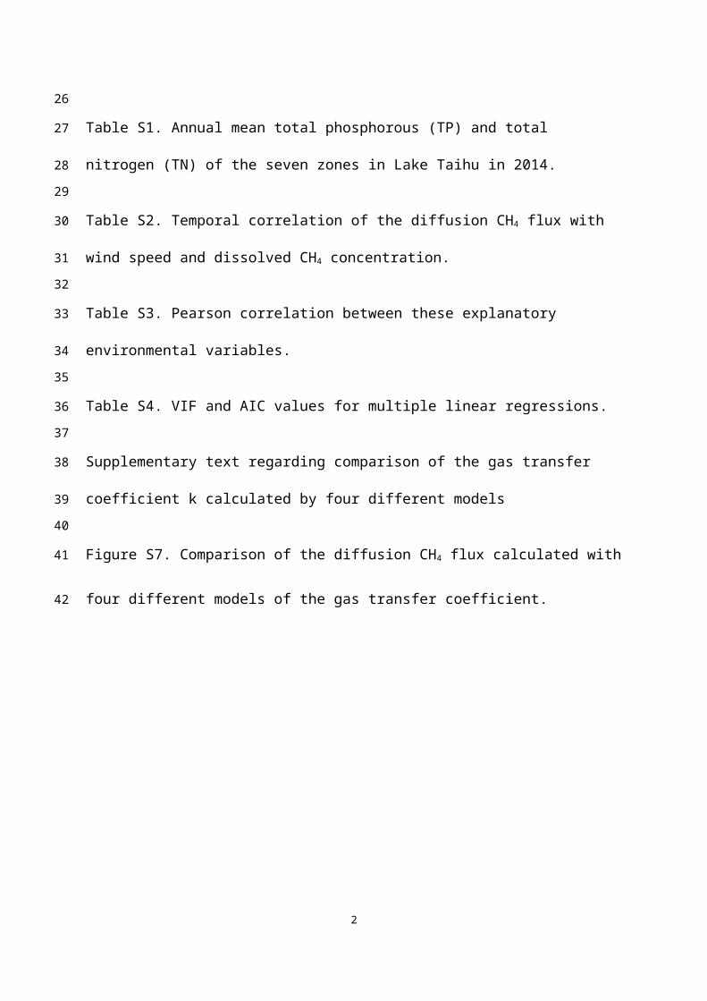
Figure S1. Effects of storage time on the dissolved methane concentration using water samples collected at BFG (a) and MLW (b). Each treatment was replicated three times. Error bars are one standard deviation. CTRL: measurement was made without delay. NS: difference from CNTRL is not statistically significant.

2

3940414243

44

Figure S2. Effects of headspace fraction on the dissolved methane concentration using water samples collected at a local pond (a) and at MLW (b). Each treatment was replicated three times. Error bars are one standard deviation.

3

454647

48

49

Figure S3. A diel composite of pH observed at the 20-cm depth at a buoy site in Gonghu Bay (location labeled as SSC in the map inset). Observations were made over 155 days in the summer of 2009 and in the winter of 2009-2010 (Hu et al., 2015).

4

505152

53

Figure S4. Temporal variation of the surface dissolved CH4 at the five lake observation sites (MLW, BFG, DPK, XLS, and PTS) where frequent water sampling took place. Their locations are shown in Figure 1. Red circles indicate the whole-lake mean dissolved CH4 concentration. The error bar is ±1 standard deviation.

5

54555657

5859

Figure S5. Temporal variation of wind speed at the five lake observation sites (MLW, BFG, DPK, XLS, and PTS) where frequent water sampling took place. Their locations are shown in Figure 1.

6

606162

63

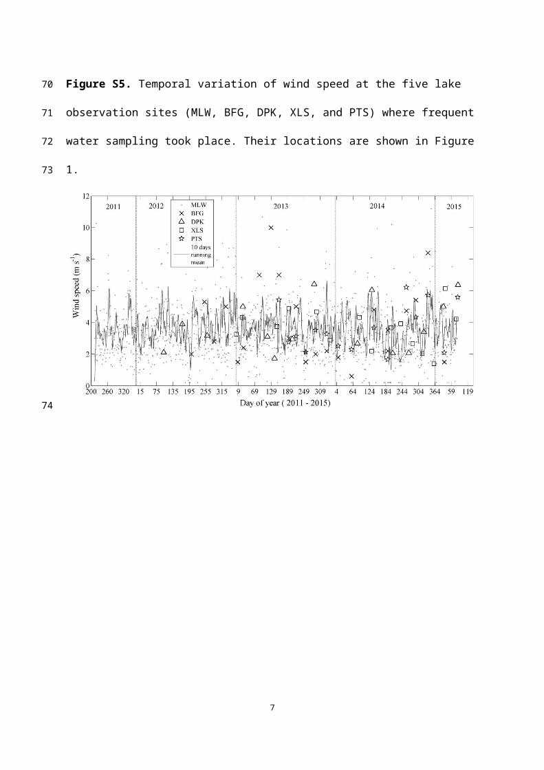
Figure S6. Diel variation of the diffusion CH4 flux at MLW. The gas transfer coefficient was determined with the model described by Cole et al. (1998, a), and with a model that considers both wind speed and waterside convection (Podgrajsek et al., 2015, b). Error bars are ± 1 standard error.

7

64656667

68

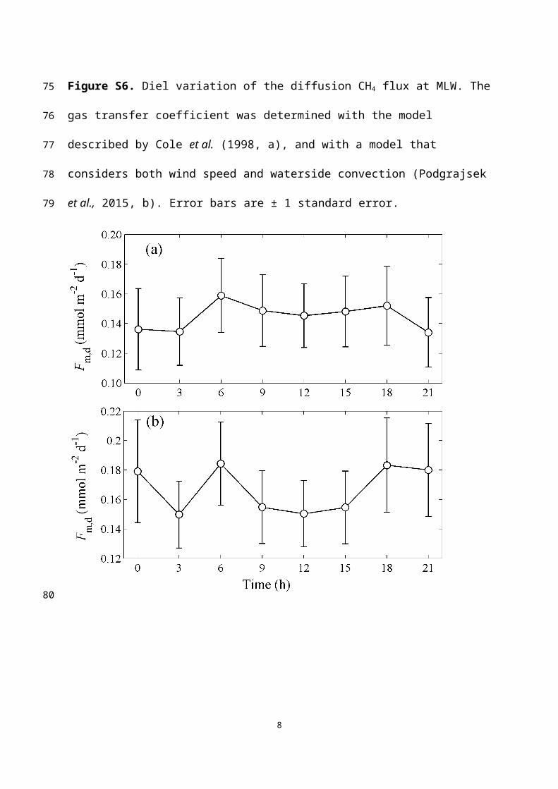
Table S1. Annual mean total phosphorous (TP) and total nitrogen (TN) of the seven zones in Lake Taihu in 2014.

Zones Area (km2) TP (mg L-1) TN ( mg L-1) Trophic class1

Meiliang Bay 100 0.087 2.18 Eutrophic

Gonghu Bay 215.6 0.065 1.81 Mesotrophic

East Zone 316.4 0.033 1.23 Mesotrophic

Dongtaihu Bay 131 0.037 0.90 Mesotrophic

Southwest Zone 443.2 0.067 2.01 Mesotrophic

Northwest Zone 394.1 0.094 2.58 Hyper-eutrophic

Central Zone 737.5 0.072 1.89 Mesotrophic

Whole lake 2338 0.069 1.90 Eutrophic

Data source: The Health Status Report of Taihu Lake, Taihu Basin Authority of Ministry of Water Resources and Electric Power, http://www.tba.gov.cn/.

1: Trophic classifications are defined according to OECD (Organization for Economic Cooperation and Development) (1982), Eutrophication of Waters. Monitoring assessment and control. Final Report. OECD Cooperative Programme on Monitoring of Inland Waters (Eutrophication Control), Environment Directorate, OECD, Paris.

8

6970

717273

74757677

Table S2. Temporal correlation of the diffusion CH4 flux (mmol m-2 d-1) with wind speed (m s-1) and dissolved CH4 concentration (nmol L-1) at five locations (MLW, BFG, DPK, XLS, and PTS).

Site CH4 concentration Wind speed

MLWy = 0.0011x – 0.0193

R = 0.92 p < 0.001 n = 1261

y = 0.0934x – 0.1852

R = 0.09 p < 0.001 n = 1264

BFGy = 0.0015x – 0.0468

R = 0.84 p < 0.001 n = 24

y = 0.0514x – 0.0601

R = 0.21 p = 0.315 n = 24

DPKy = 0.0010x – 0.0032

R = 0.93 p < 0.001 n = 15

y = -0.0255x +0.1470

R = -0.21 p = 0.458 n = 15

XLSy = 0.0016x – 0.0164

R = 0.97 p < 0.001 n = 15

y = 0.0276x – 0.0688

R = 0.33 p = 0.223 n = 15

PTSy = 0.0010x – 0.0028

R = 0.94 p < 0.001 n = 15

y = 0.0114x – 0.0232

R = 0.13 p = 0.654 n = 15

9

78

79808182

8384

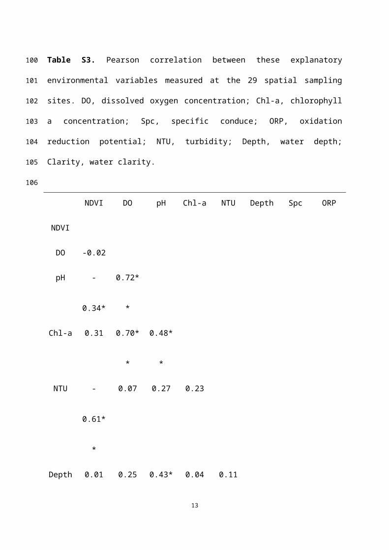
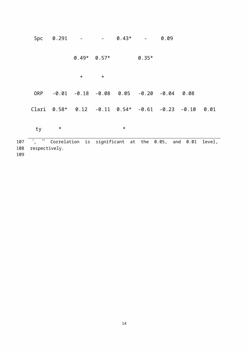
Table S3. Pearson correlation between these explanatory environmental variables measured at the 29 spatial sampling sites. DO, dissolved oxygen concentration; Chl-a, chlorophyll a concentration; Spc, specific conduce; ORP, oxidation reduction potential; NTU, turbidity; Depth, water depth; Clarity, water clarity.

NDVI DO pH Chl-a NTU Depth Spc ORP

NDVI

DO -0.02

pH -0.34* 0.72**

Chl-a 0.31 0.70** 0.48**

NTU -0.61** 0.07 0.27 0.23

Depth 0.01 0.25 0.43* 0.04 0.11

Spc 0.291 -0.49** -0.57** 0.43* -0.35* 0.09

ORP -0.01 -0.18 -0.08 0.05 -0.20 -0.04 0.08

Clarity 0.58** 0.12 -0.11 0.54** -0.61 -0.23 -0.10 0.01*, ** Correlation is significant at the 0.05, and 0.01 level, respectively.

10

8586878889

9091

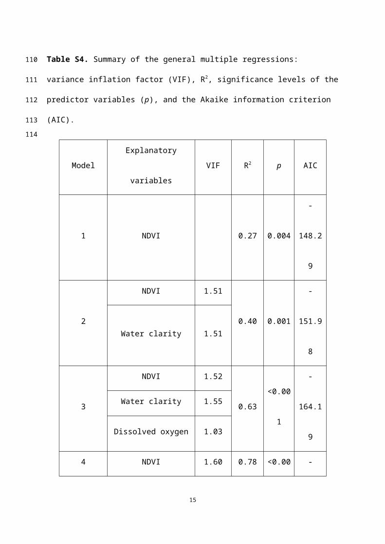
Table S4. Summary of the general multiple regressions: variance inflation factor (VIF), R2, significance levels of the predictor variables (p), and the Akaike information criterion (AIC).

Model Explanatory variables VIF R2 p AIC

1 NDVI 0.27 0.004 -148.29

2NDVI 1.51

0.40 0.001 -151.98Water clarity 1.51

3

NDVI 1.52

0.63 <0.001 -164.19Water clarity 1.55

Dissolved oxygen 1.03

4

NDVI 1.60

0.78 <0.001 -176.46Water clarity 1.75

Dissolved oxygen 1.14

Water depth 1.21

11

929394

95

Comparison of the diffusion flux calculated with four different models for the gas

transfer coefficient

In this supplementary section, we present a comparison of the diffusion flux calculated using

four different models for the gas transfer coefficient. The four models are described by Cole

et al. (1998, k1), Read et al. (2012, k2), Heiskanen et al. (2014, k3), and Podgrajsek et al.

(2015, k4).

The first model is that of Cole et al. (1998). In this model, the gas transfer coefficient k1 is

wind-dependent and is normalized to a Schmidt number 600 of a gas at temperature of 20 oC,

k1 = k600 × (Sc/600)-n (S1)

where Sc is Schmidt number for CH4 at in-situ temperature. For the exponent n, we used the

value 2/3 at low wind speed (U10 < 3.7 m s-1) according to Huotari et al. (2009) and the value

of 1/2 at high wind speed (U10 > 3.7 m s-1) according to MacIntyre et al. (1995) and Juutinen

et al. (2009). An empirical relationship was used to determine k600 (cm h-1; Cole and Caraco,

1998):

k600 = 2.07 + 0.215U 101.7 (S2)

where U10 is wind speed at the 10-m height (m s-1). The required input is U10, which was

measured by a wind sensor at PTS in the lake.

The second model is a surface renewal scheme described Read et al. (2012). It considers both

wind shear (εu) and waterside convection (εw),

k2 = η(εν)0.25Sc-n (S3)

12

96

97

98

99

100

101

102

103

104

105

106

107

108

109

110

111

112

113

114

115

116

117

where η is a proportionality constant, ν is the kinematic viscosity of water, n is a coefficient

representing surface conditions, and

ε = εu + εw (S4)

is the turbulent kinetic energy dissipation rate representing the total contribution from wind

shear (εu) and waterside convection (εw). The wind shear contribution is given by

εu = (τt/ρw)/(Κδv) (S5)

where τt is the tangential shear stress in air, ρw is the density of water, K is the von Karman

constant, and δv is the thickness of the viscous sublayer given by Soloviev et al. (2007),

δv = c1ν/(τt /ρw)0.5 (S6)

where c1 is a dimensionless constant.

The contribution by waterside convection (εw) is given as,

εw = -β (S7)

where β is buoyancy flux defined as

β = ga Qe

ρw Cp

(S8)

where g is the acceleration of gravity, a is the thermal expansion coefficient of water, Cp is

the specific heat of water, Qe is the effective surface heat flux (Imberger, 1985; Jeffery et al.,

2007). If the lake is gaining heat from the atmosphere (Qe > 0), εw is set to zero.

We used the air friction velocity measured at PTS to determine τt in Equation S5 and S6, and

approximate the surface heat flux Qe as the residual of the surface energy balance equation,

Qe = Rn – H – λE (S9)

13

118

119

120

121

122

123

124

125

126

127

128

129

130

131

132

133

134

135

136

137

138

where Rn (net radiation), H (sensible heat flux), and λE (latent heat flux) were measured at

PTS. Other coefficients are given by Read et al. (2012) as η= 0.29, n = 0.5, and Sc = 600.

The third model, described by MacIntyre et al. (2010) and Heiskanen et al. (2014), is also a

surface renewal parameterization. It uses different fitting coefficients from Read et al. (2012)

to calculate the gas transfer coefficient,

k3 = 0.5(εν)0.25Sc-n (S10)

ε = 0.77 (-β) + 0.3 (uw¿ )3/(Kz) (S11)

where β is buoyancy flux defined by Equation S8, z is a mixed layer depth, uw¿ is the velocity

scale for wind shear given by

uw¿ = ua

¿ √ ρa

ρw

(S12)

where ρa is the density of air, ua¿ is the air friction velocity measured at PTS in the lake,

Sc is the Schmidt number for CH4 at in-situ temperature, n = 0.5, and the mixing layer depth z

was set to 0.5 m according to the thermal diffusivity profile calculated with the model of

Herb and Stephan (2005) for Lake Taihu.

The fourth model is that of Podgrajsek et al. (2015) which also considers the effect of

waterside convection. The gas transfer coefficient k4 is given as

k4 = k1 + 0.05 × exp(1068 × (β z)1/3) (S13)

where k1is determined by Equation S1, β is defined by Equation S8, and z is the mixed layer

14

139

140

141

142

143

144

145

146

147

148

149

150

151

152

153

154

155

156

157

158

depth. In this equation, the second term represents the contribution of waterside convection to

the gas transfer.

We estimated the percentage of the gas transfer (kw) driven by waterside convection from the

last three models. In the case of the second model, kw was computed from Equation S3 by

setting εu to zero. In the third and the fourth model, kw was computed from Equation S10 and

S13 by setting uw¿ and k1 to zero, respectively. The percent of the contribution of waterside

convection is

kw%= (kw/k)100% (S14)

where k is the total gas transfer coefficient driven by wind shear and waterside

convection.

Figure S7 compares the annual mean diffusion flux from the four models. The annual mean

CH4 diffusion fluxes based on the four different diffusivity formulations were 0.092 (Cole et

al., 1998), 0.103 (Read et al., 2012), 0.080 (Heiskanen et al., 2014), and 0.093 mmol m-2 d-1

(Podgrajsek et al., 2015).

15

159

160

161

162

163

164

165

166

167

168

169

170

171

172

173

174

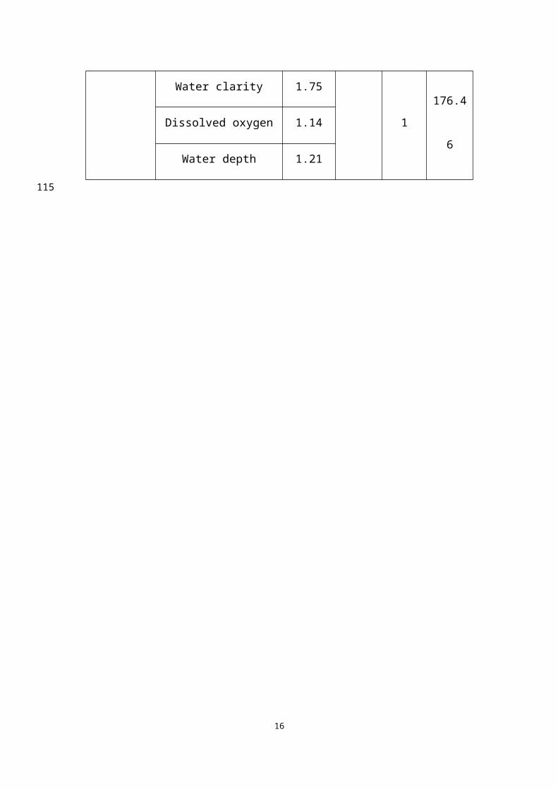
Figure S7. Comparison of the whole-lake diffusion CH4 flux calculated with four different models of the gas transfer coefficient. Error bars are one standard deviation of the12 annual mean values for the 29 lake survey locations (Figure 1).

16

175176177

178179

References

Cole, J. J., and N. F. Caraco (1998), Atmospheric exchange of carbon dioxide in a low-wind oligotrophic lake measured by the addition of SF6, Limnol. Oceanogr., 43(4), 647-656.

Heiskanen, J., I. Mammarella, S. Haapanala, J. Pumpanen, T. Vesala, S. MacInytre, A. Ojala (2014), Effects of cooling and internal wave motions on gas transfer coefficients in a boreal lake, Tellus B, 66, doi: 10.3402/tellusb.v66.22827.

Herb, W. R., H. G. Stefan (2005), Dynamics of vertical mixing in a shallow lake with submersed macrophytes, Water Resour. Res., 41, W02023, doi:10.1029/2003WR002613

Huotari, J., Ojala, A., Peltomaa, E., et al., (2009), Temporal variation in surface water CO2 concentration in a boreal humic lake based on high-frequency measurement, Boreal Env. Res. ,14(Suppl. A): 48-60.

Imberger, J. (1985), The diurnal mixed layer, Limnol. Oceanogr., 30(4), 737-770, doi:10.4319/lo.1985.30.4.0737.

Jeffery, C. D., D. K. Woolf, I. S. Robinson, and C. J. Donlon (2007), One-dimensional modeling of convective CO2 exchange in the tropical Atlantic, Ocean Model., 19(3–4), 161-182, doi:10.1016/j.ocemod.2007.07.003.

Juutinen, S., M. Rantakari, P. Kortelainen, J. T. Huttunen, T. Larmola1, J. Alm, J. Silvola, and P. J. Martikainen, (2009), Methane dynamics in different boreal lake types, Biogeosciences, 6, 209-223.

MacIntyre, S., A. Jonsson, M. Jansson, J. Aberg, D. E. Turney, and S. D. Miller (2010), Buoyancy flux, turbulence, and the gas transfer coefficient in a stratified lake, Geophys. Res. Lett., 37, L24604, doi:10.1029/2010GL044164.

MacIntyre, S., R.Wanninkof, and J. P. Chanton (1995), Trace gas exchange across the air-water interface in freshwater and coastal marine environments, in, edited by: Matson, P. A. and Harriss, R. C., Biogenic trace gases: Measuring emissions from soil and water. Methods in ecology, 52-97, Blackwell Science.

Podgrajsek, E., E. Sahlée, and A. Rutgersson (2015), Diel cycle of lake-air CO2 flux from a shallow lake and the impact of waterside convection on the transfer velocity, J. Geophys. Res. Biogeosci., 120, 29–38, doi:10.1002/2014JG002781. Read, J. S., et al. (2012), Lake-size dependency of wind shear and convection as controls on gas exchange, Geophys. Res. Lett., 39(9), doi:10.1029/2012gl051886.

Soloviev, A., M. Donelan, H. Graber, B. Haus, P. Schlüsse (2007), An approach to estimation of near-surface turbulence and CO2 transfer velocity from remote sensing data, J. Marine Syst., 66, 182-194.

17

180

181182183

184185186187

188189190

191192193

194195196

197198199200

201202203

204205206207

208209210211

212213214215216217218

219220221