Embed Size (px)
Citation preview

University of Alberta
Library Release Form
Name of Author: Vinay Kariwala
Title of Thesis: Multi-loop Controller Synthesis and Performance Analysis
Degree: Doctor of Philosophy
Year this Degree Granted: 2004
Permission is hereby granted to the University of Alberta Library to reproduce copies of thisthesis and to lend or sell such copies for private, scholarly or scientific research purposesonly.
The author reserves all other publication and other rights in association with the copyrightin the thesis, and except as hereinbefore provided, neither the thesis nor any substantialportion thereof may be printed or otherwise reproduced in any material form whateverwithout the author’s prior written permission.
. . . . . . . . . . . . . . . . . .Vinay KariwalaCME 536University of AlbertaEdmonton, ABCanada, T6G 2G6
Date: . . . . . . . . .

I simply picked a bunch of flowersand added nothing
but the thread that binds them
-Michel De Montaigne, French writer (1533-1592)
University of Alberta
MULTI -LOOP CONTROLLER SYNTHESIS AND PERFORMANCEANALYSIS
by
Vinay Kariwala
A thesis submitted to the Faculty of Graduate Studies and Research in partial fulfillment ofthe requirements for the degree ofDoctor of Philosophy.
in
Process Control
Department of Chemical and Materials Engineering
Edmonton, AlbertaFall 2004

University of Alberta
Faculty of Graduate Studies and Research
The undersigned certify that they have read, and recommend to the Faculty of GraduateStudies and Research for acceptance, a thesis entitledMulti-loop Controller Synthesisand Performance Analysissubmitted by Vinay Kariwala in partial fulfillment of therequirements for the degree ofDoctor of Philosophy in Process Control.
. . . . . . . . . . . . . . . . . .
Dr. J. Fraser Forbes
. . . . . . . . . . . . . . . . . .
Dr. Edward S. Meadows
. . . . . . . . . . . . . . . . . .
Dr. Horacio J. Marquez
. . . . . . . . . . . . . . . . . .
Dr. Sirish L. Shah
. . . . . . . . . . . . . . . . . .
Dr. Richard D. Braatz
Date: . . . . . . . . .

To my family&
Fraser Forbes, my Ph.D. thesis supervisor

Abstract
Over the past few decades, many algorithms have been proposed for controller design. In
practice, an engineer needs to address the following issues before the actual controller can
be designed: which variables should be measured, controlled and manipulated, and what
links should be made between them. These decisions are often taken heuristically, which
has an adverse effect on the safe and economic operation of the process. In this thesis,
simple yet theoretically sound tools are developed for partitioning of the measurements
and manipulations for control of complex systems.
The task of controller design is much simplified by pre-stabilizing the system using
a subset of variables. Selecting the subset of variables by minimization of the input
energy required for stabilization reduces the likelihood of otherwise destabilizing input
saturation. The achievable input performance for linear systems is characterized and an
iterative method is presented for variable selection. The conventionalµ-interaction measure
is generalized for synthesizing a decentralized stabilizing controller using independent
designs. The decentralized controller is designed based on the optimal block diagonal
approximation of the multivariate system.
For the stabilized system, though use of a single large controller is mathematically
attractive, simpler and smaller controllers are often used in practice for ease of maintenance
and design. Connections between closed loop properties and block relative gain are
presented for partitioning the system based on practical issues like reliability and simplified
tuning. It is shown that establishing the existence of a diagonal controller with integral

action for reliable stabilization is NP-hard.
Once the control structure is established, existing methods can be used for controller
design; however, the closed loop performance can deteriorate with time due to uncertain
dynamics and changing operating conditions. Use of online performance monitoring
tools is necessary to identify significant performance degradation and subsequent remedial
steps. The existing methods are inadequate for performance monitoring of decentralized
controllers and a sub-optimal, but explicit solution to the decentralized minimum variance
benchmark problem is proposed.
The tools presented in this thesis can be used individually or synthesized into a
comprehensive design procedure with possible minor extensions.

Acknowledgements
Dr. J. Fraser Forbes is one of the most wonderful persons, I have known. I always wondered
where does he find all the time and energy for his administrative duties and yet be available
to provide advise on technical, as well as non-technical, matters. Fraser allowed me to
venture different terrains on my own, but always made sure that I did not go wayward. Ah!
I am running short of euphemisms. I will always remain indebted to him for his support
and guidance throughout the course of my Ph.D. and hope to continue to benefit from his
experience in the future.
Nothing better could have happened than having Dr. Edward S. Meadows (Scott) as my
co-supervisor. His constant constructive criticism of my work has had a great impact on
the quality of the results presented in this thesis. I will always cherish the memories of
the camping trip and the dinner parties at Scott’s. My cordial acknowledgements to Drs.
Shah, Huang, Chen and Marquez for teaching me the basics of control theory and also for
providing feedback on my research work.
The few months spent in Norway certainly changed the slope of my learning curve
and subsequently the course of this thesis. Thanks to Dr. Skogestad and members of
his research group, Antonio, Vidar, Jens, Marius, Stathis, Espen, Olaf, Hilde for being
such a wonderful host. My acknowledgements to Dr. Shah, Takada san and Douke san
for making the industrial internship in Japan possible. Special thanks to my colleagues
at MCC, Oonedera san, Amano san, Oyama san, Okuda san for taking all the pain in
conversing in the language that I understand and introducing me to delicious soba, udon
and ognomiyaki.
My acknowledgements to Bhushan, Shoukat, Hari, Xin, Mike, Zhengang, Arun and
Liqian for all the discussions. I would also like to thank the department secretaries -

AnnMarie, Judy, Leanne and Showna and the system administrators Jack and Bob. For
whatever social life I had in Edmonton, the credit entirely goes to Hari, Kapil, Venkat,
Errol, Sujit, Arvind, Shakir, Ammul, Sanket, Govind and Mani.
Whenever I was feeling down, my undergraduate friends Pinaki, Chandu, Peeru, Tapan,
Sanju, Jaanu, Pant, Sandy, Khandu and school friends Saurabh and Sushil were always
a call away patiently listening to me cribbing. (Why do people who matter most get
mentioned in the end, probably for emphasis!!). I must acknowledge the love and support
of my family back home in India. To them, this thesis is dedicated.

Contents
1 Introduction 1
1.1 The Case for Decentralized Control. . . . . . . . . . . . . . . . . . . . . 1
1.2 Motivation and Scope. . . . . . . . . . . . . . . . . . . . . . . . . . . . . 2
1.3 Thesis Overview . . . . . . . . . . . . . . . . . . . . . . . . . . . . . . . 4
2 Input Performance Limitations of Feedback Control 7
2.1 Introduction. . . . . . . . . . . . . . . . . . . . . . . . . . . . . . . . . . 7
2.2 Preliminaries . . . . . . . . . . . . . . . . . . . . . . . . . . . . . . . . .10
2.2.1 Poles and Zeros. . . . . . . . . . . . . . . . . . . . . . . . . . . .10
2.2.2 All Pass Factorization of RHP Poles and Zeros. . . . . . . . . . . 11
2.2.3 Optimal Control . . . . . . . . . . . . . . . . . . . . . . . . . . . 12
2.2.4 Hankel Singular Values and Balanced Realization. . . . . . . . . . 14
2.3 Problem Formulation and Simplification. . . . . . . . . . . . . . . . . . . 16
2.4 SISO systems. . . . . . . . . . . . . . . . . . . . . . . . . . . . . . . . .21
2.4.1 Rational Systems. . . . . . . . . . . . . . . . . . . . . . . . . . . 21
2.4.2 Time Delay Systems. . . . . . . . . . . . . . . . . . . . . . . . . 23
2.5 MIMO systems . . . . . . . . . . . . . . . . . . . . . . . . . . . . . . . .26
2.5.1 Rational Systems. . . . . . . . . . . . . . . . . . . . . . . . . . . 26
2.5.2 Time Delay Systems. . . . . . . . . . . . . . . . . . . . . . . . . 31
2.6 Extended Stability. . . . . . . . . . . . . . . . . . . . . . . . . . . . . . .34
2.7 Selection of Variables for Stabilizing Layer. . . . . . . . . . . . . . . . . 37
2.7.1 Choice of Norm. . . . . . . . . . . . . . . . . . . . . . . . . . . .37
2.7.2 Reducing Computational Complexity. . . . . . . . . . . . . . . . 38
2.7.3 Other Criteria. . . . . . . . . . . . . . . . . . . . . . . . . . . . .42
2.8 Chapter Summary. . . . . . . . . . . . . . . . . . . . . . . . . . . . . . .43
2.9 Further Reading on Performance Limitations. . . . . . . . . . . . . . . . 44

3 µ-Interaction Measure for Unstable Systems 47
3.1 Introduction. . . . . . . . . . . . . . . . . . . . . . . . . . . . . . . . . .47
3.2 Preliminaries . . . . . . . . . . . . . . . . . . . . . . . . . . . . . . . . .50
3.2.1 Structured Singular Value. . . . . . . . . . . . . . . . . . . . . . 50
3.2.2 Optimal Hankel Norm Approximation. . . . . . . . . . . . . . . . 51
3.2.3 Linear Matrix Inequalities. . . . . . . . . . . . . . . . . . . . . . 52
3.3 µ-Interaction Measure. . . . . . . . . . . . . . . . . . . . . . . . . . . . .53
3.4 Alternate Representation ofµ-IM . . . . . . . . . . . . . . . . . . . . . . . 57
3.5 Block Diagonal Approximation. . . . . . . . . . . . . . . . . . . . . . . . 62
3.5.1 Frequency Wise Approximation. . . . . . . . . . . . . . . . . . . 64
3.5.2 ParametricL∞ Optimal Identification . . . . . . . . . . . . . . . . 66
3.6 Controller Design. . . . . . . . . . . . . . . . . . . . . . . . . . . . . . .68
3.7 Numerical Example. . . . . . . . . . . . . . . . . . . . . . . . . . . . . .70
3.8 Chapter Summary. . . . . . . . . . . . . . . . . . . . . . . . . . . . . . .72
4 Block Relative Gain: Properties and Pairing Rules 75
4.1 Introduction. . . . . . . . . . . . . . . . . . . . . . . . . . . . . . . . . .75
4.2 Preliminaries . . . . . . . . . . . . . . . . . . . . . . . . . . . . . . . . .77
4.2.1 BRG Revisited. . . . . . . . . . . . . . . . . . . . . . . . . . . .78
4.3 Algebraic Properties. . . . . . . . . . . . . . . . . . . . . . . . . . . . .79
4.4 Closed Loop Properties. . . . . . . . . . . . . . . . . . . . . . . . . . . .84
4.4.1 Stability. . . . . . . . . . . . . . . . . . . . . . . . . . . . . . . .85
4.4.2 Input Output Controllability. . . . . . . . . . . . . . . . . . . . . 88
4.4.3 Block Diagonal Dominance. . . . . . . . . . . . . . . . . . . . . 90
4.4.4 Closed Loop Interactions. . . . . . . . . . . . . . . . . . . . . . . 94
4.5 Alternate Pairing Rules. . . . . . . . . . . . . . . . . . . . . . . . . . . .96
4.5.1 Numerical Examples. . . . . . . . . . . . . . . . . . . . . . . . . 97
4.6 Note on Integrating Systems. . . . . . . . . . . . . . . . . . . . . . . . . 98
4.7 Chapter Summary. . . . . . . . . . . . . . . . . . . . . . . . . . . . . . .99
4.A Scaled Gain Matrices for ALSTOM Gasifier System. . . . . . . . . . . .100
5 Integrity of Systems under Decentralized Integral Control 101
5.1 Introduction. . . . . . . . . . . . . . . . . . . . . . . . . . . . . . . . . .101
5.2 Necessary and Sufficient Conditions. . . . . . . . . . . . . . . . . . . . .103
5.3 Simplified Representation. . . . . . . . . . . . . . . . . . . . . . . . . . .105
5.4 Computational Complexity. . . . . . . . . . . . . . . . . . . . . . . . . .108

5.5 Chapter Summary. . . . . . . . . . . . . . . . . . . . . . . . . . . . . . .111
6 Decentralized Minimum Variance Benchmark 113
6.1 Introduction. . . . . . . . . . . . . . . . . . . . . . . . . . . . . . . . . .113
6.2 Interactor Matrices. . . . . . . . . . . . . . . . . . . . . . . . . . . . . .116
6.3 Problem Formulation. . . . . . . . . . . . . . . . . . . . . . . . . . . . .117
6.4 Decentralized MV Benchmark. . . . . . . . . . . . . . . . . . . . . . . .120
6.4.1 Simple Interactor Matrix. . . . . . . . . . . . . . . . . . . . . . .121
6.4.2 General Interactor Matrix. . . . . . . . . . . . . . . . . . . . . .123
6.5 Achievable PID Performance. . . . . . . . . . . . . . . . . . . . . . . . .124
6.6 Limitations . . . . . . . . . . . . . . . . . . . . . . . . . . . . . . . . . .125
6.7 Chapter Summary. . . . . . . . . . . . . . . . . . . . . . . . . . . . . . .126
7 Conclusions and Future Work 127
7.1 Thesis Conclusions. . . . . . . . . . . . . . . . . . . . . . . . . . . . . .127
7.2 Directions for Future Work. . . . . . . . . . . . . . . . . . . . . . . . . .128
Bibliography 130


List of Tables
2.1 Performance of iterative approach for stabilizing Tennessee Eastman
process usingH∞ optimal controller . . . . . . . . . . . . . . . . . . . . . 41
2.2 Alternatives for stabilizing Tennessee Eastman process usingH2 optimal
controller. . . . . . . . . . . . . . . . . . . . . . . . . . . . . . . . . . . .41
4.1 Number of block partitions of system. . . . . . . . . . . . . . . . . . . . 84
4.2 Alternatives for decentralized control of Column/Stripper Distillation system99

List of Figures
1.1 Block-wise system partitioning. . . . . . . . . . . . . . . . . . . . . . . . 2
1.2 Industrial boiler furnace. . . . . . . . . . . . . . . . . . . . . . . . . . . . 3
2.1 Separation of controller design objectives. . . . . . . . . . . . . . . . . . 8
2.2 Generalized plant for optimal controller design. . . . . . . . . . . . . . . 13
2.3 Closed loop system for characterization of achievable input performance. . 17
2.4 Simplifying transformations on the closed loop system. . . . . . . . . . . 19
2.5 Disturbances entering through input channels. . . . . . . . . . . . . . . . 29
2.6 Effect of pole directions on achievable input performance. . . . . . . . . . 31
2.7 Reduction of input requirement with increase in time delay for a MIMO
system. . . . . . . . . . . . . . . . . . . . . . . . . . . . . . . . . . . . .33
2.8 Simple method forα−stability . . . . . . . . . . . . . . . . . . . . . . . . 36
3.1 Closed loop system. . . . . . . . . . . . . . . . . . . . . . . . . . . . . .54
3.2 Physical interpretation of reducing conservatism throughµ . . . . . . . . . 59
3.3 Relative difference between approximation errors using diagonal elements
and locally optimal solution for3× 3 complex matrices. . . . . . . . . . . 63
3.4 Efficiency of proposed method for optimal block diagonal approximation. 70
3.5 Validation of modifiedµ-IM for stabilizing decentralized controller
designed using independent designs. . . . . . . . . . . . . . . . . . . . . 71
4.1 Closed loop system with integral action controller. . . . . . . . . . . . . . 84
4.2 Decomposition of system into block diagonal and off-block diagonal
elements. . . . . . . . . . . . . . . . . . . . . . . . . . . . . . . . . . . .95
4.3∑
i |σi(Γ(jω))− 1| for Column/Stripper Distillation system. . . . . . . . 98
6.1 Separation of interactor matrix. . . . . . . . . . . . . . . . . . . . . . . .117
6.2 Limitations on achievable output performance due to controller structure. . 123
6.3 Comparison of MV benchmark with decentralized MV benchmark. . . . . 124


Nomenclature
The frequently used symbols in this report are included in the following list. The vectors
are written in lower case bold and matrices in upper case bold. The individual elements of
a matrix are written in lower case of the same symbol as used for the matrix.
Main Notation
˙(·) Time derivative(·)i ith element of vector,ith column of matrix(·)′i ith row of matrix(·)ij ijth element of matrix
Sub-matrix made of rows and columns indexed by setsi andj(·)ij Matrix with ith row andjth column deleted‖·‖p p-norm of vector, matrix or transfer matrix(·)T Transpose(·)∗ Complex conjugate transpose(·)−∗ Complex conjugate transpose of the inverse(·) ◦ (·) Hadamard or element-wise product(·) Â (·) Partial ordering,A Â 0 impliesA is positive definiteRe(·) Real partIm(·) Imaginary partdet(·) Determinanttr(·) Tracediag(·) Matrix formed by direct matrix sum of the elements (blocks)E[·] Expectation operator(·)! Factorial,n! =
∏ni=1 i
(·) ⋃(.) Union of sets
(·) ⋂(·) Intersection of sets
↔ Minimal state space realization of transfer matrixj Imaginary number,
√−1mi ×mj Dimension of theith diagonal block of the partitioned systemny Number of outputs of a transfer matrixnu Number of inputs of a transfer matrixnz Number of zeros of a transfer matrixnp Number of poles of a transfer matrixp Pole of the transfer matrix

z Zero of the transfer matrixs Laplace variableq−1 Back shift operatorI2 AchievableH2 optimal input performanceI∞ AchievableH∞ optimal input performance1n n-dimensional vector of onesu Manipulated variables, inputsy Controlled variables, outputsw Disturbance variables, Exogenous inputsup Input pole direction associated with polepuz Input zero direction associated with zerozyp Output pole direction associated with polepyz Output zero direction associated with zerozA State matrix in the linear state-space realizationB Input matrix in the linear state-space realizationC Output matrix in the linear state-space realizationD Matrix with the direct effect ofu ony in the linear state-space
realization, Scaling matrix, Interactor matrixP Diagonal state matrix with poles as diagonal elements in the
state-space realizationF State feedback gainL Observer gainT State transformation matrixI Identity matrixX Solution of state feedback algebraic Riccati equationY Solution of observer algebraic Riccati equationC(s) CompensatorG(s) Transfer matrix connecting controlled and manipulated variablesGmi(s) Input minimum phase part ofG(s)Gmo(s) Output minimum phase part ofG(s)Gsi(s) Input stable part ofG(s)Gso(s) Output stable part ofG(s)Gw(s) Transfer matrix connecting controlled and disturbance variablesU(G(s)) Unstable part ofG(s)K(s) ControllerBzi(s) Blaschke product obtained by input factorization of RHP zerosBzo(s) Blaschke product obtained by output factorization of RHP zerosBpi(s) Blaschke product obtained by input factorization of RHP polesBpo(s) Blaschke product obtained by output factorization of RHP polesS(s) Sensitivity functionT(s) Complementary sensitivity functionTzw(s) Closed loop transfer matrix fromz to wWu(s) Frequency dependent weight for input performance

RH∞ Subspace of rational stable transfer matrices with real coefficientsRm×n m× n dimensional space of real numbersCm×n m× n dimensional space of complex numbersN(α, (.)) Number of clockwise encirclements of(α, 0) by image of Nyquist
D contour under (.)
Greek Symbols
η Performance Indexκ Euclidian condition number of matrixµ Structured singular valueµ Upper bound on structured singular value obtained by scalingρ Spectral radiusλ Eigenvalueλ Minimum eigenvalueσ Singular valueσ Maximum singular valueσ Minimum singular valueσH Hankel singular value (see Definition2.4)σH Maximum Hankel singular value (see Definition2.4)σH Minimum Hankel singular value (see Definition2.4)ω frequencyλij Relative gain betweenyi anduj
Λ Relative gain array[ΛB]ij Block relative gain betweenyi anduj
θ Time delay for a SISO transfer matrixΘ Time delay for a MIMO transfer matrix∆ Uncertainty, perturbation matrixΓ Performance Relative Gain Array
Abbreviations
iff if and only ifwrt with respect toARE Algebraic Riccati equationBRG Block relative gainCCD Control configuration designCSD Control structure designFIR Finite impulse responseGBDD Generalized block diagonal dominanceLTI Linear time invariantLHP Left half of complex planeLHS Left hand sideMIMO Multi input Multi output

MV Minimum variancePID Proportional integral derivativePRGA Performance relative gain arrayQBDD Quasi block diagonal dominanceRHP Right half of complex planeRHS Right hand sideRGA Relative gain arraySISO Single input single output
Norms
Induced2-norm: For am× n matrix,A,
‖A‖2 = sup‖u‖2=1
‖Au‖2 = σ(A)
H2 norm: For a stable and strictly proper transfer matrixG(s),
‖G(s)‖2 =1
2π
∫ ∞
−∞tr (G(jω)∗G(jω)) dω
H∞ norm: For a stable transfer matrixG(s),
‖G(s)‖∞ = supRe(s)>0
σ(G(s)) = supω∈R
σ(G(jω))
L∞ norm: Similar toH∞ norm, except thatG(s) can be unstable.
Hankel norm: For a stable transfer matrixG(s),
‖G(s)‖H = σH(G(s))

Chapter 1
Introduction
1.1 The Case for Decentralized Control
For a multivariate system, it is mathematically attractive to use a centralized controller to
meet the desired objectives of stabilization and performance requirements. In practice, a set
of smaller dimensional controllers, which make their decisions locally, is frequently used.
A control strategy that uses a set of non-interacting controllers is called a decentralized
control strategy. Formally defining [102],
Decentralized controlleris a control system consisting of non-interacting feedback
controllers, which interconnect a set of output measurements/commands with a subset of
manipulated inputs. These subsets should not be used by any other controller.
In general, a centralized controller provides better performance and constraint handling
as compared to the decentralized controllers. On the other hand, in addition to their inherent
simplicity, a decentralized control system exhibit several advantages over a fully centralized
design. In the ideal case, these advantages include [18, 102]:
1. The individual controller subsystems can be brought in and out of service providing
flexibility of operation in presence of changing control objectives.
2. Due to the localized effect of the individual controllers, the system can be made fault
tolerant with ease, particularly in the case of a sensor or actuator failure.
3. The individual controllers are easier to tune online in presence of changing process
conditions.
4. Simpler models can be used to design and tune the controllers reducing the modelling
requirements.
1

2 Chap. 1 Introduction
X X X
X X X
X X
X X
…………………………………………...
……
……
……
……
……
…
X
……
……
……
Block 1
Block M
Block 2
y
u
Figure 1.1:Block-wise system partitioning
5. The online computational effort is less than their multivariable counterparts and
implementation is simpler.
For a given system, all of the mentioned advantages may not be realized simultaneously
or may only be realized at the cost of degraded performance. Nevertheless, decentralized
control seems to be the almost exclusive choice for control of large-scale systems.
For power systems, decentralized control is necessitated due to physical distances
between different stations and the enormous cost of establishing a communication network.
In process systems, the use of decentralized controllers is motivated by the difficulty
(and impossibility) of obtaining reliable dynamic models and ease of tuning and design.
Decentralized control is sometimes implicit in non-conventional systems such as the
administrative system of a country, where the provincial governments look after the welfare
of citizens under the supervision of federal government. Decentralized control is also the
preferred choice by nature,e.g. the secretion of different enzymes and hormones in the
human body is controlled by different sections of the brain.
1.2 Motivation and Scope
Before a decentralized control scheme can be implemented, suitable pairings between the
controlled and the manipulated variables need to be determined. In other words, the system
needs to be partitioned into a number of blocks (see Figure1.1). In some cases such as
a platoon of vehicles, the partitioning can be obvious. In the general case, there exist
competing alternatives for partitioning and the choice depends on the design requirements.
Consider the example of an industrial boiler furnace [94], where the objective is to
control the temperatures (y) by manipulating the gas flow rates (u) in the four boilers.

Sec. 1.2 Motivation and Scope 3
y1 y2 y3 y4
u1 u2 u3 u4
Figure 1.2:Industrial boiler furnace
For this system, they1,y2 are primarily affected byu1,u2 andy3,y4 by u3,u4. When the
system is partitioned as((y1 − y2,u1 − u2), (y3 − y4,u3 − u4)), a block decentralized
controller can be designed easily to closely match the closed loop performance of the
centralized controller [83]. If the objective is to instead obtain acceptable closed loop
performance with minimum controller complexity, a fully decentralized controller with
((y1,u1), (y2,u2), (y3,u3), (y4,u4)) partitioning suffices.
The problem of pairing controlled and manipulated variables, or system partitioning is
known as control configuration design (CCD) problem. This thesis aims at developing tools
for solving the CCD problem. At this point, it is fair to question the necessity of seeking
a systematic solution to the CCD problem. After all, decentralized controllers, designed
based on heuristics and process knowledge, have been successfully used in large-scale
process industries for decades.
Due to the increased competitiveness and tighter environmental regulations, the levels
of mass, energy and information integration among process units have increased drastically
over the years. The controllers designed optimally for every unit do not always work well
together. Luybenet al. [79] report that process control lore contains tales of multi-million
dollar plants, that never operated. Thus, the work in this thesis is primarily motivated by
the increased complexity of the systems.
The second reason is pure intellectual curiosity and the drive to make things better.
The heuristics used for partitioning process systems and subsequently designing control
systems are a result of the invaluable experience acquired by the process engineers over the
years through trial and error. A sound mathematical theory for solving the CCD problem
can provide valuable insight into the advantages and possibly unknown disadvantages of
these heuristics closing the gap between theory and practice [36]. Simultaneously, these
insights can be used for meeting the desired objectives closely with reduced controller
complexity [86].

4 Chap. 1 Introduction
The CCD problem itself is a sub-problem of the more general control structure design
(CSD) problem. In the CSD problem, the tasks of identifying controlled and manipulated
variables from measurements, determining pairings between them and selecting the
controller type are dealt with simultaneously or sequentially [102, 107].
Throughout this thesis, we assume that the sets of controlled and manipulated variables
have already been identified. For process systems, the set of manipulated variables
is easily selected as the valve inputs that can be varied independently, but the choice
of controlled variables is not always obvious. Recently, Skogestad [99] proposed the
promising method of self-optimizing control for selection of controlled variables based
on economics. Govatsmark [46] has demonstrated the usefulness of this approach through
industrial-scale case studies. A review of some other methods available for the selection of
the sets of controlled and manipulated variables is available in [107].
Some other assumptions and conventions used in this thesis are in order. It is assumed
that the system can be described by a finite dimensional linear time invariant (LTI) model,
which is available. Considering the difficulty associated with procuring a reliable dynamic
model, parts of this thesis focus on using simple models such as steady state gain model, as
far as possible. With slight abuse of notation, the following terms are used interchangeably:
system and FDLTI model, controlled variables and outputs and, manipulated variables and
inputs. A block diagonal matrix is generally perceived as a matrix with the block sub-
matrices being square. In this thesis, the same term is used, when the individual blocks are
possibly non-square. When the inverse of a matrix or a system is used, it is assumed that it
exists. For simplicity, the same symbol is used for inverse of square and left or right inverse
of non-square matrices and systems. To emphasize the structure of the controller, the
decentralized controller is referred to as the fully decentralized controller for the diagonal
controller and block decentralized controller otherwise.
1.3 Thesis Overview
During the past two decades, the CCD or the pairing problem has drawn a lot of attention
from researchers, particularly in the area of process control. An overview of the available
methods can be found in [102] and a more detailed review in [106]. With the variety
of methods available, this thesis aims at addressing some of the relevant issues that have
received little attention. Whereas some of the results are extensions and generalizations of
the available results, some new concepts are also introduced. This thesis can be broadly
divided into three parts:

Sec. 1.3 Thesis Overview 5
1. System stabilization using multivariate or decentralized controller (Chapters2 and3)
2. Pairing selection for the stabilized system (Chapters4 and5)
3. Performance monitoring of decentralized controllers (Chapter6)
An overview of the individual chapters of the thesis follows.
System stabilization Most (if not all) pairing selection tools are developed under the
assumption that the underlying system is stable. In Chapter2, we characterize the
achievable input performance of linear systems possibly having time delay operating under
feedback control. Based on these results, a simple iterative method is presented for
selection of a subset of controlled and manipulated variables for pre-stabilizing the system
using a multivariate controller.
In Chapter3, we propose a methodology for synthesizing the stabilizing decentralized
controller using independent designs. The methodology involves a paradigm shift, as the
decentralized controller is designed based on a block diagonal approximation of the system
instead of the block diagonal elements. A numerical solution for finding the optimal block
diagonal approximation through minimization of scaledL∞ distance between the system
and the approximation is presented.
Pairing selection Contrary to the SISO pairings, block pairings are still selected based
on heuristics [19, 29]. For systematic selection of block pairings, we study a promising
method, i.e. block relative gain (BRG) [83] in Chapter4. The connections between
BRG and issues like closed loop stability, controllability, block diagonal dominance and
interactions are explored and simple pairing rules are proposed. As an offshoot, we develop
a number of algebraic properties of BRG.
In Chapter5, we show that the recently proposed necessary and sufficient conditions [52]
for assessing integrity of a system, can be equivalently expressed in terms of well known
notions of BRG and Niedrilinski’s index [49, 87]. These results imply that establishing the
existence of a diagonal controller with integral action such that the system has integrity is
NP-hard [41].
Performance monitoring The responsibilities of a control engineer extend well beyond
ensuring good performance at design stage. Sustained benefits can result from monitoring
the control system performance and proper maintenance when performance degrades.
In Chapter6, we point out the insufficiency of the available minimum variance (MV)
6 Chap. 1 Introduction
benchmark [69] for performance monitoring of decentralized controllers. We present an
approximate solution to the decentralized MV benchmark problem, where the upper bound
on the output variance is minimized. Though a similar numerical search based method has
recently been available [114], the suboptimal solution presented here is explicit and is also
extended for performance monitoring of multi-loop PID controllers.
For the readers convenience, an overview of the relevant concepts from the linear
systems, control and optimization theory is presented in every chapter. Advanced readers
can skip these portions of the thesis without loss of continuity.

Chapter 2
Input Performance Limitations ofFeedback Control
For selecting controlled and manipulated variables to stabilize the system, we
characterize the achievable input performance for linear time invariant (LTI) systems with
and without time delay. Achievable input performance depends primarily on the joint
controllability and observability of unstable poles in bothH2 andH∞ optimal control
frameworks. A simple method is presented for the extended stability problem, where
unstable as well as stable poles close to the imaginary axis of complex plane are moved
to a half complex plane. We draw a number of insights that are useful for selection of
variables for stabilizing layer, as well as process design and formulation of the optimal
controller design problem.1
2.1 Introduction
For complex unstable systems, often the requirements of stabilization and performance
satisfaction are separated,i.e. a subset of controlled and manipulated variables is initially
used for stabilization and then another controller is designed for the stabilized system
to satisfy the performance requirements. The question remains: Which controlled and
manipulated variables should be used for stabilization? These variables can be conveniently
selected such that the input or control effort required for stabilization is minimized as [58]:
1This work was performed while the author was visiting Professor Sigurd Skogestad, Norwegian Instituteof Science and Technology, Trondheim, Norway during March-May 2003.
Parts of this chapter were presented at the annual meeting of American Institute of Chemical Engineers,San Francisco, CA, 2003 and the American Control Conference, Boston, MA, 2004 [74].
7

8 Chap. 2 Input Performance Limitations of Feedback Control
(i) the likelihood of input saturation is reduced;
(ii) the disturbing effect of the stabilizing control layer on the stabilized system is
minimized; and
(iii) generally output performance is not very important for stabilizing control.
StabilizingController
u1
UnstableSystem
u2
d
y1
y2
-
d
u2 y2PerformanceSatisfaction
StabilizedSystem
-
Figure 2.1:Separation of controller design objectives
In Figure 2.1, let the set of controlled variables,y and manipulated variables,u be
partitioned as,y = [y1 y2] andu = [u1 u2]. The variables for the stabilizing layer (y1,u1)
are selected such that the closed loop system is stable and the norm of the transfer matrix
from disturbancesd to u1 is minimized. For this purpose, we characterize the achievable
input performance of LTI systems under feedback control in this chapter. Then, the
variables of the stabilizing layer can be selected by simply comparing the input requirement
for stabilization using different subsets of variables. It is pointed out, however, that for any
meaningful comparison, it is necessary to scale the variables of system prior to analysis.
The possible choices for scaling factors include: maximum allowable ranges [102] or
variance and the economic penalty associated with variation of individual variables.
In theH2 control framework, the problem of control effort minimization is the dual of
the well studied minimum variance or cheap control problem [69, 92]. It is known that the
output performance of the system is limited by its unstable zeros and time delay. Similarly,
the unstable poles and time delays pose limitations on the achievable input performance.
In the context of stable systems, some authors [64, 80, 102] have considered characterizing
the achievable input performance for disturbance rejection under the assumption of perfect
control. The focus of this chapter is on stabilization and note that the minimal control effort
required for stabilizing stable system is trivially zero.
The broad area of fundamental performance limitations has drawn a lot of interest in the
past two decades. An overview of the available results and some recent developments in
Sec. 2.1 Introduction 9
this area can be found in [27, 97, 102] and the references within. Though the focus has
largely been on obtaining bounds on sensitivity and complementary sensitivity functions,
which primarily address output performance issues [22], some researchers have considered
characterizing achievable input performance directly or indirectly.
Glover [43] studied the robust stability of systems in the presence of additive
unstructured uncertainty. With this description of uncertainty, maximizing robust stability
is equivalent to minimizing theH∞ norm of transfer matrix from disturbances to inputs.
Clearly, these results are relevant to the problem in the present context, but the disturbance
model and frequency dependent weight are assumed to be minimum phase stable. Havre
and Skogestad [57] relaxed this assumption of minimum phase stable disturbance model
and frequency dependent weight and derived expressions for the lower bound on achievable
input performance. Using a novel approach of pole vectors, the same authors [58]
have provided exact expressions for rational systems with single unstable pole driven by
measurement noise. Chenet. al. [26] have studied the optimal regulation problem with
input usage penalized for rational unstable systems driven by input disturbances in the
H2 optimal control framework. These results can be related to the present problem by
appropriate choice of weights.
In this chapter, we characterize the minimal input requirement for stabilization in both of
H2 andH∞ optimal control frameworks. The system is considered to be driven by output
disturbances, where the disturbance model can share unstable poles with the system. This
representation poses no limitations and the case of input disturbances is easily handled by
setting the disturbance model same as the system. We further generalize these results to
systems with input-output time delay. In addition to selection of variables for stabilization,
the results presented here are also useful in process design considering achievable control
performance and optimal controller synthesis problem formulation.
For a specified set of controlled and manipulated variables, the control effort required
for stabilization can be easily calculated using available numerical techniques for optimal
controller design. In addition to the computational expense involved, a limitation of such
a numerical approach is that it does not provide any information regarding the factors
limiting the input performance. These insights are useful for making appropriate design
modifications, when the system cannot be stabilized by constraining the inputs of the
system within their maximal allowable ranges. In some special cases, these insights can
also provide simple analytic methods for selection of variables for stabilizing layer [58].
The organization of the remaining discussion in this chapter is as follows: key results
from linear systems theory including optimal control are reviewed in§ 2.2; the problem of

10 Chap. 2 Input Performance Limitations of Feedback Control
designing the optimal controller that minimizes input usage for stabilization is formulated
and simplified in§ 2.3; the achievable input performance for univariate and multivariate
systems is characterized in§ 2.4 and § 2.5, respectively; in§ 2.6, we present a simple
method for the extended stability problem, where unstable as well as stable poles close to
the imaginary axis are moved to a half complex plane; we present some insights and an
iterative algorithm to reduce the computational complexity involved in selecting controlled
and manipulated variables for stabilizing control in§ 2.7; and§ 2.8concludes this chapter.
2.2 Preliminaries
In this section, we collect some general results from linear systems theory. These results
form the basis for further development in this chapter.
2.2.1 Poles and Zeros
The notions of poles and zeros for univariate systems are generally well understood. For
multivariate systems, the poles and zeros are characterized by their locations as well as
directions. As a consequence, contrary to univariate systems, a multivariate system can
have poles and zeros at the same location with no cancellation if the associated directions
are different. The knowledge of pole and zero directions provides a simple method for
factorization of systems into an all-pass factor and a minimum phase or stable part, as
discussed later. We briefly review the concepts of poles and zeros of multivariate systems,
where the discussion is adapted from [56, 102].
For a univariate system,zi is a zero ofg(s) if g(zi) = 0. This definition of zeros can be
generalized to multivariate systems by noting that ats = zi, the rank ofg(s) reduces from
1 to 0.
Definition 2.1 zi ∈ C, i = 1, 2 · · ·nz are called the zeros ofG(s) if the rank ofG(zi)
is less than the normal rank ofG(s). The normal rank ofG(s) is G(s) evaluated at all
s /∈ {zi} [81].
Based on the above definition, it follows thatzi are the zeros ofG(s) iff there exists
non-zerouzi,yzi
such that
G(zi)uzi= 0 and G(s)uzi
6= 0 ∀s 6= zi
and y∗ziG(zi) = 0 and y∗zi
G(s) 6= 0 ∀s 6= zi

Sec. 2.2 Preliminaries 11
whereuzi,yzi
are usually normalized to have unit length. Theuziandyzi
are called the
input and output zero directions respectively corresponding to the zerozi. The zeros of
the multivariate system are sometimes called transmission zeros, but are simply referred as
zeros in this thesis. Let the quadruplet(A,B,C,D) be a minimal state space realization of
G(s) represented asG(s) ↔ (A,B,C,D). The zeros and the associated zero directions
of G(s) are easily determined by solving the following generalized eigenvalue problems:[
A− ziI BC D
] [wzi
uzi
]= 0;
[v∗zi
y∗zi
] [A− ziI B
C D
]= 0
Definition 2.2 pi ∈ C, i = 1, 2 · · ·np are called poles ofG(s) if one or more elements of
G(s) fails to be analytic (becomes infinite) in the complex plane [8].
With a slight abuse of terminology, the poles ofG(s) can be alternatively defined as the
zeros ofG−1(s). Then it follows thatpi are the poles ofG(s) iff there exists non-zero
upi,ypi
such that
u∗piG−1(pi) = 0 and u∗pi
G−1(s) 6= 0 ∀s 6= pi
and G−1(pi)ypi= 0 and G−1(s)ypi
6= 0 ∀s 6= pi
whereupi,ypi
are usually normalized to have unit length. Theupiandypi
are called the
input and output pole directions respectively corresponding to the polepi. For a system
with distinct poles, letG(s) ↔ (P,B,C,D), whereP is a diagonal matrix. Then it can
be shown that
uTpi
= B′i/‖B
′i‖2; ypi
= Ci/‖Ci‖2
whereB′i andCi denote theith row andith column ofB andC respectively. When the
system has repeated poles, the expressions for calculating input and output pole directions
are more complex and are available in [56].
2.2.2 All Pass Factorization of RHP Poles and Zeros
Definition 2.3 A square transfer matrixG(s) is called all-pass (also called square
paraconjugate unitary rational matrix) ifG(jω)G∗(−jω) = I for all ω ∈ R.
A linear system with RHP poles and zeros can be factored into an all-pass factor and
a minimum phase or stable part. Such a factorization is useful for manipulation and
simplification of expressions arising later in this chapter. The two popular approaches
12 Chap. 2 Input Performance Limitations of Feedback Control
for all-pass factorization of linear systems are inner-outer factorization and the use of
Blaschke products. For univariate systems, both these approaches produce identical results.
For multivariate systems, use of Blaschke products provides analytical expressions and is
preferred over inner-outer factorization in which solution of algebraic Riccati equations
(AREs) is required. The idea of using Blaschke products for factorization of RHP poles and
zeros was introduced by Wallet al. [111] and was used for characterization of achievable
performance by Chen [21, 22] and Havre [57]. A collection of some of the useful properties
of Blaschke products is available in [56].
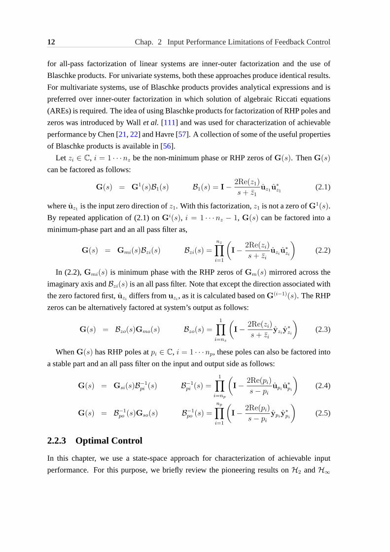
Let zi ∈ C, i = 1 · · ·nz be the non-minimum phase or RHP zeros ofG(s). ThenG(s)
can be factored as follows:
G(s) = G1(s)B1(s) B1(s) = I− 2Re(z1)
s + z1
uz1u∗z1
(2.1)
whereuz1 is the input zero direction ofz1. With this factorization,z1 is not a zero ofG1(s).
By repeated application of (2.1) on Gi(s), i = 1 · · ·nz − 1, G(s) can be factored into a
minimum-phase part and an all pass filter as,
G(s) = Gmi(s)Bzi(s) Bzi(s) =nz∏i=1
(I− 2Re(zi)
s + zi
uziu∗zi
)(2.2)
In (2.2), Gmi(s) is minimum phase with the RHP zeros ofGm(s) mirrored across the
imaginary axis andBzi(s) is an all pass filter. Note that except the direction associated with
the zero factored first,uzidiffers fromuzi
, as it is calculated based onG(i−1)(s). The RHP
zeros can be alternatively factored at system’s output as follows:
G(s) = Bzo(s)Gmo(s) Bzo(s) =1∏
i=nz
(I− 2Re(zi)
s + zi
yziy∗zi
)(2.3)
WhenG(s) has RHP poles atpi ∈ C, i = 1 · · ·np, these poles can also be factored into
a stable part and an all pass filter on the input and output side as follows:
G(s) = Gsi(s)B−1pi (s) B−1
pi (s) =1∏
i=np
(I− 2Re(pi)
s− pi
upiu∗pi
)(2.4)
G(s) = B−1po (s)Gso(s) B−1
po (s) =
np∏i=1
(I− 2Re(pi)
s− pi
ypiy∗pi
)(2.5)
2.2.3 Optimal Control
In this chapter, we use a state-space approach for characterization of achievable input
performance. For this purpose, we briefly review the pioneering results onH2 andH∞
Sec. 2.2 Preliminaries 13
K
wz
uy
A Bw B
Cz 0 D12
C D21 0
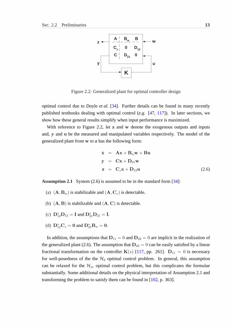
Figure 2.2:Generalized plant for optimal controller design
optimal control due to Doyleet al. [34]. Further details can be found in many recently
published textbooks dealing with optimal control (e.g. [47, 117]). In later sections, we
show how these general results simplify when input performance is maximized.
With reference to Figure2.2, let z and w denote the exogenous outputs and inputs
and,y andu be the measured and manipulated variables respectively. The model of the
generalized plant fromw to z has the following form:
x = Ax + Bww + Bu
y = Cx + D21w
z = Czx + D12u (2.6)
Assumption 2.1 System (2.6) is assumed to be in the standard form [34]:
(a) (A,Bw) is stabilizable and(A,Cz) is detectable.
(b) (A,B) is stabilizable and(A,C) is detectable.
(c) D∗12D12 = I andD∗
21D21 = I.
(d) D∗12Cz = 0 andD∗
21Bw = 0.
In addition, the assumptions thatD11 = 0 andD22 = 0 are implicit in the realization of
the generalized plant (2.6). The assumption thatD22 = 0 can be easily satisfied by a linear
fractional transformation on the controllerK(s) [117, pp. 261]. D11 = 0 is necessary
for well-posedness of the theH2 optimal control problem. In general, this assumption
can be relaxed for theH∞ optimal control problem, but this complicates the formulae
substantially. Some additional details on the physical interpretation of Assumption2.1and
transforming the problem to satisfy them can be found in [102, p. 363].

14 Chap. 2 Input Performance Limitations of Feedback Control
It follows from Assumption2.1(a)-(b) that there existX2,Y2 º 0, which solve the
following algebraic Riccati equations (AREs),
A∗X2 + X2A−X2BB∗X2 + C∗zCz = 0
AY2 + Y2A∗ −Y2C
∗CY2 + BwB∗w = 0
Let Tzw be the closed loop transfer matrix fromw to z. The unique controller
minimizing‖Tzw(s)‖2 is given as [34]:
Kopt(s) =
[A + BF2 + L2C −L2
F2 0
](2.7)
whereF2 = −B∗X2, L2 = −Y2C∗ and the optimal cost is [117],
I22 = inf
K(s)‖Tzw(s)‖2
2 = tr(B∗wX2Bw) + tr(F2Y2F
∗2) (2.8)
For the minimization of‖Tzw(s)‖∞, let X∞,Y∞ º 0 solve the following algebraic
Riccati equations,
A∗X∞ + X∞A−X∞(γ−2BwB∗w −BB∗)X∞ + C∗
zCz = 0 (2.9)
AY∞ + Y∞A∗ −Y∞(γ−2C∗zCz −C∗C)Y∞ + BwB∗
w = 0 (2.10)
where γ > 0. The existence ofX∞,Y∞ º 0 that solve the AREs (2.9)- (2.10)
is guaranteed, if Assumption2.1 holds andρ(X∞Y∞) < γ2. A suboptimal controller
achieving‖Tzw(s)‖∞ < γ is [34]:
Ksub(s) =
[A + γ−2BwB∗
wX∞ + BF∞ + Z∞L∞C −Z∞L∞F∞ 0
](2.11)
whereF∞ = −B∗X∞, L∞ = −Y∞C∗ andZ∞ = (I − γ−2ρ(X∞Y∞))−1. The optimal
cost is given as
I∞ = infK(s)
‖Tzw(s)‖∞ = ρ12 (X∞Y∞) (2.12)
2.2.4 Hankel Singular Values and Balanced Realization
It is shown later in this chapter that the achievable input performance of a system primarily
depends on the Hankel singular values of the image of the unstable part of the system. The
concept of Hankel singular values is introduced next.

Sec. 2.2 Preliminaries 15
Definition 2.4 For a rational stable systemG(s) ↔ (A,B,C,D), let XH ,YH º 0 solve
the following Lyapunov equations,
AXH + XHA∗ + BB∗ = 0 (2.13)
A∗YH + YHA + C∗C = 0 (2.14)
Then, the Hankel singular values ofG(s), σHi(G(s)) are given asσHi(G(s)) =
λ1/2i (XHYH) [42, 117].
Note that the Hankel singular values are independent of theD matrix of the state space
realization of the system. This follows as theD matrix represents the direct effect of
inputs on outputs, but the Hankel singular values measure the effect of past inputs on future
outputs [42].
The matricesXH andYH are called the controllability and observability gramians of
the system. If all the poles of the system are controllableXH Â 0. In this sense, the larger
the eigenvalues ofXH are, the more controllable are the modes of the system. Similar
conclusions can be drawn for the observability of modes based on the eigenvalues ofYH .
As σHi(G(s)) = λ1/2i (XHYH), the Hankel singular values are often referred to as the
measure of the joint controllability and observability of the modes of the system.
It is well known that the state space realization of a system is not unique. LetT be
a non-singular state transformation matrix. Then, if(A,B,C,D) is one realization of
the systemG(s), so is (T−1AT,T−1B,CT,D). One particular realization that is of
immediate interest to us is the balanced realization, as introduced next.
Definition 2.5 For a rational stable systemG(s), the state-space realizationG(s) ↔(A,B,C,D) is called a balanced realization, ifXH ,YH º 0 that solve the Lyapunov
equations (2.13)-(2.14) are diagonal and equal [42, 117].
As it turns out that for the balanced realization, the controllability and observability
gramians are equal todiag(σHi(G(s))), i.e., the matrix containing the Hankel singular
values as its diagonal elements. Any rational stable system admits a balanced realization
and an algorithm for the construction of balanced realization is available in [117]. The
balanced realization is frequently used in obtaining approximate low order models for a
system with a large number of states [42].
For later development in this chapter, we derive the balanced state-space realization of
the Blaschke productB−1po (s). For notational simplicity, we consider that the number of
unstable poles,np ≤ 2, which can be easily extended to systems withnp > 2 by induction.

16 Chap. 2 Input Performance Limitations of Feedback Control
A similar method has been used by Chen [22] earlier for finding the balanced realization of
Bzi(s).
Let B−1po (s) = B−1
p2B−1
p1(s). Using (2.4), the balanced realization ofB−1
pi(s) is given as
B−1pi
(s) ↔ (Ai,Bi,Ci,Di), where
Ai = pi Bi = −√
2Re(pi) y∗piCi =
√2Re(pi) ypi
Di = I (2.15)
Using (2.15), the balanced realization ofB−1po (s) is given asB−1
po (s) ↔ (A,B,C,D),
where
A =
[A2 B2C1
0 A1
]=
[p2 2
√Re(p1)Re(p2) y∗p2
yp1
0 p1
]
B =
[B2D1
B1
]=
[ −√
2Re(p2) y∗p2
−√
2Re(p1) y∗p1
]
C =[
C2 D2C1
]=
[ √2Re(p2) yp2
√2Re(p1) yp1
]
D = D2D1 = I (2.16)
2.3 Problem Formulation and Simplification
In this section, we formulate an optimal controller design problem that minimizes input
usage for stabilization. It is shown how the general results on optimal control can be
simplified when only input performance is considered. This simplification in turn enable
us to explicitly characterize the achievable input performance.
Consider the system shown in Figure2.3, where all exogenous inputs,e.g. load change,
measurement noise, set point change, have been collected in the blockGw(s). The closed
loop transfer matrix from disturbances to inputs is given as,
Tuw(s) = WuK(s) (I + GK(s))−1 Gw(s) (2.17)
The objective is to characterize the minimal input usage required for stabilization
expressed in terms of the norm ofTuw(s) as:
Ii = ‖WuK(s) (I + GK(s))−1 Gw(s)‖i i = 2,∞ (2.18)
Assumption 2.2 We make the following assumptions:
(a) G(s) is strictly proper.

Sec. 2.3 Problem Formulation and Simplification 17
Figure 2.3:Closed loop system for characterization of achievable input performance
(b) Wu(s) is left invertible and (if unstable) has the same unstable poles asG(s) with
the associated input pole directions.
(c) Gw(s) is right-invertible and (if unstable) has the same unstable poles asG(s) with
the associated output pole directions.
Assumption2.2(a) is made for notational simplicity and the extension to the general case
is simple (see [117, p.261] for details). The left and right invertibility ofWu(s) andGw(s)
respectively ensures that the optimal controller design problem is nonsingular.
To illustrate the necessity ofWu(s) andGw(s) having the same unstable poles asG(s)
with the associated input and output pole directions respectively, consider thatWu(s) = I
andGw(s) has a single unstable polepw such thatG−1w (pw)ypw = 0. Let {pi} ∈ Cnp be
the unstable poles ofG(s) such thatG−1(pi)ypi= 0. For internal stability, the unstable
poles ofG(s) andGK(s) are the same and
K−1G−1(pi)ypi= 0
(I + K−1G−1(pi)
)ypi
= ypi
GK(pi) (I + GK(pi))−1 ypi
= ypi
K(pi) (I + GK(pi))−1 ypi
= G−1(pi)ypi= 0 (2.19)
It follows from (2.19) that the locations of RHP zeros and output zero directions of
K(s) (I + GK(s))−1 are the same as the locations of the RHP poles and input pole
directions ofG(s). Defining the sensitivity function asS(s) = (I + G(s)K(s))−1 and
using results on Blaschke products (2.2) and (2.5),
KSGw(s) = [KS(s)]mi Bzi[KS(s)]B−1po [Gw(s)] [Gw(s)]so
= [KS(s)]mi Bpo[G(s)]B−1po [Gw(s)] [Gw(s)]so
If the controller is designed to stabilizeKS(s), the stability ofTuw(s) depends on the
stability ofBpo[G(s)]B−1po [Gw(s)]. Since the Blaschke products can be calculated for any

18 Chap. 2 Input Performance Limitations of Feedback Control
permutation of poles and zeros,Bpo[G(s)]B−1po [Gw(s)] is stable iffpw = pi andypw = ypi
for somei. Similar conclusions can be drawn whenGw(s) has more than one unstable pole
or whenWu(s) is also unstable.
With Assumption2.2, Let Wu(s) andGw(s) be factorized as
Wu(s) = B−1po [Wu(s)]Bzo [Wu(s)] [Wu(s)]sm
Gw(s) = [Gw(s)]sm B−1pi [Gw(s)]Bzi [Gw(s)]
where[Wu(s)]sm and[Gw(s)]sm are the stable minimum-phase parts ofWu(s) andGw(s)
respectively. Define
G(s) = [Gw(s)]−1sm G(s) [Wu(s)]
−1sm (2.20)
K(s) = [Wu(s)]sm K(s) [Gw(s)]sm
whereG(s) is anny × nu dimensional transfer matrix. It follows from (2.17) that
Ii = ‖B−1po [Wu(s)]Bzo [Wu(s)] K(s)(I + GK(s))−1·
B−1pi [Gw(s)]Bzi [Gw(s)] ‖i i = 2,∞ (2.21)
By simplifying (2.21),
Ii = ‖K(s)(I + G(s)K(s))−1‖i i = 2,∞ (2.22)
We point out that in (2.22), B−1po [Wu(s)] andB−1
pi [Gw(s)] can be factored out without
jeopardizing the internal stability, only when Assumptions2.2(b)-(c) are satisfied. Now,
‖Tuw(s)‖i, i = 2,∞ is minimized by designing an optimal controller forG(s), where
the following are equivalent: (a)K(s) stabilizesG(s), and (b)K(s) stabilizesG(s). In
the remaining discussion, we treatG(s) as the system without loss of generality. These
manipulations further allows us to represent the generalized plant as
˙x = Ax + Bu
y = Cx + w
z = u (2.23)
whereG(s) ↔ (A, B, C). Notice that we have transformed a controller design problem
where the closed loop system is driven by disturbances filtered through an arbitrary
disturbance model to an equivalent problem, in which the closed loop system is driven
by measurement noise only. The latter problem is much simpler to solve, as demonstrated
later in this section.

Sec. 2.3 Problem Formulation and Simplification 19
Figure 2.4:Simplifying transformations on the closed loop system
For the system (2.23), let X2, Y2 andX∞, Y∞ be the solutions of corresponding AREs
for theH2 and theH∞ optimal control (see§ 2.2.3). By comparing (2.23) with (2.6),
we notice that for the system (2.23), the corresponding AREs for theH2 andH∞ optimal
controller design are the same. It follows thatX2 = X∞ = X andY2 = Y∞ = Y. This
observation in turn implies thatF2 = F∞ = F andL2 = L∞ = L.
Let T be a state transformation matrix such thatT−1AT = diag(Ps,P), wherePs and
P contain all the stable and unstable modes respectively. Rearranging and partitioning the
states of the transformed system
˙x = T−1ATx + T−1Bu =
[Ps 00 P
]x +
[Bs
B
]u
y = CTx + w =[
Cs C]x + w (2.24)
Let X = T−1XT andY = T−1YT solve the corresponding AREs for the transformed
system (2.24). Then, to be non-negative definite,X andY must assume the form
X =
[0 00 X
]Y =
[0 00 Y
]
whereX,Y ∈ Cnp×np  0 and it suffices to solve
XP + P∗X−XBB∗X = 0 (2.25)
YP∗ + PY −YC∗CY = 0 (2.26)
Let G(s) = G1(s) + G2(s) such thatG1(s) = U(G(s)) andG2(s) ∈ RH∞, where
U(G(s)) is the unstable part ofG(s). The triplet(P,B,C) can be seen as the realization of
G1(s) and (2.25)-(2.26) as the corresponding AREs forG1(s). Then the achievable input
performance depends only on the unstable part of the system. This is further illustrated by
definingK(s) = K1(s)(I− G2K1(s))−1. With this parametrization ofK(s),
K(s)(I− GK(s))−1 = K1(s)(I− G2K1(s))−1

20 Chap. 2 Input Performance Limitations of Feedback Control
ThusK(s) exactly cancels the stable part of the system. The different transformations used
in this section and their equivalence are shown in Figure2.4.
For the transformed system (2.24), the state feedback and the output injection matrices
are given as,
F = FT =[
0 F]
=[
0 −B∗X]
(2.27)
L = T∗L =[
0 L]′
=[
0 −YC∗ ]′(2.28)
By substituting forX, Y, F andL in (2.8) and (2.12), the expressions for achievable input
performance can be simplified as,
I22 = tr(FYF∗) = tr(L∗XL) (2.29)
I∞ = ρ12 (XY) (2.30)
The equations (2.25) and (2.26) form the cornerstone for much of the remaining
development in this chapter. In general, forH∞ optimal control, the resulting AREs are
dependent onγ and thus need to be solved iteratively. In contrast, the expressions (2.25)-
(2.26) are independent ofγ and can be solved directly. Further note that when (2.25)
and (2.26) are pre- and post-multiplied byX−1 andY−1, the resulting expressions are
similar to Lyapunov equations. When all the unstable poles of the system are distinct, a
closed form solution of (2.25)-(2.26) can be derived, which is expressed in terms of the
unstable poles and the matricesB andC only.
For a system with distinct unstable poles, we can select the state transformation matrix
T such thatP is diagonal and is given asP = diag(p1, · · · , pnp), Re(pi) > 0. Let the
Hermitian matrixM ∈ Cnp×np be defined as
[mij] = 1/(pi + p∗j) (2.31)
Lemma 2.1 For a system with distinct poles, letX,Y Â 0 solve the AREs (2.25)-(2.26)
andM be given by (2.31). Then
X−1 =nu∑i=1
diag(Bi) M diag(Bi)∗ (2.32)
Y−1 =
ny∑j=1
diag(C′j)∗ M diag(C
′j) (2.33)
Proof: Pre- and post-multiplying (2.25) by X−1 gives
PX−1 + X−1P∗ = BB∗ (2.34)

Sec. 2.4 SISO systems 21
Then [63], X−1 = M ◦ (BB∗), where◦ is the Hadamard or element-wise product.
Noting thatBB∗ =∑nu
i=1 BiB∗i ,
X−1 =nu∑i=1
M ◦ (BiB∗i )
and (2.32) follows. Equation (2.33) follows from a dual argument.
2.4 SISO systems
In this section, we quantify achievable input performance of SISO systems with and without
time delay. It is assumed that all the unstable poles of the system are distinct. With this
assumption, the expressions for the achievable input performance can be expressed in terms
of the unstable poles and the matricesB andC only. The general case is considered in the
next section.
2.4.1 Rational Systems
We derive the expressions for achievable input performance for rational SISO systems next.
The usefulness of these expressions is demonstrated using a process design example. These
results also form the basis for derivation of similar expressions for SISO systems with time
delay.
Lemma 2.2 ForM defined by (2.31), letpi 6= pj for all i, j = 1 · · ·np. ThenM−1 is given
as
[M−1]ij =(p∗i + pi)(pj + p∗j)
p∗i + pj
np∏k=1k 6=i
(p∗i + pk)
(p∗i − p∗k)
np∏k=1k 6=j
(pj + p∗k)(pj − pk)
Lemma2.2 is easily verified by evaluatingMM−1 or M−1M. Note for SISO systems,
b = [bi], b = [cj].
Proposition 2.1 For a rational SISO systemg(s) with distinct poles, letU(g(s)) ↔(P,b, c) such thatP = diag(p1 · · · pnp), Re(pi) > 0. Then
I22 =
[ |qi|2bici
]M
[ |qi|2b∗i c
∗i
]T
(2.35)
I2∞ = |λ−1(diag(b∗i c
∗i ) M diag(bici) M)| (2.36)
whereM is defined by (2.31) andqi is the sum ofith column ofM−1 or q = 1Tnp
M−1.

22 Chap. 2 Input Performance Limitations of Feedback Control
Proof: (1) For (2.35), substituting forX andY in (2.29) using Lemma2.1,
I22 = fYf∗ = b∗XYXb
= 1Tnp
M−1 (diag(b)diag(c))−1 M−1(diag(b∗)diag(c∗))−1 M−1 1np (2.37)
Based on Lemma2.2,
qi = (pi + p∗i )np∏k=1k 6=i
(pi + p∗k)(pi − pk)
; i = 1 · · ·np (2.38)
andM−1 = diag(q∗)Mdiag(q). By substituting forM−1 and1Tnp
M−1, (2.37) can be
simplified as,
I22 = q (diag(b)diag(c))−1 diag(q∗) M diag(q) (diag(b∗)diag(c∗))−1 q∗
The equation (2.35) can be now obtained by simplifying the above expression using the
identityqiq∗i = |qi|2.
(2) For (2.36),
I2∞ = ρ(XY) =
∣∣λ−1(Y−1X−1)∣∣
By substituting forX−1 andY−1 using Lemma2.1
I2∞ =
∣∣λ−1(diag(c∗) M diag(c) diag(b) M diag(b)∗)∣∣
=∣∣λ−1(diag(b)∗ diag(c∗) M diag(c) diag(b) M)
∣∣=
∣∣λ−1(diag(b∗i c∗i ) M diag(bici) M)
∣∣
In the realization,U(g(s)) ↔ (P,b, c), wheng(s) has only real unstable poles only,
b∗ = b andc∗ = c. In this case, (2.36), can be further simplified as,
I2∞ = λ−1
((diag(bici)M)2 )
I∞ =∣∣λ−1(diag(bici)M)
∣∣
Remark 2.1 The expression forq in (2.38) appears to suggest that in general,I2 →∞ as
pi → pj for somei, j, which is clearly not true. Sincebici = [g(s)(s− pi)]s=pi, bici →∞,
aspi → pj, which negates the effect ofq. But when the system has an RHP zero close
to RHP poles,bici fails to increase monotonically and stabilization can be difficult. For
example, considerg(s) = (s−p)(s−p+ε)(s−p−ε)
. As ε → 0, the RHP poles approach the zero. Due
to near cancellation of the unstable pole by the zero,I2, I∞ →∞ asε → 0.
Sec. 2.4 SISO systems 23
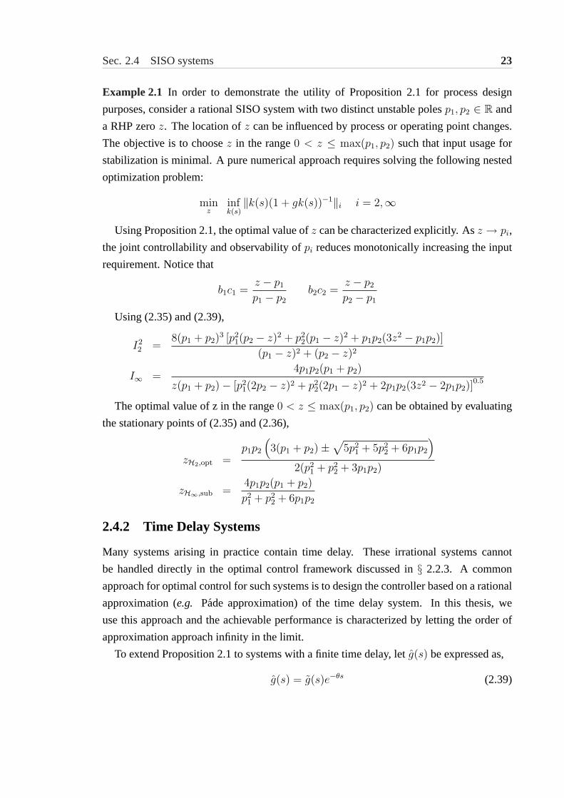
Example 2.1 In order to demonstrate the utility of Proposition2.1 for process design
purposes, consider a rational SISO system with two distinct unstable polesp1, p2 ∈ R and
a RHP zeroz. The location ofz can be influenced by process or operating point changes.
The objective is to choosez in the range0 < z ≤ max(p1, p2) such that input usage for
stabilization is minimal. A pure numerical approach requires solving the following nested
optimization problem:
minz
infk(s)
‖k(s)(1 + gk(s))−1‖i i = 2,∞
Using Proposition2.1, the optimal value ofz can be characterized explicitly. Asz → pi,
the joint controllability and observability ofpi reduces monotonically increasing the input
requirement. Notice that
b1c1 =z − p1
p1 − p2
b2c2 =z − p2
p2 − p1
Using (2.35) and (2.39),
I22 =
8(p1 + p2)3 [p2
1(p2 − z)2 + p22(p1 − z)2 + p1p2(3z
2 − p1p2)]
(p1 − z)2 + (p2 − z)2
I∞ =4p1p2(p1 + p2)
z(p1 + p2)− [p21(2p2 − z)2 + p2
2(2p1 − z)2 + 2p1p2(3z2 − 2p1p2)]0.5
The optimal value of z in the range0 < z ≤ max(p1, p2) can be obtained by evaluating
the stationary points of (2.35) and (2.36),
zH2,opt =p1p2
(3(p1 + p2)±
√5p2
1 + 5p22 + 6p1p2
)
2(p21 + p2
2 + 3p1p2)
zH∞,sub =4p1p2(p1 + p2)
p21 + p2
2 + 6p1p2
2.4.2 Time Delay Systems
Many systems arising in practice contain time delay. These irrational systems cannot
be handled directly in the optimal control framework discussed in§ 2.2.3. A common
approach for optimal control for such systems is to design the controller based on a rational
approximation (e.g. Pade approximation) of the time delay system. In this thesis, we
use this approach and the achievable performance is characterized by letting the order of
approximation approach infinity in the limit.
To extend Proposition2.1to systems with a finite time delay, letg(s) be expressed as,
g(s) = g(s)e−θs (2.39)

24 Chap. 2 Input Performance Limitations of Feedback Control
whereg is the delay-free part of the system. Ifgw(s) also contains delay, the delay can be
factored as an all-pass factor and thusg(s) remains causal (cf. (2.20)).
Lemma 2.3 ConsiderH(s) ↔ (P,B,C) such thatP = diag(p1 · · · pnp), Re(pi) > 0,
pi 6= pj. Let H1(s) ∈ RH∞ with no zeros atpi. Then
U(H1(s)H(s)) =
np∑i=1
1
s− pi
H1(pi)CiB′i (2.40)
Proof: Using dyadic expansion ofH(s),
H(s) =
np∑i=1
1
s− pi
CiB′i
Let U(H1(s)H(s)) ↔ (P, B, C). SinceH1(s) does not cancel RHP poles ofH(s),
P = P. Now, CiB′i = [H1(s)H(s)(s− pi)]s=pi
and (2.40) follows.
Note that the applicability of Lemma2.3 is not limited to the case where all modes of
H(s) are unstable, sinceU(H1(s)H(s)) = U(H1(s)U(H(s))).
Proposition 2.2 Let the SISO system expressed by (2.39) have distinct unstable poles
and U(g(s)) ↔ (P, b, c) such thatP = diag(p1 · · · pnp), Re(pi) > 0 and Γ =
diag(eθp1 · · · eθpnp ). Then
I22 =
[ |qi|2bici
]ΓMΓ∗
[ |qi|2b∗i c
∗i
]′i = 1 · · ·np (2.41)
I2∞ = |λ−1(Γ−∗diag(b∗i c
∗i )MΓ−1diag(bici)M)| (2.42)
whereM is defined by (2.31) andq = 1′np
M−1.
Proof: Let f(θs, n) be the nth order rational approximation ofe−θs (e.g. Pade
approximation). For anyn, if a RHP zero off(θs, n) cancels a RHP pole ofG(s), the
system is not stabilizable due to presence of hidden unstable modes. However, asn →∞,
the magnitude of RHP zeros off(θs, n) approaches infinity. Thus, for an FDLTI system
with poles at finite locations, such cancellation of RHP pole ofG(s) by an RHP zero of
f(θs, n) does not occur for alln ≥ N for sufficiently largeN .
(1) For (2.41), using (2.40), bici ≈ bicif(θpi, n), n ≥ N and
I22 (n) =
[ |qi|2bicif(θpi, n)
]M
[ |qi|2b∗i c
∗i f(θpi, n)
]′
=
np∑i=1
np∑j=1
|qi|2bici
|qj|2bj cj
mijf−1(θpi, n)f−1(θpj, n) (2.43)

Sec. 2.4 SISO systems 25
As limn→∞ f(θpi, s) = e−θs. Then, limn→∞ f−1(θpi, n) = eθpi and
limn→∞ f−1(θpi, n)f−1(θpj, n) = eθpieθpj . Noting that except the bilinear term
f−1(θpi, n)f−1(θpj, n), all other terms in (2.43) are independent ofn, we conclude that
limn→∞ I22 (n) exists and is given by (2.41).
(2) For (2.42), using similar arguments as before and following the proof of
Proposition2.1,
I2∞(n) =
∣∣∣λ−1(diag(f(θpi, n))−∗ diag(b∗i c∗i ) M diag(f(θpi, n))−1 diag(bici)M)
∣∣∣
The eigenvalues are roots of a polynomial equation, whose coefficients are functions
of f−1(θpi, n). As n → ∞, these coefficients and thus the roots converge. Hence,
limn→∞ I2∞(n) exists and is given by (2.42).
Similar to (2.39), for a system with real unstable poles only, (2.42) can be simplified to
I2∞ =
∣∣λ−1(Γ−1diag(bici)M)∣∣
By differentiating (2.41) with respect toθ,
dI22
dθ=
np∑i=1
np∑j=1
pipj|qi|2bici
|qj|2bj cj
mijepiθepjθ
≥ mini
p2i I
22
Thus,dI2/dθ > 0 for all θ. Similar conclusions can be drawn by differentiatingI∞ with
respect toθ. This shows that for SISO systems, the input usage cannot be decreased by
introducing additional lag in the system. Surprisingly, for MIMO systems, such an intuitive
conclusion does not hold, as is shown later.
Corollary 2.1 Under the same conditions as Proposition2.2, let gp(s) ↔ (P,Γ−1b, c) or
(P, b, cΓ−1). ThenI2(g(s)) = I2(gp(s)) andI∞(g(s)) = I∞(gp(s)).
It follows from corollary 2.1 that I2 and I∞ for a time delay system depend on its
unstable projection, which is rational.
Corollary 2.2 For a SISO system with a single real unstable polep,
I22 =
8p3e2pθ
b2c2I∞ =
2pepθ
|bc| (2.44)

26 Chap. 2 Input Performance Limitations of Feedback Control
Corollary 2.2 can be shown to be true by considering (2.41) and noting that in this
caseb, c are scalars andM = 1/2p. For delay-free systems, Havre and Skogestad [58]
earlier obtained expressions similar to (2.44). Propositions2.1 and2.2 can be seen as the
generalizations of the results of avre and Skogestad [58] to SISO systems with multiple
unstable poles and time delay.
Remark 2.2 The time-delay enters (2.41)-(2.42) assuming the formeθpi and thus does
not pose any serious limitations on input performance for systems with slow instabilities
and vice versa. It follows from Corollary 2.1 that time delay essentially reduces the
controllability (or observability) of poles and the faster the instability, the weaker the
controllability (or observability) of the pole is, as compared to the delay-free system.
2.5 MIMO systems
In this section, we generalize the results of the previous section to MIMO systems. It is
shown that the achievable input performance primarily depends on the joint controllability
and observability of unstable poles of the system. These results can be directly used for
selection of the subset of controlled and manipulated variables for stabilization.
2.5.1 Rational Systems
Similar to SISO systems, the achievable input performance is first characterized for rational
systems. These results are extended to MIMO systems with time delay later in this section.
To obtain expressions forI2 andI∞ for MIMO systems, we relateX andY solving the
AREs (2.9)-(2.10) to the Hankel singular values ofU(G(s))∗. WhenG(s) has distinct
unstable poles, the next lemma also provides an alternate expression for the Hankel singular
values ofU(G(s))∗, which can also be of independent interest.
Lemma 2.4 Let G(s) be a rational system andX,Y Â 0 solve the corresponding
AREs (2.25)-(2.26). Then,
σ2Hi(U(G(s))∗) = λi(X
−1Y−1) i = 1, · · ·np (2.45)
Further, if ˆG(s) has distinct unstable poles, letU(G(s)) ↔ (P,B,C), such thatP =
diag(p1 · · · pnp), Re(pi) > 0. ThenσHi(U(G(s))∗) is given as,
σHi(U(G(s))∗) = λ12i
[((BB∗) ◦M
)((C∗C) ◦M
)](2.46)
whereU(·) denotes the unstable part andM is defined by (2.31).

Sec. 2.5 MIMO systems 27
Proof: Pre- and post-multiplying (2.34) by T1 andT∗1 respectively, whereT1 is a state
transformation matrix,
T1PX−1T∗1 + T1X
−1P∗T∗1 = T1BB∗T∗
1
⇔ PX−1 + X−1P∗ = BB∗ (2.47)
whereP = T1PT−11 , B = T1B andX = T−∗
1 XT−11 . Similarly, by settingC = CT−1
1
andY = T1YT∗1,
P∗Y−1 + Y−1P = C∗C (2.48)
Now Y−1 andX−1 are the controllability and observability gramians of the stable system
U(G(s))∗ ↔ (−P∗, C∗, B∗) and (2.47)-(2.48) are the corresponding Lyapunov equations.
If T1 is chosen such that(−P∗, C∗, B∗) is a balanced realization, thenX−1 = Y−1 =
diag(σHi(U(G(s))∗)) [117] and
σ2Hi(U(G(s))∗) = λi(X
−1Y−1) = λi(T−∗1 X−1Y−1T∗
1) = λi(X−1Y−1)
WhenG(s) has distinct unstable poles, the alternate expression for the Hankel singular
values ofU(G(s))∗ can be obtained by substituting forX−1 and Y−1 in (2.45) using
Lemma2.1.
Proposition 2.3 For the rational MIMO systemG(s) having np unstable poles, let
(−P∗, C∗, B∗) be the balanced realization ofU(G(s))∗. Then
I22 =
np∑i=1
2|Re(Pii)|σ2
Hi(U(G(s))∗)(2.49)
I∞ = σ−1H (U(G(s))∗) (2.50)
Proof: (1) For (2.49), based on the expression forI22 (2.29),
I22 = tr(B∗XYXB) = tr(B∗XYXB) = tr(BB∗XYX)
DefineΣH = diag(σHi(U(G(s))∗)). Since(−P∗, C∗, B∗) is the balanced realization
of U(G(s))∗, using Lemma2.4and settingX = Y = Σ−1H ,
I22 = tr
[(−PΣH − ΣHP∗)Σ−3
H
]
= tr(−PΣ−2H ) + tr(−Σ−2
H P∗) =
np∑i=1
|Pii + P∗ii|
σ2Hi(U(G(s))∗)

28 Chap. 2 Input Performance Limitations of Feedback Control
where|Pii + P∗ii| = 2|Re(Pii)|.
(2) For (2.50), based on the expression forI∞ (2.30) and Lemma2.4
I∞ = λ−12 (X−1Y−1) = σ−1
H (U(G(s))∗)
The expressions (2.49)-(2.50) show thatI2 andI∞ mainly depend onσHi(U(G(s))∗),
which is a measure of joint controllability and observability of the unstable poles.
Glover [43] studied the robust stability of systems in the presence of additive
unstructured uncertainty. With the additive description of uncertainty, maximizing robust
stability is equivalent to minimizing theH∞ norm of transfer matrix from disturbances
to inputs. Thus, the results of Glover [43] are also applicable to the present case of
minimization of input energy required for stabilization. The expression forI∞ as derived
here is as an alternative proof of the similar result of Glover [43], but is generalized to the
case whereWu(s) andGw(s) can be minimum phase and share common unstable poles
with the system.
Remark 2.3 In general,H2 andH∞ norms of a transfer matrix can be arbitrarily apart.
Proposition2.3shows that when input norm is minimized,I2/I∞ is always bounded as
2σ2
H(U(G(s))∗)
σ2H(U(G(s))∗)
np∑i=1
|Re(Pii)| ≤ I22
I2∞≤ 2
np∑i=1
|Re(Pii)| (2.51)
whereP is the state matrix of the balanced realization ofU(G(s)). The closeness ofI2
andI∞ follows from the fact that the related AREs (2.25)-(2.26) for theH2 andH∞ cases
are the same. The ratioκH = σH(U(G(s))∗)/σH(U(G(s))∗) is the condition number of
U(G(s))∗ expressed in terms of Hankel singular values and can be interpreted similar to
the Euclidian condition number. A system that has a large Euclidian condition number
has strong directionality and may be difficult to control [102, p.87]. Similarly,κH can be
large due to smallσH(U(G(s))∗) indicating that the input requirement for stabilization is
large. WhenκH = 1, the upper and lower bounds onI22/I2
∞ in (2.51) are the same with
I22/I
2∞ = 2
∑np
i=1 |Re(Pii)|.
In this chapter, we assumed that the disturbances enter the closed loop system through
output channels. Proposition2.3can easily be applied to cases, where disturbances enters
through input channels by settingGw(s) = G(s) (see Figure2.5). For minimum phase
systems affected by input disturbances, the expressions for achievable input performance
are much simplified, as earlier shown by Chenet al. [26]. The results of Chenet al. [26]
are shown to be a special case of Proposition2.3by the next Corollary.

Sec. 2.5 MIMO systems 29
Figure 2.5:Disturbances entering through input channels
Corollary 2.3 With reference to Figure2.5, let G(s) be minimum phase, right invertible
and hasnp unstable poles. Then,
I22 = 2
np∑i=1
Re(pi); I∞ = 1 (2.52)
Proof: Let G(s) = GsB−1po (s) such thatGs(s) is stable. WithGw(s) = G(s) and using
(2.17),
‖Tuw(s)‖ = ‖(I + KGsB−1po (s))−1KGsB−1
po (s))‖= ‖(I + KB−1
po (s))−1K(s)‖
whereK(s) = KGs(s). Let (P, B, C, D) be the balanced realization ofB−∗po (s). Since
B−∗po (s) is all-pass and stable,σHi(B−∗po (s)) = 1 [42]. Then, using Proposition2.3, I∞ = 1
and I22 =
∑np
i=1 2|Re(Pii)|. The expression forI2 follows by noting thatPii = pi (cf.
(2.16)).
The achievable input performance for multivariate systems depends on pole locations as
well as pole directions. To illustrate this, we consider two extreme cases: (1) all the pole
directions are orthogonal and (2) are co-linear with each other.
Corollary 2.4 LetG1(s) andG2(s) be rational systems with distinct unstable poles, where
U(G1(s)) ↔ (P,B1,C1), U(G2(s)) ↔ (P,B2,C2) such thatP = diag(p1 · · · pnp),
Re(pi) > 0. Let ‖[B′1]i‖2 = ‖[B′
2]i‖2, ‖[C1]i‖2 = ‖[C2]i‖2 for all i = 1 · · ·np and
y∗pi(G1(s))ypj(G1(s)) = 1 and u∗pi(G1(s))upj(G1(s)) = 1 ∀i, jand y∗pi(G2(s))ypj(G2(s)) = 0 and u∗pi(G2(s))upj(G2(s)) = 0 ∀i 6= j
Then,I∞(G1(s)) ≥ I∞(G2(s)).
Proof: Define the diagonal matricesDI = diag(‖[B′1]i‖2) = diag(‖[B′
2]i‖2) andDO =
diag(‖[C1]i‖2) = diag(‖[C2]i‖2). Based on the alternate expression for Hankel singular

30 Chap. 2 Input Performance Limitations of Feedback Control
values (2.46) andM (2.31),
σH(U(G2(s))∗) = λ
12
[((DI [u
∗pi(G2(s))upj(G2(s))]ijDI) ◦M)
((DO[y∗pi(G2(s))ypj(G2(s))]ijDO) ◦M)]
Sinceu∗pi(G2(s))upj(G2(s)) = 0 for all i 6= j,
σH(U(G2(s))∗) = λ
12
[(D2
I ◦M)(D2O ◦M)
]
= λ12 [DIdiag(1/(pi + p∗i ))DIDOdiag(1/(pi + p∗i ))DO]
= σ (DIdiag(1/(pi + p∗i ))DO) = mini
[D−1I D−1
O ]ii(pi + p∗i )−1
Similarly, it can be shown that,σH(U(G1(s))∗) = σ (DIMDO). Using Proposition2.3,
I∞(G1) = σ(D−1
I M−1D−1O
)and using Lemma2.2,
I∞(G1) ≥ maxi
[D−1I M−1D−1
O ]ii
≥ maxi
[D−1I D−1
O ]ii(p∗i + pi)
np∏k=1k 6=i
(p∗i + pk)2
(p∗i − p∗k)2
≥ maxi
[D−1I D−1
O ]ii(p∗i + pi) = I∞(G2)
where the first inequality holds since the maximum singular value of a matrix is always
greater than or equal to the individual elements of the matrix.
In Corollary2.4, the lengths of the pole vectors are assumed equal to highlight the effect
of angles between the pole directions. In general, the optimal orientation of pole directions
for input performance depends on the unstable pole locations and the Euclidian length
of pole vectors. Intuitively, the input requirement for stabilization is minimized if pole
directions are oriented such that the fastest instability is affected most and so on.
Example 2.2 Consider the following system,
G(s) =
1 0 cos(β) sin(β)0 2 sin(β) cos(β)1 0 0 00 1 0 0
; p1, p2 ∈ R, p1 < p2
For this system,u∗p,1up,2 = sin(2β). The variation ofI∞ with β is shown in Figure2.6.
The input requirement is maximum, when the pole directions are co-linear (β = 0◦) and
and is approximately4 times larger than the case, where the pole directions are orthogonal
(β = 45◦). An explanation of this observation is as follows: When the pole directions are

Sec. 2.5 MIMO systems 31
0 50 100 150 20010
20
30
40
50
0 50 100 150 20010
20
30
40
50
Figure 2.6:Effect of pole directions onI∞
co-linear, theB matrix of the state space realization ofG(s) is singular. The inputs affect
the poles only after being filtered through the singularB matrix. Though the input itself
can vary in all directions, when filtered throughB, it is effective only in a few directions
increasing the input usage for stabilization.
2.5.2 Time Delay Systems
For extending Proposition2.2 to MIMO systems, we use a similar method as used for
univariate systems,i.e. by using a rational approximation of the time delay system and
then letting the order of approximation approach infinity. We consider systems that can be
expressed as
G(s) = G(s) ◦Θ(s); Θ(s) =[e−θijs
](2.53)
whereG is the delay-free part of the system. A system such asG(s) in (2.53) with delay
associated with individual elements of the transfer matrix, which cannot be separated at
inputs or outputs, is sometimes referred to as a multiple delay system in the literature. It is
pointed out that (2.53) does not represent the most general case and in practice is satisfied
only when theWu(s) andGw(s) are diagonal. The remaining discussion in this section is
limited to the cases whereny ≥ nu and similar expressions forny < nu can be obtained
with minor modifications.
Lemma 2.5 ConsiderH(s) ↔ (P,B,C) such thatP = diag(p1 · · · pnp), Re(pi) > 0. Let
H1(s) ∈ RH∞ with no zeros atpi. Then
U(H1(s) ◦H(s)) =
np∑i=1
1
s− pi
H1(pi) ◦ (CiB′i) (2.54)

32 Chap. 2 Input Performance Limitations of Feedback Control
The proof of Lemma2.5 is similar to the proof of Lemma2.3and is omitted. We make
the following additional assumption:
Assumption 2.3 Let U(G(s)) ↔ (P, B, C). Then the matrix(CiB′i) ◦ Θ(pi) has full
column rank for alli = 1 · · ·np.
Proposition 2.4 Consider that the MIMO system expressed by (2.53) has distinct poles
and the system satisfies Assumption2.3. Let U(G) ↔ (P, B, C) such thatP =
diag(p1 · · · pnp), Re(pi) > 0. If Gp ↔ (Ap,Bp,Cp), where
Ap = diag(p1Inu · · · pnpInu); Bp = [Inu · · · Inu ]′
Cp =[(C1B
′1) ◦Θ(p1) · · · (CnpB
′np
) ◦Θ(pnp)]
Then,I2(G) = I2(Gp), I∞(G) = I∞(Gp).
Proof: Let Θ(s) be approximated by annth order rational function as before. Asn →∞,
using Lemma2.5and the same arguments as used in the proof of Proposition2.2,
U(G(s)) =
np∑i=1
1
s− pi
(CiB′i) ◦Θ(pi) (2.55)
Due to Assumption2.3, 1s−pi
Θ(pi) ◦ (CiB′i) ↔ (piInu , Inu ,Θ(pi) ◦ (CiB
′i)). Then the
result follows by considering the aggregation of these subsystems.
It is interesting to note that whenΘ(s) is unstructured (delays cannot be separated at
inputs or outputs), stabilization of the irrational system withnp unstable poles is equivalent
to stabilizing a rational system withnp × nu unstable poles. For systems not satisfying
Assumption2.3, the triplet (Ap,Bp,Cp) is not necessarily a minimal realization. This
assumption can be relaxed for generalization purposes, but this makes the expressions
difficult and complex. A practical case, where Assumption2.3 is always violated, occurs
when the delays are associated with the sensors or actuators of the system. Systems with
delay associated with sensors are handled next and the expressions for systems with delay
associated with actuators can be obtained analogously.
Corollary 2.5 Let G(s) = diag(e−θis)G(s) andU(G(s)) ↔ (P, B, C) such thatP =
diag(p1 · · · pnp), Re(pi) > 0, pi 6= pj. Let Gp(s) ↔ (P, B,Cp), where
Cp =[
diag(e−θip1)C1 · · · diag(e−θipnp )Cnp
]
Then,I2(G(s)) = I2(Gp(s)) andI∞(G(s)) = I∞(Gp(s)).

Sec. 2.5 MIMO systems 33
The proof of Corollary2.5 follows by considering (2.55) and noting that(CiB′i) ◦
Θ(pi) = diag(e−θipi)CiB′i. It was shown earlier that for SISO systems,I2, I∞ are non-
increasing functions ofθ, but this does not hold for MIMO systems.
Example 2.3 Consider the systemG(s) = G(s) ◦Θ(s), where
G(s) =
0.2 0 2 30 0.5 1 43 2 0 05 3 0 0
; Θ(s) =
[e−α1s e−α2s
e−α2s e−α1s
]
00.02
0.040.06
0.080.1
0
0.05
0.10
0.5
1
1.5
2
2.5
x 105
Figure 2.7:Variation ofI∞ with α1 andα2
The variation ofI∞ with α1, α2 is shown in Figure2.7, which leads to the counter
intuitive conclusion that the input requirement for stabilization for MIMO systems can
decrease when the delay in some of the elements of the system increases. Whenα1 6= α2,
by virtue of Proposition2.4, the unstable projection of the irrational system has4 unstable
poles (2 poles each at0.2 and 0.5). However, whenα1 = α2 = α, G(s) can be
expressed asG(s) = G(s)eαs. Then, using Corollary2.5, the unstable projection of the
irrational system has only2 unstable poles. With slight abuse of terminology, the case of
α1 = α2 = α can be interpreted as the system having4 unstable poles and2 unstable zeros
at 0.2 and0.5. Thus, whenα1 6= α2, these RHP zeros differ from their nominal values of
0.2 and0.5 and effectively reduce the joint controllability and observability of the unstable
poles. Keepingα1 (or α2) constant and increasingα2 (or α1), these RHP zeros recede away
from the unstable poles reducing the input requirement for stabilization.

34 Chap. 2 Input Performance Limitations of Feedback Control
Corollary 2.6 Consider a MIMO systemG(s) that is expressed by (2.53) and satisfies
Assumption2.3. If G(s) has a single real unstable polep,
I22 =
8p3
∑nu
i=1 σ2i ((CB′) ◦Θ(p))
I∞ =2p
σ((CB′) ◦Θ(p))(2.56)
whereU(G(s)) ↔ (p, B, C).
Proof: Define Gp(s) ↔ (pInu , Inu , (CB′) ◦ Θ(p)). Now, similar to the proof of
Proposition2.4, it can be shown thatI2(G(s)) = I2(Gp(s)), I∞(G(s)) = I∞(Gp(s)).
SinceGp(s) has a single pole repeatednu times,M = (1/2p)[1nu · · ·1nu ]. Using (2.46),
σHi(Gp(s)∗) = (1/2p)λ
1/2i
[((CB
′) ◦Θ(p))∗((CB
′) ◦Θ(p))
]
= (1/2p)σi
[(CB
′) ◦Θ(p)
](2.57)
Now, (2.56) is obtained by substituting (2.57) in the expressions forI2 andI∞ (2.49)-(2.50).
For a system that is delay free and has a single unstable pole,M = 1/2p, BB∗ = ‖B‖22
andC∗C = ‖C‖22. Then, using the alternate expression for Hankel singular values (2.46),
I22 =
8p3
‖B‖2‖C‖2I∞ =
2p
‖B‖‖C‖ (2.58)
This expression (2.58) was earlier obtained by Havre and Skogestad [58].
Propositions2.3 and 2.4 can be seen as the generalization of the results of Havre and
Skogestad [58] to systems with multiple unstable poles and time delay.
2.6 Extended Stability
The optimal controller that minimizes input requirement for stabilization cancels the stable
poles of system (see§ 2.3) and only unstable poles are moved. Though these stable poles
do not appear in the closed loop transfer matrix from the disturbances to the inputs, they
are still present in other closed loop transfer matrices,e.g. disturbances to outputs. When
the system has lightly dampened stable poles, the variability of the output may be large.
Further, when the linear model is obtained through linearization of an nonlinear system,
the large variation of the lightly dampened modes can excite some nonlinearities. It is
beneficial tostabilizethe unstable as well as stable poles of the system that are close to
the imaginary axis by moving them further into the left half of the complex plane. In the
literature, this problem is known as theα−stability problem, where all the modes of the
Sec. 2.6 Extended Stability 35
closed loop system lie in a half plane satisfyingRe(s) < −α for the given positive scalar
α (see [28] and reference within for details). In this section, we present a simple algorithm
for theα−stability problem with minimization of input usage.
For notational simplicity, we assume thatGw(s) = Wu(s) = I. The algorithm is based
on the following observation:
Observation 2.1 Let [Tuw(s)]H2,opt and [Tuw(s)]H∞,subrepresent the closed loop system
from the disturbances to the inputs with theH2 andH∞ optimal controllers implemented
respectively. Then,
(1) The poles of[Tuw(s)]H2,opt are given as the unstable poles ofG(s) mirrored across
the imaginary axis with multiplicity2.
(2) A subset of poles of[Tuw(s)]H∞,subare given as the unstable poles ofG(s) mirrored
across the imaginary axis.
Proof: (1) When only input performance is considered, the optimal controller cancels the
stable part of the system (see§ 2.3). Thus, we can consider the system as having only
unstable poles without loss of generality. LetG(s) ↔ (P,B,C), whereRe(λi(P)) > 0.
Using the expression for optimal controller (2.7),
[Tuw(s)]H2,opt =
P BF 0LC P + BF + LC −L0 F 0
=
P + BF BF 00 A + LC −LF F 0
where the second equality is obtained by using a state transformation matrixT of the form,
T =
[I II 0
]
Pre-multiplying the ARE (2.25) by X−1 and rearranging,P+BF = −X−1P∗X. Then,
λi(P + BF) = λi(−P∗), i = 1 · · ·np. Similarly post-multiplying the ARE (2.26) by Y−1,
λi(P + LC) = λi(−P∗), i = 1 · · ·np. The result follows by noting that the eigenvalues of
−P∗ are at the mirrored locations of the eigenvalues ofP.
(2) The proof is similar to the case of[Tuw(s)]H2,opt and is omitted.
The fact that the controller minimizing input energy mirrors the unstable poles was
earlier established by Kwakernaak and Sivan [76] for the LQG and by Glover [43] for
theH∞ optimal controller design problem. Kwakernaak and Sivan [76] justified this as
a balance between the gain and decay rate of the inputs. Note that in the case ofH∞optimal control, the remaining poles of[Tuw(s)]H∞,sub
are given asλ(P + Z∞LC), where

36 Chap. 2 Input Performance Limitations of Feedback Control
asγ−2 → ρ(XY)−1, Z∞ approaches singularity (cf. (2.11)). Thus, characterization of all
the poles of[Tuw(s)]H∞,subis difficult, but it does not have any effect on the algorithm for
α−stability, as presented next.
Algorithm 2.1 Consider thatG(s) is the generalized system (2.23). Theα−stability for
this system can be achieved by following steps:
(a) Translate the imaginary axis by the transformations = s + α/2.
(b) Design an optimal controller forG(s), that minimizes the input requirement for
stabilization.
(c) Use the inverse transformations = s − α/2 on Tuw(s) to get a closed loop system
that isα−stable.
Optimal Controller Design
(a) (b) (c)
Open loop stable pole Open loop unstable pole Open loop stable pole (unaffected)
Figure 2.8:Simple method forα−stability
When the imaginary axis of thes−plane is translated tos + α/2, the stable poles of
the system that satisfyRe(s) < −α/2 also appear in the RHP of thes-plane. The optimal
controller that maximizes input performance reflects the poles in RHP ofs-plane across
the imaginary axis (see Observation2.1) across the imaginary axis. Then, by inverse
transformation to thes−plane, the poles of the closed loop system satisfyRe(s) < −α.
Using Proposition2.3, the closed loop system satisfy
‖Tuw(s− α/2)‖22 =
np∑i=1
2|Re(Pii)|σ2
Hi(U(G(s− α/2))∗)
‖Tuw(s− α/2)‖∞ = σ−1H (U(G(s− α/2))∗)
Sec. 2.7 Selection of Variables for Stabilizing Layer 37
where(P, B, C) is the balanced realization ofG(s−α/2). Similar relations can be derived
for a system with time delay using Proposition2.4; however, expressing‖Tuw(s)‖ directly
in terms of‖G(s)‖ andα is difficult. This class of norms are called shifted norms and
have been discussed by Boyd and Barratt [9, Ch. 5]. Nevertheless, Algorithm2.1provides
a simplistic way of attainingα−stability using available numerical tools forH2 andH∞optimal controller design.
2.7 Selection of Variables for Stabilizing Layer
The results presented earlier in this chapter are useful for selecting a subset of controlled
and manipulated variables for stabilizing the system with minimum input usage. Clearly,
the optimal set of variables can be selected by comparing the achievable input performance
for different alternatives. A limitation of this approach is that it suffers from the curse
of dimensionality, as the number of alternatives show an exponential growth with system
dimensions. In this section, we present an iterative algorithm for finding a suboptimal
solution in finite time.
Further, selection of variables for the stabilizing layer through minimizing input usage is
beneficial, but generally there are also other criteria. For example, the effect of disturbances
on the remaining control problem (see Figure2.1) can be amplified due to closure of the
stabilizing or inner loop making the task of performance satisfaction difficult. We show
that this issue can also be addressed in the framework of input usage minimization.
2.7.1 Choice of Norm
For a rational system with a single unstable pole driven by pure measurement noise, the
optimal subset of the controlled and manipulated variables is independent of the choice
of norm [58]. In the general case, however, the choice of norm can influence the optimal
combination of variables. For example, consider the following system,
G(s) =1
(s− 1)(s− 2)
[(0.7s− 1.2) −(2.2s + 2.4)
]
where the objective is to choose one of the inputs requiring minimum usage for
stabilization. Use ofH2 andH∞ norms suggests the selection ofu2 andu1 respectively.
The appropriate norm can be chosen based on the information available regarding the
disturbance characteristics,e.g.when the disturbances can be considered to be white noise,
use ofH2 norm is appropriate. On the other hand, when only bounds on the disturbances
are available,H∞ norm should be used [115].
38 Chap. 2 Input Performance Limitations of Feedback Control
We note that theL1 norm closely addresses the physical constraints of the system
and [117]
‖K(s)S(s)‖∞ ≤ ‖K(s)S(s)‖L1
Thus, use ofH∞ norm may be preferred overH2 norm. If for some combination of
variables,‖K(s)S(s)‖∞ > β, whereβ depends on physical constraints on the manipulated
variables, system stabilization without actuator saturation using a linear feedback controller
is not possible.
2.7.2 Reducing Computational Complexity
Consider a rational system with a single unstable pole, where the closed loop system is
driven by measurement noise. For such systems,I∞ andI2 depend on‖B‖ and‖C‖ (cf.
(2.58)) and the following conclusions can be drawn:
• The optimal set ofmy controlled andmu manipulated variables can be found by
selecting variables with largest entries in theB andC matrices.
• The optimal set ofmy controlled andmu manipulated variables is always a subset of
the optimal set of(my + 1) controlled and(mu + 1) manipulated variables.
With this monotonic relationship, the optimal set of variables for stabilization can be
selected through(ny + nu) comparisons for any × nu dimensional system. Unfortunately,
this attractive result does not hold for systems with multiple unstable poles. Specifically,
consider that the set of controlled and manipulated variables be partitioned into subsets of
equal dimensions as,y = [y1 y2 y3] andu = [u1 u2 u3]. Among these subsets, let the
input requirement be minimized by choosingy1,u1. In general, there is no guarantee that
the achievable input performance for the subset[y1, y2], [u1 u2] is better than the subset
[y2, y3], [u2 u3]. This point is further illustrated using the following system:
G(s) =1
(s− 0.5)(s− 1.7)
[(−1.7s + 0.75) (−s + 1.1) −0.3(s + 0.1)
]
For this system,u3 is the optimal choice formu = 1 andu1, u2 is the optimal choice for
mu = 2, when either ofH2 orH∞ norms are minimized. Due to the lack of a monotonic
relationship,Cnymy × Cnu
mucomparisons are required for optimally selectingmy controlled
andmu variables for any×nu dimensional system. Solving the variable selection problem
through comparison of all alternatives is computationally intractable, as the number of
alternatives grow exponentially with the system dimensions. To this end, Havre [56] has

Sec. 2.7 Selection of Variables for Stabilizing Layer 39
suggested using the following step-wise approach to obtain a suboptimal solution in finite
time, where the unstable poles are stabilized one at a time:
Algorithm 2.2 For rational systems withWu(s) = Gw(s) = I,
(a) Scale the system variables and obtain a state space realization of the scaled system,
whereU(G(s)) ↔ (P,B,C) such thatP = diag(p1 · · · pnp), Re(pi) > 0.
(b) To stabilize the first real or pair of complex unstable pole (preferably the fastest
unstable pole), choose the controlled and manipulated variables with largest entries
in the corresponding rows and columns of theB andC matrices respectively. Design
a controller to stabilize the chosen unstable pole and close the loop.
(c) Similar to the previous steps, obtain a state space realization for the remaining
control problem and stabilize the second unstable pole. Repeat the procedure until
all unstable poles are stabilized.
This simple method avoids the problem of computational complexity, as in the worst
case, maximum of∑np
i=0(ny + nu − 2i) comparisons are required; however, it suffers from
the following limitations:
• Algorithm 2.2 yields a decentralized controller designed sequentially and thus the
input usage for stabilization is large as compared to a full block multivariate
controller.
• In the worst case, this method requires thatnr + nc controlled and manipulated
variables be used for a system withnr real andnc pairs of complex unstable poles.
• The algorithm does not handle time delay systems or the case whereWu(s) 6= I or
Gw(s) 6= I.
We next present an iterative method that does not suffer from the limitations of
Algorithm 2.2. The central idea is to choose one controlled or manipulated variable
at a time. The algorithm provides a reasonable suboptimal solution for the variable
selection problem in finite time, where the computational time increases linearly with
system dimensions and quadratically with the number of variables to be selected. The
case of system stabilization using decentralized controller is handled in the next chapter.
Algorithm 2.3 Prior to variable selection, scale the system variables.

40 Chap. 2 Input Performance Limitations of Feedback Control
(a) Select the optimal set consisting of1 controlled and1 manipulated variable that
minimizes input requirement for stabilization by enumerating all possibleny × nu
alternatives.
(b) Keeping the set of chosen manipulated variables the same, select an additional
controlled variable that minimizes input requirement for stabilization.
(c) Keeping the set of chosen controlled variables the same, select an additional
manipulated variable that minimizes input requirement for stabilization.
(d) Repeat steps (b) and (c) untilmy controlled andmu manipulated variables are
selected. Ifmy 6= mu, skip step (b) or (c) once the required number of variables
are selected.
Algorithm 2.3 can be easily used to handle time delay systems and the cases where
Wu(s) 6= I or Gw(s) 6= I. Note that whenWu(s) and Gw(s) are not diagonal, the
algorithm requires inversion of different sub-matrices ofWu(s) andGw(s) during every
iteration. For selecting the set ofmy controlled andmu manipulated variables for a
ny × nu dimensional system, the Algorithm2.3 requiresnynu +∑ny−my+1
i=1 (ny − i) +∑nu−mu+1j=1 (nu − j) number of comparisons. This expression can be simplified as,
nynu + (ny − 0.5my)(my − 1) + (nu − 0.5mu)(mu − 1)
Essentially, starting from the optimal set of1 controlled and1 manipulated variable,
at every step, Algorithm2.3 adds one locally optimal controlled or manipulated variable.
A similar algorithm can be constructed that starts with all variables and eliminates one
controlled or manipulated variable at every step. This alternative algorithm is particularly
useful, whenmy > ny/2 andmu > nu/2.
Example 2.4 We consider the base case of the Tennessee Eastman benchmark
problem [33]. A linearized model of this process is obtained by numerical differentiation
of the nonlinear model. The model is scaled prior to variable selection using the approach
of Havre [56, Ch.6]. Based on the recommendation of Havre [56, Ch.6], we use only a
subset of controlled variables and avoid using feed streams for stabilization. The resulting
system has11 controlled and8 manipulated variables and unstable poles at3.07 ± j5.08,
0.02± j0.16, 0.007 and0.
In Table 2.1, we show the results obtained by applying Algorithm2.3 for H∞ norm
minimization, which are compared against the optimal solution obtained by enumeration.
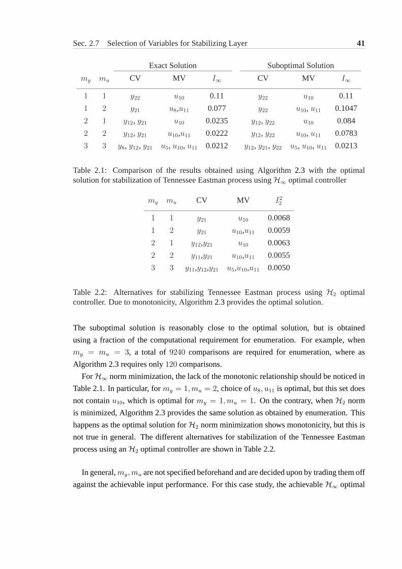
Sec. 2.7 Selection of Variables for Stabilizing Layer 41
Exact Solution Suboptimal Solution
my mu CV MV I∞ CV MV I∞
1 1 y22 u10 0.11 y22 u10 0.11
1 2 y21 u8,u11 0.077 y22 u10, u11 0.1047
2 1 y12, y21 u10 0.0235 y12, y22 u10 0.084
2 2 y12, y21 u10,u11 0.0222 y12, y22 u10, u11 0.0783
3 3 y8, y12, y21 u5, u10, u11 0.0212 y12, y21, y22 u5, u10, u11 0.0213
Table 2.1: Comparison of the results obtained using Algorithm2.3 with the optimalsolution for stabilization of Tennessee Eastman process usingH∞ optimal controller
my mu CV MV I22
1 1 y21 u10 0.0068
1 2 y21 u10,u11 0.0059
2 1 y12,y21 u10 0.0063
2 2 y11,y21 u10,u11 0.0055
3 3 y11,y12,y21 u5,u10,u11 0.0050
Table 2.2: Alternatives for stabilizing Tennessee Eastman process usingH2 optimalcontroller. Due to monotonicity, Algorithm2.3provides the optimal solution.
The suboptimal solution is reasonably close to the optimal solution, but is obtained
using a fraction of the computational requirement for enumeration. For example, when
my = mu = 3, a total of 9240 comparisons are required for enumeration, where as
Algorithm 2.3requires only120 comparisons.
ForH∞ norm minimization, the lack of the monotonic relationship should be noticed in
Table2.1. In particular, formy = 1,mu = 2, choice ofu8, u11 is optimal, but this set does
not containu10, which is optimal formy = 1,mu = 1. On the contrary, whenH2 norm
is minimized, Algorithm2.3provides the same solution as obtained by enumeration. This
happens as the optimal solution forH2 norm minimization shows monotonicity, but this is
not true in general. The different alternatives for stabilization of the Tennessee Eastman
process using anH2 optimal controller are shown in Table2.2.
In general,my,mu are not specified beforehand and are decided upon by trading them off
against the achievable input performance. For this case study, the achievableH∞ optimal

42 Chap. 2 Input Performance Limitations of Feedback Control
input performance using all controlled and manipulated variables is0.0194. Then, based
on the optimal solution obtained by enumeration, use of2 controlled and1 manipulated
variables is sufficient. In comparison, a disadvantage of Algorithm2.3 is that is suggests
use of3 controlled and3 manipulated variables and finding an improved algorithm remains
an open area of research.
2.7.3 Other Criteria
In the previous section, the selection of variables for the stabilizing layer through
minimizing input usage was demonstrated. Though beneficial, this approach can be
insufficient for practical controller design problems as generally there are also other criteria.
One such important criterion is the amplification of effect of disturbances on the remaining
control problem (see Figure2.1) due to closure of the stabilizing loop, which can make the
task of performance satisfaction difficult. We show that this issue can also be addressed in
the framework of input usage minimization.
Consider the set of controlled and manipulated variables be conformably partitioned as
y1(s) = G11(s)u1(s) + G12(s)u2(s) + Gw1(s)w(s)
y2(s) = G21(s)u1(s) + G22(s)u2(s) + Gw2(s)w(s)
where the subsety2,u2 is used for stabilization. When the stabilizing loop is closed, the
effect of the disturbance on the controlled variables of open loop system is given as [56],
y1(s) =(Gw1(s)−G12K(s)(I + G22K(s))−1Gw2(s)
)w(s)
= Gw1(s)(I−G−1
w1G12K(s)(I + G22K(s))−1Gw2(s))w(s)
Then, the stabilizing layer amplifies the effect of disturbances on the remaining control
problem, if
‖I−G−1w1(s)G12K(s)(I + G22K(s))−1Gw2(s)‖∞ > 1
During the selection of controlled and manipulated variables, it is beneficial to take this
effect of disturbance amplification into account. The stabilizing controller can be designed
such that the input usage for stabilization is traded off against the disturbance amplification
effect. For this purpose, we note that
‖I−G−1w1(s)G12K(s)(I + G22K(s))−1Gw2(s)‖∞
≤ 1 + ‖G−1w1(s)G12K(s)(I + G22K(s))−1Gw2(s)‖∞

Sec. 2.8 Chapter Summary 43
Thus, it suffices to minimizeσ(G−1w1(s)G12K(s)(I + G22K(s))−1Gw2(s)) at the
desired frequencies. In general, we can minimize‖Ww(s)G−1w1(s)G12K(s)(I +
G22K(s))−1Gw2(s)‖∞, whereWw(s) is a frequency dependent weight. This requirement
combined with minimization of input usage for stabilization results in a multi-objective
optimization problem and a popular approach is to instead solve the following optimization
problem
minK(s)
∥∥∥∥[
Wu(s)Ww(s)G−1
w1(s)G12
]K(s)(I + G22K(s))−1Gw2(s)
∥∥∥∥∞
(2.59)
This problem is the same as the general input usage minimization problem considered
earlier in this chapter, except the special choice of frequency dependent weights. Thus, the
controlled and manipulated variables can be selected as discussed in the previous section
with minor modification. ForH2 norm minimization, similar expression as (2.59) can be
used.
2.8 Chapter Summary
In this chapter, we used a state space framework to obtain analytic expressions for
achievable input performance for SISO and MIMO systems with and without time delay.
Regarding the factors affecting achievable input performance, the following general
conclusions are drawn:
1. The input performance primarily depends on the joint controllability and
observability of unstable poles.
2. In the H∞-control framework, there are no limitations on achievable input
performance for minimum phase systems, when the closed loop system is driven by
input disturbances. In theH2-control framework, the achievable input performance
for this class of systems is limited only by the location and number of unstable poles.
3. Time delay poses no serious limitation on the achievable input performance for a
system with slow instabilities andvice versa.
4. The input performance of a MIMO system, where the delays cannot be separated at
the inputs or outputs, can be much worse as compared to a system with delays that
can be factored at the inputs or outputs.

44 Chap. 2 Input Performance Limitations of Feedback Control
5. In contrast to SISO systems, the input requirement for stabilization may decrease
for MIMO systems with an increase in time delay in some elements of the transfer
matrix relating controlled and manipulated variables.
Based on the observation that the optimal controller mirrors the unstable poles across
the imaginary axis, a simple method is proposed to handle theα−stability problem. In
the context of process control, this method is useful for controller design using available
numerical tools for systems with a subset of poles on or near the imaginary axis frequently
arising due to holdup of utilities and raw materials.
It is demonstrated that except for systems with a single unstable pole, the optimal subset
of controlled and manipulated variables that minimizes input requirement for stabilization
depends on the choice of norm. In the general case, the choice of norm depends on the
available information regarding disturbance characteristics, but use ofH∞ norm can be
preferred to address the actuator saturation issue. We also presented some insights to reduce
the computational complexity of the variable selection problem and handle criteria other
than input performance maximization in a unified framework.
2.9 Further Reading on Performance Limitations
The area of fundamental limitations of feedback control can be dated back to Bode [8].
In his seminal work, Bode showed that for stable systems with more than one pole-zero
excess, the integral of logarithmic magnitude of the sensitivity function over all frequencies
is always zero. With a finite bandwidth limitation, this result implies the unavoidable trade-
off between different performance objectives. Bode’s result has been extended to open loop
unstable systems by Freudenberg and Looze [38]. The same authors have also developed
a Poisson-type integral to quantify the limitations imposed by the unstable zeros on the
sensitivity integral. The classical Bode sensitivity and Poisson-type integrals have been
extended to multivariate systems by Chen [21]. The importance of the Bode sensitivity
integral for some real-life controller design problems is discussed by Stein [104].
Note that the Bode sensitivity or Poisson integrals always hold, irrespective of the
optimal controller design criteria. A similar set of constraints, known as analyticity
or interpolation constraints, were introduced by Zames [115]. The interpolation
constraints show that for a system with unstable poles and zeros, peaks in sensitivity and
complementary sensitivity functions are inevitable [102, 115]. Havre and Skogestad [57]
have used these interpolation constraints to quantify limitations imposed by RHP poles and
zeros on the lower bounds on several important closed loop transfer matrices. Chen [22]

Sec. 2.9 Further Reading on Performance Limitations 45
has presented improved achievable bounds on the sensitivity and complementary sensitivity
functions through the use of these constraints combined with Nevanlinna-Pick interpolation
theory [6].
Over the years, a number of results have been obtained for a related class of problems,
where the achievable performance is quantified assuming a particular performance
criterion. One of the most studied problems is the singular or cheap control problem.
For discrete time systems, Peng and Kinnaert [89] have provided an explicit solution and
the achievable performance is characterized by Qiu and Davison [92]. Recently, Yuz and
Goodwin [114] presented an approximate solution to the decentralized minimum variance
control, which is also studied later in this thesis. The presented list of references on
performance limitations is far from complete. The reader is encouraged to refer to the
books [9, 97, 102] and the recently published special issue on performance limitations by
IEEE Transactions on Automatic Control [27].


Chapter 3
µ-Interaction Measure for UnstableSystems
The requirement that the block diagonal part of the system should have the same
unstable poles as the system limits the practical applicability of conventionalµ-interaction
measure (µ-IM) [ 49] to stable systems. This limitation can be overcome by designing the
decentralized controller based on a block diagonal approximation that is different from
the block diagonal elements, but has the same number of unstable poles as the system. By
expressing theµ-IM in terms of the transfer matrix between the disturbances and inputs, we
show that the block diagonal approximation can be sub-optimally selected by minimizing
the scaledL∞ distance between the system and the approximation. We present a numerical
method for choosing the block diagonal approximation and a simple method for designing
the decentralized controller based on the approximation.1
3.1 Introduction
The last chapter presented results on system stabilization using minimal control action. In
this chapter, we consider the system stabilization using a decentralized controller. Over the
years, three different approaches have evolved for decentralized controller design:
a) Simultaneous design using parametric search methods: The decentralized controller
is chosen to have a fixed structure (e.g. PID controller) with unknown parameters.
1A part of this work was performed while the author was visiting Professor Sigurd Skogestad, NorwegianInstitute of Science and Technology, Trondheim, Norway during March-May 2003.
The central idea of this chapter was presented at the American Control Conference, Boston, MA, 2004 [74].
47

48 Chap. 3 µ-Interaction Measure for Unstable Systems
The optimal value of these parameters is found by minimizing the appropriate norm
of the closed loop system using direct or indirect search based methods. Though
useful, this approach results in optimization problems that are not usually convex
and can be highly complicated even for simple systems [7].
b) Sequential design: The controllers are designed sequentially using a lexicographical
ordering of the individual controllers. The lowest level controller is designed first and
the loop is closed. The next controller is designed based on the partially closed loop
system. The resulting performance strongly depends on the ordering of the loops and
often a trial and error approach is required to obtain acceptable performance [67, 84].
c) Independent design: The individual controllers are designed independently of each
other based on a block diagonal approximation that is usually taken as the block
diagonal elements of the system. Then, the decentralized controller design problem
reduces to design of a number of small dimensional full multivariable controllers.
When the interactions are small, such a controller also stabilizes the closed loop
system with minimal loss of performance in comparison to the design basis [66, 101].
This approach always results in suboptimal performance because the tuning of other
controllers is neglected.
In this work, we focus on the independent design approach. Although sub-optimal,
the controller design is much simpler as compared to other techniques. Furthermore, this
approach easily handles the cases in which only the bounds on (possibly time-varying)
off-diagonal elements of the system are available [98].
Grosdidier and Morari [49] proposed the use ofµ interaction measure (µ-IM) to assess
the feasibility of system stabilization through independent designs of individual loops.
This approach yields sufficient conditions to ensure that the decentralized controller that
stabilizes the block diagonal part of the system also stabilizes the system itself. The
problem of decentralized controller synthesis through independent designs has also been
studied by Limbeer [78] and Ohtaet al. [88], who used the concepts of generalized
block diagonal dominance and quasi block diagonal dominance respectively. The use of
µ−IM is less conservative than these approaches because the controller structure is taken
into account. A connection between these methods based on dominance andµ−IM is
established in the next chapter.
The conventionalµ-IM requires that the system and its block diagonal part have the same
right half plane (RHP) poles. Grosdidier and Morari [49] pointed out that this condition is
not satisfied by most of the systems encountered in practice, limiting the applicability of

Sec. 3.1 Introduction 49
µ-IM to open loop stable systems. Samyudiaet al. [96] have criticized theµ-IM for this
limitation and have instead proposed a method based onν-gap metric [110]. In this chapter,
we present a modifiedµ-IM that easily handles unstable systems. The decentralized
controller is designed based on a block diagonal approximation that is different from the
block diagonal elements, but has the same number of unstable poles as the system.
Clearly, the number of block diagonal systems with the required number of unstable
poles is infinite and the success of the modifiedµ-IM approach strongly depends on the
choice of an appropriate approximation. We express theµ-IM in terms of the closed
loop transfer matrix between disturbances and system input (or controller output). This
alternate representation shows that the block diagonal approximation can be reasonably
selected by minimizing the scaledL∞ distance between the system and the approximation.
The problem of finding a structured approximation of a full multivariate system has
earlier been considered by Li and Zhou [77], but no numerical methods for solving the
approximation problem are provided. In this chapter, we present a numerical approach,
where the approximation problem is first solved at a set of chosen frequencies followed by
a parametric identification method.
Similar to the conventionalµ-IM method, the stabilizing decentralized controller can
be synthesized using a loop shaping approach based on the block diagonal approximation.
An advantage of alternate representation ofµ-IM used here is that controller design can
be much simplified using the results of last chapter. Although the focus of this chapter
is on finding stabilizing decentralized controllers, we show that the stabilizing controller
inherently minimizes an upper bound on the input requirement for stabilization. The results
presented here can also be extended to handle (robust) performance issues directly using
the results of Skogestad and Morari [101].
The organization of this chapter is as follows: some useful results from robust control
theory and optimization are presented in§ 3.2; the available results ofµ-IM are reviewed
and its limitation is pointed out in§ 3.3; the alternate representation ofµ-IM is presented
and upper bounds on closed loop performance are derived in§ 3.4; in § 3.5we consider the
problem of selecting the optimal block diagonal approximation; the simplified controller
design is presented in§ 3.6; in § 3.7, a numerical example is presented to demonstrate the
utility of proposed approach followed by chapter summary in§ 3.8.

50 Chap. 3 µ-Interaction Measure for Unstable Systems
3.2 Preliminaries
In this section, we review the useful concepts of structured singular value, model order
reduction and optimization using linear matrix inequalities. These results are used
extensively during the remaining development in this chapter.
3.2.1 Structured Singular Value
Most of the problems encountered in robust control theory can be reduced to guaranteeing
that for some characteristic transfer matrixM(s), I −M(jω)∆(jω) remains nonsingular
for all ω for all allowable values of∆(jω) ∈ Cq×p. A practical and mathematically
convenient way of representing the set of allowable∆(s) is as a norm bounded set,
e.g., σ(∆(jω)) ≤ 1 for all ω. With this representation, the smallest norm of the
destabilizing perturbation∆(jω) is given as1/σ(M(jω)). Then, it follows thatdet(I −M(jω)∆(jω)) 6= 0 for all allowable perturbations, iff‖M(s)‖∞ < 1.
In the above discussion, allowable perturbations include all matrices∆(jω) with
σ(∆(jω)) ≤ 1 for all ω. In practice, many problems arise, where∆(s) has a structure,
i.e. some entries of∆(s) are identically zero. Then, the condition‖M(s)‖∞ < 1 is
only sufficient (and highly restrictive) for ensuring thatdet(I − M(jω)∆(jω)) 6= 0 for
all allowable perturbations. This motivates the use of the structured singular value, which
explicitly accounts for the structure of the perturbations.
Definition 3.1 Let the set∆ ∈ Cp×q be defined as
∆ = {diag(∆i) : ∆i ∈ Cpi×qi , σ(∆) ≤ 1}
The structured singular value ofA ∈ Cq×p is given as [35],
µ∆(A) =1
min{σ(∆) : ∆ ∈ ∆, det(I−A∆) = 0}
unless no∆ ∈ ∆ makes(I−A∆) singular, in which caseµ∆(A) = 0.
The µ∆(A) represents2−norm of the smallest structured perturbation that makes
I −A∆ singular, where the subscript∆ is used to explicitly denote the structure. Braatz
et al.[14, 15] and Fu [39] have shown that in the general case, the determination of the exact
value or an approximate bound onµ is not computationally tractable; however this is not a
serious limitation as a tight upper bound onµ for complex structured perturbations can be
readily computed [35]. For notational simplicity, consider the perturbation set consisting

Sec. 3.2 Preliminaries 51
of square matrices and letD be set of matrices that commute with all elements of∆ or
D∆ = ∆D for all ∆ ∈ ∆,D ∈ D. Then,
µ∆(A) ≤ infD∈D
σ(DAD−1) (3.1)
In this thesis, we denote the upper bound given by (3.1) asµ∆(.). The upper bound given
by (3.1) is tight for complex perturbations and the equality holds, if the number of blocks
in ∆ is less than4. When∆ has4 or more blocks with no block being a repeated scalar,
the ratio ofµ∆(.) andµ∆(.) for the worst known example is0.85 and is close to1 for most
cases [117]. A collection of many useful properties of the structured singular value can
be found in [102, 117]. One particularly useful property of the structured singular value,
which is used later in this chapter is:
µ∆
([0 AB 0
])=
√σ(A)σ(B) (3.2)
where∆ = diag(∆1,∆2) and∆1,∆2 are full complex matrices [100].
3.2.2 Optimal Hankel Norm Approximation
For practical controller design and system identification, use of low order controllers or
models is preferred because of online implementation issues. Imposing an order constraint
directly on the controller design or identification algorithms usually makes the problem
non-convex and difficult to solve. To avoid this difficulty, we can first solve the unrestricted
problem (wrt the controller or model order) and then reduce the order of the solution using
efficient techniques. In this subsection, we discuss such an order reduction technique,i.e.,
Hankel norm approximation approach.
Let G(s) be a stable, square and rational transfer matrix having ordern. The objective
is to find a reduced order stable transfer matrixGk(s) having orderk such that
Gk(s) = arg minGk(s)
‖G(s)− Gk(s)‖H
where‖.‖H denotes the Hankel norm. This problem has been studied by many researchers
and a complete solution is given by Glover [42], who showed that
minGk(s)∈RH∞
‖G(s)− Gk(s)‖H = minGk(s),F∗(−s)∈RH∞
‖G(s)− Gk(s)− F(s)‖∞(3.3)
= σH,k+1(G(s)) (3.4)
whereσH,k+1(.) denotes the(k + 1)th Hankel singular value. A complete characterization
of all solutions that achieve the lowest approximation error (3.4) is available in the

52 Chap. 3 µ-Interaction Measure for Unstable Systems
original paper by Glover [42] and many standard optimal control textbooks. Note that
the requirement thatG(s) be square is not restrictive and is easily satisfied by padding
extra zero columns or rows on the non-squareG(s). When the order of the approximation
k is zero,Gk(s) is a constant matrix and thus (3.3) is equivalent to finding an anti-stable
approximation of a stable system. In this case, the Hankel norm approximation problem is
alternatively known as the Nehari extension problem [37].
For the block diagonal approximation problem discussed later in the chapter, we require
thatG(s) with np unstable poles be approximated byGk(s) with k unstable poles such that
‖G(s)− Gk(s)‖∞ is minimized. Next, we show that this problem can also be solved as a
Hankel norm approximation problem.
Let G(s) = G1(s) + G2(s) such thatG∗1(−s),G2(s) ∈ RH∞. Without loss of
generality, we can parameterizeGk(s) asGk(s) = Gk1(s) + G2(s), which provides
‖G(s)− Gk(s)‖∞ = ‖G1(s)− Gk1(s)‖∞ = ‖G∗
1(−s)− (Gk1(s))
∗‖∞The optimal value for(Gk
1(s))∗ ∈ RH∞ is found by solving (cf. (3.3)),
min(Gk
1(s))∗,F∗(−s)∈RH∞‖G∗
1(−s)− (Gk1(s))
∗ − F(s)‖∞
Then, the optimal value ofGk(s) is given asGk(s) = Gk1(s) + F∗(−s) + G2(s). Since
F∗(−s) andG2(s) are stable,Gk(s) is theL∞ optimal reduced order approximation of
G(s) with k unstable poles.
3.2.3 Linear Matrix Inequalities
Many control theoretic problems require solving an optimization problem that does not
admit an analytic solution. Solving these problems numerically strongly depends on
whether the optimization problem is convex and if not, how closely it can be approximated
by an equivalent convex problem. Linear matrix inequalities (LMIs) represent a class of
such convex constraints and are represented as follows,
F(x) = F0 +n∑
i=1
xiFi  0 (3.5)
wherex ∈ Rn represents the decision variable andFi ∈ Rn×n are symmetric matrices. In
(3.5), is the partial ordering symbol andF(x)  0 implies thatF(x) is positive definite.
The past decade has seen a rapid growth in the use of LMIs for solving control problems
because many non-linear optimization problems can be represented as LMIs that are affine
in the decision variables.

Sec. 3.3 µ-Interaction Measure 53
In this chapter, we use LMIs as the primary computational tool for solving relevant
optimization problems. To fully appreciate the importance of LMIs, consider the problem
of calculatingµ∆(.). Due to the presence of the inverse term in (3.1), the optimization
problem is difficult to solve in its present form; however, it can be transformed into an
equivalent convex optimization problem. There existsD ∈ D such thatµ∆(A) < γ iff
(DAD−1)∗(DAD−1) ≺ γ2I for some D ∈ D⇔ A∗D∗DA ≺ γ2D∗D for some D ∈ D
⇔ A∗PA ≺ γ2P for some P = D∗D,P Â 0,P ∈ D (3.6)
For a givenγ, (3.6) is affine in the decision variableP. Thus the minimal value ofγ
can be found using a bisection search method andµ∆(A) = inf γ such that (3.6) holds.
The class of problems having a form similar to (3.6) are known as generalized eigenvalue
problems. A collection of many other control problems that can be reduced to the LMI
form is available in [10].
Naturally, not every optimization problem can be reduced to LMIs. A more general class
of matrix inequality problems is that which involves the product of two decision variables.
These inequalities are known as bilinear matrix inequalities (BMIs) and have the following
general form,
F(x,y) = F0 +n∑
i=1
xiFi +n∑
j=1
yjGi +n∑
i=1
n∑j=1
xiyjHij  0 (3.7)
whereFi,Gj,Hij  0 for all i, j andy ∈ Rn. These BMIs are much more difficult to
solve than LMIs and are known to be computationally intractable [108]. When one of the
decision variables in (3.7) is fixed, the relation becomes an LMI. Then, the BMI (3.7) can
be sub-optimally solved by iteratively by fixing one of thex andy at a time. This simplistic
often provides satisfactory solution to the BMI. A survey of other techniques for solving
BMIs can be found in [108] and its references.
3.3 µ-Interaction Measure
In this section, we briefly review the available results onµ-IM [ 49], point to its limitation
and suggest a modification to overcome the same. Throughout this chapter, we assume
that the system does not contain any decentralized fixed modes [112]. The absence of
decentralized fixed modes is both necessary and sufficient for existence of a decentralized
stabilizing controller but only necessary, when individual loops of the decentralized
controller are designed independently of each other.

54 Chap. 3 µ-Interaction Measure for Unstable Systems
- Kbd Gbd
d
yu
G
Figure 3.1:Closed loop system
With reference to Figure3.1, let the systemG(s) be partitioned asG(s) = Gbd(s) +
GI(s) such that
• Gbd(s) contains the block-diagonal elements ofG(s) and
• Gbd(s) andG(s) have the same number of RHP poles.
Define the transfer matricesE(s) andTbd(s) as,
Tbd(s) = GbdKbd(s) (I + GbdKbd(s))−1 (3.8)
E(s) = (G(s)−Gbd(s))G−1bd (s) (3.9)
where Kbd(s) is the block diagonal controller. Tbd(s) can be interpreted as the
complementary sensitivity function ifGI(s) were zero, andE(s) as the multiplicative
uncertainty inGbd(s). Let Kbd(s) be designed such thatTbd(s) is stable. The central
question remains: DoesKbd(s) also stabilizeG(s)? This issue has been addressed by
Grosdidier and Morari [49], who proposed the use ofµ-IM for this purpose.
Lemma 3.1 Assume thatG(s) andGbd(s) have same number of RHP poles andTbd(s)
is stable. ThenT(s) = GKbd(s) (I + GKbd(s))−1 is stable iff the following conditions
hold [49]
det(I + ETbd(s)) 6= 0 (3.10)
N(0, det(I + ETbd(s))) = 0 (3.11)
whereN(α, .) denotes the winding number [110] or the number of clockwise encirclements
of the point(α, 0) by the image of NyquistD contour under (.).
Proof: The return difference transfer function forT(s) can be written as,
(I + GKbd(s)) = (I + GbdKbd(s) + GIKbd(s))
=(I + GIKbd(s)(I + GbdKbd(s))
−1)(I + GbdKbd(s))
= (I + ETbd(s)) (I + GbdKbd(s)) (3.12)

Sec. 3.3 µ-Interaction Measure 55
Since for rational systemsg1(s), g2(s), N(α, g1g2(s)) = N(α, g1(s))+N(α, g2(s)) (see
e.g.[110]), using the alternate expression for the return difference transfer function (3.12),
N(0, det(I + GKbd(s))) = N (0, det(I + ETbd(s)))
+ N(0, det(I + GbdKbd(s))) (3.13)
SinceG(s) hasnp unstable poles, it follows from the multivariate Nyquist stability
criterion [102] thatT(s) is stable iff
det(I + G(s)Kbd(s)) 6= 0
N(0, det(I + G(s)Kbd(s))) = −np
Further, sinceTbd(s) is stable by assumption,
det(I + Gbd(s)Kbd(s)) 6= 0
N(0, det(I + Gbd(s)Kbd(s))) = −np
The necessity and sufficiency of (3.10)-(3.11) follows using above expressions and
(3.13).
Lemma3.1was originally proven by Grosdidier and Morari [49], except the requirement
that (3.10) must hold. This is a minor technical requirement to ensure that the image of
det(I+TbdE(s)) does not pass through the origin of the complex plane. Lemma3.1forms
the basis for a more important result, as presented next.
Theorem 3.1 Let G(s) and Gbd(s) have same number of unstable poles. IfKbd(s)
stabilizesGbd(s), thenKbd(s) also stabilizesG(s), if
σ (Tbd(jω)) < µ−1∆ (E(jω)) ∀ω ∈ R (3.14)
where∆ has the same block structure asGbd(s) andTbd(s), E(s) are defined by (3.8) and
(3.9) respectively.
Proof: The sufficiency of (3.14) for closed loop stability is proven by contradiction. Let
N(0, det(I + ETbd(s))) > 0 and let the image ofdet(I + ETbd(s)) intersect the negative
real axis of complex plane at the frequencyωo. Then there exists aβ, |β| < 1 such that
det(I + βETbd(jωo)) = 0
Similarly, let there exists a frequencyω1 such that
det(I + ETbd(jω1)) = 0

56 Chap. 3 µ-Interaction Measure for Unstable Systems
Combining these two conditions, we notice thatT(s) is unstable iff there exists a
β, |β| ≤ 1 such thatdet(I + βETbd(jω)) = 0 for someω ∈ R. It follows from
the definition of the structured singular value that the norm of smallest perturbation that
destabilizesE(jω) is given asσ−1(βTbd(jω)). When (3.14) holds, aβ, |β| < 1 such that
det(I + βETbd(jω)) = 0 for someω ∈ R does not exist and the closed loop system is
stable.
Theorem3.1 was proven by Grosdider and Morari [49] under the requirement that the
unstable poles ofG(s) andGbd(s) be identical. It is clear from Lemma3.1and the proof of
Theorem3.1that the number of unstable poles ofG(s) andGbd(s) being equal suffices. In
either case, design ofKbd(s) solely based onGbd(s) is equivalent to designing individual
loops independently. The equation (3.14) is known as theµ-IM. This powerful result allows
the designer to impose restrictions on individual controllers, but still be designed solely
based onGbd(s) such that closed loop stability is ensured.
As pointed by Grosdidier and Morari [49] that in practice,G(s) andGbd(s) as defined
above have same number of RHP poles only for open loop stable systems limiting the
applicability ofµ-IM. It is noted that this limitation only arises asGbd(s) is chosen as the
block diagonal elements ofG(s) and is easily overcome by relaxing this requirement. The
decentralized controller can be designed based onGbd(s) that is different from the block
diagonal elements but has the same number of RHP poles asG(s). This point is further
illustrated using the following simple system:
G(s) =1
(s− 1)(s− 2)
[(s + 0.5) 0.5(9s− 3) (s + 1)
](3.15)
Since all the minors of order1 have(s− 1)(s− 2) as denominator and
det(G(s)) =(s + 0.5)(s + 1)− 0.5(9s− 3)
(s− 1)2(s− 2)2=
s2 − 3s + 2
(s− 1)2(s− 2)2=
1
(s− 1)(s− 2)
the system (3.15) has two unstable poles at1 and2 [81]. Let Gbd(s) be chosen as the
diagonal elements ofG(s). In this case,
det(Gbd(s)) =(s + 0.5)(s + 1)
(s− 1)2(s− 2)2
Due to absence of pole-zero cancellation,Gbd(s) has poles at the same locations as
G(s), but repeated twice and the assumption ofµ−IM are violated. Consider thatGbd(s)
is chosen as,
Gbd(s) =
[1
(s−α1)f1(s) 0
0 1(s−α2)
f2(s)
]

Sec. 3.4 Alternate Representation ofµ-IM 57
whereα1, α2 > 0 andf1(s), f2(s) are arbitrary stable transfer matrices. With this choice,
the assumption thatGbd(s) andG(s) have same unstable poles is easily satisfied. Note that
for an arbitrary choice ofα1, α2 > 0, the diagonal blocks ofGI(s) are not necessarily zero.
A similar approach can be used for partitioning any arbitrary system.
Remark 3.1 The approach for choosingGbd, as illustrated above, still holds when some
of the RHP poles of the system do not appear in any of its block diagonal elements. It is
pointed out however that in this case, it may be very difficult to design a block diagonal
controllerKbd to satisfy theµ−IM condition, as the corresponding diagonal blocks will
have large element-wise uncertainties associated with them (up to100%, if the diagonal
block is0).
Though the generalization used in choosingGbd(s) extends the practical applicability of
µ−IM to unstable systems, the generalization introduces an additional degree of freedom.
Clearly, whether theµ−IM condition (3.14) is satisfied depends on the choice ofGbd(s),
which is dealt with in subsequent sections.
3.4 Alternate Representation ofµ-IM
For a givenGbd(s), a loop shaping approach can be used to findKbd(s) for closed loop
stability. In the present case,Gbd(s) can also be treated as a free parameter with the
requirement of having the same number of unstable poles asG(s).
The task of jointly finding the pair(Gbd(s),Kbd(s)) such that the closed loop system
is stable, is very difficult. We note in (3.14), both σ(Tbd(jω)) andµ∆(E(jω)) depend
on Gbd(jω), but E(jω) is independent of the controller. Then, a convenient (and not
optimal) approach is to findGbd(s) such thatµ∆(E(jω)) is minimized and then design
the decentralized controlled based on it to satisfy theµ-IM condition; however,E(s) in
not an affine function ofGbd(s). We next show that this difficulty can be overcome by
representingµ-IM alternately in terms of transfer matrix between the disturbances and the
inputs.
Proposition 3.1 Let G(s) be partitioned asG(s) = Gbd(s) + GI(s) such thatGbd(s) and
G(s) have the same number of RHP poles. DefineSbd(s) = (I + GbdKbd(s))−1. Then
Kbd(s) stabilizingGbd(s) also stabilizesG(s) if
σ(KbdSbd(jω)) < µ−1∆ (GI(jω)) ∀ω ∈ R (3.16)
where∆ has the same structure asGbd(s).
58 Chap. 3 µ-Interaction Measure for Unstable Systems
Proof: Note that
det(I + ETbd(s)) = det(I + GI(s)KbdSbd(s))
Now the sufficiency of (3.16) is shown by using Lemma3.1 and following the proof of
Theorem3.1.
Since the RHS of (3.16) is affine in Gbd(s), it can be sub-optimally selected by
minimizing µ∆(GI(jω)). This approach is suboptimal as the LHS of (3.16) also depends
onGbd(s). For a particular choice ofGbd(s) that optimally minimizesµ∆(GI(jω)), there
may not exist any controller satisfying (3.16). This issue is further discussed later in this
chapter.
Remark 3.2 Since both of (3.14) and (3.16) are sufficient but not necessary conditions
for closed loop stability, some stabilizing controller may fail to satisfy (3.14) and (3.16)
simultaneously. Note thatdet(I+E(s)Tbd(s)) = det(I+E(s)W−1(s)W(s)Tbd(s)). Then,
a sufficient condition for closed loop stability is thatσ(WTbd(jω)) ≤ µ−1∆ (EW−1(jω))
for all ω ∈ R [49]. From the discussion in§ 2.3, it follows that we can selectW(s)
to have the unstable poles and pole directions asGbd(s). Clearly, the allowable class of
W(s) includesGbd(s) itself. Then (3.16) can be seen as a special case of the generalized
inequality (3.14). Similarly, (3.14) can be shown to be a special case of the generalized
inequality (3.16) using similar arguments.
The modifiedµ−IM condition (3.16) is derived by treatingKbdSbd(s) as uncertainty in
GI(s). A slightly weaker version of (3.16) can be derived by instead considering the robust
stabilization ofGbd(s) and using the results of Glover [43], which are useful for analyzing
robust stability in presence of unstructured perturbations. In the present context, such an
exercise is redundant but can provide insight into the conservatism or more precisely lack
of conservatism ofµ−IM.
Since Gbd(s) and G(s) have the same RHP poles,Kbd(s) stabilizing Gbd(s) also
stabilizesG(s) if [ 43]
σ(KbdSbd(jω)) < σ−1(GI(jω)) ∀ω (3.17)
Since stability is scaling invariant, the closed loop system is stable if
σ(DL(ω)KbdSbd(jω)D−1R (ω)) < σ(DL(ω)GI(jω)D−1
R (ω)) ∀ω (3.18)

Sec. 3.4 Alternate Representation ofµ-IM 59
whereDL(ω) andDR(ω) are frequency dependent scaling matrices. LetDL(ω),DR(ω)
be restricted to the set
DL = {diag(di · Imi), di ∈ R}
DR = {diag(dj · Imj), dj ∈ R} (3.19)
where the dimensions of individual blocks ofGbd(s) is mi × mj. Since
DL(ω)KbdSbd(jω)D−1R (ω) = KbdSbd(jω), the conservatism of (3.18) is reduced by
choosingDL(ω),DR(ω) to maximize the RHS of (3.18) at every frequency. Then the
sufficient condition for the stability of closed loop system is
σ(KbdSbd(jω)) < supDL(ω)∈DLDR(ω)∈DR
σ(DL(ω)GI(jω)D−1R (ω)) < µ−1
∆ (GI(jω)) ∀ω (3.20)
Theoretically, (3.20) is slightly more conservative than (3.16). However, from
computational point of view, they are equivalent as, in practice, only the upper and lower
bounds onµ are computable.
Figure 3.2:Physical interpretation of reducing conservatism throughµ
Remark 3.3 Most of the available interaction measures other thanµ−IM, e.g. [78, 88],
provide a condition that is equivalent to (3.17). Since σ(GI(jω)) ≥ µ∆(GI(jω)) ≥µ∆(GI(jω)) for all ω, (3.17) is more conservative than (3.20) and (3.16). We can also
interpret this result on physical grounds as follows: An uncertainty setσ(GI(jω)) ≤ ε(ω)
defines an open ball in the complex plane, denoted asBε. In this case, the controller
needs to stabilize all systems that lie withinBε to guarantee thatG(s) is also stabilized.
WhenBε is optimally scaled at every frequency, the dimensions of this perturbation set
are shrunk in all directions, except the direction connecting the nominal modelGbd(jω)
60 Chap. 3 µ-Interaction Measure for Unstable Systems
andG(jω). The optimal scaling reduces the number of additional systems that need to be
stabilized to guarantee thatG(s) is also stabilized and hence the reduction in conservatism
(see Figure3.2).
Remark 3.4 Compared to the necessary and sufficient conditions provided by Lemma3.1,
the conditions provided by Theorem3.1and Proposition3.1are sufficient only. To illustrate
this point, consider a controllerKbd(s) that violates (3.14) or (3.16), but the closed loop
system is stable. Then, there exists some other controllerKbd(s) such thatσ(Kbd(jω)(I +
GbdKbd(jω))−1) = σ(KbdSbd(jω)) for someω ∈ R and Kbd(s)(I + GbdKbd(s))−1 is
unstable. We can also interpret (3.16) as a sufficient condition for robust stabilization of
Gbd(s). Similar as before, consider that a controller violates (3.16), but the closed loop
system is stable. Then, there existsGI(s) such thatµ∆(GI(jω)) = µ∆(GI(jω)) for some
ω ∈ R and the closed loop system is unstable whenGI(s) is replaced byGI(s). Thus,
the conservativeness ofµ-IM arises as the apparent uncertainty set is much larger than the
true uncertainty set, which consists of a single element,i.e. GI(s). The strength ofµ-IM
is that when (3.14) or (3.16) hold, any decentralized controller that stabilizesGbd(s) also
stabilizesG(s).
Proposition3.1 provides a sufficient condition to assess whetherKbd designed for
Gbd, can stabilize the closed loop system; however, it provides no information regarding
the closed loop performance. Grosdidier and Morari [49] pointed out, satisfyingµ-IM
condition guarantees closed loop stability, but the performance can be arbitrarily poor. In
the next proposition, we show that when theµ-IM condition (3.16) is satisfied, an upper
bound on closed loop input performance is always minimized.
Proposition 3.2 Assume thatG(s) andGbd(s) have the same number of RHP poles and
(3.20) holds. Then,
µ∆(KbdS(jω)) ≤ 1
σ−1 (KbdSbd(jω))− µ∆(GI(jω))∀ω (3.21)
where∆ has the same structure asGbd.
Proof: UsingG(s) = Gbd(s) + GI(s),
(I + GKbd(s))K−1bd (s) = K−1
bd (s) + Gbd(s) + GI(s)
= (I + GbdKbd(s))K−1bd (s) + GI(s) (3.22)
Sec. 3.4 Alternate Representation ofµ-IM 61
Let DL(ω) ∈ DL andDR(ω) ∈ DR, whereDL andDR are defined by (3.19). Then,
using (3.22) and singular value inequalities [63, 102],
σ(DL(ω)S−1K−1
bd (jω)D−1R (ω)
) ≥ σ(DL(ω)S−1
bd K−1bd (jω)D−1
R (ω))
− σ(DL(ω)GI(jω)D−1
R (ω))
Consider thatDL(ω),DR(ω) are chosen to maximizeσ(DL(ω)GI(jω)D−1
R (ω)). Since
DL(ω)S−1bd K−1
bd (jω)D−1R (ω) = S−1
bd K−1bd (jω),
σ(DL(ω)S−1K−1
bd (jω)D−1R (ω)
) ≥ σ(S−1
bd K−1bd (jω)
)− µ∆(GI(jω)) (3.23)
With this choice,µ−1∆ (KbdS(jω)) ≥ σ
(DL(ω)S−1K−1
bd (jω)D−1R (ω)
)and
µ−1∆ (KbdS(jω)) ≥ σ
(S−1
bd K−1bd (jω)
)− µ∆(GI(jω))
µ∆(KbdS(jω)) ≤ 1
σ−1 (KbdSbd(jω))− µ∆(GI(jω))
Generally, the nominal performance of the closed loop system is measured in terms of
σ(KbdS(jω)) instead ofµ∆(KbdS(jω)). The corollary below shows that the information
regardingσ(KbdS(jω)) can be readily extracted from (3.21).
Corollary 3.1 Let all the conditions of Proposition3.2 hold andDL(ω) ∈ DL, DR(ω) ∈DR be chosen to maximizeσ
(DL(ω)GI(jω)D−1
R (ω))
Then
σ(KbdS(jω)) ≤ κ(DL(ω))
σ−1 (KbdSbd(jω))− µ∆(GI(jω))∀ω ∈ R (3.24)
where∆ has same structure asGbd andκ denotes the Euclidean condition number.
Proof: Using (3.23),
σ(DL(ω))σ(D−1R (ω))σ
(S−1K−1
bd (jω)) ≥ σ
(S−1
bd K−1bd (jω)
)− µ∆(GI(jω)) ∀ω (3.25)
Sinceσ(D−1R (ω)) = σ(D−1
L (ω)) by construction,σ(DL(ω))σ(D−1R (ω)) = κ(DL(ω)).
With this observation, (3.24) can be obtained by rearranging (3.25) as the proof of
Proposition3.2.
Comparing (3.25) with (3.20), we notice that when the decentralized controller stabilizes
the closed loop system, an upper bound on the closed loop input performance is always
minimized. The bound on the closed loop performance (3.25) is very loose in general.
When the performance requirements are specified in terms of a frequency dependent
weight, it can be very difficult to satisfy these requirements by minimizing the upper bound.
Nevertheless, maximization ofσ−1 (KbdSbd(jω))− µ∆(GI(jω)) is beneficial to maximize
the robustness of the closed loop system for unmodelled dynamics that can be represented
as an additive uncertainty [43].
62 Chap. 3 µ-Interaction Measure for Unstable Systems
3.5 Block Diagonal Approximation
In this section, we consider the problem of finding an optimal block diagonal approximation
Gbd(s) for the given systemG(s) such thatµ∆(G(jω) − Gbd(jω)) is minimized. Since
only µ∆(.) is computable in practice, the block diagonalGbd(s) can be chosen by solving,
minGbd(jω)
σ(DL(ω)
(G(jω)−Gbd(jω)
)D−1
R (ω))
(3.26)
s.t. DL(ω) ∈ DL,DR(ω) ∈ DR
whereDL andDR are given by (3.19) and the number of unstable poles ofGbd(s) andG(s)
is same.
Intuitively, a suboptimal solution to the optimization problem (3.26) can be obtained
by simply reducing the order of the block diagonal elements ofG(s). In fact, for
systems decomposed into2 blocks, the solution obtained by order reduction of the diagonal
elements is optimal. This result is proven next by showing that the diagonal blocks
optimally approximate a complex matrix partitioned into2 blocks, which may also be of
independent interest.
Proposition 3.3 Consider a complex matrixA ∈ Cp×q be partitioned as,
A =
[A11 A12
A21 A22
]
Then,Abd = diag(A11,A22) minimizesµ∆(A−Abd), whereAbd and∆ have the same
structure asdiag(A11,A22) and
minAbd
µ∆(A−Abd) =√
σ(A12)σ(A21) (3.27)
Proof: Using the identity for structured singular value (3.2), it follows that µ∆(A −diag(A11,A22)) =
√σ(A12)σ(A21). Then, it suffices to show that for allAbd, the
minimum achievable value ofµ∆(A−Abd) is given by (3.27).
Let Abd = diag(A11 + B1,A22 + B2). Since∆ has two complex blocks,
µ∆(A−Abd) = infDL∈DL,DR∈DR
σ(DL(A−Abd)D−1R )
= infd1,d2∈R
σ
([B1
d1
d2A12
d2
d1A21 B2
])
Let U be a unitary matrix that permutes the off-diagonal blocks ofDL(A − Abd)D−1R to
diagonal blocks andvice versa. Without loss of generality, we can choosed1 = 1 [117].
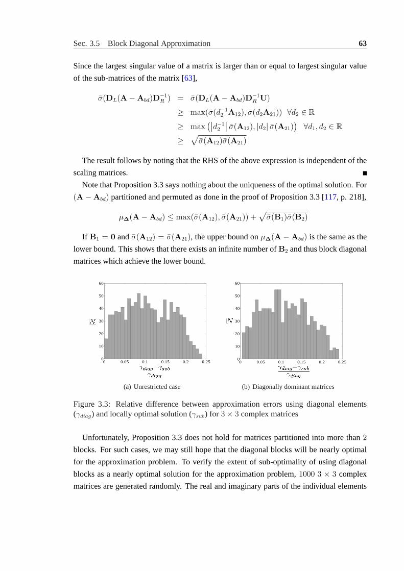
Sec. 3.5 Block Diagonal Approximation 63
Since the largest singular value of a matrix is larger than or equal to largest singular value
of the sub-matrices of the matrix [63],
σ(DL(A−Abd)D−1R ) = σ(DL(A−Abd)D
−1R U)
≥ max(σ(d−12 A12), σ(d2A21)) ∀d2 ∈ R
≥ max(∣∣d−1
2
∣∣ σ(A12), |d2| σ(A21)) ∀d1, d2 ∈ R
≥√
σ(A12)σ(A21)
The result follows by noting that the RHS of the above expression is independent of the
scaling matrices.
Note that Proposition3.3says nothing about the uniqueness of the optimal solution. For
(A−Abd) partitioned and permuted as done in the proof of Proposition3.3[117, p. 218],
µ∆(A−Abd) ≤ max(σ(A12), σ(A21)) +√
σ(B1)σ(B2)
If B1 = 0 andσ(A12) = σ(A21), the upper bound onµ∆(A −Abd) is the same as the
lower bound. This shows that there exists an infinite number ofB2 and thus block diagonal
matrices which achieve the lower bound.
0 0.05 0.1 0.15 0.2 0.250
10
20
30
40
50
60
0 0.05 0.1 0.15 0.2 0.250
10
20
30
40
50
60
(a) Unrestricted case
0 0.05 0.1 0.15 0.2 0.250
10
20
30
40
50
60
0 0.05 0.1 0.15 0.2 0.250
10
20
30
40
50
60
(b) Diagonally dominant matrices
Figure 3.3: Relative difference between approximation errors using diagonal elements(γdiag) and locally optimal solution (γsub) for 3× 3 complex matrices
Unfortunately, Proposition3.3 does not hold for matrices partitioned into more than2
blocks. For such cases, we may still hope that the diagonal blocks will be nearly optimal
for the approximation problem. To verify the extent of sub-optimality of using diagonal
blocks as a nearly optimal solution for the approximation problem,1000 3 × 3 complex
matrices are generated randomly. The real and imaginary parts of the individual elements
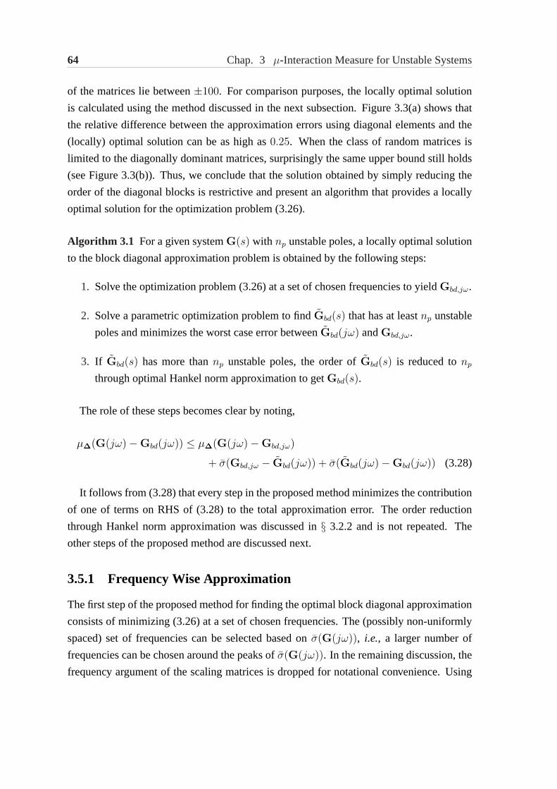
64 Chap. 3 µ-Interaction Measure for Unstable Systems
of the matrices lie between±100. For comparison purposes, the locally optimal solution
is calculated using the method discussed in the next subsection. Figure3.3(a)shows that
the relative difference between the approximation errors using diagonal elements and the
(locally) optimal solution can be as high as0.25. When the class of random matrices is
limited to the diagonally dominant matrices, surprisingly the same upper bound still holds
(see Figure3.3(b)). Thus, we conclude that the solution obtained by simply reducing the
order of the diagonal blocks is restrictive and present an algorithm that provides a locally
optimal solution for the optimization problem (3.26).
Algorithm 3.1 For a given systemG(s) with np unstable poles, a locally optimal solution
to the block diagonal approximation problem is obtained by the following steps:
1. Solve the optimization problem (3.26) at a set of chosen frequencies to yieldGbd,jω.
2. Solve a parametric optimization problem to findGbd(s) that has at leastnp unstable
poles and minimizes the worst case error betweenGbd(jω) andGbd,jω.
3. If Gbd(s) has more thannp unstable poles, the order ofGbd(s) is reduced tonp
through optimal Hankel norm approximation to getGbd(s).
The role of these steps becomes clear by noting,
µ∆(G(jω)−Gbd(jω)) ≤ µ∆(G(jω)−Gbd,jω)
+ σ(Gbd,jω − Gbd(jω)) + σ(Gbd(jω)−Gbd(jω)) (3.28)
It follows from (3.28) that every step in the proposed method minimizes the contribution
of one of terms on RHS of (3.28) to the total approximation error. The order reduction
through Hankel norm approximation was discussed in§ 3.2.2 and is not repeated. The
other steps of the proposed method are discussed next.
3.5.1 Frequency Wise Approximation
The first step of the proposed method for finding the optimal block diagonal approximation
consists of minimizing (3.26) at a set of chosen frequencies. The (possibly non-uniformly
spaced) set of frequencies can be selected based onσ(G(jω)), i.e., a larger number of
frequencies can be chosen around the peaks ofσ(G(jω)). In the remaining discussion, the
frequency argument of the scaling matrices is dropped for notational convenience. Using

Sec. 3.5 Block Diagonal Approximation 65
similar arguments as used in calculatingµ(.) (3.6),
σ(DL(G(jω)−Gbd,jω)D−1R ) ≤ γ (3.29)
⇔ D−∗R (G(jω)−Gbd,jω)∗D∗
LDL(G(jω)−Gbd,jω)D−1R ¹ γ2I (3.30)
⇔ (G(jω)−Gbd,jω)∗PL(G(jω)−Gbd,jω) ¹ γ2PR (3.31)
wherePL = D∗LDL ∈ DL, PR = D∗
RDR ∈ DR andPL,PR Â 0. Note that unlike (3.6),
(3.31) is not affine in the decision variables; however, a locally optimal solution can be
found using an iterative approach. Using the Schur complement lemma [10], (3.30) can be
equivalently expressed as,
[ −γI D−∗R (G(jω)−Gbd,jω)∗D∗
L
DL(G(jω)−Gbd,jω)D−1R −γI
]¹ 0 (3.32)
Note that for fixedDL,DR, (3.32) is an LMI in Gbd,jω. Now, a locally optimal solution
for the frequency wise approximation problem can be found by using the following iterative
algorithm for the set of chosen frequencies:
Algorithm 3.2 Select a set of frequencies{ωi}, i = 1 · · ·nω and evaluateG(jωi). Choose
convergence toleranceε and initial D0L ∈ DL, D0
R ∈ DR (e.g. D0L = D0
R = I), where
DL,DR are given by (3.19). Seti = 1.
1. Solve the convex optimization problem (3.32) for Gibd,jω by settingDL = Di−1
L and
DR = Di−1R . Let the locally optimal approximation error beγi
1.
2. Solve (3.31) for PiL,Pi
R using a bisection search method by fixingGbd,jω asGibd,jω.
Let the locally optimal approximation error beγi2. SetDi
L = (PiL)0.5, Di
R = (PiR)0.5
andi = i + 1.
3. Repeat steps1 and2 until |γi−11 − γi−1
2 | < ε.
Unlike a general BMI problem, the sequence of solutions obtained using Algorithm3.2
is guaranteed to converge. Letγi1, γ
i2, γ
i+11 be a sequence of the approximation errors. For
convergence, we only need to show thatγi1 ≥ γi
2 ≥ γi+11 . Since the individual optimization
problems to be solved in steps1 and2 of Algorithm 3.2are convex, these steps are jointly
convex if there always existsPiL,Pi
R such thatγi1 = γi
2 andGi+1bd,jω such thatγi
2 = γi+11 .
Since (3.29) ⇔ (3.32),
γi1 = σ(Di−1
L (G(jω)−Gibd,jω)(Di−1
R )−1)

66 Chap. 3 µ-Interaction Measure for Unstable Systems
With Gbd,jω = Gibd,jω, Pi
L = PiR = I is a feasible solution for (3.31). As (3.31) is
convex, the solutionPiL = Pi
R = I can be seen as the worst case solution, which achieves
γi2 = γi
1. Now, note that
(DiL(G(jω)−Gi+1
bd,jω)(DiR)−1) = Di
LG(jω)(DiR)−1 −Gi+1
bd,jω.
As Gibd,jω is a feasible solution for (3.32), which achievesγi+1
1 = γi2, the convergence to
local optima is proven.
An equally important issue is that of quality of the solution obtained using Algorithm3.2.
Since the approximation problem has multiple local minima and the converged solution
depends on the initial value, Algorithm3.2 can converge to a minima that is worse
than using the diagonal blocks. This difficulty is overcome by replacingG(jω) by
G(jω)− diag(Gii(jω)) in Algorithm 3.2and usingGsubbd,jω + diag(Gii(jω)) as the locally
optimal solution, whereGsubbd,jω is the solution obtained using the modified algorithm.
Using the same arguments as used for convergence of the sequence of solutions obtained
using Algorithm3.2, it follows that the modified algorithm always obtains a solution that is
at least as good as using the diagonal blocks. Note that replacingG(jω)− diag(Gii(jω))
can bias the algorithm to converge to a local minima close to diagonal blocks. We
use a simple approach, where the problem is solved twice usingG(jω) and (G(jω) −diag(Gii(jω))) and select the better solution. It is possible to obtain an improved solution
using the available branch and bound methods [108], but this approach is not pursued here
with the view of keeping computational requirement low and is a potential area for future
research.
3.5.2 ParametricL∞ Optimal Identification
In this section, we discuss finding a rational transfer function that explains the frequency
response data obtained using Algorithm3.2. The objective is to find the rational transfer
matrix Gbd(s) that best approximates the irrational function and has at least as many
unstable poles asG(s). It would be ideal to directly findGbd(s) that has the same number
of unstable poles asG(s), but the optimization problem becomes very involved when the
number of unstable poles is fixed. In any case,Gbd(s) can be obtained as the optimal
Hankel norm approximation ofGbd(s) as discussed in§ 3.2.2.
Traditionally, the model identification problem consists of minimizing the least square
error or theH2 norm of Gbd,jωi− Gbd(jωi). In the present case, however, it is more
appropriate to instead minimize the worst case error or theL∞ norm ofGbd,jωi− Gbd(jωi)
(cf. (3.28)). In a related context, Helmickiet al. [60] formulated the problem of identifying

Sec. 3.5 Block Diagonal Approximation 67
H∞ optimal model from frequency response data for discrete time systems. The same
authors have extended their approach to continuous time systems in [61] through a bilinear
transformation. The two-step approach of Helmickiet al. [60] consists of fitting the
frequency response data with finite impulse response (FIR) models followed by Hankel
norm approximation, which is similar to the last two steps of the method proposed here.
Over the past few years, a number of different approaches have appeared in the literature
and the current state of the art ofH∞ optimal identification can be found in [24].
In this chapter, we parameterize the class of models using transfer functions as compared
to the FIR models used by Helmickiet al.[61]. An advantage of using the transfer function
parametrization is that low order models can be identified directly in the continuous
time domain, the disadvantage being that unlike the FIR parametrization, no worst case
error bounds are available. Nevertheless, practical experience (particularly inH2 norm
minimization case) suggests that transfer function parametrization works very well. For
simplicity, Gbd(s) is identified element by element, where[Gbd(s)]ij is parameterized as:
[Gbd(s)]ij =a(s)
b(s)=
amsm + am−1sm−1 + · · · a1s + a0
bnsn + bn−1sn−1 + · · · b1s + b0
; m ≤ n
In the remaining discussion, we drop the requirement thatGbd(s) has at least as
many poles asGbd(s), as it is easily satisfied by choosing the order of the denominator
polynomials sufficiently large. Then, the parametersa0 · · · am, b0 · · · bn, are obtained by
solving,
mina0···am,b0···bn
∣∣∣∣a(jωk)
b(jωk)− [Gbd,jωk
]ij
∣∣∣∣ k = 1 · · ·nω (3.33)
Note that the objective function in (3.33) is nonlinear, but can be equivalently represented
as|b(jωk)|−1|a(jωk)− b(jωk)[Gbd,jωk]ij|. Now, we can instead minimize
|a(jωk)− b(jωk)[Gbd,jωk]ij| =√
Re(a(jωk)− b(jωk)[Gbd,jωk]ij)2 + Im(a(jωk)− b(jωk)[Gbd,jωk
]ij)2
which is easily represented as an LMI problem as follows:
mina0···am,b0···bn∈R
γ21 + γ2
2
subject to −γ21 ≤ Re (a(jωk)− b(jωk)[Gbd,jωk
]ij) ≤ γ21
−γ22 ≤ Im (a(jωk)− b(jωk)[Gbd,jωk
]ij) ≤ γ22 k = 1 · · ·nω (3.34)
As ωk → ∞, the magnitude of the polynomialsa(jωk), b(jωk) becomes unbounded.
Thus, the formulation (3.34) inherently emphasizes minimization ofγ1, γ2 at high

68 Chap. 3 µ-Interaction Measure for Unstable Systems
frequencies. The following iterative approach can be used, which does not suffers from
this limitation:
mina(i)0 ···a(i)
m ,b(i)0 ···b(i)n ∈R
γ21 + γ2
2
subject to −γ21 |b(i−1)(jωk)| ≤ Re
(a(i)(jωk)− b(i)(jωk)[Gbd,jωk
]ij) ≤ γ2
1 |b(i−1)(jωk)|−γ2
1 |b(i−1)(jωk)| ≤ Im(a(i)(jωk)− b(i)(jωk)[Gbd,jωk
]ij) ≤ γ2
2 |b(i−1)(jωk)|bn = 1 (3.35)
whereb(i−1)(jωk) denotes the identifiedb polynomial from the previous iteration. In (3.35),
the additional constraintbn = 1 is imposed for numerical stability and in general, fixing
any one of the unknown parameters suffices. In theH2 optimal identification literature,
methods similar to (3.34) and (3.35) are known as Levi’s and Sanathanan and Koerner’s
method respectively [90]. The sequence of solutions obtained by solving optimization
problem (3.35) is not guaranteed to converge, but reasonable solution can be obtained using
a few iterations.
3.6 Controller Design
With the availability ofGbd(s) using Algorithm3.1, the controller design for the modified
µ-IM is similar to the conventionalµ-IM method. A loop shaping approach can be
used to find the stabilizing decentralized controller; however, finding a controller using
this method to satisfy (3.16) can be difficult. In this section, we show that with the
alternate representation of theµ-IM conditions in terms ofKbdSbd(s), finding Kbd(s) to
satisfy (3.16) reduces to solving a weightedH∞ controller design problem forGbd(s).
Proposition 3.4 Consider thatG(s) andGbd(s) havenp unstable poles. Let the minimum
phase and stable transfer matrixw(s) be chosen such that|w(jω)| = µ−1∆ (GI(jω))
for all ω. There exists a block diagonal controllerKbd(s) such thatσ(KbdSbd(jω)) <
µ−1∆ (GI(jω)) for all ω ∈ R iff
σ−1H (U(w−1Gbd(s))
∗) < 1 (3.36)
whereU(.) denotes the unstable part.
Proof: (Sufficiency) Let us define,Kbd(s) = w(s)Kbd(s) andGbd(s) = w−1(s)Kbd(s).
Then, using Proposition2.3, there exists aKbd(s) such that,
infKbd(s)
‖wKbdSbd(s)‖∞ = infKbd(s)
‖Kbd(s)(I + GbdKbd(s))−1‖∞
= σ−1H (U(w−1Gbd(s))
∗)

Sec. 3.6 Controller Design 69
If (3.36) holds, there exists aKbd(s) such that
‖wKbdSbd(s)‖∞ < 1 (3.37)
⇔ σ(wKbdSbd(jω)) < 1 ∀ω⇔ σ(KbdSbd(jω)) < |w(jω)|−1 ∀ω⇔ σ(KbdSbd(jω)) < µ−1
∆ (GI(jω)) ∀ω
where the last inequality holds as|w(jω)| = µ∆(GI(jω)) for all ω.
(Necessity) We show the necessity of (3.36) by contradiction. Consider that (3.36) does
not hold, but there exists aKbd(s) such thatσ(KbdSbd(jω)) < µ−1∆ (GI(jω)) ∀ω. By
reversing the series of inequalities used for sufficiency,Kbd(s) must satisfy (3.37). The
σ−1H (U(w−1Gbd(s))
∗) denotes the least achievable value for‖w(s)KbdSbd(s)‖∞ for all LTI
controllers. Then,‖wKbdSbd(s)‖∞ being less than1, despiteσ−1H (U(w−1Gbd(s))
∗) being
equal to or greater than1 is a contradiction and the necessity of (3.36) follows.
In Proposition3.4, we assumed thatw(s) is stable and minimum phase. In general,w(s)
can have RHP zeros and RHP poles at same the location asGbd(s). Allowing w(s) to
be unstable or non-minimum phase provides no advantage, as following the discussion in
§ 2.3, we can simply replacew(s) by its minimum and stable part in (3.36). On relaxing this
assumption, however,w(s) that achieves|w(jω)| = µ−1∆ (GI(jω)) becomes non-unique,
where the different instances ofw(s) are related by a unitary transformation.
Proposition3.4 effectively reduces the task of finding a block decentralized controller
to satisfy µ-IM condition (3.16) to finding the minimum phase and stablew(s) such
that |w(jω)| = µ−1∆ (GI(jω)) and (3.36) holds. When (3.36) is satisfied, the standard
H∞ optimal control design techniques can be used to find the stabilizing decentralized
controller.
Remark 3.5 In practice, it can be difficult to findw(s) that satisfies|w(jω)| =
µ−1∆ (GI(jω)) for all ω ∈ R. This difficulty can be overcome by recognizing that any
w(s) that lower boundsµ∆(GI(jω)) at all frequencies, if (3.36) holds,
σ(KbdSbd(jω)) < |w(jω)|−1 ⇒ σ(KbdSbd(jω)) < µ−1∆ (GI(jω))
Thus, for a givenGbd(s) the existence of a decentralized stabilized controller can be
established by verifying (3.36) with w(s) that lower boundsµ∆(GI(jω)).
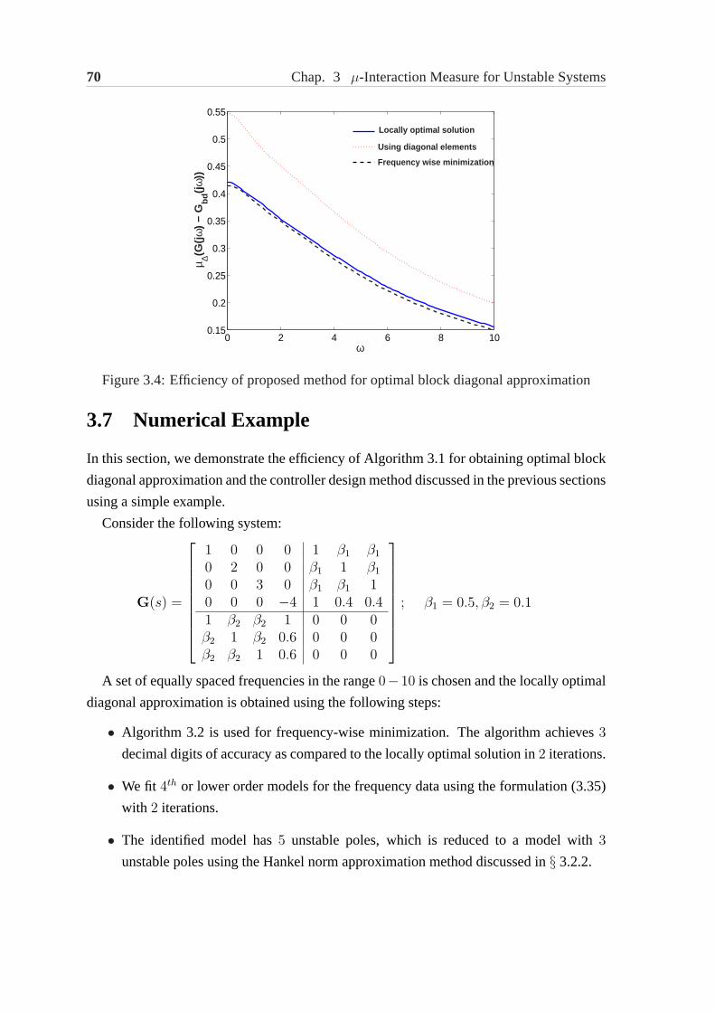
70 Chap. 3 µ-Interaction Measure for Unstable Systems
0 2 4 6 8 100.15
0.2
0.25
0.3
0.35
0.4
0.45
0.5
0.55
ω
µ ∆(G(j
ω)
− G
bd(j
ω))
Locally optimal solution
Using diagonal elements
Frequency wise minimization
Figure 3.4:Efficiency of proposed method for optimal block diagonal approximation
3.7 Numerical Example
In this section, we demonstrate the efficiency of Algorithm3.1for obtaining optimal block
diagonal approximation and the controller design method discussed in the previous sections
using a simple example.
Consider the following system:
G(s) =
1 0 0 0 1 β1 β1
0 2 0 0 β1 1 β1
0 0 3 0 β1 β1 10 0 0 −4 1 0.4 0.41 β2 β2 1 0 0 0β2 1 β2 0.6 0 0 0β2 β2 1 0.6 0 0 0
; β1 = 0.5, β2 = 0.1
A set of equally spaced frequencies in the range0− 10 is chosen and the locally optimal
diagonal approximation is obtained using the following steps:
• Algorithm 3.2 is used for frequency-wise minimization. The algorithm achieves3
decimal digits of accuracy as compared to the locally optimal solution in2 iterations.
• We fit 4th or lower order models for the frequency data using the formulation (3.35)
with 2 iterations.
• The identified model has5 unstable poles, which is reduced to a model with3
unstable poles using the Hankel norm approximation method discussed in§ 3.2.2.

Sec. 3.7 Numerical Example 71
0 2 4 6 8 101
2
3
4
5
6
7
Am
plit
u de
Figure 3.5:Validation of modifiedµ-IM for stabilizing decentralized controller designedusing independent designs
TheGsubbd (s), as obtained following these steps, is given as:
diag(−0.002s2+2.22s+3.421
s2+2.92s−3.96 , −0.01045s2+2.04s+5.98s2+2.53s−9.69 , −0.01575s2+1.842s+4.98
s2+1.77s−8.99
)
For comparison purposes, we also calculate the sub-optimal solutionGdiagbd (s) by
reducing the order of diagonal elements ofG. In this case,5 Hankel singular values of
the stable part ofGdiagbd (s) are negligible, which are removed to get a reduced order model
given as:
diag(
2.075s+3.272s2+2.96s−4.16 ,
1.33s+3.896s2+2.06s−7.762 ,
−0.006s2+1.255s+3.533s2+1.422s−10.31
)
To show the advantage of Algorithm3.1 over using diagonal elements,γsub =
µ∆(G(jω)−Gsubbd (jω)) andγdiag = µ∆(G(jω)−Gdiag
bd (jω)) are compared in Figure3.4.
The relative difference betweenγdiag and γsub is 0.23 at the zero frequency, which
monotonically reduces to0.13 for ω = 10. This significant reduction in the approximation
error is useful for finding the stabilizing controller easily. Figure3.4 also shows that the
γsub closely matches the approximation error obtained using frequency wise minimization.
Thus, (at least for this example), the conservativeness in using the two-step approach for
identifying a model, with same number of unstable poles as the system, is minimal.
Next, we consider the controller design part. For the locally optimal diagonal
approximation, the following weight approximatesµ∆(GI(jω)) closely,
w(s) =0.107s2 + 2.12s + 10.54
s2 + 2.06s + 7.762

72 Chap. 3 µ-Interaction Measure for Unstable Systems
Using this w(s), σH(U(w−1Gsubbd (s))∗) = 1.06 > 1 and standardH∞ optimal
controller design technique is used to find a decentralized stabilizing controller. The
plots of µ−1∆ (GI(jω)) and σ([Gbd(jω)]ii), i = 1, 2, 3 are shown in Figure3.5, where
µ−1∆ (GI(jω)) > σ([Gbd(jω)]ii), as expected. On the other hand, for the suboptimal
solution obtained using the diagonal elements,σH(U(w−1(s)Gdiagbd (s))∗) = 0.524 < 1.
Then, the conservativeness of using the diagonal elements to find a suboptimal solution is
emphasized.
3.8 Chapter Summary
In this chapter, we extended the practical applicability ofµ-IM to unstable systems.
The decentralized controller is designed based on a block diagonal approximation that is
different from the block diagonal elements, but has same number of unstable poles as the
system. By expressing theµ-IM in terms of transfer matrix from disturbances to inputs, it
is shown that:
• The block diagonal approximation can be (sub-optimally) chosen by minimizing the
scaledL∞ distance between the system and the approximation.
• The task of designing the controller based on the block diagonal approximation can
be reduced to solving a weightedH∞ optimal controller design problem.
• The decentralized stabilizing controller inherently minimizes an upper bound on the
input requirement for stabilization, but the bound is very loose.
We have shown that when the system is partitioned into2 blocks, the optimal block
diagonal approximation can be obtained by order reduction of diagonal blocks. For
the general case, a step-wise numerical approach is presented for finding the locally
optimal solution to the block diagonal approximation problem. The proposed approach
involves solving the approximation problem at a set of frequencies followed byL∞ optimal
identification.
One promising approach for identifying low order continuous models from frequency
response data is to use the Nevanlinna-Pick interpolation theory [6]. The interpolation
theory parameterizes all rational stable functions that can pass through the given set of
(adjusted) complex valued data. This method has been used by Chenet al. [25] for H∞optimal identification and can easily be extended to theL∞ case. The present difficulties
in using this approach are (i) the order of the model is the same as the number of data

Sec. 3.8 Chapter Summary 73
points; and more importantly, (ii) due to an over-emphasis on the given set of frequencies,
the interpolating function shows inter-sample oscillations.
The primary limitation of choosing the block diagonal approximation by minimizing the
scaledL∞ distance is that the properties of the approximant are not taken into account. As
shown in this chapter, whether the stabilizing controller can be easily found depends on
the minimum Hankel singular value of the approximation. A better approach is to use a
multi-objective optimization framework, where theL∞ distance between the system and
the approximation is minimized and simultaneously the minimum Hankel singular of the
approximation is maximized. This non-trivial problem is a topic for future work.


Chapter 4
Block Relative Gain: Properties andPairing Rules
Block relative gain (BRG) is a useful method for finding suitable pairings for block decen-
tralized control. In this chapter, we present some new algebraic properties of BRG and
establish its relation with closed loop stability, controllability, block diagonal dominance
and interactions. We show that the common conjecture that a system is weakly interacting,
if BRG is close to the Identity matrix, is not true. Based on these insights, simple rules for
pairing of variables are proposed. We also extend the known method for calculating RGA
for interacting systems to BRG.1
4.1 Introduction
Decentralized controllers are widely used in the process industries due to their simplicity.
The performance of a fully decentralized controller can be poor in presence of severe
process interactions. In such situations, the use of full multivariable controller is an
attractive alternative. On the other hand, decentralized controllers are easier to design,
tune and can be made fault-tolerant more easily as compared to full multivariable
controllers [18]. An alternative to either fully decentralized or a full multivariable controller
is the use of block decentralized controller, which has a structure in between the two
extremes. Block decentralized controllers balance the high performance given by full
multivariable controllers and the easier implementation and maintenance associated with
1This work has been published in Industrial Engineering & Chemistry Research [72] and a shorter versionin the proceedings of ADCHEM 2003, Hong Kong, P.R. China [73].
75

76 Chap. 4 Block Relative Gain: Properties and Pairing Rules
fully decentralized controllers. The use of block decentralized controllers can be further
justified by the fact that in most industrial processes, the interactions are limited in scope
and do not include the full scope of the plant. Thus, these processes are most suitably
controlled in ablock-wisefashion. Since the number of such blocks and block decentralized
alternatives increases rapidly with system size, controller design for every alternative is
impractical at design stage. Thus, effective tools are required to get an estimate of closed
loop properties without designing the actual controller. In this chapter, we present results
concerning such a tool,i.e., Block relative gain (BRG) [83].
The BRG generalizes the concept of the relative gain array (RGA) [17] to block pairings.
It is a powerful technique for input-output controllability analysis and screening alternatives
quickly for block decentralized control at the design stage. The development of the BRG is
based on the assumption of perfect control2. Arkun [3] has argued that rigorous closed loop
stability and performance analysis is not possible under this assumption and has suggested
the use of the dynamic block relative gain. The BRG has also been extended to handle
non-square [93] and non-linear [82] cases. However, the applicability of these extensions
of the BRG is limited due to their dependence upon controller tuning and their extensive
computational requirements. These approaches are not considered here and the discussion
is limited to square, linear time invariant (LTI) and stable systems, unless otherwise stated.
During the past few decades, the RGA has been studied extensively [51, 65, 71, 113]
and its properties are well understood, but the BRG has largely been overlooked. Some
researchers [20, 85] have found relations between the BRG and Euclidian condition
number. It is shown that generally, a system is difficult to control, if the maximum
singular value of BRG is large. Chenet al. [23] have further considered the role of
the BRG in robustness analysis. Despite these studies, contrary to the RGA, BRG has
not gained widespread popularity and block pairings are selected primarily based on
heuristics [19, 29]. The use of heuristics can be attributed to lack of a study showing that
similar to the RGA, information regarding closed loop properties can be obtained using
BRG. This motivates the present work.
In this chapter, we present some novel algebraic properties of BRG. We establish the
connection between BRG and closed loop properties like stability, controllability, block
diagonal dominance and interactions. Manousiouthakiset al. [83] have claimed that a
system isweakly interacting, if BRG is close to the Identity matrix and have proposed
a pairing algorithm based on this statement. We show that this claim is incorrect. Further, a
system can have large interactions despite BRG being exactly the Identity matrix. It should
2Perfect control is achieved, when the output,y(t) is equal to the reference,r(t) ∀t > 0 [102].
Sec. 4.2 Preliminaries 77
be emphasized, however, that if the singular values of BRG are very different from unity,
the closed loop system has large interactions. Based on these insights, simple rules for
variable pairing are proposed. Simultaneously, we present a note on calculation of BRG,
when the system contains integrating elements.
Grosdidieret al. [51] pointed out that modelling uncertainties and changing operating
conditions make it very difficult to develop reliable dynamic models for chemical processes
and often, only steady state gain information is available. With this motivation, we focus
on extracting useful feedback properties from gain information, though most of the results
presented are directly generalizable to higher frequencies.
The organization of this chapter is as follows. In§4.2, we revisit the development of
BRG and cite the limitations of existing pairing rules; in§4.3, we present some algebraic
properties of BRG; the main results of this chapter are contained in§4.4, where it is shown
that BRG can be used to assess some desired closed loop properties; in§4.5, alternate
pairing rules are proposed and illustrative examples are presented; in§4.6, we consider the
case, when the system matrix contains integrating elements and§4.7concludes this chapter.
4.2 Preliminaries
In this section, we introduce the concepts of relative gain and BRG. We present the BRG
based pairing rules due to Manousiouthakis [83] and point to their limitations.
As before, the transfer function matrix relating outputs and inputs of the system is
represented asG(s) in this chapter. The steady state gain matrix is represented asG(0)
or simplyG ∈ Rn×n. The objective is to decompose the original system into a set ofM
non-overlapping square subsystems such that,Gii ∈ Rmi×mi; i = 1, 2 · · ·M ,∑
i mi = n.
Gij ∈ Rmi×mj represents theijth block of G or the block gain betweenyi anduj. The
pair (yi,uj) denotes the variables related byGij(s).
Definition 4.1 Relative gain[17] for variable pairing (yi,uj) is defined as the ratio of two
gains representing first the process gain in an isolated loop and second, the apparent process
gain in the same loop when all other control loops are closed,
λij = gij
[G(0)−1
]ji
Λ(G) = [λij] = G(0) ◦G(0)−T
where◦ is the Hadamard product andG(0)−T is transpose of the inverse ofG(0). Λ(G)
is called RGA. Manousiouthakiset al. [83] extended the concept of the RGA to BRG for
synthesizing block decentralized controllers.

78 Chap. 4 Block Relative Gain: Properties and Pairing Rules
Definition 4.2 Block relative gain[83] for variable pairing (y1,u1) is defined as the ratio
of the open loop block gain and apparent block gain in the same loop when all other control
loops are closed,
[ΛB(s)]11 = G11(s)[G−1(s)]11 (4.1)
whereG11(s) is them1×m1 transfer function matrix,m1 ≤ n, relating the firstm1 inputs
and outputs ofG and[G−1(s)]11 is the corresponding block ofG−1(s).
Precisely, (4.1) represents the expression for left-BRG. Similarly, right-BRG can be
calculated as[G−1(s)]11G11(s). Since the left and right-BRG share common properties,
consideration of right-BRG is omitted from this discussion.
4.2.1 BRG Revisited
Let the LTI system,y(s) = G(s)u(s) + d(s) be conformably partitioned such thatG11(s)
is anm1 ×m1 transfer function matrix,
y1(s) = G11(s)u1(s) + G12(s)u2(s) + d(s)
y2(s) = G21(s)u1(s) + G22(s)u2(s) + d(s) (4.2)
When (y2,u2) is perfectly controlled andd(s) ≈ 0, at steady state, (y1,u1) are related
through the Schur complement ofG22 in G [102],
y1 = G11u1; G11 = G11 −G12G−122 G21 (4.3)
In (4.3), it is assumed that the subsystemG22 is nonsingular, though it is not necessary
for existence of the BRG, as is shown later. For partitioned matrices [62], [G−1]11 = G−111 .
Now, the steady state block relative gain between (y1,u1) can be defined as,
[ΛB]11 = G11[G−1]11 (4.4)
Similarly,G can also be partitioned intoM diagonal and conformal off-diagonal blocks,
such thatGii ∈ Rmi×mi; i = 1, 2 · · ·M . Then,
[ΛB]ii = Gii[G−1]ii (4.5)
Manousiouthakiset al. [83] have suggested choosing the pairings such that the
eigenvalues of all the corresponding BRGs are close to 1. This pairing rule is based on the
conjecture that a system isweaklyinteracting, if the BRG is close to the Identity matrix, and
is similar to the pairing rules for RGA prevalent then. Now, it is well known that pairing on
RGA elements close to 1 can lead to pairings with significant interactions. Since relative
gains are a special case of BRG, the utility of this rule is also limited for choosing block
pairings.

Sec. 4.3 Algebraic Properties 79
4.3 Algebraic Properties
In this section, we present some new properties of the BRG and alternative proof of
a previously known property. Some of the properties are used to establish some more
important properties of BRG in later sections, while others are of purely algebraic interest.
Property 4.1 The individual elements of[ΛB]11 ∈ Rm1×m1, βij can be alternatively
computed as the weighted sum of RGA elements as,
βij =
m1∑
k=1
gik
gjk
λjk (4.6)
Proof: From (4.4),
βij =
∑m1
k=1(−1)j+kgikdet(Gjk)
det(G)(4.7)
whereGjk is systemG with jth row andkth column deleted. Yu and Luyben [113] have
shown that,(−1)j+kdet(Gjk)
det(G)=
λjk
gjk
(4.8)
Now, (4.6) can be obtained by substituting (4.8) into (4.7).
A special case of (4.6) is seen for diagonal elements of[ΛB]11, (i = j), [83]
βii =
m1∑
k=1
λik
This property can be helpful in reducing computational load, when the BRG is to be
calculated for different decompositions of large systems.
It is known that the row and column sum of the RGA is equal to 1 [17]. In order to
extend this property to BRG, we defineI as the ensemble of them1-dimensional ordered
index sets chosen from the firstn natural numbers. For example, forn = 3 andm1 = 2,
I has the following elements:(1, 2), (1, 3) and(2, 3). Given a matrixA, everyp, q ∈ I,
define a submatrix, denoted asApq, made up of rows and columns ofA indexed byp and
q respectively.
Property 4.2 Let p, q ⊂ I. Thenyp ⊂ y, uq ⊂ u and[ΛB(Gpq)]11 is the BRG between
yp anduq. Then,
∑q⊂I
[ΛB(Gpq)]11 =m1
n
n!
m1!(n−m1)!· Im1 ∀p ⊂ I
80 Chap. 4 Block Relative Gain: Properties and Pairing Rules
Proof: Since[ΛB(Gpq)]11 = Gpq[G−1]qp, for anyp, q ⊂ I, summation over allq ⊂ I
yields∑q⊂I
[ΛB(Gpq)]11 =∑q⊂I
Gpq[G−1]qp =
Sq∑
k=1
Gpk[G−1]kp
By construction, the cardinality of the set⋃
q for all q ∈ I is (m1 ·n!)/(m1! ·(n−m1)!),
where the set⋃
q contains the firstn natural numbers repeated(m1 ·n!)/(n·m1!·(n−m1)!)
times. Now the result follows by noting that,S
q∑
k=1
Gpk[G−1]kp =
m1
n
n!
m1!(n−m1)!· Im1
A similar result can be obtained by summing right-BRG over allp ⊂ I and for any
q ⊂ I. An interesting property of BRG is seen for the case whenm1 = m2 = · · ·mM = m.
Thenm is an exact divisor ofn. Let qi be defined as
qi = {qi ⊂ I | qi
⋂qj = ∅,
⋃i
qj = {1, 2 · · ·n}} ∀i, j = 1 · · ·M, i 6= j
Then the following relation holds,∑qi⊂I
[ΛB(Gpqi)] = Im ∀p ⊂ I
Essentiallyqi’s partition the input set into smaller sets of equal dimension. Form = 1,
this result reduces to the known result for RGA.
Property 4.3 Let the gain matrix,G be scaled asGs = S1GS2. S1 = diag(s1i) and
S2 = diag(s2i), i = 1 · · ·n, are output and input scaling matrices respectively and are
real. If S1 andS2 are partitioned such thatS1 = diag(S11,S12), S2 = diag(S21,S22) and
S11,S21 ∈ Rm1×m1, then [83],
[ΛsB]11 = S11 [ΛB]11 S−1
11 (4.9)
Proof: Using (4.6) and noting thatλij is independent of scaling [17],
βsij =
m1∑
k=1
(s1igiks2k)
(s1jgjks2k)λjk =
m1∑
k=1
(s1igik)
(s1jgjk)λjk = s1iβij
1
s1j
(4.10)
Recognizing thatS−111 = diag{1/s11, 1/s12 · · · 1/s1m}, the equivalence of (4.9) and (4.10)
can be shown.
Based on (4.9) and (4.10), the following observations are made:

Sec. 4.3 Algebraic Properties 81
(i) βsij is independent of input scaling, but dependent on output scaling.
(ii) [ΛB]ii is independent of scaling of[ΛB]jj, for all i, j = 1, 2 · · ·M , j 6= i.
(iii) If all outputs are scaled by the same scalar, thenβsij = βij. This can be shown by
settings11 = s12 = · · · = s1m in (4.10).
(iv) The diagonal elements of BRG,βij, (i = j), are independent of scaling.
In the development of the BRG, it was assumed thatGii is non-singular. The next
property shows that the existence of[ΛB]ii does not depend on the fulfillment of this
assumption.
Property 4.4 If G is non-singular andGii is singular, then[ΛB]ii exists and is singular.
Proof: SinceG is non-singular by assumption,G−1 and thus[G−1]ii exists. Thus,[ΛB]ii
exists, but is rank deficient due to rank deficiency ofGii (cf. (4.5)).
Example 4.1 Consider the gain matrixG decomposed into2× 2 and1× 1 blocks,
G =
1 2 1.51 2 43 1 5
; [ΛB]11 =
(1.6 −0.61.6 −0.6
); [ΛB]22 = 0
Clearly, the first2× 2 block ofG is singular. For((y1-y2,u1-u2), (y3,u3)) pairings,[ΛB]11
exists, but is singular.
Property 4.5 For some specified partitioning of the system,
(i) G being block triangular implies that the corresponding[ΛB]ii = Imifor all i =
1 · · ·M .
(ii) [ΛB]ii = Imifor all i = 1 · · ·M does not imply thatG is block triangular.
Proof: (i) For block triangular matrices,[G−1]ii = [Gii]−1. Then, using (4.5), [ΛB]ii =
Gii[Gii]−1 = Imi
.
(ii) When only SISO pairings are used, the BRGs are the same as the diagonal elements
of RGA and the converse is proved trivially. To show that it is true for any arbitrary
partitioning, it would suffice to construct an example showing that[ΛB]ii can be the Identity
matrix for all i even whenG is not block triangular. Let the system be partitioned in
accordance to (4.2). Using (4.3) and (4.4),
[ΛB]11 = [I−G12G−122 G21G
−111 ]−1

82 Chap. 4 Block Relative Gain: Properties and Pairing Rules
If one of the pairs,{G12,G−122 G21G
−111 } and{G12G
−122 ,G21G
−111 } lie in null space of each
other, [ΛB]11 is the Identity matrix. In either case,G12 is singular. Similarly, if one of
the pairs,{G21 , G−111 G12G
−122 } and{G21G
−111 , G12G
−122 } lie in null space of each other,
[ΛB]22 is the Identity matrix. Then,G21 is singular. Clearly, it is not required that one
or both ofG12 andG21 be zero matrices orG be block triangular for[ΛB]11 = Im1 and
[ΛB]22 = Im2. Similar arguments can be used to reach this conclusion, when the system is
to be partitioned into any arbitrary number of blocks.
Example 4.2 Consider the system
G =
0.2 2 2.5 1.11.5 0.4 2.5 1.11.3 −1.6 0.5 1−1.3 1.6 2 0.1
For a2 × 2 and2 × 2 decomposition ofG, [ΛB]11 and [ΛB]22 are equal to the Identity
matrix, despite the system not being block triangular. Note that in this example, both the
off-diagonal blocks are singular.
If G is block triangular, then the system is one-way interacting. In this case, the
stability of the individual loops implies the stability of the overall system. Property4.5
shows that this cannot be inferred directly from BRG. In the context of SISO pairings,
this property relates to the diagonal elements of RGA only. Some researchers,e.g. Hovd
and Skogestad [65] (also see [102, Theorem 10.3]), have claimed that RGA being the
Identity matrix implies that the system is triangular or can be permuted to the triangular
form. By means of a counterexample, Johnson and Shapiro [71] have shown that for
G ∈ Rn×n, n ≥ 4, this is not true. Whereas the example in [71] is purely mathematical,
Braatzet al. [12] found that the RGA can be arbitrary close to the Identity matrix for real
industrial processes, which are neither triangular or can be permuted to the triangular form.
Property 4.6 If the rows and columns of the gain matrix,G are permuted such that,Gp
= P1GP2, whereP1 andP2 are permutation matrices, and further, ifP1 andP2 can be
partitioned as,
P1 =
[P11 00 P22
]P2 =
[P21 00 P22
]
then BRG for the permuted system is,
[ΛpB]11 = P11 [ΛB]11 P−1
11 (4.11)

Sec. 4.3 Algebraic Properties 83
Proof: See [83].
It should be noted that[ΛpB]11 and [ΛB]11 are equivalent from a variable pairing point
of view, as either of these represent the block gain between the same set of inputs and
outputs. Then, we may naturally seek the the total number ofdistinctblock decentralized
alternatives for a given system. This issue is addressed next by using the concept of
partition functions, but before that a formal definition of partition function is necessary.
Definition 4.3 A partition of a positive integern is a finite non-increasing sequence of
positive integersq1, q2, · · · qr, such that∑r
i=1qi = n. The partition functionp(n) is the
number of possible partitions ofn [2].
Essentially,p(n) represents the number of ways of writingn as sum of smaller integers,
where the order of the addends is not considered significant. In the present context,p(n)
represents the number of ways of block partitioning the given system.
Property 4.7 The number of distinct block decentralized alternatives,N(n) for a square
system is given by,
N(n) =
p(n)∑i=1
(n!)2
∏Mj=1(mj,i!)2aj,i!
;M∑
k=1
mk,i = n (4.12)
whereaj is the number of occurrences ofj in the sequence{m1,m2 · · ·mM}.
Proof: For any given decomposition, the total number of ways, in whichn outputs andn
inputs can be permuted isn! × n! = (n!)2. Considering that permutation within a block
gives rise to equivalent BRGs, the total number of distinct permutations decreases to,(
n!
m1!m2! · · ·mM !
)2
;M∑
k=1
mk = n
Let there existi, j such thatmi = mj, i, j ≤ M . Then, the cases where the same set
of outputs and inputs are assigned toith or jth block are the same. Let,aj represent the
number of occurrences ofj in the sequence{m1,m2 · · ·mM}. Thus, the total number of
distinct alternatives is given as,
(n!)2
∏Mj=1(mj!)2aj!
;M∑
k=1
mk = n (4.13)
Now, p(n) represents the total number of such possible decompositions (including the
fully centralized case). Thus, an expression forN(n) is realized by summing (4.13) over
p(n).

84 Chap. 4 Block Relative Gain: Properties and Pairing Rules
G11 G12 .. G1M
GM1 GM2 .. GMM
G21 G22 .. G2M……
………
…
……
yu
C11
CMM
C22 ……
k1
kM
……
k2
d
K
r-
Figure 4.1:Closed loop system with integral action controller
Note that the above expression forN(n) also includes thefully centralizedcase. For the
fully decentralizedcase,mj = 1 for all j, a1 = n andaj = 0 for all j > 1. Therefore the
number of alternatives is simplyn! (cf. (4.13)). Development of an analytical expression
for N(n) explicitly in terms ofn is beyond the scope of this thesis.N(n) for some typical
values ofn is presented in Table4.1. By evaluatingN(n) for different values ofn, n ≤ 40,
the following empirical relation can be obtained,
N(n) ≈ n!1.52 (4.14)
n P (n) n! N(n)3 3 6 164 5 24 1315 7 120 14966 11 720 224828 22 40320 9934563
10 42 3628800 9.0852×10⁹
15 176 1.3077×10¹² 2.5273×10¹⁸
Table 4.1:N(n) for some typical values ofn
In many practical situations, the maximum number of blocks or the maximum dimension
of individual blocks is constrained. Such cases can be handled using the concept of
restricted partitions. Andrews [2] provides a detailed discussion of partition theory.
4.4 Closed Loop Properties
Throughout this section, we assume that the controller has integral action to give
asymptotically zero tracking error. Then, the controllerKii(s), can be expressed as

Sec. 4.4 Closed Loop Properties 85
(ki · Imi/s)Cii(s), ki > 0 (see Figure4.1). It is further assumed thatH(s) = G(s)C(s)
is stable and proper. The primary objective is to relate BRG with some desired closed loop
properties including the following,
Definition 4.4 The systemG(s) is called to possessintegrity [18, 30], if there exists a
controllerK(s) with integral action such thatK(s) stabilizesG(s) for all K(s) ∈ KI(s),
where
KI(s) = {K(s) = εK | ε ∈ {0, 1}}
Definition 4.5 The systemG(s) is calledblock decentralized integral controllable(block-
DIC), if there exists a controllerK(s) with integral action such thatK(s) stabilizesG(s)
for all K(s) ∈ KD(s), where
KD(s) = {K = diag(εiImi)K | εi ∈ [0, 1] , i = 1, 2, · · · ,M}
A system that possess integrity remains stable with integral action in every output
channel, when any combination of loops is taken out of service. It is assumed that a
controller that fails is immediately taken out of service,i.e. the corresponding entries in the
block diagonal controller matrix are replaced by zero. The gain of the individual loops of
a block-DIC system can be reduced independently of each other (or taken out of service)
without introducing instability in the system. Note that Block-DIC is the block version of
decentralized integral controllability (DIC) [18], known for fully decentralized controllers.
4.4.1 Stability
In this section, we consider the stability of the closed loop system operating under nominal
conditions, with one or more loops open and in the presence of actuator failure. For fully
decentralized control, it is well known that a system does not possess integrity, if one or
more associated relative gains are negative. Grosdidier and Morari [50] have extended this
result to block pairings.
Lemma 4.1 Let H(s) = GC(s) be a rational proper system. With reference to Figure4.1,
assume thatk1 = k2 · · · = kM = k. Then, H(s) is closed loop stable only if
det(H(0)) > 0 [51].
Theorem 4.1 Let H(s)GC(s) be a proper system. Ifdet([ΛB(0)]ii) < 0, for somei,
i = 1, 2 · · ·M , then at least one of the following is true [50],
1. The closed loop system is unstable.
86 Chap. 4 Block Relative Gain: Properties and Pairing Rules
2. The closed loop system is unstable asith loop is removed.
3. Theith loop considered in isolation with other loops is unstable.
Proof: Using (4.5) and Schur complement lemma,det([ΛB(0)]ii) can be expanded as,
det([ΛB(0)]ii) =det(Gii(0))det(Gii(0))
det(G(0))=
det(Gii(0)Cii(0))det(Gii(0)Cii(0))
det(G(0)C(0))(4.15)
whereGii(0) is the systemG(0) with all the rows and columns corresponding to theith
loop deleted. The second equality follows sincedet(C(0)) = det(Cii(0))det(Cii(0)).
det([ΛB(0)]ii) < 0 implies that at least one of the terms in (4.15) is negative. Then, the
conclusions can be drawn using Lemma4.1.
If the individual loops are stable, then the stability of the closed loop system and the
reduced system with one of theM loops removed is assessed using Theorem4.1. It is
generalized to the case when any combination of loops are open by the following corollary.
Corollary 4.1 Let p be a subset of integers chosen from the firstM integers. Then,Gpp(0)
is a submatrix consisting of blocks ofG(0) indexed byp andyp ∈ y. For a rational proper
systemH(s), if det([ΛB(Gpp(0))]11) < 0, then at least one of the following is unstable:
1. the closed loop system or
2. the reduced system with the loops indexed byp removed (yp left uncontrolled) or
3. the reduced system with only the loops indexed byp closed (onlyyp controlled).
Though useful, when used alone, Theorem4.1 can be inadequate in some cases.
Consider the individual loops to be stable, but the closed loop system and the reduced
system withith loop removed to be unstable. In this case,det([ΛB(0)]ii) > 0 despite
the system not having integrity. This difficulty can be overcome by using Theorem4.1 in
conjunction with generalized Niederlinski index (NI).
Theorem 4.2 Let H(s)GC(s) be rational and proper. Assume that the individual loops
are stable and have vanishing tracking error. Then the closed loop system is stable only
if, [ 49]
NI =det(G(0))∏M
i=1 det(Gii(0))> 0; det(Gii(0)) 6= 0 ∀i = 1, 2 · · ·M (4.16)

Sec. 4.4 Closed Loop Properties 87
It follows from earlier discussion that a system has integrity only ifdet([ΛB(0)]ii) > 0
for all i = 1, 2 · · ·M andNI > 0. Similar to loop failure sensitivity, an equally important
issue is that of actuator failure sensitivity. A system is calledjth actuator failure sensitive
(j-AFS), if the nominal system is stable but becomes unstable if thejth actuator andjth
sensor are removed [51]. Then using Lemma4.1, a system isj−AFS if det(GjjCjj) < 0.
Note that for SISO pairings, actuator failure sensitivity and loop failure sensitivity are
equivalent. For block pairings, BRG can be used to assess the actuator failure sensitivity of
the system. We assume that the variables of the system are reordered such that1 ≤ j ≤ m1
or thejth actuator lies in the first block of the partitioned system. Then,[G11(0)]jj is the
loop gain withjth sensor andjth actuator removed.
Corollary 4.2 Let the rational proper systemH(s) and its individual loops be nominally
stable. Assume thatdet([ΛB(G(0))]11) > 0. Then, if det([ΛB(Gjj(0))]11) < 0 or
NI(Gjj(0)) < 0, at least one of the following isj−AFS: (i) the closed loop system or
(ii) the loop itself.
Proof: Similar to (4.15), det([ΛB(Gjj(0))]11) can be expanded as,
det([ΛB(Gjj(0))]11) =det([G11(0)]jj[C11(0)]jj)det(G
′11(0)C
′11(0))
det(Gjj(0)Cjj(0))
Since the nominal system and its individual loops are stable anddet([ΛB(G(0))]11) > 0,
the reduced system with first loop removed is stable,i.e. det(G′11(0)C
′11(0)) > 0.
Similarly,
NI(Gjj(0)) =det(Gjj(0))Cjj(0))
det([G11(0)]jj[C11(0)]jj)∏M
i=2 det(Gii(0))Cii(0))
Since the individual loops are stable,∏M
i=2 det(Gii(0))Cii(0)) > 0. Now, the conclusions
can be drawn using Lemma4.1.
Remark 4.1 Chiu and Arkun [30] have shown that the system has integrity only if both
BRG and NI, calculated for every possible combination of loops, are positive. For the
same purposes, Haggblom [59] has also discussed a method based on the concept of Partial
Relative Gains. Since the possible number of combinations of loops increases rapidly with
system size, use of these methods (and Corollary4.1) can be computationally expensive for
systems beyond moderate dimensions. This issue is further discussed in the next chapter.

88 Chap. 4 Block Relative Gain: Properties and Pairing Rules
Remark 4.2 The similarity between Theorem4.1 and IMC-filter stability criteria is
noteworthy. Garcia and Morari [40] have shown that a sufficient condition for stability
of a model inverse-based controller with a diagonal first order exponential filter is given by,
Re{λj(G(0)G(0)−1)} > 0; j = 1, 2 · · ·n (4.17)
whereG(s) is the nominal model of the systemG. Since,Gii(0) = [ΛB(0)]−1ii Gii(0),
[ΛB(0)]−1ii can be seen as multiplicative uncertainty in theith loop arising due to
closure of all other loops. Based on (4.17), the ith loop can be stabilized if
Re{λj(Gii(0)Gii(0)−1)} = Re{λj([ΛB(0)]ii)} > 0. Thus, a necessary (but not
sufficient) condition for individual loop stability isdet([ΛB(0)]ii) > 0, which is similar
to Theorem4.1. However, interpretation of BRG as multiplicative uncertainty is justified
only if the effect of hidden feedback loops is small, which is not generally true.
4.4.2 Input Output Controllability
It is well known that right half plane (RHP) zeros close to the origin pose a limitation on
the achievable output performance of the closed loop system. It is also possible thatGii(s),
considered in isolation, contains RHP zeros. The zeros ofGii(s) can limit the achievable
output performance, when the individual loops are designed independently. Skogestad
and Hovd [65] have shown that the frequency dependent RGA can be used to detect the
presence of RHP zeros (Theorem 1 in their paper). The applicability of their result is
limited to the individual elements and(n− 1)× (n− 1) dimensional subsystems ofG(s).
The next proposition complements their result for subsystems having different dimensions.
Proposition 4.1 Consider a stable transfer function matrixG(s) and its partition in
accordance to (4.2). Then [ΛB(s)]11 would be anm1 × m1 transfer function matrix. If
there existsm1, 2 ≤ m1 ≤ n − 2, such thatdet([ΛB(j∞)]11) is nonzero, finite and has a
different sign fromdet([ΛB(0)]11) , then at least one of the following is true,
(a) The subsystemG11 has a RHP zero.
(b) The subsystemG22 has a RHP zero.
Proof: For a given partitioning of the system,2 ≤ m1 ≤ n − 2, consider that
lims→j∞ det([ΛB(s)]11) is nonzero and finite. If the signs ofdet([ΛB(0)]11) andlims→j∞det([ΛB(s)]11) are different, then there exists a frequencyωo, ωo > 0, such that
det([ΛB(jωo)]11) = 0.

Sec. 4.4 Closed Loop Properties 89
The equality,det([ΛB(s)]11) = 0, is satisfied, iff one or both ofdet(G11(jωo)) and
det(G−111 (jωo)) are zero. Now,det(G11(jωo)) being zero implies the presence of a RHP
zero inG11(s) at that frequency.
If det(G−111 (jωo)) = 0, thenG−1
11 (s) contains an RHP zero andG11(s) contains an RHP
pole at that frequency. Due to stability assumptions, an RHP pole inG11(s) ats = jωo can
arise only due to an RHP zero inG22(s) ats = jωo.
This result is equally valid, ifm1 = 1 or n − 1. Then,G11(s) or G22(s) are single
elements ofG(s). In this case, if the condition imposed by Proposition4.1is satisfied, one
or both ofG11(s) andG22(s) will contain RHP zero. The BRG is input scaling independent
(see Property4.3). Thus, if an input channel ofG(s) contains an RHP zero, the signs
of det([ΛB(j∞)]11) anddet([ΛB(0)]11) will remain unchanged. The change of sign of
det([ΛB(s)]11) is only a sufficient, but not a necessary condition for the presence of RHP
zeros in the subsystems ofG(s).
Corollary 4.3 Consider thatG22(s) contains a RHP zero. If all loops but(y1(s),u1(s))
are closed, then the open loop subsystem(y1(s),u1(s)) or G11(s) contains a RHP pole.
If a RHP pole appears in the (y1(s),u1(s)) loop due to closure of all other loops, any small
disturbance in that open loop can destabilize the system. In practice, however, the gain of
the loop would remain finite due to presence of physical constraints.
Proposition4.1excludes the case in which any of the subsystems contain a zero at origin,
(s = 0). Should a subsystem contain a zero at the origin, it would be extremely difficult
to control the system. The relation between zeros at origin and the steady state BRG is
established in the next corollary.
Corollary 4.4 If there existsm1, {m1 = 1, · · · , n−1}, such thatdet([ΛB(0)]11) = 0, then
one or both of the subsystems,G11(s) andG22(s) contain a zero or a zero at the origin.
Either of these conditions is highly undesirable because it makes the system
uncontrollable. The system may also contain zeros close to the origin in the open LHP.
The presence of such poorly damped zeros also affect the system’s controllability. In such
cases, the gain of the individual loops increases considerably with closure of all other loops.
The gain of a multivariate system depends on the input direction. Let the gain of
(y1(s),u1(s)) be ‖G11(0)v‖2, ‖v‖2 = 1. Similarly, let the apparent gain of this loop,
when all other loops are closed be‖G11(0)w‖2, ‖w‖2 = 1.

90 Chap. 4 Block Relative Gain: Properties and Pairing Rules
Proposition 4.2 The worst case gain mismatch betweenG11(0) andG11(0) is bounded as
follows,
σ([ΛB(0)]11) ≤ max‖v‖2=1‖w‖2=1
‖G11(0)v‖2
‖G11(0)w‖2
(4.18)
1
σ([ΛB(0)]11)≤ max
‖v‖2=1‖w‖2=1
‖G11(0)w‖2
‖G11(0)v‖2
(4.19)
Proof: For (4.18),
max‖v‖2=1‖w‖2=1
‖G11(0)v‖2
‖G11(0)w‖2
=σ(G11(0))
σ(G11(0))= σ(G11(0))σ(G−1
11 (0))
≥ σ([ΛB(0)]11)
For (4.19),
max‖v‖2=1‖w‖2=1
‖G11(0)w‖2
‖G11(0)v‖2
=σ(G11(0))
σ(G11(0))= σ(G11(0))σ(G−1
11 (0)) ≥ σ([ΛB(0)]−111 )
≥ 1
σ([ΛB(0)]11)
Proposition4.2suggests that if at least one of the following conditions,σ([ΛB(0)]11) À 1
andσ([ΛB(0)]11)¿ 1, is satisfied, then the gain ofy1(s)−u1(s) loop changes considerably
due to closure of all other loops. Ifσ([ΛB(0)]11) ≈ 1 andσ([ΛB(0)]11) ≈ 1, the change
in gain may still be large, as (4.18) and (4.19) are lower bounds on the worst case gain
mismatch with one of the loops open. This affirms our earlier assertion that if the BRG is
far from the Identity matrix, the system has large interactions, but the converse is not true.
This is further discussed in§4.4.4.
4.4.3 Block Diagonal Dominance
When the system is block diagonal or triangular, the individual controllers can be tuned
independently of each other (Property4.5); however, most real systems do not lie in this
class. Independent tuning of individual controllers to give stable closed loop response is
still possible, if the effect ofui on yi is large compared to the effect ofuj, (i 6= j). The
concept of block diagonal dominance can be used to assess this property of the partitioned
system.

Sec. 4.4 Closed Loop Properties 91
Definition 4.6 A matrix Z is generalized row block diagonal dominantfor a given
partitioning if there existsx ∈ RM , x > 0 such that [78],
‖ Z−1ii ‖−1 xi >
M∑
j=1,j 6=i
‖ Zij ‖ xj; i = 1, 2, · · · , M
Generalized column block dominance is defined similarly. Ifx can be chosen as1Tn , then
Z is called row (column) block dominant. IfZ is generalized block diagonal dominant
(GBDD), there exists a scaling matrix of the formX = diag(xiImi), i = 1, 2 · · ·M such
thatXZX−1 is block diagonal dominant [78].
Limbeer [78] has shown that if(In + GK(s)) is GBDD for all s, then the stability
of individual loops implies the stability of the closed loop system. When the controller
contains integral action,In + (1/s)H(s) ≈ (1/s)H(s) at low frequencies [65]. At these
frequencies, the diagonal dominance of(In + (1/s)H(s)) can be assessed from diagonal
dominance ofH(s). In addition, if a system is GBDD at steady state, it is also block-DIC,
as shown next. Here,p is an ordered subset of integers chosen within the set{1, 2, · · ·M}andI is the ensemble of all possiblep’s. Then,Gpp(0) is a submatrix consisting of blocks
of G(0) indexed byp.
Lemma 4.2 Let H(s) be a proper system and the matrixD ∈ Rn×n be defined as
D = diag(diImi), di > 0. Then,G(s) is block-DIC, iff there exists a block diagonal
matrixC(0) such that
Re{λj([DH(0)]pp)} > 0 ∀j, ∀p ∈ I
Proof: Campo and Morari [18] have shown that a similar condition is necessary and
sufficient for a system to be DIC. This lemma can be shown to be true following their
proof.
Proposition 4.3 LetH(s) be a proper stable system. IfH(0) is block diagonally dominant,
thenG(s) is block-DIC.
Proof: With reference to Figure4.1, let Gii(s)Kii(s) = (ki/s · Imi)Hii(s). The ith loop
will be stable iff any of the characteristic loci of(ki/s)Hii(s) does not encircle the point
(−1/ki, 0), ass traverses the Nyquist D-contour. SinceHii(s) is stable by assumption,
such an encirclement can occur only due to the pole at the origin. Grosdidieret al. [51]
have shown that aski → 0, thejth characteristic loci does not cross the negative real axis
if Re{λj(Hii(0))} > 0; j = 1, 2 · · ·mi.

92 Chap. 4 Block Relative Gain: Properties and Pairing Rules
For a block diagonal dominant system, the total number of encirclements are same as the
sum of encirclements by individual loops [78]. Then ,Re{λj(H(0))} > 0; j = 1, 2 · · ·n,
if
Re{λj(Hii(0)} > 0; ∀j = 1, 2 · · ·mi, ∀i = 1, 2 · · ·M (4.20)
Note thatHpp(0) is block diagonal dominant due to block diagonal dominance ofH(0)
for all p ∈ I. ThenRe{λj([DH(0)]pp)} > 0 for all p ∈ I and the system is block-DIC,
if (4.20) is satisfied. For a block diagonal dominant system, (4.20) can always be satisfied
by choosingCii(0) = G−1ii (0), where the invertibility ofG−1
ii (0) is guaranteed by block
diagonal dominance.
In order to verify the generalized block diagonal dominance ofHii(0), knowledge of the
compensator matrixCii(0) is required, which can be limiting for practical purposes. We
show that whetherHii(0) is GBDD, can be assessed using BRG, which is independent of
the compensator matrix. Though the following results are valid for any matrix norms, we
use the induced2-norm due to their frequent use in the process control literature.
Lemma 4.3 Let Z be GBDD. Then [78],
σ([Z−1
]ii) ≥ σ(
[Z−1
]ji) ∀i 6= j
Proposition 4.4 The systemH(s) is GBDD only if
σ([ΛB(0)]ii) > 0.5 ∀i = 1, 2 · · ·M (4.21)
Proof: This proposition is proved using the following logical identity: IfA ⇒ B, then not
B ⇒ notA. If H(0) is a block diagonal dominant matrix
σ(Hii(0)) >M∑
j=1,j 6=i
σ(Hij(0))
Then, using Lemma4.3,
σ(Hii(0))σ([H−1(0)
]ii) >
M∑
j=1,j 6=i
σ(Hij(0))σ([H−1(0)
]ji)
σ(Hii(0)[H−1(0)
]ii) >
M∑
j=1,j 6=i
σ(Hij(0)[H−1(0)
]ji)
σ(Gii(0)[G−1(0)
]ii) >
M∑
j=1,j 6=i
σ(Gij(0)[G−1(0)
]ji) (4.22)
Sec. 4.4 Closed Loop Properties 93
Consider that multiplication ofG(0) with G−1(0),
M∑j=1
Gij(0)[G−1(0)
]ji
= Imi
σ(Gii(0)[G−1(0)
]ii) +
M∑
j=1,j 6=i
σ(Gij(0)[G−1(0)
]ji) ≥ 1
Then, using the definition of BRG (4.5) and (4.22), H(0) is block diagonal dominant
only if σ([ΛB(0)]ii) > 0.5 ∀i = 1, 2 · · ·M . Since BRG is independent of scaling of the
form X = diag(xiImi) (see property4.3), (4.22) is necessary for the system to be GBDD.
Ohtaet al. [88] have pointed out that in many cases, GBDD can be a very conservative
test for block diagonal dominance and have instead suggested the use of quasi-block
diagonal dominance (QBDD). They have shown that if(In + GK(s)) is QBDD for all
s, then the stability of individual loops implies the stability of the closed loop system. In
the following discussion, QBDD is defined formally and it is shown that the condition
σ([ΛB(0)]ii) > 0.5 for all i = 1, 2 · · ·M is necessary for a system to be QBDD.
Definition 4.7 A matrix Z is quasi-block diagonal dominantfor a given partitioning if
there existsx ∈ RM such that,
xi >
M∑
j=1,j 6=i
‖ ZijZ−1ii ‖ xj; i = 1, 2, · · · ,M ; Zii 6= 0
Corollary 4.5 The systemH(s) is QBDD only if σ([ΛB(0)]ii) > 0.5 for all i = 1, 2 · · ·M .
Proof: At low frequencies,(In + (1/s)H(s)) ≈ (1/s)H(s). Then,Hij(0)H−1ii (0) =
Gij(0)G−1ii (0). When the compensator matrix is chosen asCii = G−1
ii (0), i = 1, 2 · · ·M ,
GBDD and QBDD are equivalent (by definition). Then, using Proposition4.4, H(0) is
QBDD only if σ([ΛB(0)]ii) > 0.5, for all i = 1, 2 · · ·M .
Let E(s) = (H(s)Hbd(s)−1 − In) = (G(s)Gbd(s)
−1 − In), whereHbd(s) andGbd(s)
are matrices containing the block diagonal elements ofH(s) andG(s) respectively (see
Figure4.2). Ohtaet al. [88] have shown that if theH(s) is QBDD, there exists a norm
such that‖ XE(s)X−1 ‖< 1, whereX is the scaling matrix, defined as before. LetX be
the set defined as
X = {X ∈ Rn×n | Xii = diag(xi · Imi)} i = 1, 2 · · ·M
94 Chap. 4 Block Relative Gain: Properties and Pairing Rules
Then, with the choice of induced2−norm, the following relation holds,
µ∆(E(s)) ≤ infX∈X
σ(XE(s)X−1) σ(∆) ≤ 1
whereµ∆(.) is the structured singular value. The structure of∆ can be chosen to be
the same as that ofGbd(s), since everyX ∈ X commutes with∆, i.e. X∆ = ∆X.
Then (with the choice of induced2−norm), the systemH(s) is QBDD or GBDD only if
µ∆(E(0)) < 1. Note that this condition is also sufficient for block diagonal dominance of
the system at steady state.
In a related context, Grosdidier and Morari [49] definedµ∆(E(s)) as theµ-IM to assess
the closenessof G(s) and Gbd(s). They have shown that ifµ∆(E(0)) > 1, a block
diagonal controller with integral action cannot be designed for the given system. For fully
decentralized control, Braatz [11] has shown that a system is DIC, ifµ∆(E(0)) < 1. This
result can be easily extended to the block decentralized controllers. Whereas a pairing
alternative that satisfies theµ interaction condition is guaranteed to have some attractive
properties, the computational load for the calculation ofµ is large [15, 39]. Noting that for
all X ∈ X , Xii[ΛB(0)]iiX−1ii = [ΛB(0)]ii (see Property4.3), the following useful result is
obtained:
Corollary 4.6 For a proper systemG(s), µ∆(E(s)) < 1 only if σ([ΛB(0)]ii) > 0.5 for all
i = 1, 2 · · ·M .
For fully decentralized control, the necessary conditionσ([ΛB(0)]ii) > 0.5 reduces to
λii > 0.5 for all i = 1, 2 · · ·M . Grosdidier and Morari [49] have shown this result to be true
for 2 × 2 systems and Corollary4.6can be seen as generalization of this result to systems
with higher dimensions and block decentralized controllers. Corollary4.6can be used for
pre-screening the alternatives for pairings, reducing the computational load significantly.
4.4.4 Closed Loop Interactions
In Figure4.2, if G(s) = Gbd(s), the system is triviallynon-interacting. In this section, such
a system is referred to as anideal system. When the controller contains integral action, at
low frequencies, the sensitivity functions of the actual and the ideal systems are related
as [102],
S(s) ≈ Sbd(s)Γ(s)
S(s) = (In + G(s)K(s))−1
Sbd(s) = (In + Gbd(s)K(s))−1

Sec. 4.4 Closed Loop Properties 95
yuK11
KMM
K22 ……
d
r-
0 G12 .. G1M
GM1 GM2 .. 0
G21 0 .. G2M……
………
…
……
G11
GMM
G22 ……
Figure 4.2:Decomposition of system into block diagonal and off-block diagonal elements
whereΓ(s) = Gbd(s)G−1(s) is the Performance Relative Gain Array (PRGA) [65]. Γ(s)
can be interpreted as a filter that amplifies and rotates the exogenous signals. This action
prevents the actual system from behaving as the ideal system. LetΓ(s) be expressed
through its singular value decomposition as,Γ(s) = U(s)Σ(s)VT (s). Then,
Γ(s)vi(s) = σi(s)ui(s), ∀i = 1, 2 · · ·n
whereσi(s) is the ith singular value andui(s) andvi(s) are the corresponding left and
right singular vectors, calculated at a particular frequency. Grosdidier [48] has argued that
the exogenous signals oriented in the direction of singular vectors associated withσ(Γ(s))
most adversely affect the closed loop performance. Then, for minimization of worst case
performance loss, we may require thatσ(Γ(s)) be minimum in the desired frequency range.
Similarly, a necessary condition for interactions to be minimum is thatσi(Γ(s)) ≈ 1, for
all i = 1, 2, · · ·n in the desired frequency range. If this happens, then at every frequency,
Γ(s) is close to a unitary matrix; however,
maxi{σ([ΛB(s)]ii)} ≤ σ(Γ(s)) i = 1, 2, · · ·M (4.23)
Therefore, ifσ([ΛB(0)]ii)À 1, for all i = 1, 2, · · ·M , thenσ(Γ(0))À 1. When[ΛB(0)]ii
= I, then σj([ΛB(0)]ii) = 1, for all i = 1, 2, · · ·M ,j = 1, 2, · · ·mi. Then, (4.23)
suggests thatσ(Γ(0)) can still be large, despite the BRG being precisely the Identity matrix.
Based on these observations and Proposition4.2, we conclude that the system has large
interactions, ifσ([ΛB(0)]ii) À 1 andσ([ΛB(0)]ii) ¿ 1 or in other words,BRG is very
different from Identity, but the converse is not true. Thus, use of the PRGA is necessary for

96 Chap. 4 Block Relative Gain: Properties and Pairing Rules
drawing any conclusions regarding closed loop interactions. In some cases, this measure
can be conservative, as it does not take the directional information ofSbd into account.
Remark 4.3 The requirement thatσi(Γ(s)) ≈ 1 for low interactions is equivalent to
minimization of∑
i |σi(Γ(s))− 1|. In most of cases, it is seen that∑
i |σi(Γ(s))− 1| ≈σ(Γ(s)). Let the norm of exogenous signals be bounded from above by 1. Then for the
feedback to be effective, we require thatσ(S(s)) < 1 in the desired frequency range,
which is lower bounded byσ(Sbd(s))σ(Γ(s)) at low frequencies. Then,σ(S(s)) < 1 only
if σ(Sbd(s))σ(Γ(s)) < 1 or σ(I + Gbd(s)K(s)) > σ(Γ(s)). This inequality can be easily
satisfied by choosing a controller with low gain ifσ(Γ(s)) is small. Large controller gains
may present operational difficulties in presence of input constraints.
4.5 Alternate Pairing Rules
In earlier sections, it was shown that useful information regarding many closed loop
properties can be extracted using the BRG. In this section, we summarize those results
in the form of pairing rules.
Pairing Rule 1 Avoid pairing on variables, withdet([ΛB(0)]ii) ≤ 0 for somei or NI < 0,
otherwise the system does not have integrity (See Theorems4.1,4.2and Corollary4.4).
Pairing Rule 2 Prefer pairing on variables for whichµ∆(E(0)) < 1. Alternatives
satisfying this condition are decoupled at low frequencies and a block decentralized
controller with integral action can be designed easily (See§4.4.3). The associated
computational load can be reduced by pre-screening alternatives such thatσ([ΛB(0))]ii
> 0.5 for all i (See Proposition4.4and Corollary4.6).
Pairing Rule 3 Prefer pairing on variables for whichJ(0) =∑
i |σi(Γ(0))− 1| is small.
If J(0) is small, then the system isweaklyinteracting and vice versa, at least at steady state
(See§4.4.4).
These rules are based on gain information only and may suggest inferior pairings
for systems containing large time delays. In such cases, if a reliable dynamic model
is available, then ensuring thatJ(s) =∑
i |σi(Γ(s))− 1| is small up to the crossover
frequency is helpful. In addition,
Pairing Rule 4 Avoid pairing on variables with different signs ofdet([ΛB(0)]ii) and
det([ΛB(j∞)]ii). If the signs are different, then theith loop or the remaining subsystem
contains an RHP zero (See Proposition4.1).
Sec. 4.5 Alternate Pairing Rules 97
Remark 4.4 Since BRG and PRGA are output scaling dependent, so are their singular
values. Therefore, prior to pairing selection, specification of a suitable scaling of the system
matrix is necessary to avoid ambiguity. Some possible approaches are to normalize the
system matrix such that‖yi‖2 ≤ 1 or |yi| ≤ 1.
Remark 4.5 These pairing rules equally hold for fully decentralized control structures.
For many problems,∑
i |σi(Γ(0))− 1| is small, if the diagonal elements of RGA elements
are close to 1. Thus, Bristol’s rule of pairing on RGA elements close to 1 is implicit here,
but, in general, it is neither necessary nor sufficient for the system to be weakly interacting.
Remark 4.6 Often,∑
i |σi(Γ(0))− 1| approaches zero monotonically as the controller
structure approaches thefully centralizedcase. In such cases, a balance should be made
between the closed loop performance and the controller complexity. If a more complex
controller structure shows no significant performance improvement, then the simpler
structure (closer to thefully decentralizedcase) should be preferred.
4.5.1 Numerical Examples
Example 4.3 Consider the4× 4 ALSTOM gasifier system [32]. The gasifier is described
by three linearized state space models of25th order at100%, 50% and0% load conditions.
Prior to pairing selection, the system is scaled. The scaling procedure and the scaled gain
matrices are given in the Appendix4.A.
Various alternatives are screened at different load conditions. The analysis suggests that
((1− 2− 4, 1− 3− 4), (3− 2))3 is the only alternative, which satisfies Rules1 and2 at all
load conditions. Sinceµ∆(E(0)) < 1 for this alternative, the blocks are decoupled at low
frequencies and a controller with integral action can be designed easily.
This system has also been analyzed by Chin and Munro [29] at 100% load conditions,
where they have suggested the use of((1−3−4, 2−3−4), (2−1)). This alternative satisfies
Rules1 and2 at100% load conditions, but the relative gain of the pairing(2−1) is negative
at 0% load conditions. This shows that this alternative will lose integrity under varying
operating conditions. Though Chin and Munro [29] have scaled the system differently, it
has no effect on the conclusions, sincedet([ΛB]ii) is independent of scaling.
Example 4.4 In most of the case studies, we have found steady state analysis to be
sufficient, but in some cases it may suggest inferior pairings, as shown here. Alatiqi and
3((1− 2− 4, 1− 3− 4), (3− 2)) represents((y1 − y2 − y4, u1 − u3 − u4), (y3, u2)) variable pairing.
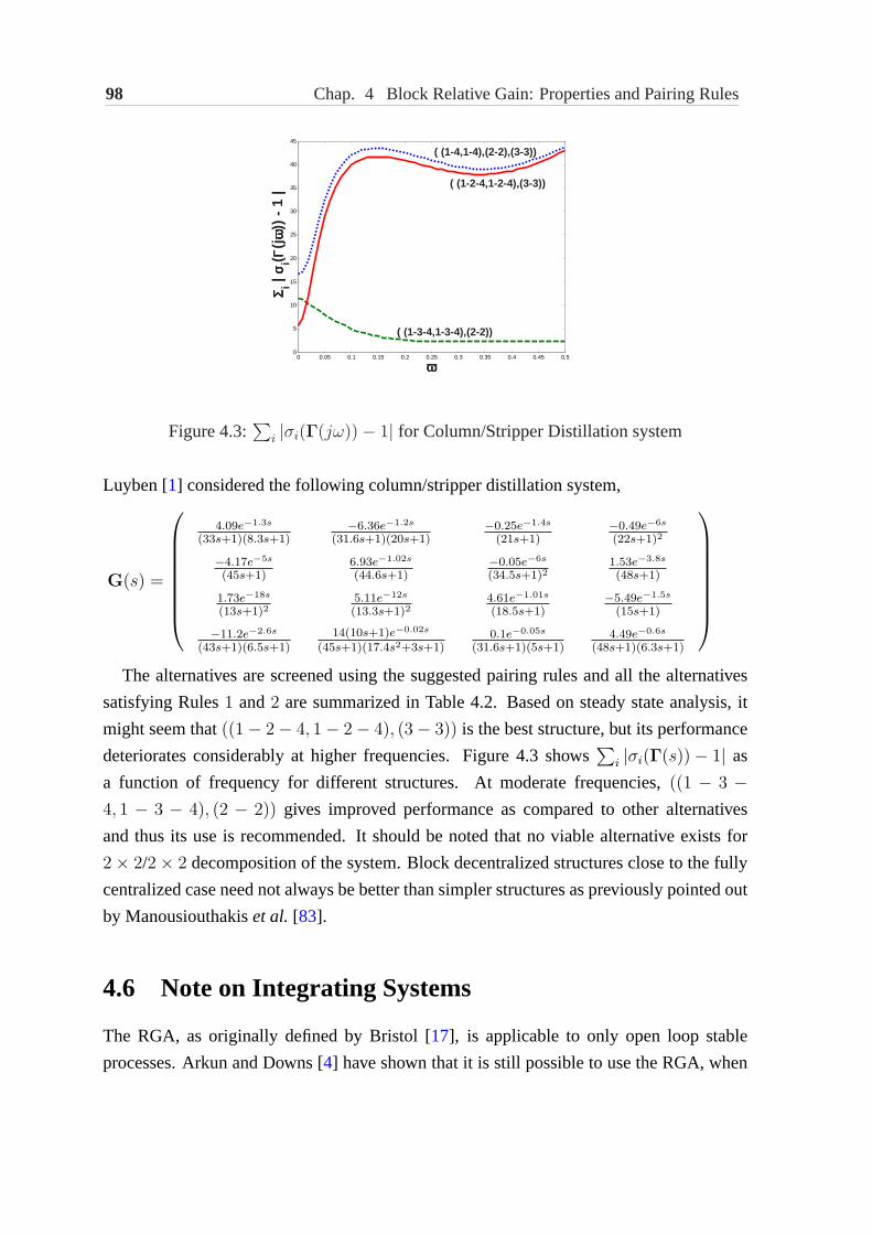
98 Chap. 4 Block Relative Gain: Properties and Pairing Rules
0 0.05 0.1 0.15 0.2 0.25 0.3 0.35 0.4 0.45 0.50
5
10
15
20
25
30
35
40
45
ωωωω
ΣΣΣΣ i | σσ σσ i( ΓΓ ΓΓ
(jωω ωω
)) -
1 |
( (1-3-4,1-3-4),(2-2))
( (1-2-4,1-2-4),(3-3))
( (1-4,1-4),(2-2),(3-3))
Figure 4.3:∑
i |σi(Γ(jω))− 1| for Column/Stripper Distillation system
Luyben [1] considered the following column/stripper distillation system,
G(s) =
4.09e−1.3s
(33s+1)(8.3s+1)−6.36e−1.2s
(31.6s+1)(20s+1)−0.25e−1.4s
(21s+1)−0.49e−6s
(22s+1)2
−4.17e−5s
(45s+1)6.93e−1.02s
(44.6s+1)−0.05e−6s
(34.5s+1)21.53e−3.8s
(48s+1)
1.73e−18s
(13s+1)25.11e−12s
(13.3s+1)24.61e−1.01s
(18.5s+1)−5.49e−1.5s
(15s+1)
−11.2e−2.6s
(43s+1)(6.5s+1)14(10s+1)e−0.02s
(45s+1)(17.4s2+3s+1)0.1e−0.05s
(31.6s+1)(5s+1)4.49e−0.6s
(48s+1)(6.3s+1)
The alternatives are screened using the suggested pairing rules and all the alternatives
satisfying Rules1 and2 are summarized in Table4.2. Based on steady state analysis, it
might seem that((1− 2− 4, 1− 2− 4), (3− 3)) is the best structure, but its performance
deteriorates considerably at higher frequencies. Figure4.3 shows∑
i |σi(Γ(s))− 1| as
a function of frequency for different structures. At moderate frequencies,((1 − 3 −4, 1 − 3 − 4), (2 − 2)) gives improved performance as compared to other alternatives
and thus its use is recommended. It should be noted that no viable alternative exists for
2× 2/2× 2 decomposition of the system. Block decentralized structures close to the fully
centralized case need not always be better than simpler structures as previously pointed out
by Manousiouthakiset al. [83].
4.6 Note on Integrating Systems
The RGA, as originally defined by Bristol [17], is applicable to only open loop stable
processes. Arkun and Downs [4] have shown that it is still possible to use the RGA, when

Sec. 4.7 Chapter Summary 99
Pairing mini(σ([ΛB(0)]ii)) µ∆(E(0))
∑i |σi(Γ(0))− 1|
(1-4,1-4),(2,2),(3,3) 1.19 0.96 16.59(1-2-4,1-2-4),(3-3) 1.19 0.53 5.65(1-3-4,1-3-4),(2-2) 0.92 0.94 11.52
Table 4.2:Alternatives for decentralized control of Column/Stripper Distillation system
the system contains integrating elements in one or more input or output channels. In such
cases, the RGA is calculated by replacing the elements containing the integrators by their
derivatives. Here, we investigate the applicability of this approach for the BRG.
Case I:Consider the case, when one or more input channels (columns ofG(s)) contain
integrator. Then, the system matrix can be partitioned into non-integrating (GNI(s)) and
integrating (GI(s)) blocks as,
G(s) =[
GNI(s)1sGI(s)
]=
[GNI(s) GI(s)
] [I 00 1
sI
](4.24)
If the second block in (4.24) is treated as a scaling matrix, then[ΛsB(0)]ii = [ΛB(0)]ii
(Property4.3(i)). In this case, it would be possible to select block pairings such that the
individual blocks contain both integrating and non-integrating elements.
Case II: Now, consider the case, when one or more output channels (rows ofG(s))
contain integrators. Partitioning the system matrix as before,
G(s) =
[GNI(s)1sGI(s)
]=
[I 00 1
sI
] [GNI(s)GI(s)
](4.25)
Here, any meaningful results can be obtained only if all the outputs containing
integrators are paired together (Property4.3(iii)) or if paired separately, only SISO pairing
is used for them (Property4.3(ii)). No block pairing should contain both non-integrating
and integrating elements.
4.7 Chapter Summary
In this chapter, we revisited the established concept of block relative gain (BRG). The main
contributions of this chapter include
(i) Extension of algebraic properties known for RGA to BRG.
(ii) Connection between the BRG and measures of block diagonal dominance, in
particular Grosdidier’sµ interaction measure [49] (see§4.4.3).

100 Chap. 4 Block Relative Gain: Properties and Pairing Rules
(iii) Correction and restatement of the common conjecture that a system isweakly
interacting, if BRG is close to Identity (see§4.4.4).
Most of the results presented are based on steady state gain information only and are
useful for controllability analysis and pairing selection. It is also shown that in some cases,
steady state analysis may suggest inferior pairings. However, practical considerations
justify its use, as in many cases, the only reliable information available at design stage
is the steady state gain. Block decentralized controllers allow the designer to exploit a
broader class of control structures that are not restricted to the two extremes of complete
decentralization and complete centralization [83]. The pairing rules proposed in this paper
will be helpful in bridging the gap between theory and practice of selection of block
pairings.
4.A Scaled Gain Matrices for ALSTOM Gasifier System
The system is scaled such that‖yi‖ ≤ 1 at all load conditions. The scaling matrix
X is chosen such thatXii = max{‖[G100%(0)]i‖2, ‖[G50%(0)]i‖2, ‖[G0%(0)]i‖2}, where
[G100%(0)]i is the ith row of the gain matrix at100% load conditions. Then,X =
diag(8.58× 10⁵, 5.21× 10⁴, 1.55× 10⁴, 164.64) and the scaled gain matrices are obtained
asGs(0) = X−1G(0).
Gs100%(0) =
0.0385 −0.0427 0.0444 −0.0474−0.1115 −0.0297 0.0770 −0.01420.0327 0.8630 0.0477 0.50190.0088 0.1284 −0.1101 −0.2834
Gs50%(0) =
0.0975 −0.0381 0.0269 −0.1130−0.2096 −0.0500 0.1563 −0.02110.0506 0.6923 0.0295 0.42000.0359 0.1804 −0.1641 −0.3967
Gs0%(0) =
0.7938 0.1451 −0.4361 −0.3983−0.7641 −0.1810 0.6161 −0.06060.0958 0.3855 −0.0301 0.25360.3119 0.3666 −0.4841 −0.7307

Chapter 5
Integrity of Systems underDecentralized Integral Control
A multivariate system has integrity if the block decentralized controller with integral action
maintains closed loop stability in presence of possible controller failures. In this chapter,
we show that the recently proposed necessary and sufficient conditions [52] for the system
to possess integrity can be equivalently expressed in terms of well-known notions of block
relative gain (BRG) [83] and Niederlinski index (NI) [87]. These results imply that the con-
ditions based on BRG and NI, traditionally believed to be only necessary, are actually both
necessary and sufficient. It is also shown that in general, establishing the existence of a fully
decentralized controller with integral action such that the system has integrity is NP-hard.
5.1 Introduction
This chapter deals with reliable stabilization of stable linear systems using a decentralized
controller with integral action in every channel. A system is said to possess integrity, if
the closed loop stability is maintained with integral action in every output channel, when
any combination of the individual controllers fails (see Definition4.4). It is assumed that
a controller that fails is immediately taken out of service,i.e. the corresponding entries
in the block diagonal controller matrix are replaced by zero. Some researchers have
considered the problem of checking whether the closed loop system is reliably stable for a
given controller (see [13] for a review). The focus of this work is on deriving controller-
independent conditions which can establish the existence or non-existence of a controller
such that the system possess integrity.
101

102 Chap. 5 Integrity of Systems under Decentralized Integral Control
With its practical implications, the problem of integrity against possible controller
failures has been studied widely by researchers, particularly in the area of process control.
For fully decentralized control, a well-known result that relates reliable stability with
relative gain array (RGA) [17] is provided by Grosdidieret. al. [51]. It is shown that a
system has integrity only if all the corresponding relative gains of the steady state gain
matrix are positive. Similar to fully decentralized control, a system with specified block
pairings has integrity only if the determinant of all the corresponding block relative gains
(BRG) [83] of the steady state gain matrix are positive [50]. Grosdidier and Morari [49]
generalized the concept of Niedrelinski index (NI) to block pairings to derive similar
necessary conditions. Chiu and Arkun [30] have further suggested that the necessary
conditions based on BRG and NI be evaluated for all principal block sub-matrices of
the system. These necessary conditions based on BRG and NI are useful for eliminating
alternatives for input-output pairings, as discussed in the previous chapter. It is not apparent
whether the system with the pairings chosen based on these necessary conditions, will have
integrity.
Recently, Gundes and Kabuli [52] presented necessary and sufficient conditions for
assessing integrity of the system partitioned into4 or less blocks. In this chapter, we
show when the individual blocks are square, these conditions can be alternatively expressed
in terms of BRG and NI. In general, these conditions do not guarantee that the block
decentralized controller will have no unstable poles other than the origin, as is assumed
in the derivation of necessary conditions based on NI and BRG. When the controllers are
allowed to have any number of unstable poles, the alternative representation implies that the
conditions based on BRG and NI, traditionally believed to be only necessary, are actually
both necessary and sufficient. Since the expressions presented by Gundes and Kabuli [52]
become increasingly complex with the number of blocks, an additional advantage of the
alternative representation is that the extension to the general case, where the system is
partitioned into any number of blocks, is relatively simple.
For fully decentralized control, we also show that the necessary and sufficient conditions
due to Gundes and Kabuli [52] are satisfied iff a matrix, which depends on the system’s
steady state gain, is aP-matrix. This observation suggests that establishing the existence
of a fully decentralized controller with integral action such that the system has integrity is
NP-hard unless P = NP [41].

Sec. 5.2 Necessary and Sufficient Conditions 103
5.2 Necessary and Sufficient Conditions
In this section, we present the necessary and sufficient conditions due to Gundes and
Kabuli [52] such that theG(s) possess integrity. The discussion is limited to the case,
whereG(s) is partitioned intoM non-overlapping square subsystems such thatGii(0) ∈Rmi×mi; i = 1, 2, · · · ,M ,
∑i mi = n. The block diagonal controller with integral
action K(s) is expressed as(1/s)C(s), whereC(s) = diag(Cii(s)) and Cii(s) has
same dimensions asGii(s) (see Figure4.1). For notational convenience,G(0) is simply
represented asG.
To present the necessary and sufficient conditions for integrity ofG(s), we need the
following additional notation. Forj = 2, · · · ,M, i = 1, · · · , j − 1, define
Xij = Gjj −GjiG−1ii Gij (5.1)
WhenM ≥ 3, for k = 1, · · · ,M − 2, `,m = k + 1, · · · ,M , ` 6= m,
Yk`m = G`m −G`mG−1
kk Gkm (5.2)
and forv = 3 · · ·M, q = 1, · · · , v − 2, r = q + 1, · · · , v − 1,
Zvrq = Xqv −Yq
vrX−1qr Yq
rv (5.3)
WhenM = 4, define
W = Z124 − (Y1
43 −Y142X
−112 Y1
23)(Z123)
−1(Y134 −Y1
32X−112 Y1
24) (5.4)
Theorem 5.1 Let Gii be nonsingular for alli = 1, · · · ,M . There exists a block diagonal
controller with integral action such thatG(s) has integrity, if [52]
det(XijG−1jj ) > 0 (5.5)
for all j = 2, · · · ,M, i = 1, · · · , j − 1 and whenM ≥ 3
det(ZvrqG
−1vv ) > 0 (5.6)
for all v = 3, · · · ,M, q = 1, · · · , v − 2, r = q + 1, · · · , v − 1 and whenM = 4
det(WG−144 ) > 0 (5.7)
Further, if anyM−1 controllers are strictly proper, or whenGij orGji, j = 2, · · · ,M, i =
1, · · · , j − 1 are strictly proper or when any of these transfer matrices have real blocking
zeros [109], (5.5)-(5.7) are also necessary.
104 Chap. 5 Integrity of Systems under Decentralized Integral Control
The proof of Theorem5.1 is quite long and requires elements from the coprime
factorization theory [109]. As the proof provides no additional insight, the interested reader
is referred to [52] for the proof of Theorem5.1. Some remarks that are relevant to the the
scope of this thesis are in order.
• The requirement thatGii be nonsingular for alli = 1, · · · ,M is necessary for
existence of a controller with integral action such that the individual loops are stable.
Consider thatGii be singular for somei = 1, · · · ,M . Then, the loop transfer
function GiiKi = (1/s)GiiCi contains a hidden mode. Thus, the stabilization of
theith loop is not possible andG(s) does not have integrity.
• Whereas the off-diagonal blocks ofG(s) are not strictly proper or have real blocking
zeros in general, the controllers can always be designed to be strictly proper. When
all controllers are strictly proper, (5.5)-(5.7) are both necessary and sufficient for
existence of a block diagonal controller with integral action such thatG(s) has
integrity. We recall that a similar assumption is made during the derivation the
necessary conditions based on BRG and NI (see Theorems4.1- 4.2).
• When the sufficient conditions (5.5)-(5.7) are satisfied, existence of a controller with
integral action is guaranteed such the system has integrity. This controller, however,
may have additional unstable poles other than at the origin of the complex plane. The
existence of pure integral action controllers is guaranteed, when the more restrictive
conditions:XijG−1jj  0, Zv
rqG−1vv  0 andWG−1
44 Â 0, hold for all indices defined
earlier.
• For fully decentralized control,XijG−1jj  0, Zv
rqG−1vv  0 and WG−1
44 Â 0 is
equivalent to (5.5)-(5.7). In this case, when (5.5)-(5.7) hold, existence of a pure
integral action controller is guaranteed such thatG(s) has integrity.
Gundes and Kabuli [52] have also presented a controller design method such thatG(s)
has integrity, when the sufficient conditionsXijG−1jj  0, Zv
rqG−1vv  0 andWG−1
44 Â 0
hold for all indices defined earlier. Generally, the positive-definiteness is defined only for
symmetric matrices. ByXijG−1jj  0, we imply that the symmetric part ofXijG
−1jj , i.e.
XijG−1jj + (XijG
−1jj )∗ is positive-definite.

Sec. 5.3 Simplified Representation 105
5.3 Simplified Representation
In this section, we show that the conditions in Theorem5.1can be equivalently represented
in terms of BRG and NI. For this purpose, we require evaluation of BRG and NI on the
principal block sub-matrices ofG. We defineψ as the ordered subset of firstM integers
consisting of at least2 elements andΨ as the ensemble of all suchψ. For example, when
M = 2, Ψ = {(1, 2)} andM = 3, Ψ = {(1, 2), (1, 3), (2, 3), (1, 2, 3)}.Lemma 5.1 Let Gii be nonsingular for alli = 1, · · · ,M . Then,
det(XijG−1jj ) =
det(G{i,j},{i,j})det(Gii)det(Gjj)
(5.8)
det(ZvrqG
−1vv ) · det(XqrG
−1rr ) =
det(G{q,r,v},{q,r,v})det(Gqq)det(Grr)det(Gvv)
(5.9)
det(WG−144 ) · det(Z1
23G−133 ) · det(X12G
−122 ) =
det(G)∏4i=1 det(Gii)
(5.10)
where j = 2, · · · ,M, i = 1, · · · , j − 1 and v = 3, · · · ,M, q = 1, · · · , v − 2, r =
q + 1, · · · , v − 1.
Proof: SinceGii is nonsingular for alli = 1, · · · ,M , using (5.1),
det(XijG−1jj ) = det(I−GjiG
−1ii GijG
−1jj )
= det
(I GjiG
−1ii
GijG−1jj I
)
= det
(Gjj Gji
Gij Gii
)det
(G−1
jj 00 G−1
ii
)
=det(G{i,j},{i,j})
det(Gii)det(Gjj)
where the second equality follows using Schur complement Lemma. The proofs of (5.9)-
(5.10) require repeated use of Schur complement Lemma and are omitted for the sake of
brevity.
Proposition 5.1 Let Gii be nonsingular for alli = 1, · · · ,M . Then, the following are
equivalent:
(1) det(XijG−1jj ) > 0 ∀j = 2, · · · ,M, i = 1, · · · , j − 1
det(ZvrqG
−1vv ) > 0 ∀v = 3, · · · ,M, q = 1, · · · , v − 2, r = q + 1, · · · , v − 1
det(WG−144 ) > 0
(2) NI(Gψψ) > 0 ∀ψ ∈ Ψ (5.11)
(3) det([ΛB(Gψψ)]kk) > 0 ∀ψ ∈ Ψ, k = 1, · · · , |ψ| (5.12)

106 Chap. 5 Integrity of Systems under Decentralized Integral Control
where| · | denotes the cardinality of the setψ.
Proof: We show that(1) ⇔ (2) and(2) ⇔ (3), which implies(1) ⇔ (2) ⇔ (3).
((1) ⇔ (2)) Using (5.8), det(XijG−1jj ) > 0 iff
det(G{i,j},{i,j})(det(Gii)det(Gjj))
> 0
for all j = 2, · · · ,M, i = 1, · · · , j − 1. When M ≥ 3, the ordered set{r, q} is a
subset of{i, j}. Then,det(XqrG−1rr ) > 0 for all v = 3, · · · ,M, q = 1, · · · , v − 2, r =
q + 1, · · · , v − 1. Using (5.9), det(ZvrqG
−1vv ) > 0, iff
det(G{q,r,v},{q,r,v})(det(Gqq)det(Grr)det(Gvv))
> 0
for all v = 3, · · · ,M, q = 1, · · · , v − 2, r = q + 1, · · · , v − 1. Similarly, whenM = 4,
det(WG−144 ) > 0, iff
det(G)
(∏4
i=1 det(Gii))
The necessity and sufficiency of (5.11) follows by combining all these arguments and
noting thatΨ = {i, j}⋃{q, r, v}.((2) ⇔ (3)), Using (5.8),
NI(G{i,j},{i,j}) =det(G{i,j},{i,j})
det(Gii)det(Gjj)= det([ΛB(G{i,j},{i,j})]ii) ∀i, j ≤ M, i 6= j
Then,NI(G{i,j},{i,j}) > 0, iff det([ΛB(G{i,j},{i,j})]ii) > 0 for all i, j ≤ M, i 6= j. When,
M ≥ 3, using (5.9),
NI(G{i,j,k},{i,j,k}) =det(G{i,j,k},{i,j,k})
det(Gii)det(Gjj)det(Gkk)
=det(G{i,j,k},{i,j,k})
det(Gkk)det(G{i,j},{i,j})det(G{i,j},{i,j})
det(Gii)det(Gjj)
=NI(G{i,j},{i,j})
det([ΛB(G{i,j,k},{i,j,k})]kk)∀i, j, k ≤ M, i 6= j 6= k
Since NI(G{i,j},{i,j}) > 0 for all i, j ≤ M, i 6= j, NI(G{i,j,k},{i,j,k}) > 0, iff
det([ΛB(G{i,j,k},{i,j,k})]ii) > 0 for all i, j, k ≤ M, i 6= j 6= k. When,M = 4, using (5.10)
and similar arguments as above,
NI(G) =NI(G{i,j,k},{i,j,k})det([ΛB(G)]``)
∀i, j, k ≤ M, i 6= j 6= k, ` = {1, · · · ,M}/{i, j, k}

Sec. 5.3 Simplified Representation 107
SinceNI(G{i,j,k},{i,j,k}) > 0, NI(G) > 0 iff det([ΛB(G)]``) > 0 for all i, j, k ≤ M, i 6=j 6= k, ` = {1, · · · ,M}/{i, j, k}. Now, the necessity and sufficiency of (5.12) follows by
combining all these arguments.
To check whether (5.11) or (5.12) hold, one needs to calculate NI or BRG for all principal
sub-matrices ofG that can be formed by combining elements of the diagonal blocks and the
corresponding off-diagonal blocks. A similar method was earlier considered by Chiu and
Arkun [30], where (5.11) and (5.12) were shown to be necessary under the assumptions
thatG(s)C(s) is strictly proper andC(s) is stable.
Proposition5.1 implies that (5.5)-(5.7) are satisfied iff (5.11) or (5.12) hold. Then,
similar to Theorem5.1, (5.11) and (5.12) are both necessary and sufficient, whenC(s)
is restricted to be strictly proper. As pointed out earlier, satisfying (5.5)-(5.7) is equivalent
to satisfyingXijG−1jj  0, Zv
rqG−1vv  0 andWG−1
44 Â 0 for fully decentralized control.
Thus, the existence of a stableC(s) is guaranteed such thatG(s) has integrity for fully
decentralized control, but in general, there may not exist a stableC(s) such thatG(s)
has integrity, even when (5.11) or (5.12) hold. It is worth pointing out the requirement
that C(s) be stable is restrictive, as noted by Campo and Morari [18], but is practically
relevant. Derivation of necessary and sufficient conditions forG(s) to possess integrity
such that thatC(s) is stable remains an issue for future work.
As M increases, the expressions presented by Gundes and Kabuli [52] become
increasingly complex (cf. (5.5)-(5.7)). On the other hand, the extension to the general case
is simple (by induction), when the conditions are expressed in terms of BRG or NI. In this
chapter, we have only dealt with the case, whereGii are square. The results of Gundes and
Kabuli [52] also hold when the individual blocks are possibly non-square with every loop
having more inputs than outputs for integral action. In this case, the conditions remain the
same, except (5.1)-(5.4) need to be modified to accommodate the right inverses of different
non-square sub-matrices ofG. Similar to the proofs of Lemma5.1and Proposition5.1, it
can be shown that (5.5)-(5.7) holds for non-square blocks, iff
det([GG†bd]ψψ) > 0 ∀ψ ∈ Ψ (5.13)
whereGbd = diag(Gii) and† denotes some right inverse. Note thatGG†bd can be treated
as the generalized Neidrilinski index, where the individual blocks are non-square [49].
To verify whether (5.11) holds, NI needs to be evaluated exactly2M − (M + 1) times,
whereas verification of (5.12) requires that BRG be evaluated many more times. This
ambiguity is explained by noting that evaluation of BRG for all principal block sub-

108 Chap. 5 Integrity of Systems under Decentralized Integral Control
matrices ofG is not necessary. For example, whenM = 3,
det([ΛB(G)]jj)det([ΛB(G{i,k},{i,k})]ii)det([ΛB(G)]kk)
= det([ΛB(G{i,j},{i,j})]ii)
Thus, if all the terms on the LHS of the above expression are positive,
det([ΛB(G{i,j},{i,j})]ii) is always positive. The task of finding the set of2M − (M + 1)
non-redundant BRGs requires some book-keeping. In this sense, the use of (5.11) is
advantageous over the use of (5.12).
5.4 Computational Complexity
In this section, we present some results on computational complexity for establishing the
existence of a block diagonal controller such thatG(s) has integrity. It is shown that this
problem is NP-hard, unless P = NP [41]. We introduce the useful notion ofP-matrices,
which form the basis of the proof for NP-hardness.
Definition 5.1 A matrix A ∈ Rn×n is called aP-matrix, if all the principal minors ofA
are positive [63].
Lemma 5.2 Let Gbd be a non-singular matrix consisting of the diagonal elements ofG.
Then, (5.5)-(5.7) are satisfied for all the indices defined in Theorem5.1, iff GG−1bd is a
P-matrix.
Proof: It follows from Proposition5.1that (5.5)-(5.7) are satisfied for all the indices defined
in Theorem5.1 iff ( 5.11) holds. Note thatNI(Gψψ) = det([GG−1bd ]ψψ) for all ψ ∈ Ψ and
[GG−1bd ]ii = 1 for all i = 1, · · · ,M . Then,NI(Gψψ) > 0 for all ψ ∈ Ψ, iff GG−1
bd is
P-matrix.
Proposition 5.2 Let Gbd be a non-singular matrix consisting of the diagonal elements of
G. If the controllerK(s) is restricted to be strictly proper, the problem of establishing the
existence of a diagonal controller such thatG(s) has integrity is NP-hard, unless P = NP.
Proof: When the controllerK(s) is restricted to be strictly proper andM ≤ 4, satisfying
(5.5)-(5.7) for all the indices defined in Theorem5.1 is necessary and sufficient for the
problem of establishing the existence of a diagonal controller such thatG(s) has integrity.
Similar conditions can be derived using Proposition5.1and induction, whenM is arbitrary.
Lemma5.2 shows that these conditions hold iffGG−1bd is P-matrix or det([GG−1
bd ]ψψ)
Sec. 5.4 Computational Complexity 109
for all ψ ∈ Ψ. Note that the transformation of (5.5)-(5.7) to det([GG−1bd ]ψψ) for all
ψ ∈ Ψ requires only elementary operations and can be completed in polynomial time.
The result follows by noting that verifying whether a given matrix isP-matrix is co-NP-
complete [31].
As pointed out earlier, for fully decentralized control, satisfying (5.5)-(5.7) guarantees
the existence of a pure integral action controller such thatG(s) has integrity. In this
case, the problem of establishing the existence of a diagonal controller such thatG(s)
has integrity remains NP-hard, when the controllers are further restricted to have poles at
origin only. Similar conclusions can also be drawn using (5.13) for the case, when the
individual blocks ofG are non-square, but have a single output only.
The NP-hardness of the integrity problem suggests that asM increases, there exists
systems, whose integrity cannot be verified in polynomial time. For particular instances of
the problem, it may still be possible to establish the existence of the diagonal controller such
thatG(s) has integrity in polynomial time. The time complexity of an algorithm evaluating
all the principal minors of the given real matrix is approximatelyO(n32n). Tsatsomeros
and Li [105] have presented a recursive algorithm that reduces the time complexity to
O(2n). Recently, Rump [95] has proposed an algorithm, whose time complexity is not
necessarily exponential, but can be exponential in the worst case. Rump [95] has applied
this algorithm to a test set of parameterized matrices, whose membership in the class of
P-matrices is known beforehand for the given value of the parameter. It is shown that the
algorithm can successfully verify whether these matrices having dimensions up to100×100
areP-matrices in polynomial time.
When the controller is block decentralized, one only needs to check the positiveness
of minors of the sub-matrices ofGG−1bd that can be formed by combining elements
of different blocks and the corresponding off-block diagonal elements. In this case, if
det([GG−1bd ]ψψ) > 0 for all ψ ∈ Ψ, we callGG−1
bd a blockP-matrix in the spirit ofP-
matrices. It is conjectured that under the same conditions as Proposition5.2, establishing
the existence of the block diagonal controller such thatG(s) has integrity is also NP-hard.
The algorithm of Tsatsomeros and Li [105] is based on Schur complement lemma and is
easily extended for verifying blockP-matrices. It is not clear at present, if it is possible to
use the algorithm of Rump [95] for block matrices. We next present a sufficient condition
for verifying whetherGG−1bd is aP- or blockP-matrix.
Proposition 5.3 Let Gbd = diag(Gii), whereGii ∈ Rmi×mi, i = 1, · · · ,M andGbd is
non-singular. DefineE = (G−Gbd)G−1bd . Then,GG−1
bd is blockP-matrix wrt the structure

110 Chap. 5 Integrity of Systems under Decentralized Integral Control
of Gbd, if det(I + 0.5E) 6= 0 and
µ∆((I + 0.5E)−1E) < 2 (5.14)
where∆ = {diag(δi · Imi), δi ∈ C, |δi| ≤ 1, i = 1, · · · ,M}.
Proof: Note thatGG−1bd = I+E. Define,∆1 = {diag(εi·Imi
), εi = {0, 1}, i = 1, · · · ,M}.Then,GG−1
bd is a blockP-matrix iff,
det(I + E∆1) > 0 ∀∆1 ∈ ∆1 (5.15)
Further, defining∆2 = {diag(εi · Imi), εi ∈ C, |εi| ≤ 1, i = 1, · · · ,M} and noting that
∆1 ⊂ ∆2, (5.15) holds if,
det(I + E∆2) > 0 ∀∆2 ∈ ∆2
The determinant is a continuous function over convex sets. Thus, ifdet(I + E∆2)
changes sign over the set∆2, there exists some∆2 ∈ ∆2 such thatdet(I + E∆2) = 0.
Since,∆1 ⊂ ∆2, (5.15) holds if,
det(I + E∆2) 6= 0 ∀∆2 ∈ ∆2
⇔ µ∆2(E) < 1 (5.16)
The inequality (5.16) is conservative asI,−I ∈ ∆2. To reduce conservativeness [11,
13], for every∆ ∈ ∆, ∆2 ∈ ∆2 , define∆2 = 0.5(I + ∆). Then,
det(I + E∆2) = det(I + 0.5E + 0.5E∆)
= det(I + 0.5E)det(I + 0.5(I + 0.5E)−1E∆)
When (5.14) holds,det(I + 0.5(I + 0.5E)−1E∆) does not change sign over the set∆ and
GG−1bd is blockP-matrix wrt the structure ofGbd.
The sub-matrices of positive-definite are also positive-definite [62]. Thus, when
GG−1bd  0, GG−1
bd isP and thus blockP-matrix. Proposition5.3is less conservative than
this sufficient condition, as the controller structure is taken into account. Proposition5.3 is
still conservative, as∆1 is a strict subset of∆. A practical approach is to check if (5.14)
holds and if not, use the algorithm of Tsatsomeros and Li [105] for block decentralized
control or Rump [95] for fully decentralized control.
Sec. 5.5 Chapter Summary 111
5.5 Chapter Summary
In this chapter, we presented the necessary and sufficient conditions due to Gundes and
Kabuli [52] for establishing the existence of a decentralized controller such that the system
partitioned into4 or less blocks has integrity. It is shown that these conditions can be
alternately represented in terms of block relative gain (BRG) and Niedrilinski index (NI).
The following results are shown using the alternate representation:
• The conditions due to Gundes and Kabuli [52] can be easily generalized to the case,
when the system is partitioned into arbitrary number of blocks.
• When the controller is allowed to have unstable poles other than at the origin, the
conditions based on BRG and NI, traditionally believed to be only necessary, are
in fact both necessary and sufficient. For fully decentralized control, the additional
assumption of the controller having unstable poles other than at origin is not required.
• The problem of establishing the existence of the diagonal controller such that the
system has integrity is equivalent to verifying whether a given real matrix is aP-
matrix, which is co-NP-complete.
Though the integrity problem for fully decentralized control is shown to be NP-hard,
it may be possible to solve particular instances of this problem using the algorithm of
Rump [95]. It is conjectured that the integrity problem for block decentralized control
is also NP-hard. A (conservative) sufficient condition is proposed for establishing the
existence of the block diagonal controller such that the system has integrity. Future work
will focus on extending the algorithm of Rump [95] to the blockP-matrix case and
determination of necessary and sufficient conditions for integrity, when the controller is
restricted to have poles only at the origin.


Chapter 6
Decentralized Minimum VarianceBenchmark
This chapter deals with performance assessment of decentralized controllers using
the minimum variance (MV) benchmark. The available MV benchmarks do not take
the structure of the controller into account and can give overly optimistic estimates of
achievable performance, when applied to systems under decentralized control. We propose
an approximate solution to this problem obtained by explicitly solving simple linear matrix
equations. As a special case of this general result, we also present an upper bound on the
achievable performance for systems under multi-loop PID control. These results are useful
for assessing the feasibility of significant performance improvement by re-tuning of the
decentralized controller and input-output pairing selection1.
6.1 Introduction
In the control literature, it is common to represent a non-linear, time-varying process by a
LTI model and design a controller based on this. In the presence of changing operating
conditions and disturbance dynamics, the closed loop performance of the controller
designed based on this approximation may deteriorate over time. Sustained benefits can
be reaped by monitoring the performance and taking appropriate corrective actions, in the
case of large deviations from the designed performance.
Poor controller tuning is one of the primary reasons for performance deterioration of
1A preliminary version of this chapter was presented at 53rd conference of Canadian Society of ChemicalEngineers, Hamilton, ON, 2003
113

114 Chap. 6 Decentralized Minimum Variance Benchmark
industrial controllers. It is important to assess the feasibility of significant performance
improvement, before the task of controller tuning is undertaken. This purpose is well served
by the minimum variance (MV) benchmark, where the controller objective is defined in
terms of output variance. The MV benchmark represents the theoretical lower bound on
the achievable output variance. The output variance can be reduced by controller tuning,
when the actual variance differs significantly from the MV benchmark; otherwise, different
approaches should be considerede.g. the use of feedforward controller or additional
manipulated variables.
The idea of MV control was introduced byAstrom [5]. It was shown that the time series
representation of the closed loop expression from the disturbances to the outputs can be
partitioned into controller invariant and controller dependent parts. The MV control law is
found by setting the controller dependent part to zero and the variance contribution of the
controller invariant part represents the lower bound on the achievable performance (defined
in terms of variability of outputs).
Harris [53] showed that witha priori knowledge of time delay, MV benchmark can
be estimated using routine closed loop operating data and established it as a tool for
performance monitoring of SISO systems. This approach is further extended to MIMO
systems by Harriset al. [54] and Huanget al. [70]. Qin [91] and Harriset al. [55] provide
comprehensive reviews of MV based and other performance assessment tools.
Though useful, the available MV benchmark shows limitations, when applied to systems
using (block) decentralized or multi-loop control. The conventional approaches towards
performance assessment of such controllers include:
• Loop by loop analysis
• Use of the MV benchmark for full multivariate controllers
The MV benchmark fails to take the process interactions into account, when applied
in a loop-wise fashion; whereas, the full multivariable benchmark assumes more degrees
of freedom for performance improvement than are available in the actual controller. In
either case, the bound on the achievable output variance is loose and can be overly
optimistic. In many cases, it may lead the practicing engineer to search for the non-existent
decentralized controller to match the performance of the MV benchmark. The gap between
the benchmark and achievable performance further increases when the decentralized
controller is restricted to be of reduced complexity,e.g. proportional integral derivative
(PID) controller [75]. Thus, a decentralized MV benchmark is required, which takes
the controller structure into account. These arguments are further illustrated using the

Sec. 6.1 Introduction 115
following example adapted from Huang and Shah [69]:
Example 6.1 Considery(t) = G(q−1)u(t) + Gw(q−1)a(t), whereq−1 is the backshift
operator,a(t) is Gaussian noise with unit variance and
G =
q−2
1−0.4q−12q−2
1−0.5q−1
q−2
1−0.1q−1q−2
1−0.2q−1
Gw =
21−0.9q−1
11−0.3q−1
11−0.4q−1
21−0.5q−1
The objective is to assess the performance of a multi-loop controller of the formkI,
k = 0.17. Under closed loop control,E[tr(y(t)y(t)T ] = 23.65, whereE[.] is the
expectation operator. The MV benchmark for full multivariate controller is14.5, but no
k or a dynamic compensator could be found that matches this benchmark closely. As
shown later, the given controller structure inherently limits the achievable performance and
the controller0.17I is nearly optimal for the given controller structure.
An explicit solution to the decentralized MV control problem has great theoretical
and practical value, but is equally difficult to realize. The primary difficulty lies
in enforcing the decentralized structure on the controller, as this yields a non-convex
optimization problem [103]. Yuz and Goodwin [114] have suggested a two-step approach
for determining an upper bound on the achievable output variance using a decentralized
controller:
• A decentralized controller is designed based on only the diagonal elements of the
system.
• The controller is redesigned to compensate for the ignored off-diagonal elements
using an approximation of the sensitivity function.
Though the initial design based on the diagonal elements accommodates the controller
structure, the controller redesign step requires some care and numerical search. Further,
the utility of the method in its present form is limited to step disturbances only.
In this paper, we take a fundamentally different approach to derive an approximate
solution for the decentralized MV control problem. The controller structure is posed as a
constraint on the optimization problem and a suboptimal solution is obtained by explicitly
solving the linear matrix equations defining the stationary point. As a special case, we
present an upper bound on the achievable output variance for systems under multi-loop PID
control. The results presented here do not require controller redesign [114] or numerical
search [75]; however the simplicity of the result comes at the cost of sub-optimality. These
results are useful for various purposes:

116 Chap. 6 Decentralized Minimum Variance Benchmark
1. Performance assessment of existing decentralized or multi-loop controllers.
2. Selection of input-output pairings based on achievable decentralized performance.
3. Providing a good initial guess for non-convex parameter search methods.
6.2 Interactor Matrices
Before proceeding with the main development, we present the useful concept of interactor
matrices introduced in [69].
Definition 6.1 For everyn1 × n2 proper, rational polynomial transfer matrixG(q−1),
there is a unique, non-singular,n1×n1 lower triangular polynomial matrixD(q), such that
|D(q)| = qr and [45]
limq−1→0
D(q)G(q−1) = limq−1→0
G(q−1) = G(0) (6.1)
whereG(0) is a full rank constant matrix [69]. The matrixD(q) is called theinteractor
matrix.
For univariate systems, the MV benchmark primarily depends on the time delay
associated withG(q−1) [5]. This time delay can also be interpreted as the non-invertible
part of the transfer matrix, as its inverse is non-causal. Similarly, the multivariate system
G(q−1) can be factored asG(q−1) = D−1(q−1)G(q−1) such thatG(q−1) andD−1(q−1)
contain the invertible and non-invertible parts ofG(q−1) respectively. The interactor matrix
generalizes the time delay for univariate systems to the multivariate case [69] and can be
written as,
D(q) = D0(q)qd + D1(q)q
d−1 + · · ·Dd−1(q)q
whered denotes the order of the interactor matrix.
WhenD(q) assumes the formD(q) = qdI, D(q) is called a simple interactor matrix.
Similarly, an interactor matrix with the formD(q) = diag(qd1 , · · · , qdn) is called a
diagonal interactor matrix.D(q) with no special structure is called a general interactor
matrix.
The lower triangular form is only one of the possible realizations of the interactor
matrices. In general, the interactor matrix can also be upper triangular or a full matrix.
One realization of the interactor matrix that is of immediate interest to us, is whenD(q) is
unitary.

Sec. 6.3 Problem Formulation 117
Definition 6.2 For a rational proper, transfer matrixG(q−1) having full rank, let theD(q)
satisfying (6.1) also satisfiesDT (q−1)D(q) = I. Then,D(q) is called aunitary interactor
matrix [89].
The unitary interactor matrix is non-unique, but two unitary interactor matrices are
related by transformation through a unitary matrix [69]. The unitary interactor matrix is
useful for deriving the MV control law, when every output are given equal importance.
Huang and Shah [68] have introduced the concept of weighted unitary matrices to handle
the cases, where individual outputs have different importance in the control objective.
6.3 Problem Formulation
(q-1)y(t)u(t)
a(t)
K(q -1)
-D-1(q -1)
Gw(q-1)
K11(q-1)
KMM(q-1)
K22(q-1)…
.
G(q-1)
Figure 6.1:Separation of interactor matrix
Consider the system shown in Figure6.1, where K(q−1) = diag(Kii(q−1)), i =
1, · · · ,M . The objective is to find a controller such that the variance ofy(t) or
E[tr(y(t)y(t)T ] is minimized. We make the following simplifying assumptions:
1. G(q−1) andGw(q−1) are stable, causal transfer matrices, contain no zeros outside
the unit circle and are square having dimensionsn× n.
2. a(t) is a random noise sequence with unit variance andy(t) is stationary up to its
second moment.
The assumption thatG(q−1) andGw(q−1) are square is made for notational simplicity
and can easily be relaxed for generalization purposes. WhenGw contains zeros outside
118 Chap. 6 Decentralized Minimum Variance Benchmark
the unit circle, these zeros can be factored through an all pass factor factorization without
affecting the noise spectrum [69]. Further, there is no loss of generality in assuming that
the system is affected by noise having unit variance. WhenE[a(t)aT (t)] 6= I, the noise
model can always be scaled to satisfy this assumption.
Next, we formulate the optimization problem that can be solved to obtain the solution to
the decentralized MV control problem. In the remaining discussion, the argumentsq−1 and
t are dropped for ease of representation. Let the system shown in Figure6.1be expressed
as
y = D−1Gu + Gwa
or D1y = q−dGu + Gda (6.2)
whereD1 = q−dD, Gd = D1Gw and d is the order or number of non-zero impulse
response matrices ofD. Using Diophantine’s identity,Gd = F + q−dR andu = −Ky for
regulatory control,
D1y = −q−dGKy + (F + q−dR)a (6.3)
Using (6.2), a = G−1d (D1y − q−dGu). With simple algebraic manipulations, (6.3) can
be simplified as,
D1y = Fa + q−d(RG−1w − FG−1
w GK)y (6.4)
SinceE[tr(y(t)y(t)T )] = E[tr(D1y(t)y(t)TDT1 )] [69, Lemma 4.3.1] andF is controller
invariant, the second term in (6.4) can be set to zero to obtain the full multivariable MV
control law. When the controller has structural constraints, this may not be possible since
K has fewer degrees of freedom than the full multivariable controller.
Let A = RG−1w , B = FG−1
d G andL = A−BK. Then using (6.4),
y = (D1 − q−dL)−1Fa
= (I− q−dDT1 L)−1DT
1 Fa
When the spectral radius ofDT1 L(ejω) is less than1 for all ω = [0 , 2π] or the closed
loop system is stable, the series expansion of(I− q−dDT1 L)−1 is convergent. Thus,
y =
( ∞∑i=0
(q−dDT1 L)i
)DT
1 Fa (6.5)
SinceE[a(t)aT (t + τ)] = 0 for all τ 6= 0 andD1 is a unitary transfer matrix,
E[tr(yyT )] = ‖DT1 F‖2
2 + ‖DT1 LDT
1 F‖22 + · · ·
= ‖F‖22 + ‖LDT
1 F‖22 + · · · (6.6)

Sec. 6.3 Problem Formulation 119
The higher order terms on the RHS of (6.6) are non-linear inK. An approximate solution
to the decentralized MV control problem is obtained by ignoring these terms and finding
the stationary point of‖LDT1 F‖2
2 wrt block diagonalK. The resulting equations using this
approach require an iterative procedure to be solved and in order to avoid this difficulty, we
use the following result:
Lemma 6.1 Let X,Y be stable transfer matrices. Then,
‖XY‖22 ≤ ‖X‖2
2‖Y‖2∞
Proof:
‖XY‖22 =
1
2π
∫ 2π
0
tr(XY(e−jω)Y∗X∗(ejω)dω
=1
2π
∫ 2π
0
n∑i=0
σ2i (XY(e−jω))dω
≤ 1
2π
∫ 2π
0
σ2(Y(e−jω))n∑
i=0
σ2i (X(e−jω))dω
≤ supω∈[0 2π]
σ2(Y(e−jω))1
2π
∫ 2π
0
n∑i=0
σ2i (X(e−jω))dω
≤ ‖X‖22‖Y‖2
∞
Using (6.6) and Lemma6.1,
E[tr(yyT )] ≤ ‖F‖22 + ‖L‖2
2‖F‖2∞ + · · · (6.7)
With this simplification, the decentralized controller that provides an overestimate of the
achievable output variance is obtained by solving the following optimization problem
minK‖L‖2
2
s.t. (1nn − J) ◦K = 0 (6.8)
where1nn is a matrix of ones and◦ is the Hadamard product.J is a matrix representing
the controller structure and is defined as
Jij =
{1 if Kij 6= 0
0 if Kij = 0(6.9)

120 Chap. 6 Decentralized Minimum Variance Benchmark
6.4 Decentralized MV Benchmark
In this section, an explicit solution to the optimization problem (6.8) is provided. For these
purposes, we present the following result, which involves finding the stationary point of a
scalar wrt a structured matrix. This result can also be of independent interest.
Lemma 6.2 Let Y = XTMX−NTX. Then,
∂[tr(Y)]
∂X=
(M + MT
)X−N (6.10)
Proof: Let zj be thejth column of the Identity matrix. Using the chain rule
∂[tr(Y)]
∂xij
= tr
(∂XT
∂xij
MX + (XTM−NT )∂X
∂xij
)
= tr(zjz
Ti MX
)+ tr
((XTM−NT )ziz
Tj
)
= tr(zT
i MXzj
)+ tr
(zT
j (XTM−NT )zi
)
= (MX)ij +(XTM−NT
)ji
= (MX)ij +(MTX
)ij−Nij
Note that (6.10) is a compact representation of the last expression.
Proposition 6.1 Let Y = XTMX−NTX, whereX is a block diagonal matrix. Then, the
stationary point oftr(Y) wrt X is found by solving
J ◦ [(M + MT )
]X = J ◦N (6.11)
whereJ is defined similar to (6.9).
Proof: Let X = diag(X11, · · · ,XMM). Then,
tr(Y) =M∑i=1
tr(XTiiMiiXii)− tr(Nii)
Using lemma6.2, the stationary point oftr(Y) wrt Xii is found by solving
∂[tr(Y)]
∂Xii
=(Mii + MT
ii
)Xii −Nii = 0
The result follows by considering the last expression for alli together.

Sec. 6.4 Decentralized MV Benchmark 121
6.4.1 Simple Interactor Matrix
If the system has a simple interactor matrix,i.e. D = q−d · I, then A = RG−1w ,
B = FG−1w G, whereGw = F + q−dR. Using Parseval’s equality,
‖L‖22 =
∞∑i=0
tr(LTi Li) (6.12)
whereL = A−BK as before andLi is theith impulse response matrix ofL defined as
Li = Ai −i∑
j=0
i−j∑
k=0
BjKk (6.13)
Then, the decentralized MV control law is obtained by finding the stationary point of
‖L‖22 wrt Kk, k = 1, 2 . . .∞ subject to the structural constraint on the controller. For
numerical reasons, however, it is necessary to approximateA,B andK by finite impulse
response models having orderN . Using Lemma6.1, the stationary point is found by
solving,
∂‖L‖22
∂Kk
= J ◦[
N−k∑i=0
BTi Li+k
]= 0 (6.14)
To simplify notation in the further treatment, we define the following linear operator,
Definition 6.3 Let X,Y be defined such thatdim(X) = dim(Yij) for all i, j. Then, the
block-wise Kronecker-Hadamard productis defined as,
X®Y =
X ◦Y11 X ◦Y12 · · ·X ◦Y21 X ◦Y22 · · ·
......
...
A rearrangement of (6.14) gives,
[J® (
BTHBH
)]KC = J® (
BTHAC
)(6.15)
whereAC andKC contain the impulse response matrices ofA andK respectively, and
BH is a lower block triangular Hankel matrix. TheAC , KC andBH are defined as
KC =[
KT0 KT
1 KT2 · · ·KT
N
]T
AC =[
AT0 AT
1 AT2 · · ·KT
N
]T
BH =
B0 0 0 · · · 0B1 B0 0 · · · 0...
.... .. . . .
...BN BN−1 · · · · · · B0
(6.16)

122 Chap. 6 Decentralized Minimum Variance Benchmark
When[J® (
BTHBH
)]is invertible, the suboptimal decentralized MV controller is given
as,
KC =[J® (
BTHBH
)]−1 [J® (
BTHAC
)](6.17)
Remark 6.1 Since J always has full rank, rank deficiency ofBTHBH makes[
J® (BT
HBH
)]singular. This happens when some ofBi’s are singular. For a system with
simple interactor matrix,B = FG−1w G has no infinite zeros and thusBi is nonsingular for
all i.
The earlier developments in this section are summarized by the following result:
Proposition 6.2 Consider the system (6.2) with a simple interactor matrix. DefineA =
RG−1w , B = FG−1
w G. Then, a suboptimal solution to finding a decentralized controller
that minimizesE[tr(yyT )] is given by (6.17).
Let ymvd be the output of the closed loop system under the optimal decentralized MV
control law. Then, a decentralized performance index is defined as
ηmvd =E[tr(ymvdy
Tmvd)]
E[tr(yyT )](6.18)
The full multivariable performance indexηmv is defined similarly, whereηmv ≤ ηmvd.
Ideally,0 ≤ ηmvd ≤ 1, but when evaluated based on the suboptimal decentralized controller
given by (6.17), ηmvd may exceed1. In any case, a value ofηmvd close to zero always
indicates poor performance.
In certain special cases, the decentralized controller given by (6.17) is optimal. For
example, whenJ = 1nn, (6.17) reduces to the optimal full multivariable MV control law.
Similarly, whenN = I or the system is affected by white noise,KC = 0, which is optimal.
Remark 6.2 WhenF commutes withK, use of Lemma6.1to simplify (6.6) to (6.7) is not
required. In this case, better estimates ofηmvd are obtained by redefiningA = RG−1w F,
B = FG−1w GF and using Proposition6.2as before.
Example 6.2 We revisit example6.1. The variation ofηmv andηmvd with k is shown in
Figure6.2. For k = 0.17, ηmvd ≈ 0.82, which is large compared toηmv ≈ 0.6. This
justifies our earlier remark that the decentralized structure puts an inherent limitation on
the achievable performance for this system and no significant performance improvement is
possible by controller re-tuning.
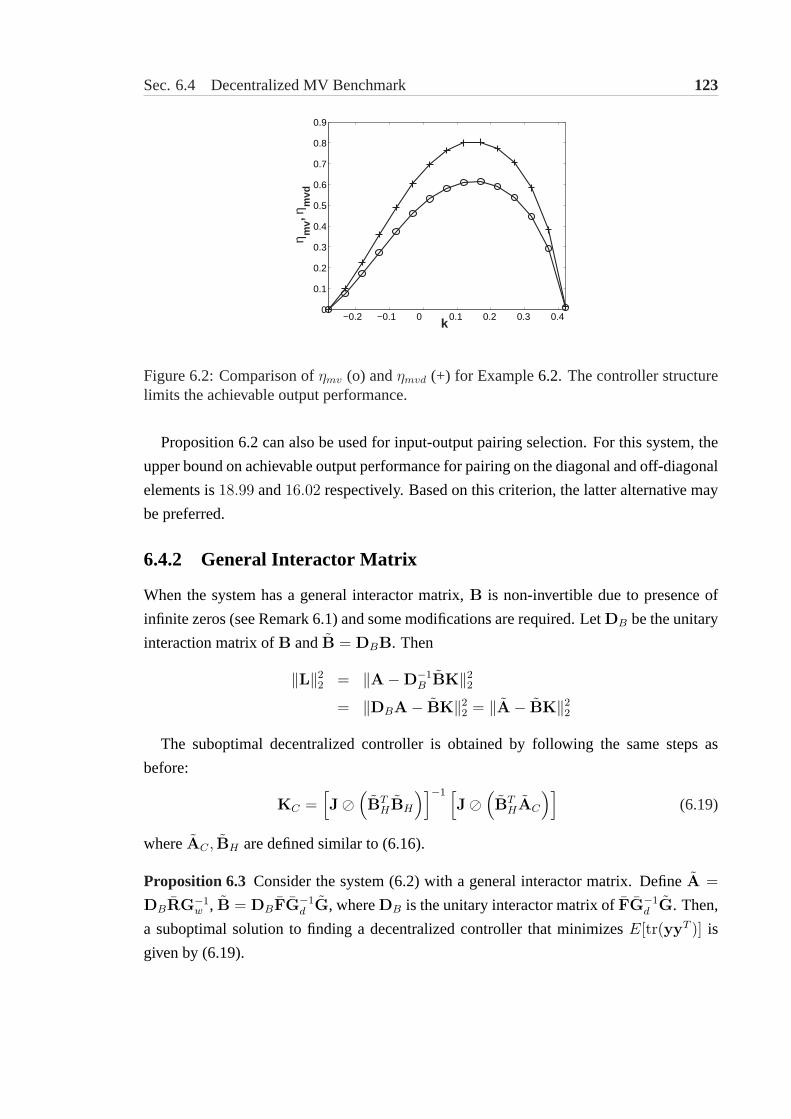
Sec. 6.4 Decentralized MV Benchmark 123
−0.2 −0.1 0 0.1 0.2 0.3 0.4 0
0.1
0.2
0.3
0.4
0.5
0.6
0.7
0.8
0.9
k
η mv, η
mvd
Figure 6.2:Comparison ofηmv (o) andηmvd (+) for Example6.2. The controller structurelimits the achievable output performance.
Proposition6.2can also be used for input-output pairing selection. For this system, the
upper bound on achievable output performance for pairing on the diagonal and off-diagonal
elements is18.99 and16.02 respectively. Based on this criterion, the latter alternative may
be preferred.
6.4.2 General Interactor Matrix
When the system has a general interactor matrix,B is non-invertible due to presence of
infinite zeros (see Remark6.1) and some modifications are required. LetDB be the unitary
interaction matrix ofB andB = DBB. Then
‖L‖22 = ‖A−D−1
B BK‖22
= ‖DBA− BK‖22 = ‖A− BK‖2
2
The suboptimal decentralized controller is obtained by following the same steps as
before:
KC =[J®
(BT
HBH
)]−1 [J®
(BT
HAC
)](6.19)
whereAC , BH are defined similar to (6.16).
Proposition 6.3 Consider the system (6.2) with a general interactor matrix. DefineA =
DBRG−1w , B = DBFG−1
d G, whereDB is the unitary interactor matrix ofFG−1d G. Then,
a suboptimal solution to finding a decentralized controller that minimizesE[tr(yyT )] is
given by (6.19).

124 Chap. 6 Decentralized Minimum Variance Benchmark
0 1 2 3 4 5 6 7 8 9 100.1
0.2
0.3
0.4
0.5
0.6
0.7
0.8
0.9
1
1.1
K12
η mvd
,ηm
v
Figure 6.3:Comparison ofηmv (o) andηmvd (+) for Example6.3. The controller structureposes no serious limitations.
In the previous example, controller structure posed significant limitations on the
achievable performance. This is not always the case, as shown below:
Example 6.3 Consider the following system adapted from Huang and Shah [69],
G =
q−1
1−0.4q−1K12q
−2
1−0.1q−1
0.3q−1
1−0.1q−1q−2
1−0.8q−1
Gw =
11−0.5q−1
−0.61−0.5q−1
0.51−0.5q−1
11−0.5q−1
where the variableK12 controls the extent of interaction among the variables. The objective
is to compare the performance of the following controller for different values ofK12.
K =
[0.5−0.2q−1
1−0.5q−1 0
0 0.25−0.2q−1
(1−0.5q−1)(1+0.5q−1)
]
The ηmvd, ηmv for variousK12 are shown in Figure6.3. For each value ofK12, there
exists a decentralized controller that closely matches the performance of the optimal full
multivariable controller. Hence, the controller structure poses no serious limitation on
the achievable performance for this system. This further illustrates that large interactions
do not necessarily limit the performance of decentralized controllers compared to the full
multivariable controllers.
6.5 Achievable PID Performance
The suboptimal decentralized controller is expressed in terms of its impulse response
matrices. By restricting the order of the controller or settingKk = 0 for all k > p,

Sec. 6.6 Limitations 125
controllers with reduced complexity can be obtained. In this section, this approach is used
to find an overestimate on achievable output variance using multi-loop PID controllers,
which are expressed as,
KPID =1
∆
2∑i=0
Ciq−i =
1
∆C
where∆ = 1 − q−1. By considering1/∆ as a part ofG and minimizing‖L‖22 wrt C,
an overestimate of the achievable PID performance can be derived. Then Propositions6.2
and6.3 can be used by limiting the column dimensions ofAC,BH to 3n. To ensure that
the assumption of stability ofG is satisfied, the integrator can be moved just inside the
unit circle without affecting the result significantly. In general, controllers with reduced
complexity having orderp can be obtained by limiting the column dimensions ofAC,BH
to pn.
Example 6.4 Consider the following system taken from Ko and Edgar [75],
y =q−6
1− 0.8q−1u +
1− 0.2q−1
(1− 0.3q−1)(1 + 0.4q−1)(1− 0.5q−1)a
Clearly the results presented earlier also hold for SISO systems. Based on these results,
the achievable output variances under MV and PI control are1.11 showing that the control
structure poses no limitations. However, when the disturbance model contains an additional
integrator, the achievable output variances under MV and PI control are11.95 and17.86
respectively. The achievable performances differ by more than50% revealing the effect
of controller structure on achievable performance. Note that for both these cases, the
achievable PI performance is close to the results obtained by Ko and Edgar [75], who
used numerical search.
6.6 Limitations
The results presented in this paper require that the system’s model be fully known. This can
be very demanding for online performance monitoring of industrial systems, especially in
presence of changing operating conditions. The requirement of knowledge of the system’s
model can be partially relaxed by estimatingGw using regular operating data, as suggested
by Ko and Edgar [75]. Example6.3 shows that the controller structure does not always
limit the achievable performance. The identification ofG should only be undertaken if
large differences are seen between the actual output variance and MV benchmark for full
multivariable controllers.

126 Chap. 6 Decentralized Minimum Variance Benchmark
The suboptimal controller is expressed in terms of its impulse response matrices, whose
determination is computationally inexpensive. Starting from a low value, the controller
order can be gradually increased until convergence, but convergence can be extremely
slow in some cases. This difficulty is overcome by recognizing that[J® (
BTHBH
)]is
a sparse Toeplitz matrix and using available computationally efficient methods (e.g., Brent
et al. [16]) for its inversion.
The decentralized MV control law is based on an approximation of the closed loop
expression and thus stability is not guaranteed. A possible approach to overcome this
limitation is to reduce the gain of the decentralized controller until stability is achieved,
however, such an approach increases the sub-optimality of the results.
6.7 Chapter Summary
For performance assessment purposes, ignoring the controller structure can lead to
incorrect conclusions regarding significant performance improvement through controller
tuning. In this chapter, we presented an approximate solution to the decentralized minimum
variance control problem, which provides an overestimate of the achievable output variance
without numerical search. The proposed method can easily handle the case of multi-loop
PID controllers. The primary limitation of the proposed method is that complete knowledge
of the system’s model is required and some recommendations are provided to partially
overcome this limitation.

Chapter 7
Conclusions and Future Work
7.1 Thesis Conclusions
In this thesis, we developed tools for handling different aspects of the control configuration
design (CCD) problem. The major contributions are listed below:
• The achievable input performance is characterized for FDLTI systems possibly
having time delay in theH2 andH∞ optimal control frameworks.
• A method for finding a stabilizing decentralized controller through independent
designs is presented. This method extends the practical applicability of theµ-
interaction measure to unstable systems.
• The problem of finding an optimal block diagonal approximation of a multivariate
system is introduced and a numerical solution is proposed.
• Many new algebraic properties of block relative gain (BRG) are developed. The
connection between BRG and important closed loop properties is explored and some
common conjectures are corrected.
• The problem of establishing existence of diagonal controller such that the system has
integrity against controller failure is shown to be NP-hard.
• A suboptimal, yet explicit solution to the decentralized minimum variance
benchmark problem is proposed.
In many cases, the CCD problem can be reasonably solved using the tools presented
in this thesis alone or with possible minor extensions. For example, reliable decentralized
controller can be designed for open loop stable systems using the results of Chapters4- 5.
127

128 Chap. 7 Conclusions and Future Work
In the context of the CCD problem, the results on Decentralized MV benchmark are useful
for screening of pairing alternatives with achievable output performance as a criterion.
We have not handled the important issue of model uncertainty explicitly. Note that
minimization of input energy required for stabilization provides the maximally robust
controller for norm bounded additive uncertainty [43]. The results of Chapter3 can also
be easily extended for handling robust stability and performance issues using the approach
available in [101]. It must be acknowledged; however, that solving the CCD or control
structure design problem for general time-varying non-linear systems remains an open
challenge and this thesis can be seen as a positive step in that direction.
7.2 Directions for Future Work
We pointed out some potential directions for generalizing and improving upon the results
presented in this thesis in the summaries of the individual chapters. Some other relevant
issues are discussed below with the hope that solving these problems will move us closer
towards finding a general solution for the CSD problem.
• The characterization of achievable performance has received increasing interest from
researchers, but the effect of controller structure on the achievable performance
remains unclear. The results of Zames and Bensoussan [116] can be seen as a good
starting point in this direction.
• It is likely that the optimal solution to the block diagonal approximation problem is
not unique. An analytical solution is necessary to characterize all possible solutions.
To this end, it is useful to approach theH∞ optimal block diagonal approximation
problem for stable systems using the results of Gloveret al. [44].
• In some cases, it may not be possible to find a stabilizing decentralized controller
through independent designs. This difficulty can be partially overcome by extending
the ideas presented in Chapter3 for sequential design of decentralized controller for
unstable systems.
• The requirement that a model be available hinders the online implementation of the
decentralized minimum variance benchmark. It would be extremely useful, if exact
or approximate methods can be derived, where this stringent requirement can be
relaxed.

Sec. 7.2 Directions for Future Work 129
• There are no practical tools available (other than numerical simulation) for directly
handling the non-linear behavior of the process systems. An indirect approach
is to approximate the system as a nominal model with an associated uncertainty
description [11], but the involved computational complexity is limiting.


Bibliography
[1] I. M. Alatiqi and W. L. Luyben. Control of a complex sidestream column/stripper
distillation configuration.Ind. Eng. Chem. Process Des. Dev., 25(3):762–767, 1986.
[2] A. E. Andrews.Encyclopedia of Mathematics and its Applications: The Theory of
Partitions. Addison-Wesley Publishing Company, Workingham, UK, 1976.
[3] Y. Arkun. Dynamic block relative gain and its connection with the performance and
stability of decentralized control structures.Intl. J. of Control, 46(4):1187–1193,
1987.
[4] Y. Arkun and J. Downs. A general method to calculate input-output gains and the
relative gain array for integrating processes.Computers Chem. Engng., 14(10):
1101–1110, 1990.
[5] K. J. Astrom. Introduction to Stochastic Control Theory. Academic Press, London,
1970.
[6] J. A. Ball, I. Gohberg, and L. Rodman.Interpolation of Rational Matrix Functions.
Operator Theory: Advances and Applications. Birkhauser Verlag, Basel, Germany,
1990.
[7] J. Bao, J. F. Forbes, and P. J. McLellan. Robust multiloop PID controller design:
A successive semidefinite programming approach.Ind. Eng. Chem. Res., 38:3407–
3419, 1999.
[8] H. W. Bode. Network Analysis and Feedback Amplifier Design. Van Nostrand,
Princeton, NJ, 1945.
[9] S. Boyd and C. Barratt.Linear Controller Design - Limits of Performance. Prentice
Hall, 1991. Available athttp://www.stanford.edu/ ∼boyd/lcdbook/
lcdbook.html .
131
132 Bibliography
[10] S. Boyd, L. E. Ghaoui, E. Feron, and V. Balakrishnan.Linear Matrix Inequalities in
System and Control Theory. SIAM, Philadelphia, 1994.
[11] R. D. Braatz. Robust loopshaping for Process Control. Ph.d., California School
of Technology, Pasadena, CA, May 1993. Available athttp://www.cds.
caltech.edu/reports/index.cgi?year=1993 .
[12] R. D. Braatz, J. H. Lee, and M. Morari. Screening plant designs and control
structures for uncertain systems.Computers Chem. Engg., 20:463–468, 1996.
[13] R. D. Braatz, M. Morari, and S. Skogestad. Robust reliable decentralized control.
In American Control Conference, volume 3, pages 3384–3388, Baltimore, MD, July
1994.
[14] R. D. Braatz and E. L. Russell. Robustness margin computation for large scale
systems.Computers Chem. Engg., 23:1021–1030, 1999.
[15] R. D. Braatz, P. M. Young, J. C. Doyle, and M. Morari. Computational complexity
of µ calculation.IEEE Trans. Automat. Contr., 39(5):1000–1002, 1994.
[16] R. P. Brent, F. G. Gustavson, and D. Y. Yun. Fast solution of Toeplitz systems
of equations and computation of Pade approximants.J. of Algorithms, 1:259–295,
1980.
[17] E. H. Bristol. On a new measure of interaction for multivariable process control.
IEEE Trans. Automat. Contr., 11:133–134, 1966.
[18] P. J. Campo and M. Morari. Achievable closed loop properties of systems under
decentralized control: Conditions involving the steady state gain.IEEE Trans.
Automat. Contr., 39(5):932–943, 1994.
[19] J. J. Castro and F. J. Doyle. Plantwide control of the fiber line in a pulp mill.Ind.
Eng. Chem. Res., 41:1310–1320, 2002.
[20] J. Chen. Relations between block relative gain and Euclidean condition number.
IEEE Trans. Automat. Contr., 37(1):127–129, 1992.
[21] J. Chen. Sensitivity integral relations and design tradeoffs in linear multivariable
feedback control.IEEE Trans. Automat. Contr., 40(10):1700–1716, 1995.

Bibliography 133
[22] J. Chen. Logarithmic integrals, interpolation bounds and performance limitations in
MIMO feedback systems.IEEE Trans. Automat. Contr., 45(6):1098–1115, 2000.
[23] J. Chen, J. S. Freudenberg, and C. N. Nett. The role of the condition number and the
relative gain array in robustness analysis.Automatica, 30(6):1029–1035, 1994.
[24] J. Chen and G. Gu.Control-Oriented System Identification: AnH∞ Approach. John
Wiley & Sons, Mississauga, ON, Canada, 2000.
[25] J. Chen, G. Gu, and C. N. Nett. Worst case identification of continuous time systems
via interpolation.Automatica, 30(12):1825–1837, 1994.
[26] J. Chen, S. Hara, and G. Chen. Best tracking and regulation performance under
control effort constraint: Two parameter controller case.IEEE Trans. Automat.
Contr., 48(8), 2003.
[27] J. Chen and R. H. Middleton. New development and applications in performance
limitations of feedback systems.IEEE Trans. Automat. Contr., 48(8), 2003.
[28] M. Chilai and P. Gahinet.H∞ design with pole placement constraints: An LMI
approach.IEEE Trans. Automat. Contr., 41(3):358–367, 1993.
[29] C. S. Chin and N. Munro. The analysis and control of the ALSTOM gasifier
benchmark problem.Proceedings of XV IFAC World Congress, Barcelona, Spain,
2002.
[30] M. S. Chiu and Y. Arkun. Decentralized control structure selection based on integrity
considerations.Ind. Eng. Chem. Res., 29(3):369–373, 1990.
[31] G. E. Coxson. The P-matrix problem is co-NP-complete.Mathematical
Programming, 64:173–178, 1994.
[32] R. Dixon, A. W. Pike, and M. S. Donne. The ALSTOM benchmark challenge on
gasifier control.Proc. Instn. Mech. Engrs, Part I, Journal of Systems and Control
Engineering, 214(16):389–394, 2000.
[33] J. J. Downs and E. F. Vogel. A plant-wide industrial process control problem.
Computers Chem. Engng., 17:245–255, 1993.

134 Bibliography
[34] J. C. Doyle, K. Glover, P. Khargonekar, and B. Francis. State-space solutions to
standardH2 andH∞ control problems.IEEE Trans. Automat. Contr., 34(8):831–
847, 1989.
[35] J. C. Doyle, J. E. Wall, and G. Stein. Performance and robustness analysis for
structured uncertainty.Proceedings of IEEE Conf. on Decision and Control, 1982.
[36] A. S. Foss. Critique of chemical process control theory.AICHE J., 19(2):209–214,
1973.
[37] B. A. Francis.A Course inH∞ Control Theory. Springer-Verlag, New York, 1987.
[38] J. S. Freudenberg and D. P. Looze. Right half plane zeros and poles and design
tradeoffs in feedback systems.IEEE Trans. Automat. Contr., 30:555–565, June 1985.
[39] M. Fu. The real structured singular value is hardly approximable.IEEE Trans.
Automat. Contr., 42(9):1286–1288, 1997.
[40] C. E. Garcia and M. Morari. Internal model control 2. Design procedure for
multivariate systems.Ind. Eng. Chem. Process Des. Dev., 24(2):472–484, 1985.
[41] M. R. Garey and D. S. Johnson.Computers and Intractability: A guide to NP-
completeness. W. H. Freeman and Company, New York, 1983.
[42] K. Glover. All optimal hankel-norm approximations of linear multivariable systems
and theirL∞ bounds.Int. J. of Control, 39(6):1115–1193, 1984.
[43] K. Glover. Robust stabilization of linear multivariable systems: Relations to
approximation.Int. J. of Control, 43(3):741–766, 1986.
[44] K. Glover, D. J. N. Limbeer, and Y. S. Hung. A structured approximation problem
with applications to weighted model reduction.IEEE Trans. Automat. Contr., 37(4):
447–465, 1992.
[45] G. C. Goodwin and K. Sin.Adaptive Filtering Prediction and Control. Prentice-
Hall, Englewood Cliffs, 1984.
[46] M. S. Govatsmark.Integrated Optimization and Control. PhD thesis, Norwegian
Institute of Science and Technology, Trondheim, Norway, September 2003.
[47] M. Green and D. J. N. Limebeer.Linear Robust Control. Prentice-Hall, New Jersey,
1995.

Bibliography 135
[48] P. Grosdidier. Analysis of interaction direction with the singular value
decomposition.Computers Chem. Engng., 14(6):687–689, 1990.
[49] P. Grosdidier and M. Morari. Interaction measures for systems under decentralized
control. Automatica, 22(3):309–319, 1986.
[50] P. Grosdidier and M. Morari. A computer aided methodology for the design of
decentralized controllers.Comput. Chem. Engng., 11(4):423–433, 1987.
[51] P. Grosdidier, M. Morari, and B. R. Holt. Closed-loop properties from steady-state
gain information.Ind. Eng. Chem. Fundam., 24:221–235, 1985.
[52] A. N. Gundes and M. G. Kabuli. Reliable decentralized-integral action controller
design.IEEE Trans. Automat. Contr., 46(2):296–301, 2001.
[53] T. J. Harris. Assessment of control loop performance.Can. J. of Chem. Engng., 67:
856–861, 1989.
[54] T. J. Harris, F. Boudreau, and J. F. Macgregor. Performance assessment of
multivariable feedback controllers.Automatica, 32(11):1505–1518, 1996.
[55] T. J. Harris, C. T. Seppala, and L. D. Desborough. A review of performance
monitoring and assessment techniques for univariate and multivariate control
systems.J. Proc. Control, 9:1–17, 1999.
[56] K. Havre. Studies on Controllability analysis and Control Structure Design. PhD
thesis, Norwegian University of Science and Technology, Trondheim, Norway,
January 1998. Available athttp://www.nt.ntnu.no/users/skoge/
publications/thesis/1998/havre/ .
[57] K. Havre and S. Skogestad. Achievable performance of multivariable systems with
unstable zeros and poles.Intl. J. of Control, 74:1131–1139, 2001.
[58] K. Havre and S. Skogestad. Selection of variables for stabilizing control using pole
vectors.IEEE Trans. Automat. Contr., 48(8):1393–1398, 2003.
[59] K. E. Haggblom. Partial relative gain: A new tool for control structure selection,
1997. Presented at AICHE annual meeting, Los Angeles, Available athttp:
//www.abo.fi/fak/ktf/rt/papers/aic97kh1.pdf .

136 Bibliography
[60] A. J. Helmicki, C. A. Jacobson, and C. N. Nett. Control oriented system
identification: A worst-case/deterministic approach inH∞. IEEE Trans. Automat.
Contr., 36(10):1163–1176, 1991.
[61] A. J. Helmicki, C. A. Jacobson, and C. N. Nett. Worst-case/deterministic approach
in H∞: The continuous-time case.IEEE Trans. Automat. Contr., 37(5):604–610,
1992.
[62] R. A. Horn and C. R. Johnson.Matrix Analysis. Cambridge University Press,
Cambridge, UK, 1985.
[63] R. A. Horn and C. R. Johnson.Topics in Matrix Analysis. Cambridge University
Press, Cambridge, UK, 1991.
[64] M. Hovd, D. L. Ma, and R. D. Braatz. On the computation of disturbance rejection
measures.Ind. Eng. Chem. Res., 42:2183–2188, 2003.
[65] M. Hovd and S. Skogestad. Simple frequency dependent tools for control system
analysis.Automatica, 28:989–996, 1992.
[66] M. Hovd and S. Skogestad. Improved independent design of robust decentralized
controllers.J. Process Control, 3:43–51, 1993.
[67] M. Hovd and S. Skogestad. Sequential design of decentralized controllers.
Automatica, 30(10):1601–1607, 1994.
[68] B. Huang and S. L. Shah. The role of the unitary interactor matrix in the explicit
solution of the singular LQ output feedback control problem.Automatica, 33(11):
2071–2075, 1997.
[69] B. Huang and S. L. Shah.Performance Assessment of Control Loops: Theory and
Applications. Springer-Verlag, London, 1999.
[70] B. Huang, S. L. Shah, and E. K. Kwok. Good, bad or optimal? Performance
assessment of multivariate processes.Automatica, 33(6):1175–1183, 1997.
[71] C. R. Johnson and H. M. Shapiro. Mathematical aspects of the relative gain array
(A ◦ A−T). SIAM J. Alg. Dis. Meth., 7(4):627–644, 1986.
[72] V. Kariwala, J. F. Forbes, and E. S. Meadows. Block relative gain: Properties and
pairing rules.Ind. Eng. Chem. Res., 42(20):4564–4574, 2003.

Bibliography 137
[73] V. Kariwala, J. F. Forbes, and E. S. Meadows. Closed loop properties and block
relative gain. In7th International Symposium on Advanced Control of Chemical
Processes, Hong Kong, P.R. China, January 2004. Available athttp://www.
ualberta.ca/dept/chemeng/control/reports.html .
[74] V. Kariwala, S. Skogestad, J. F. Forbes, and E. S. Meadows. Input performance
limitations of feedback control. InAmerican Control Conference, Boston,
MA, July 2004. Available athttp://www.ualberta.ca/dept/chemeng/
control/reports.html .
[75] B. Ko and T. F. Edgar. Assessment of acheivable PI performance for linear processes
with dead time. InAmerican Control Conference, Philadelphia, PA, 1998.
[76] H. Kwaakernaak and R. Sivan.Linear Optimal Control Systems. John Wiley &
Sons, Inc., New York, 1972.
[77] L. Li and K. Zhou. An approximation approach to decentralizedH∞ control.
In Proceedings of4th World Congress on Intelligent Control and Automation,
Shanghai, China, June 2002.
[78] D. J. N. Limbeer. The application of generalized diagonal dominance to linear
system stability theory.Int. J. of Control, 36(2):185–212, 1982.
[79] W. L. Luyben, B. Tyreus, and M. L. Luyben.Plantwide Process Control. McGraw-
Hill, 1998.
[80] D. L. Ma, J. G. VanAntwerp, M. Hovd, and R. D. Braatz. Quantifying the potential
benefits of constrained control for a large scale system.IEE Proceedings - Control
Theory and Application, 149:423–432, 2002.
[81] A. G. J. MacFarlane and N. Karcanias. Poles and zeros of linear multivariable
systems: A survey of algebraic, geometric and complex variable theory.Intl. J.
Control, 24:33–74, 1976.
[82] V. Manousiouthakis and M. Nikolaou. Analysis of decentralized control structures
for non-linear systems.AIChE J., 35(4):549–558, 1989.
[83] V. Manousiouthakis, R. Savage, and Y. Arkun. Synthesis of decentralized process
control structures using the concept of block relative gain.AIChE J., 32(6):991–
1003, 1986.

138 Bibliography
[84] D. Q. Mayne. The design of linear multivariable systems.Automatica, 9(3):201–
207, 1973.
[85] C. N. Nett and V. Manousiouthakis. Euclidean condition and block relative gain:
Connections, conjectures and clarifications.IEEE Trans. Automat. Contr., 32(5):
405–407, 1987.
[86] C. N. Nett and K. D. Minto. A quantitative approach for selection and partitioning
of measurements and manipulations for control of complex systems, June 1989.
Presented atAmerican Control Conference, Pittsburgh, Pennsylvania.
[87] A. Niederlinski. A heuristic approach to the design of linear multivariate interacting
control systems.Automatica, 7:691–701, 1971.
[88] Y. Ohta, D. D. Siljek, and T. Matsumoto. Decentralized control using quasi-block
diagonal dominance of transfer function matrices.IEEE Trans. Automat. Contr., 31
(5):420–429, 1986.
[89] Y. Peng and M. Kinnaert. Explicit solution to the singular LQ regulation problem.
IEEE Trans. Automat. Contr., 37(5):633–636, 1992.
[90] R. Pintleton, P. Guillaume, Y. Rolaine, J. Shouckens, and H. Van hamme. Parametric
identification of transfer functions in the frequency domain - A survey.IEEE Trans.
Automat. Contr., 39(11):2245–2260, 1994.
[91] S. J. Qin. Controller performance monitoring - A review and assessment.Computers
Chem. Engng., 23:173–186, 1998.
[92] L. Qiu and E. J. Davison. Performance limitations of non-minimum phase systems
in the servomechanism problem.Automatica, 29(2):337–349, 1993.
[93] D. E. Reeves and Y. Arkun. Interaction measures for nonsquare decentralized control
structures.AICHE J., 35(4):603–613, 1989.
[94] H. H. Rosenbrock.Computer-Aided Control System Design. Academic Press, New
York, 1974.
[95] S. M. Rump. On P-matrices.Linear Algebra and Applications, 363:237–250, 2003.
[96] Y. Samyudia, P. L. Lee, and I. T. Cameron. A new approach to decentralized control
design.Chem. Eng. Sci., 50(11):1695–1706, 1995.

Bibliography 139
[97] M. M. Seron, J. H. Braslavsky, and G. C. Goodwin.Fundamental Limitations in
Filtering and Control. Springer-Verlag, London, 1997.
[98] D. D. Siljek. Decentralized control and computations: Status and prospects.A. Rev.
Control, 20:131–141, 1996.
[99] S. Skogestad. Plantwide control: The search for the self-optimizing control
structure.J. Proc. Control, 10:487–507, 2000.
[100] S. Skogestad and M. Morari. Some new properties of the structured singular value.
IEEE Trans. Automat. Contr., 33(12):1151–1154, 1988.
[101] S. Skogestad and M. Morari. Robust performance of decentralized control systems
by independent designs.Automatica, 25(1):119–125, 1989.
[102] S. Skogestad and I. Postlethwaite.Multivariable Feedback Control: Analysis and
design. John Wiley & Sons, Chichester, UK, 1996.
[103] D. D. Sourlas and V. Manousiouthakis. Best achievable decentralized performance.
IEEE Trans. Automat. Contr., 40(11):1858–1871, 1995.
[104] G. Stein. Respect the unstable.IEEE Control systems Magazine, 23(4):12–15,
20003.
[105] M. J. Tsatsomeros and L. Li. A recursive test for P-matrices.BIT, 40(2):410–414,
2000.
[106] M. Van de wal. Control structure design for dynamic systems: A review.
Technical Report WFW-94-084, Eindhoven University of Technology, Eidnhoven,
Netherlands, September 1994.
[107] M. Van de Wal and B. de Jager. A review of methods for input/output selection.
Automatica, 37:487–510, 2001.
[108] J. G. VanAntwerp and R. D. Braatz. A tutorial on linear and bilinear matrix
inequalities.J. Proc. Contr., 10:363–385, 2000.
[109] M. Vidyasagar. Control Systems Synthesis: A Factorization Approach. Series in
signal processing, optimization and control. MIT Press, Cambridge, MA, 1985.
[110] G. Vinnicombe.Uncertainty and Feedback. World Scientific, London, 1999.

140 Bibliography
[111] J. E. Wall, J. C. Doyle, and C. A. Harvey. Tradeoffs in design of multivariate
feedback systems. InProceedings of18th Annual Allerton Conf. on Communication,
Control and Computing, pages 725–735, October 1980.
[112] S. Wang and E. J. Davison. On the stabilization of decentralized control systems.
IEEE Trans. Automat. Contr., 18(5):473–478, 1973.
[113] C. C. Yu and W. L. Luyben. Robustness with respect to integral contrallability.Ind.
Eng. Chem. Res., 26:1043–1045, 1987.
[114] J. I. Yuz and G. C. Goodwin. Loop performance assessment for decentralized control
of stable linear systems.European J. of Control, 9:116–130, 2003.
[115] G. Zames. Feedback and optimal sensitivity: Model reference transformations,
multiplicative seminorms, and approximate inverses.IEEE Trans. Automat. Contr.,
26(2):301–320, 1981.
[116] G. Zames and D. Bensoussan. Multivariable feedback, sensitivity, and decentralized
control. IEEE Trans. Automat. Contr., 28(11):1030–1035, 1983.
[117] K. Zhou and J. C. Doyle.Essentials of Robust Control. Prentice Hall, New Jersey,
1998.