© The McGraw-Hill Companies, 2005 CONSUMPTION, TIME ALLOCATION, AND PRODUCTION CHOICES

©The McGraw-Hill Companies, 2005

CONSUMPTION, TIME ALLOCATION, AND PRODUCTION CHOICES


Themes of the chapter

Why study consumption?

The simple Keynesian consumption function

The consumer’s intertemporal budget constraint

Optimal allocation of consumption over time

The relationship between consumption, income, interest and wealth

Taxation, public debt and private consumption


THREE GOOD REASONS FOR STUDYING PRIVATE CONSUMPTION

Private consumption is by far the largest component of aggregate demand

Economic welfare depends in large part on consumption

The counterpart to consumption is saving which is a precondition for capital formation and long run growth


Focus of the chapter

Focus on total consumption

Focus on the allocation of consumption over time


THE SIMPLE KEYNESIAN CONSUMPTION FUNCTION

, 0, 0 1dt tC a b Y a b

b = dC/dYd = marginal propensity to consume

C/Yd = b+a/Yd = average propensity to consume

(1)


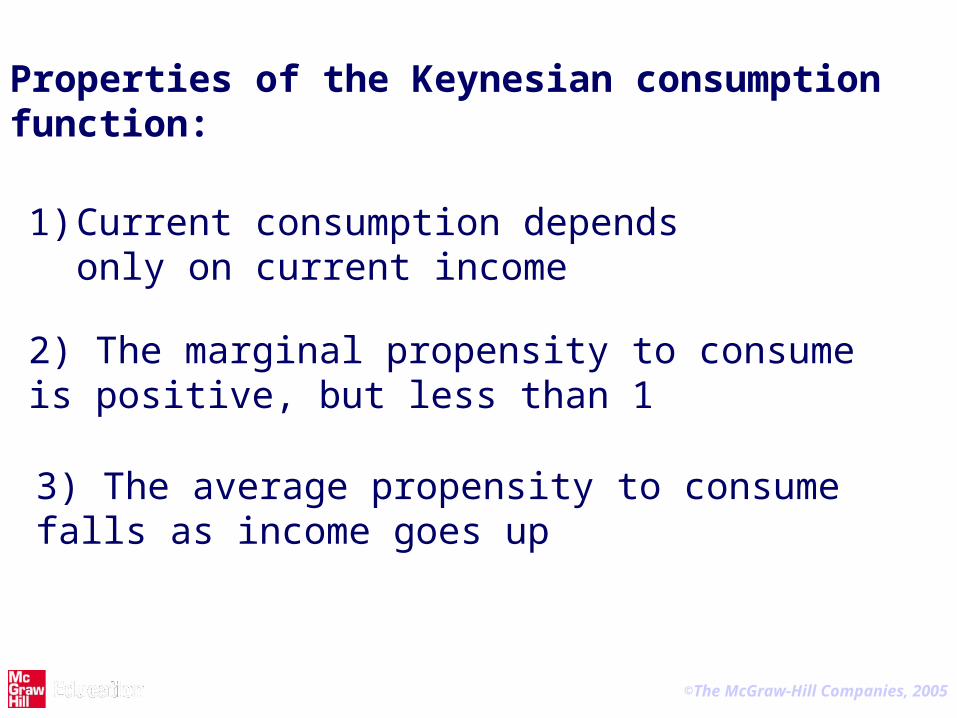
1) Current consumption depends only on current income

2) The marginal propensity to consume is positive, but less than 1

3) The average propensity to consume falls as income goes up

Properties of the Keynesian consumption function:


PROBLEMS WITH THEKEYNESIAN CONSUMPTION FUNCTION

Theoretical problem: Why should consumption depend only on current income?

Empirical problem: Microeconomic cross section data suggest that the average propensity to consume falls as income goes up

but

Macroeconomic time series data show that the average propensity to consume does not systematically fall with rising income, but that it isroughly constant


Consumption

Disposable income

45o

Consumption

Consumption

Disposable income

45o

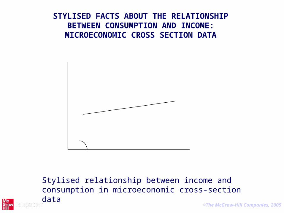
STYLISED FACTS ABOUT THE RELATIONSHIPBETWEEN CONSUMPTION AND INCOME:MICROECONOMIC CROSS SECTION DATA

Stylised relationship between income and consumption in microeconomic cross-section data


45o

Consumption

Disposable income

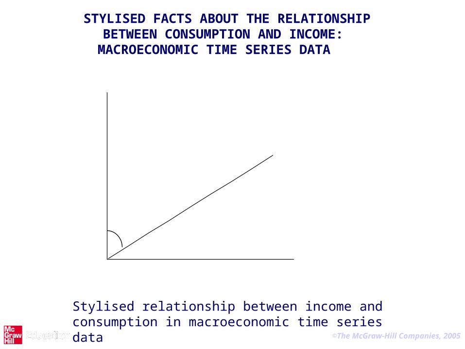
STYLISED FACTS ABOUT THE RELATIONSHIPBETWEEN CONSUMPTION AND INCOME:

MACROECONOMIC TIME SERIES DATA

45o

Consumption

Consumption

Disposable income

Stylised relationship between income and consumption in macroeconomic time series data


0

0.2

0.4

0.6

0.8

1

1.2

1929 1933 1937 1941 1945 1949 1953 1957 1961 1965 1969 1973 1977 1981 1985 1989 1993 1997 2001

Year

Aggregate consumption / aggregate disposable household income

0

0.2

0.4

0.6

0.8

1

1.2

1929 1933 1937 1941 1945 1949 1953 1957 1961 1965 1969 1973 1977 1981 1985 1989 1993 1997 2001

USA

Year


0

0.2

0.4

0.6

0.8

1

1.2

1929 1933 1937 1941 1945 1949 1953 1957 1961 1965 1969 1973 1977 1981 1985 1989 1993 1997 2001

USA

Denmark

Year


THE EVOLUTION OF THE AVERAGE PROPENSITY TO CONSUME IN THE UNITED STATES AND DENMARK

The average propensity to consume in USA and Denmark


CRITERIA FOR A SATISFACTORYTHEORY OF CONSUMPTION

The theory must be consistent with optimizing behaviour at the micro level

The theory must be consistent with the microeconomic cross section data as well as with the macroeconomic time series data

In the following we will try to develop such a theory of consumption


CONSUMER PREFERENCES

The representative consumer’s planning horizon is divided into two periods:

‘the present’ (period 1) and ‘the future’ (period 2) Lifetime utility:

21

( )( ) , ' 0, '' 0, 0

1

u CU u C u u

(2)

Properties of the utility function:

the marginal utility of consumption in each period is positive, but diminishing (provides an incentive for consumption smoothing) the consumer is impatient: the rate of time preference is positive


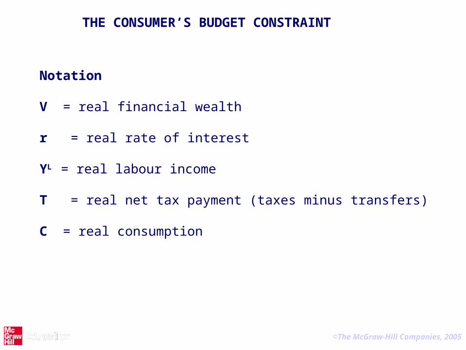
THE CONSUMER’S BUDGET CONSTRAINT

Notation V = real financial wealth r = real rate of interest YL = real labour income T = real net tax payment (taxes minus transfers) C = real consumption



Assumptions

● all payments take place at the start of each period (unimportant assumption)

● the capital market is perfect (no borrowing constraints)

The budget constraint for period 1

2 1 1 1 11 LV r V Y T C (3)

The budget constraint for period 2

2 2 2 2LC V Y T (4)



Insert (3) into (4) to get


2 2 21 1 1 11 1

LLC Y T

C V Y Tr r

(5)

Implication: the present value of total consumption over the life cycle cannot exceed the present value of disposable lifetime income plus the initial stock of wealth



We can simplify the budget constraint by introducing the concept of

Human wealth (human capital) 2 2

1 1 1 1

LL Y T

H Y Tr

(9)

Human wealth is given by the present value of disposable labour income overthe remaining part of the life cycle Substitution of (9) into (8) yields a simplified expression for

The intertemporal budget constraint

21 1 11

CC V H

r

(10)


OPTIMAL ALLOCATION OF CONSUMPTION OVER TIME

Substitution of the budget constraint (10) into the utility function (2) yields

1 1 11

(1 )( )( )

1

u r V H CU u C

(11)

Maximization of (11) with respect to C1 yields the first-order condition

2

1 1 1 11

1 2

10 '( ) ' (1 )( )

1

1 '( ) '( )

1

C

dU ru C u r V H C

dC

ru C u C

(12)

Interpretation: In the optimum the consumer is indifferent between consuming an extra unit today and saving an extra unit today


OPTIMAL ALLOCATION OF CONSUMPTION OVER TIME By rearranging (12) we get

The Keynes-Ramsey rule

1

2

'( )1

'( ) /(1 )

u Cr

u C

(13)

Interpretation: the marginal rate of substitution between present and future consumption (the left-hand side) must equal the relative price of present consumption (the right-hand side), as shown in Figure 16.3.

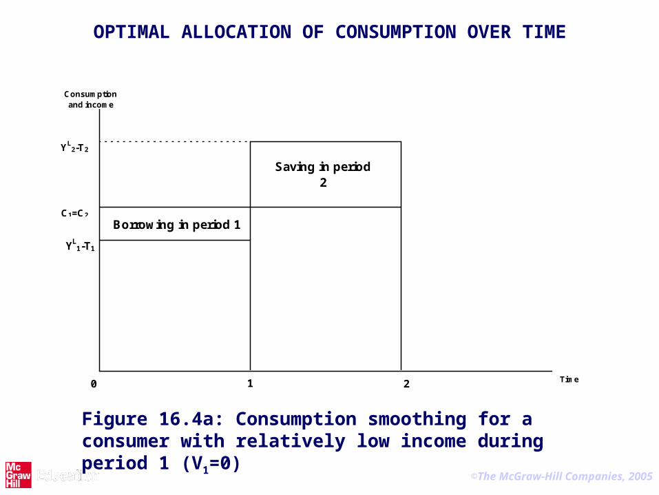
Note: For r= it follows from (12) and (13) that the consumer wishes to smooth consumption completely, that is C1 = C2 . Figure 16.4 illustratesconsumption smoothing in the case where V1 = 0.


C2

C1

|slope| = 1 + r

H1+V1

optimal intertemporal allocation of consumption

C2

C1

|slope| = MRS (C2 : C1 )

|slope| = 1 + r

H1+V1

saving

V1+YL1-T1


Figure 16.3: The consumer’s optimal intertemporal allocation of consumption


Borrowing in period 1

Saving in period 2

Consumption and income

Time1 2

YL2-T2

C1=C2

YL1-T1

0


Figure 16.4a: Consumption smoothing for a consumer with relatively low income during period 1 (V1=0)


OPTIMAL ALLOCATION OF CONSUMPITON OVER TIME

Saving in period 1

Dissaving in period 2

1 20

Consumption and income

Time

YL2-T2

C1=C2

YL1-T1

Figure 16.4b: Consumption smoothing for a consumer with relatively high income during period 1 (V1=0)


DO CONSUMERS ACTUALLY SMOOTH CONSUMPTION?

consumption and income profiles for couples in UK (born 1935-1939)age

income consumption adjusted consumption

30 40 50 60

-2.2

-2

-1.8

-1.6

Figure 16.5: Consumption and income profiles for households in the United Kingdom (born 1935-1939)


DERIVING THE CONSUMPTION FUNCTION

Suppose now that the consumer’s utility function takes the form

1 1/1( ) for 0, 1

1 1/

( ) ln for =1

t t

t t

u C C

u C C

(15.a)

(15.b)

To analyze the properties of this utility function, we introduce the intertemporal elasticity of substitution in consumption (IES), defined as

2 1 2 1 2 1

2 1 2 1 2 1

( / ) /( / ) ln( / )

( : ) / ( : ) ln ( : )

d C C C C d C CIES

dMRS C C MRS C C d MRS C C (16)

IES measures the degree to which the consumer is willing to substitute between current and future consumption, as illustrated in Figure 16.6.


C2

C1

indifference curve

C2

C1

C0

C01

E0

slope=C02/C0

1

|slope|=MRS(C02:C0

1)

indifference curve

Figure 16.6: The relation between the consumption ratio (C2/C1) and the marginal rate of substitution

C2

C1

C1

2

C0

C11 C0

1

E1

E0

slope=C12/C

11

slope=C02/C

01

|slope|=MRS(C12:C

11)

|slope|=MRS(C02:C

01)

indifference curve


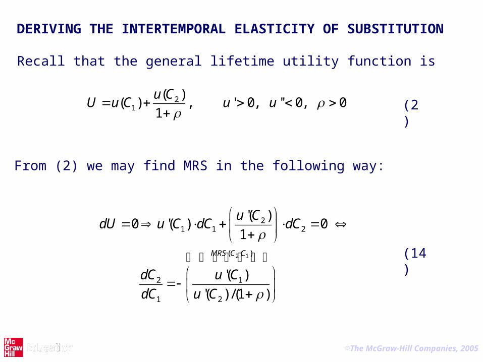
DERIVING THE INTERTEMPORAL ELASTICITY OF SUBSTITUTION Recall that the general lifetime utility function is

21

( )( ) , ' 0, '' 0, 0

1

u CU u C u u

(2)

From (2) we may find MRS in the following way:

2 1

21 1 2

( : )

2 1

1 2

'( )0 '( ) 0

1

'( )

'( ) /(1 )

MRS C C

u CdU u C dC dC

dC u C

dC u C

(14)


According to equation (15.a) we have

which implies that

u’(Ct) = Ct-1/ (15.c)

1 1/1( ) for 0, 1

1 1/t tu C C

DERIVING THE INTERTEMPORAL ELASTICITY OF SUBSTITUTION


DERIVING THE IES

Using (14), (15.c) and the definition of IES given in (16), we now find that

1/1/1 1

2 1 2 11/2 2

2 1 2 1

'( )( : ) (1 )( / )

'( ) /(1 ) /(1 )

ln ( : ) ln(1 ) (1/ ) ln( / )

u C CMRS C C C C

u C C

MRS C C C C

2 1 2 1

2 1 2 1

2 1 2 1

ln ( : ) (1/ ) ln( / )

ln( / ) ln( / )

ln ( : ) (1/ ) ln( / )

d MRS C C d C C

d C C d C CIES

d MRS C C d C C

(17)


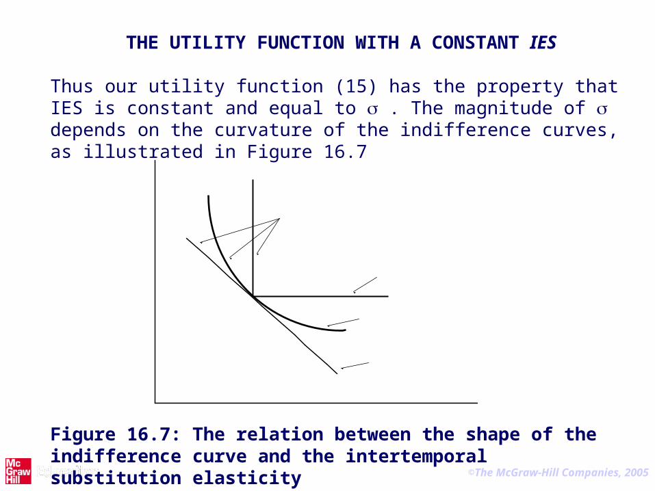
THE UTILITY FUNCTION WITH A CONSTANT IES

Thus our utility function (15) has the property that IES is constant and equal to . The magnitude of depends on the curvature of the indifference curves, as illustrated in Figure 16.7 C2

C1

indifference curves

0 < < ∞

= 0

Figure 16.7: The relation between the shape of the indifference curve and the intertemporal substitution elasticity


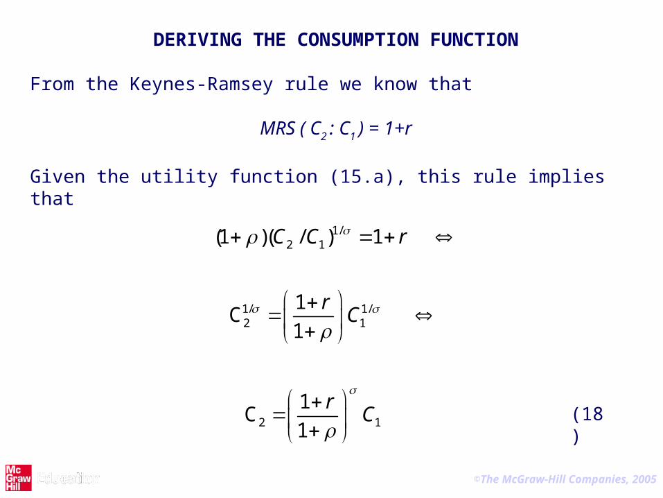
DERIVING THE CONSUMPTION FUNCTION From the Keynes-Ramsey rule we know that

MRS ( C2 : C1 ) = 1+r Given the utility function (15.a), this rule implies that

1/2 1

1/ 1/2 1

2 1

(1 )( / ) 1

1 C

1

1 C

1

C C r

rC

rC

(18)


DERIVING THE CONSUMPTION FUNCTION

From the intertemporal budget constraint (10) we know that

21 1 11

CC V H

r

Inserting (18) into (10), we get

11 1 1 1

1 1 1

1

(1 ) (1 )

( ),

10 1

1 (1 ) (1 )

C r C V H

C V H

r

Implication: Current consumption is proportional to total current wealth.The propensity to consume wealth is positive, but less than one.

(19)

(10)


CONSUMPTION AND INCOME Using the definition of human wealth given in (9), we find from (19) that

21 1 1 ,

1

dd d L

t t t

YC Y V Y Y T

r

(20)

which may be rewritten as

1

1

ˆd

C

Y

2 11 1

1 1

ˆ 1 , , 1

d

d d

R Y Vv R v

r Y Y

(21)

(22)

If the expected rate of income growth is denoted by g, we may write equation (20) in the following way:

11

1

11

1d

C gv

Y r

(23)


EXPLAINING THE RELATIONSHIPBETWEEN CONSUMPTION AND INCOME

Cross section data: In a cross section of consumers in a given year many persons with a low current income may expect to earn a higher future income. Hence they will have a high propensity to consume, since R in (22) will be high. Other individuals with high current incomes will expect a lower future income (a low value of R) and will therefore have a low propensity to consume.

The difference between current and future income may be due to the fact that income varies systematically over the life cycle (the life cycle theory, Modigliani), or may be due to temporary random fluctuations in income (the permanent income theory, Friedman).

Time series data: In the long run the variables g, r and v1 are roughly constant. Hence the average propensity to consume will also be roughly constant, according to (23).


0.8

0.85

0.9

0.95

1

1.05

1.1

1966 1968 1970 1972 1974 1976 1978 1980 1982 1984 1986 1988 1990 1992 1994 1996 1998 2000

4

4.5

5

5.5

6

6.5

Average propensity to

consume1

Wealth-income

ratio2

0.8

0.85

0.9

0.95

1

1.05

1.1

1966 1968 1970 1972 1974 1976 1978 1980 1982 1984 1986 1988 1990 1992 1994 1996 1998 2000

4

4.5

5

5.5

6

6.5

Wealth-income ratio(right axis)


consume1

Wealth-income

ratio2

0.8

0.85

0.9

0.95

1

1.05

1.1

1966 1968 1970 1972 1974 1976 1978 1980 1982 1984 1986 1988 1990 1992 1994 1996 1998 2000

4

4.5

5

5.5

6

6.5


consume(left axis)

Wealth-income ratio(right axis)


consume1

Wealth-income

ratio2

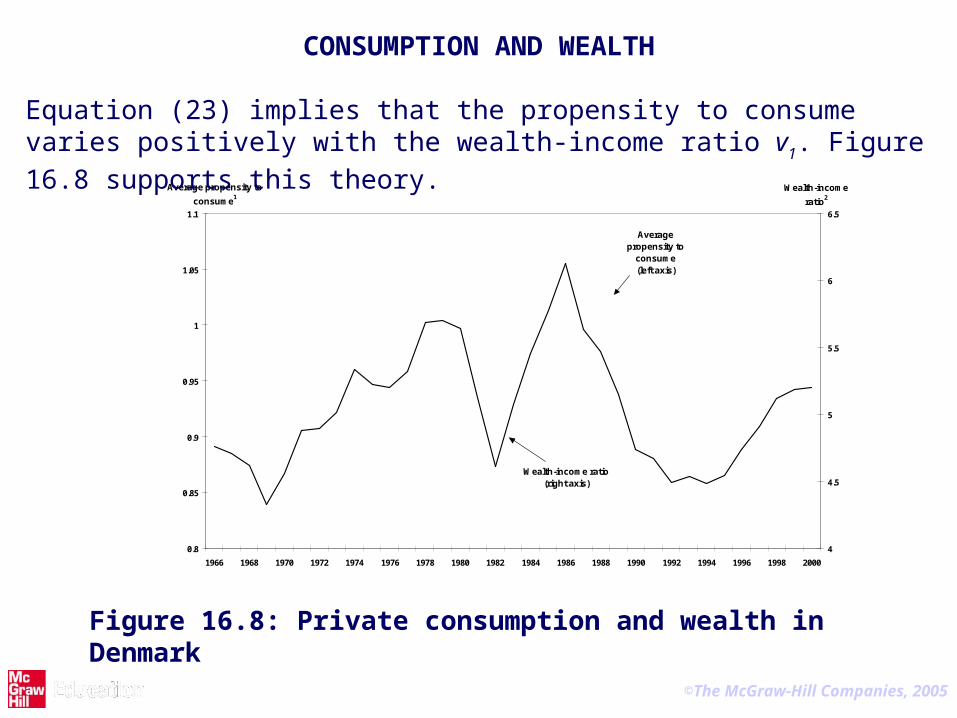
CONSUMPTION AND WEALTH Equation (23) implies that the propensity to consume varies positively with the wealth-income ratio v1. Figure 16.8 supports this theory.

Figure 16.8: Private consumption and wealth in Denmark


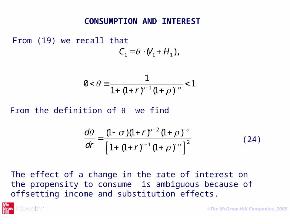
CONSUMPTION AND INTEREST

From (19) we recall that

1 1 1

1

( ),

10 1

1 (1 ) (1 )

C V H

r

From the definition of we find

2

21

(1 )(1 ) (1 )

1 (1 ) (1 )

d r

dr r

The effect of a change in the rate of interest on the propensity to consume is ambiguous because of offsetting income and substitution effects.

(24)


CONSUMPTION AND INTEREST However, a rise in the real rate of interest also has two negative wealth effects on consumption:

The human wealth effect: A rise in the rate of interest reduces the present value of lifetime labour income, since

2 21 1 1 1

LL Y T

H Y Tr

(9)

The financial wealth effect: A rise in the rate of interest reduces the market value of financial wealth, since stock prices and housing prices vary negatively with the real interest rate.


THE GENERALIZED CONSUMPTION FUNCTION

We may summarize our theory of private consumption in the generalised consumption function:

1 1 1(?)( )( ) ( )

, , ,dC C Y g r V

(36)

Expectations about the future affect consumption via g and via V1


IMPORTANT CONCEPTS AND POINTS IN CHAPTER 16

The simple Keynesian consumption function

The lifetime utility function, the rate of time preference and the intertemporal elasticity of substitution


Human capital

The optimal allocation of consumption over time: the Keynes-Ramsey rule and consumption smoothing

Derivation of the consumption function

Explanation of the relationship between income and consumption in cross section data and in time series data: the life cycle theory and the permanent income theory


IMPORTANT CONCEPTS AND POINTS IN CHAPTER 16

The relationship between wealth and consumption

The relationship between the real interest rate and consumption

The effects of temporary and permanent tax cuts

The intertemporal government budget constraint

The Ricardian Equivalence Theorem

Reasons why Ricardian Equivalence is likely to fail

Documents

© The McGraw-Hill Companies, 2005 CONSUMPTION, TIME ALLOCATION, AND PRODUCTION CHOICES