Embed Size (px)
Citation preview

ADAPTIVE NONLINEAR SYSTEM IDENTIFICATION AND CHANNEL EQUALIZATION USING
FUNCTIONAL LINK ARTIFICIAL NEURAL NETWORK
A THESIS SUBMITTED IN PARTIAL FULFILLMENT
OF THE REQUIREMENTS FOR THE DEGREE OF
Master of Technology
in
Telematics and Signal Processing
By
AJIT KUMAR SAHOO
Department of Electronics and Communication Engineering
National Institute Of Technology
Rourkela
2007

ADAPTIVE NONLINEAR SYSTEM IDENTIFICATION AND CHANNEL EQUALIZATION USING
FUNCTIONAL LINK ARTIFICIAL NEURAL NETWORK
A THESIS SUBMITTED IN PARTIAL FULFILLMENT
OF THE REQUIREMENTS FOR THE DEGREE OF
Master of Technology in
Telematics and Signal Processing
By
AJIT KUMAR SAHOO
Under the Guidance of Prof. G. Panda
Department of Electronics and Communication Engineering
National Institute Of Technology
Rourkela
2007

National Institute Of Technology
Rourkela
CERTIFICATE
This is to certify that the thesis entitled, “Adaptive Nonlinear System Identification and
Channel Equalization Using Functional Link Artificial Neural Network” submitted by
Sri Ajit kumar Sahoo in partial fulfillment of the requirements for the award of Master of
Technology Degree in Electronics & communication Engineering with specialization in
“Telematics and Signal Processing” at the National Institute of Technology, Rourkela
(Deemed University) is an authentic work carried out by him under my supervision and
guidance.
To the best of my knowledge, the matter embodied in the thesis has not been submitted to any
other University / Institute for the award of any Degree or Diploma.
Prof. G. Panda Dept. of Electronics & Communication Engg.
Date: National Institute of Technology Rourkela-769008

ACKNOWLEDGEMENTS
This project is by far the most significant accomplishment in my life and it would be
impossible without people who supported me and believed in me.
I would like to extend my gratitude and my sincere thanks to my honorable, esteemed
supervisor Prof. G. Panda, Head, Department of Electronics and Communication
Engineering. He is not only a great lecturer with deep vision but also most importantly a kind
person. I sincerely thank for his exemplary guidance and encouragement. His trust and
support inspired me in the most important moments of making right decisions and I am glad
to work with him.
I want to thank all my teachers Prof. G.S. Rath, Prof. K. K. Mahapatra, Prof. S.K.
Patra and Prof. S.K. Meher for providing a solid background for my studies and research
thereafter. They have been great sources of inspiration to me and I thank them from the
bottom of my heart.
I would like to thank all my friends and especially my classmates for all the
thoughtful and mind stimulating discussions we had, which prompted us to think beyond the
obvious. I’ve enjoyed their companionship so much during my stay at NIT, Rourkela.
I would like to thank all those who made my stay in Rourkela an unforgettable and
rewarding experience.
Last but not least I would like to thank my parents, who taught me the value of hard
work by their own example. They rendered me enormous support during the whole tenure of
my stay in NIT Rourkela.
Ajit Kumar Sahoo

CONTENTS Page No.
Abstract. i
List of Figures. iii
List of Tables. v
Abbreviations Used. vi
Chapter 1. Introduction.
1.1. Introduction. 1
1.2. Motivation. 1
1.3. Thesis Layout. 3
Chapter 2. Adaptive Modeling and System Identification.
2.1. Introduction. 4
2.2. Adaptive Filter. 5
2.3. Filter Structures. 7
2.4. Application of Adaptive Filters. 8
2.4.1. Direct Modeling. 8
2.4.2. Inverse Modeling. 10
2.5. Gradient Based Adaptive Algorithm. 10
2.5.1. General Form of Adaptive FIR Algorithm. 11
2.5.2. The Mean-Squared Error Cost Function. 11
2.5.3. The Wiener Solution. 12
2.5.4. The Method of Steepest Descent. 13
2.6. Least Mean Square (LMS) Algorithm. 14
2.7. System Identification. 16
2.8. Simulation Results. 17
2.9. Summary. 21

Chapter 3. System Identification Using Artificial Neural Network (ANN).
3.1. Introduction. 22
3.2. Single Neuron Structure. 23
3.2.1. Activation Functions and Bias. 24
3.2.2. Learning Process. 24
3.3. Multilayer Perceptron. 26
3.3.1. Back Propagation Algorithm. 27
3.4. Functional Link ANN (FLANN). 29
3.4.1. Learning Algorithm. 30
3.5. Cascaded FLANN (CFLANN). 32
3.5.1. Learning Algorithm. 32
3.6. Simulation Results. 36
3.7. Summary 42
Chapter 4. Pruning Using Genetic Algorithm (GA).
4.1. Introduction. 43
4.2. Genetic Algorithm. 44
4.2.1. GA Operations. 45
4.2.2. Population Variable. 46
4.2.3. Chromosome Selection. 46
4.2.4. Gene Crossover. 48
4.2.5. Chromosome Mutation. 49
4.3. Parameters of GA. 50
4.4. Pruning Using GA. 51
4.5. Simulation Results. 55
4.6. Summary. 59
Chapter 5. Channel Equalization.
5.1. Introduction. 60
5.2 .Base Band Communication System. 61
5.3. Channel Interference. 61
5.3.1. Multipath Propagation. 62
5.4. Minimum and Nonminimum Phase Channels. 63
5.5. Inter Symbol Interference. 64
5.5.1. Symbol Overlap. 64
5.6. Channel Equalization. 65
5.6.1. Transversal Filter. 67
5.7. Simulation Results. 68
5.8. Summary. 70
Chapter 6. Conclusions.
6.1. Conclusions. 71
6.2. Scope for Future Work. 71
References. 72

Abstract
In system theory, characterization and identification are fundamental problems. When the
plant behavior is completely unknown, it may be characterized using certain model and then,
its identification may be carried out with some artificial neural networks(ANN) like
multilayer perceptron(MLP) or functional link artificial neural network(FLANN) using some
learning rules such as back propagation (BP) algorithm. They offer flexibility, adaptability
and versatility, so that a variety of approaches may be used to meet a specific goal, depending
upon the circumstances and the requirements of the design specifications. The primary aim of
the present thesis is to provide a framework for the systematic design of adaptation laws for
nonlinear system identification and channel equalization. While constructing an artificial
neural network the designer is often faced with the problem of choosing a network of the
right size for the task. The advantages of using a smaller neural network are cheaper cost of
computation and better generalization ability. However, a network which is too small may
never solve the problem, while a larger network may even have the advantage of a faster
learning rate. Thus it makes sense to start with a large network and then reduce its size. For
this reason a Genetic Algorithm (GA) based pruning strategy is reported. GA is based upon
the process of natural selection and does not require error gradient statistics. As a
consequence, a GA is able to find a global error minimum.
Transmission bandwidth is one of the most precious resources in digital communication
systems. Communication channels are usually modeled as band-limited linear finite impulse
response (FIR) filters with low pass frequency response. When the amplitude and the
envelope delay response are not constant within the bandwidth of the filter, the channel
distorts the transmitted signal causing intersymbol interference (ISI). The addition of noise
during propagation also degrades the quality of the received signal. All the signal processing
methods used at the receiver's end to compensate the introduced channel distortion and
recover the transmitted symbols are referred as channel equalization techniques.
When the nonlinearity associated with the system or the channel is more the number of
branches in FLANN increases even some cases give poor performance. To decrease the
number of branches and increase the performance a two stage FLANN called cascaded
FLANN (CFLANN) is proposed.
i

This thesis presents a comprehensive study covering artificial neural network (ANN)
implementation for nonlinear system identification and channel equalization. Three ANN
structures, MLP, FLANN, CFLANN and their conventional gradient-descent training
methods are extensively studied.
Simulation results demonstrate that FLANN and CFLANN methods are directly applicable
for a large class of nonlinear control systems and communication problems.
ii

LIST OF FIGURES
Figure No Figure Title Page No.
Fig.2.1 Type of adaptations 5
Fig.2.2 General Adaptive Filtering 6
Fig.2.3 Structure of an FIR Filter 8
Fig.2.4 Direct Modeling 9
Fig.2.5 Inverse Modeling 10
Fig.2.6 Block diagram of system identification 17
Fig.2.7 Response and MSE plot for linear system using LMS algorithm 18
Fig.2.8-2.11 Response and MSE plot for nonlinear systems using LMS algorithm 19
Fig.3.1 A single neuron structure 23
Fig. 3.2 Structure of multilayer perceptron 26
Fig. 3.3 Neural network using BP algorithm 27
Fig.3.4 Structure of the FLANN model 30
Fig. 3.5 Structure of CFLANN Model. 33
Fig.3.6-3.10 Response comparison between MLP and FLANN 37
Fig.3.11-3.12 Performance comparison between LMS, FLANN and CFLANN 41
Fig.4.1. GA Iteration Cycle 45
Fig.4.2. Biased roulette-wheel for the selection of the mating pool 47
Fig.4.3. Gene crossover 49
Fig.4.4 Mutation operation in GA 50
Fig.4.5. FLANN based identification model showing pruning path 53
iii

Fig.4.6 Bit allocation scheme for pruning and weight updating 54
Fig.4.7. Output plot for static and dynamic systems 58
Fig.5.1. A baseband Communication System 61
Fig.5.2. Impulse Response of a transmitted signal in a channel 62
Fig.5.3. Interaction between two neighboring symbols 65
Fig.5.4. Block diagram of Channel Equalization 66
Fig.5.5. Linear Transversal Filter 67
Fig.5.6. BER plot comparison between LMS, FLANN, CFLANN 69
iv

LIST OF TABLES
Table No. Table Title Page No.
3.1 Common activation functions. 24
4.1 Comparison of computational complexity between FLANN
and pruned FLANN structure for static systems. 56
4.2 Comparison of computational complexity between FLANN
and pruned FLANN structure for dynamic systems. 59
v

ABBREVIATIONS USED
ANN Artificial Neural Network
BGA Binary Coded Genetic Algorithm (BGA)
BP Back Propagation
CFLANN Cascaded Functional Link Artificial Neural Network
DCR Digital Cellular Radio
DSP Digital Signal Processing
FIR Finite Impulse Response
FLANN Functional Link Artificial Neural Network
FPGA Field Programmable Gate Array
GA Genetic Algorithm
IIR Infinite Impulse Response
ISDN Integrated Service Digital Network
ISI Inter Symbol Interference
LAN Local Area Network
LMS Least Mean Square
MLANN Multilayer Artificial Neural Network
MLP Multilayer Perceptron
MLSE Maximum Likelihood Sequence Estimator
MSE Mean Square Error
PPN Polynomial Perceptron Network
vi

Chapter 1
INTRODUCTION

1. INTRODUCTION
1.1. INTRODUCTION.
System identification is one of the most important areas in engineering because of its
applicability to a wide range of problems.Mathmatical system theory, which has in the past
few decades evolved into a powerful scientific discipline of wide applicability, deals with
analysis and synthesis of systems. The best developed theory for systems defined by linear
operators using well established techniques based on linear algebra, complex variable theory
and theory of ordinary linear differential equations. Design techniques for dynamical systems
are closely related to their stability properties. Necessary and sufficient conditions for
stability of linear time-invariant systems have been generated over past century, well-known
design methods have been established for such systems. In contrast to this, the stability of
nonlinear systems can be established for the most part only on a system-by-system basis.
In the past few decades major advances have been made in adaptive identification and
control for identifying and controlling linear time-invariant plants with unknown parameters.
The choice of the identifier and the controller structures based on well established results in
linear systems theory. Stable adaptive laws for the adjustment of parameters in these which
assures the global stability of the relevant overall systems are also based on properties of
linear systems as well as stability results that are well known for such systems [1.1].
In recent years, with the growth of internet technologies, high speed and efficient data
transmission over communication channels has gained significant importance. The rapidly
increasing computer communication has necessitated higher speed data transmission over
wide spread network of voice bandwidth channels. In digital communications the symbols are
sent through linearly dispersive mediums such as telephone, cable and wireless. In band
width efficient data transmission systems, the effect of each symbol transmitted over such
time-dispersive channel extends to the neighboring symbol intervals. This distortion caused
by the resulting overlap of received data is called intersymbol interference (ISI) [1.2].
1.2. MOTIVATION
Adaptive filtering has proven to be useful in many contexts such as linear prediction,
channel equalization, noise cancellation, and system identification. The adaptive filter
attempts to iteratively determine an optimal model for the unknown system, or “plant”, based
on some function of the error between the output of the adaptive filter and the output of the
1

plant. The optimal model or solution is attained when this function of the error is
minimized. The adequacy of the resulting model depends on the structure of the adaptive
filter, the algorithm used to update the adaptive filter parameters, and the characteristics of
the input signal.
When the parameters of a physical system are not available or time dependent it is difficult
to obtain the mathematical model of the system. In such situations, the system parameters
should be obtained using a system identification procedure. The purpose of system
identification is to construct a mathematical model of a physical system from input-output.
Studies on linear system identification have been carried out for more than three decades
[1.3]. However, identification of nonlinear systems is a promising research area. Nonlinear
characteristics such as saturation, dead-zone, etc. are inherent in many real systems. In order
to analyze and control such systems, identification of nonlinear system is necessary. Hence,
adaptive nonlinear system identification has become more challenging and received much
attention in recent years [1.4].
High speed data transmission over communication channels is subject to intersymbol
interference (ISI) and noise. The intersymbol interference is usually the result of the restricted
bandwidth allocated to the channel and/or the presence of multipath distortion in the medium
through which the information is transmitted. Equalization is the process which reconstructs
the transmitted data jointly combating the ISI and the noise in the communication link. The
simplest architecture in the class of equalizers making decisions in a symbol–by–symbol
basis is the linear transversal filter. The field of digital data communications has experienced
an explosive growth in recent years and its demand reaches at the peak as additional services
are being added to existing infrastructure. The telephone networks were originally designed
for voice communication but, in recent times, the advances in digital communications using
Integrated Service Digital Network (ISDN), data communications with computers, fax, video
conferencing etc. have pushed the use of these facilities far beyond the scope of their original
intended use. Similarly, introduction of digital cellular radio (DCR) and wireless local area
networks (LAN’s) have stretched the limited available radio spectrum capacity to the limits it
can offer. These advances in digital communications have been made possible by the
effective use of the existing communication channels with aid of signal processing
techniques. Nevertheless these advances on the existing infrastructure have introduced a host
of new unanticipated problems. The conventional LMS algorithm [1.5] fails in case of
nonlinear channels. Hence non-linear channel estimation is a key problem in communication
2

system. Several approaches based on Artificial Neural Network (ANN) have been discussed
recently for estimation of nonlinear channels.
1.3. THESIS LAYOUT
In Chapter 2, adaptive modeling and system identification problem is defined for linear and
nonlinear plants. The conventional LMS algorithm and other gradient based algorithm for
FIR system are derived. Nonlinearity problems are discussed briefly and various methods are
proposed for its solution.
In Chapter 3, the theory, structure and algorithms of various artificial neural networks are
discussed. We focus on Multilayer Perceptron (MLP), Functional Link ANN (FLANN) and
Cascaded Functional Link ANN (CFLANN). We discuss the learning rule in each of the
methods. Simulation results are carried out for comparisons of ANN technique with
conventional LMS method under different nonlinear condition and noise.
Chapter 4 gives an introduction to evolutionary computing technique and discusses in
details about genetic algorithm and its operators. It also discusses various selection schemes
for population and crossover. In this chapter Genetic Algorithm is used for simultaneous
pruning and weight updation for efficient nonlinear system identification.
In Chapter 5, the adaptive channel equalization is defined for and nonlinear channels.
Different kinds of communication channel and inter symbol interference is discussed. The
performance of conventional LMS algorithm based equalizer and other ANN structures such
as FLANN and CFLANN equalizer are compared.
Chapter 6 summarizes the work done in this thesis work and points to possible directions
for future work.
3

Chapter 2
ADAPTIVE MODELING AND SYSTEM IDENTIFICATION

2. ADAPTIVE MODELING AND SYSTEM IDENTIFICATION
2.1. INTRODUCTION
Modeling and system identification is a very broad subject, of great importance in the
fields of control system, communications, and signal processing. Modeling is also important
outside the traditional engineering discipline such as social systems, economic systems, or
biological systems. An adaptive filter can be used in modeling that is, imitating the behavior
of physical systems which may be regarded as unknown “black boxes” having one or more
inputs and one or more outputs. The essential and principal property of an adaptive system is its time-varying, self-
adjusting performance. System identification [2.1, 2.2] is the experimental approach to
process modeling. System identification includes the following steps • Experiment design Its purpose is to obtain good experimental data and it includes
the choice of the measured variables and of the character of the input signals.
• Selection of model structure A suitable model structure is chosen using prior
knowledge and trial and error.
• Choice of the criterion to fit: A suitable cost function is chosen, which reflects how
well the model fits the experimental data.
• Parameter estimation An optimization problem is solved to obtain the numerical
values of the model parameters.
• Model validation: The model is tested in order to reveal any inadequacies.
The adaptive systems have following characteristics
1) They can automatically adapt (self-optimize) in the face of changing (non-
stationary) environments and changing system requirements.
2) They can be trained to perform specific filtering and decision making tasks.
3) They can extrapolate a model of behavior to deal with new situations after
trained on a finite and often small number of training signals and patterns.
4) They can repair themselves to a limited extent.
5) They can be described as nonlinear systems with time varying parameters.
The adaptation is of two types
(i) open-loop adaptation
The open-loop adaptive process is shown in Fig.2.1.(a). It involves making measurements
4

of input or environment characteristics, applying this information to a formula or to a
computational algorithm, and using the results to set the adjustments of the adaptive system.
The adaptation of process parameters don’t depend upon the output signal.
Processor
Input signal
Output signal
Other data
Adaptive algorithm
(a)
Processor
Input signal
Output signal
Other data
Adaptive algorithm
Performance calculation
(b)
Fig.2.1. Type of adaptations (a) Open-loop adaptation and (b) Closed-loop adaptation
(ii) closed-loop adaptation
Close-loop adaptation, as shown in Fig. 2.1.(b),on the other hand involves the automatic
experimentation with these adjustments and knowledge of their outcome in order to optimize
a measured system performance. The latter process may be called adaptation by
“performance feedback”. The adaptation of process parameters depends upon the input as
well as output signal.
2.2. ADAPTIVE FILTER
An adaptive filter [2.3, 2.4] is a computational device that attempts to model the
relationship between two signals in real time in an iterative manner. Adaptive filters are
often realized either as a set of program instructions running on an arithmetical
processing device such as a microprocessor or digital signal processing (DSP) chip, or
as a set of logic operations implemented in a field-programmable gate array (FPGA).
However, ignoring any errors introduced by numerical precision effects in these
implementations, the fundamental operation of an adaptive filter can be characterized
independently of the specific physical realization that it takes. For this reason, we
5

shall focus on the mathematical forms of adaptive filters as opposed to their specific
realizations in software or hardware. An adaptive filter is defined by four aspects:
1. The signals being processed by the filter.
2. The structure that defines how the output signal of the filter is computed from its
input signal
3. The parameters within this structure that can be iteratively changed to alter the
filter's input-output relationship
4. The adaptive algorithm that describes how the parameters are adjusted from one
time instant to the next.
By choosing a particular adaptive filter structure, one specifies the number and type
of parameters that can be adjusted. The adaptive algorithm used to update the
parameter values of the system can take on an infinite number of forms and is often
derived as a form of optimization procedure that minimizes an error.
Adaptive Filter
d(n) x(n) Σ
y (n)
e(n)
+
Fig.2.2. General Adaptive Filtering
Fig.2.2. shows a block diagram in which a sample from a digital input signal x(n) is
fed into a device, called an adaptive filter, that computes a corresponding output
signal sample y(n) at time n. For the moment, the structure of the adaptive filter is
not important, except for the fact that it contains adjustable parameters whose
values affect how y(n) is computed. The output signal is compared to a second signal
d(n), called the desired response signal, by subtracting the two samples at time n. This
difference signal, given by
( ) ( ) ( )e n d n y n= − (2.1)
is known as the error signal. The error signal is fed into a procedure which alters or
6

adapts the parameters of the filter from time n to time (n + 1) in a well-defined
manner. As the time index n is incremented, it is hoped that the output of the adaptive
filter becomes a better and better match to the desired response signal through this
adaptation process, such that the magnitude of decreases over time. In the ( )e n
adaptive filtering task, adaptation refers to the method by which the parameters of the
system are changed from time index n to time index (n +1). The number and types of
parameters within this system depend on the computational structure chosen for the
system. We now discuss different filter structures that have been proven useful for
adaptive filtering tasks.
2.3. FILTER STRUCTURES
In general, any system with a finite number of parameters that affect how y(n) is computed
from x(n) could be used for the adaptive filter in Fig. 2.2.. Define the parameter or
coefficient vector W(n)
0 1 -1( ) [ ( ) ( ) . . . ( )]TLW n w n w n w n= (2.2)
where {wi (n)}, 0 < i < L - 1 are the L parameters of the system at time n. With this definition,
we could define a general input-output relationship for the adaptive filter as
( ) ( ( ), ( - ), ( - 2), ..., ( - ), ( ), ( - ),..., ( - ))y n f W n y n l y n y n N x n x n l x n M l= + (2.3)
where f ( ) represents any well-defined linear or nonlinear function and M and N are positive
integers. Implicit in this definition is the fact that the filter is causal, such that future values of
( )x n are not needed to compute. While non-causal filters can be handled in practice by suitably
buffering or storing the input signal samples, we do not consider this possibility.
Although Equation (2.3) is the most general description of an adaptive filter structure, we
are interested in determining the best linear relationship between the input and desired
response signals for many problems. This relationship typically takes the form of a finite-
impulse-response (FIR) or infinite-impulse-response (IIR) filter. Figure2.3. shows the structure
of a direct-form FIR filter, also known as a tapped-delay-line or transversal filter, where z-1
denotes the unit delay element and each wi (n) is a multiplicative gain within the system. In
this case, the parameters in W(n) correspond to the impulse response values of the filter at
time n. We can write the output signal y(n) as
1
0
( ) ( ) ( )L
ii
y n w n x n i−
=
= ∑ − (2.4)
7

(2.5) ( ) ( )TW n X n=
where ( ) [ ( ) ( - 1) ( - )]TX n x n x n x n L l= + denotes the input signal vector and -T
denotes vector transpose. Note that this system requires L multiplies and L - 1 adds to
implement and these computations are easily performed by a processor or circuit so long as L
is not too large and the sampling period for the signals is not too short. It also requires a total
of 2L memory locations to store the L input signal samples and the L coefficient values,
respectively.
2.4. APPLICATION OF ADAPTIVE FILTERS.
Perhaps the most important driving forces behind the developments in adaptive filters
throughout their history have been the wide range of applications in which such systems can be
used. We now discuss the forms of these applications in terms of more-general problem classes
that describe the assumed relationship between d(n) and x(n). Our discussion illustrates the
key issues in selecting an adaptive filter for a particular task.
2.4.1. Direct Modeling (System Identification) In this type of modeling the adaptive model is kept parallel with the unknown plant.
Modeling a single-input, single-output system is illustrated in Fig.2.4..Both the unknown system
and adaptive filter are driven by the same input. The adaptive filter adjusts itself in such a way
that its output is match with that of the unknown system. Upon convergence, the structure and
parameter values of the adaptive system may or may not resemble those of unknown systems, but
the input-output response relationship will match. In this sense, the adaptive system becomes a
model of the unknown plant
wL-1(n)
z-1z-1x(n) z-1
. . . . . .
. . . . . .
. . . . . .
∑
∑
∑
w0(n) w1(n) w2(n)
y(n)
Fig. 2.3. Structure of an FIR Filter
x(n-2) x(n-1) x(n-L+1)
8

Unknown plant d(n)
x(n) Σ
y (n)
e(n) +
Adaptive model
Fig.2.4. Direct Modelling
Let d(n) and y(n) represent the output of the unknown system and adaptive model with
x(n) as its input.
Here, the task of the adaptive filter is to accurately represent the signal d(n) at its output. If
y(n) = d (n), then the adaptive filter has accurately modeled or identified the portion of the
unknown system that is driven by x(n).
Since the model typically chosen for the adaptive filter is a linear filter, the practical goal of
the adaptive filter is to determine the best linear model that describes the input-output
relationship of the unknown system. Such a procedure makes the most sense when the
unknown system is also a linear model of the same structure as the adaptive filter, as it is
possible that y(n) = d(n) for some set of adaptive filter parameters. For ease of discussion, let
the unknown system and the adaptive filter both be FIR filters, such that
( ) ( ) ( )TOPTd n W n X n= (2.6)
where WOPT(n) is an optimum set of filter coefficients for the unknown system at time n. In
this problem formulation, the ideal adaptation procedure would adjust W(n) such that W(n) =
WOPT (n) as n . In practice, the adaptive filter can only adjust W(n) such that y(n) closely ∞→
approximates d(n) over time.
The system identification task is at the heart of numerous adaptive filtering applications. We
list several of these applications here[2.3]
• Plant Identification
• Echo Cancellation for Long-Distance Transmission
• Acoustic Echo Cancellation
• Adaptive Noise Canceling
9

2.4.2. Inverse Modeling
We now consider the general problem of inverse modeling, as shown in Fig.2.5. In this
diagram, a source signals s(n) is fed into a plant that produces the input signal x(n) for the
adaptive filter. The output of the adaptive filter is subtracted from a desired response signal that
is a delayed version of the source signal, such that
( ) ( - )d n s n= Δ (2.7)
where ∆ is a positive integer value. The goal of the adaptive filter is to adjust its
characteristics such that the output signal is an accurate representation of the delayed source
signal.
plant
d(n) s(n)
Σ y (n) + Adaptive filter
(inverse model) Σ
delay
x(n) ++
Plant noise
Fig.2.5. Inverse Modelling
e(n)
2.5. GRADIENT BASED ADAPTIVE ALGORITHM
An adaptive algorithm is a procedure for adjusting the parameters of an adaptive
filter to minimize a cost function chosen for the task at hand. In this section, we
describe the general form of many adaptive FIR filtering algorithms and present a
simple derivation of the LMS adaptive algorithm. In our discussion, we only consider
an adaptive FIR filter structure, such that the output signal y(n) is given by (2.5). Such
systems are currently more popular than adaptive IIR filters because
(1) The input-output stability of the FIR filter structure is guaranteed for any set
of fixed coefficients, and
(2) The algorithms for adjusting the coefficients of FIR filters are simpler in general
than those for adjusting the coefficients of IIR filters.
10
2.5.1. General Form of Adaptive FIR Algorithm
The general form of an adaptive FIR filtering algorithm is
))(),(),(()()()1( nnXneGnnWnW φμ+=+ (2.8)
where G(-) is a particular vector-valued nonlinear function, μ(n) is a step size
parameter, e(n) and X(n) are the error signal and input signal vector, respectively, and
( )nφ is a vector of states that store pertinent information about the characteristics of
the input and error signals and/or the coefficients at previous time instants. In the
simplest algorithms, ( )nφ is not used, and the only information needed to adjust the
coefficients at time n are the error signal, input signal vector, and step size.
The step size is so called because it determines the magnitude of the change or
"step" that is taken by the algorithm in iteratively determining a useful coefficient
vector. Much research effort has been spent characterizing the role that ( )nμ plays in
the performance of adaptive filters in terms of the statistical or frequency
characteristics of the input and desired response signals. Often, success or failure of
an adaptive filtering application depends on how the value of μ(n) is chosen or
calculated to obtain the best performance from the adaptive filter.
2.5.2. The Mean-Squared Error Cost Function
The form of G(-) in (2.8) depends on the cost function chosen for the given
adaptive filtering task. We now consider one particular cost function that yields a
popular adaptive algorithm. Define the mean-squared error (MSE) cost function as
∫∞
∞−
= )())(()(21)( 2 ndenepnenJ nMSE (2.9)
)}({21 2 neE= (2.10)
where pn(e(n)) represents the probability density function of the error at time n and
E{-} is shorthand for the expectation integral on the right-hand side of (2.10). The MSE
cost function is useful for adaptive FIR filters because
• JMSE (n) has a well-defined minimum with respect to the parameters in W(n);
11

• the coefficient values obtained at this minimum are the ones that minimize the power in
the error signal e(n), indicating that y(n) has approached d{n); and
• JMSE is a smooth function of each of the parameters in W(n), such that it is
differentiable with respect to each of the parameters in W(n).
The third point is important in that it enables us to determine both the optimum
coefficient values given knowledge of the statistics of d(n) and x(n) as well as a simple
iterative procedure for adjusting the parameters of an FIR filter.
2.5.3. The Wiener Solution.
For the FIR filter structure, the coefficient values in W(n) that minimize JMSE (n) are
well-defined if the statistics of the input and desired response signals are known. The
formulation of this problem for continuous-time signals and the resulting solution was
first derived by Wiener [2.5]. Hence, this optimum coefficient vector WMSE (n) is often
called the Wiener solution to the adaptive filtering problem. The extension of
Wiener's analysis to the discrete-time case is attributed to Levinson [2.6]. To
determine WMSE (n) we note that the function JMSE(n) in (2.10) is quadratic in the
parameters {wi(n)}, and the function is also differentiable. Thus, we can use a result
from optimization theory that states that the derivatives of a smooth cost function with
respect to each of the parameters is zero at a minimizing point on the cost function
error surface. Thus, WMSE (n) can be found from the solution to the system of
equations
0)()(=
∂∂
nwnJ
i
MSE , (2.11) 10 −≤≤ Li
Taking derivatives of JMSE (n) in (2.10) we obtain
})()()({
)()(
nwneneE
nwnJ
ii
MSE
∂∂
=∂∂ (2.12)
})()()({
nwnyneE
i∂∂
−= (2.13)
(2.14) )}()({ inxneE −−=
12

-1
0 - ( { ( ) ( - )} - { ( - ) ( - )} ( ))
L
jj
E d n x n i E x n i x n j w n=
= ∑ (2.15)
where we have used the definitions of e(n) and of y(n) for the FIR filter structure in
(2.1) and (2.5), respectively, to expand the last result in (2.15). By defining the matrix
RXX(n)(autocorrelation matrix) and vector Pdx(n)(cross correlation matrix) as
{ ( ) ( )}
( ) { ( ). ( )}
TXX
dx
R E X n X nandP n E d n X n
=
= (2.16)
respectively, we can combine (2.11) and (2.15) to obtain the system of equations in
vector form as
(2.17) 0)()()( =− nPnWnR dxMSEXX
where 0 is the zero vector. Thus, so long as the matrix RXX(n) is invertible, the
optimum Wiener solution vector for this problem is
)()()( 1 nPnRnW dxXXMSE−= (2.18)
2.5.4. The Method of Steepest Descent
The method of steepest descent is a celebrated optimization procedure for
minimizing the value of a cost function J(n) with respect to a set of adjustable
parameters W(n). This procedure adjusts each parameter of the system according to
)()()()()1(
nwnJnnwnw
iii ∂
∂−=+ μ (2.19)
In other words, the ith parameter of the system is altered according to the
derivative of the cost function with respect to the ith parameter. Collecting these
equations in vector form, we have
)()()()()1(
nWnJnnWnW
∂∂
−=+ μ (2.20)
where ∂J(n)/∂W(n) is a vector of derivatives dJ(n)/dwi(n).
Substituting these results into (2.19) yields the update equation for W(n) as
))()()()(()()1( nWnRnPnnWnW XXdx −+=+ μ (2.21)
13

However, this steepest descent procedure depends on the statistical quantities
E{d(n)x(n-i)} and E{x(n-i)x(n-j)} contained in Pdx(n) and Rxx(n), respectively. In
practice, we only have measurements of both d(n) and x(n) to be used within the
adaptation procedure. While suitable estimates of the statistical quantities needed for
(2.21) could be determined from the signals x(n) and d{n), we instead develop an
approximate version of the method of steepest descent that depends on the signal
values themselves. This procedure is known as the LMS(least mean square)
algorithm.
2.6. LMS ALGORITHM
The cost function J(n) chosen for the steepest descent algorithm of (2.19) determines
the coefficient solution obtained by the adaptive filter. If the MSE cost function in
(2.10) is chosen, the resulting algorithm depends on the statistics of x(n) and d(n)
because of the expectation operation that defines this cost function. Since we
typically only have measurements of d(n) and of x(n) available to us, we substitute
an alternative cost function that depends only on these measurements. One such cost
function is the least-squares cost function given by
(2.22) ∑=
−=n
k
TLS kXnWkdknJ
0
2))()()()(()( α
where α(n) is a suitable weighting sequence for the terms within the summation.
This cost function, however, is complicated by the fact that it requires numerous
computations to calculate its value as well as its derivatives with respect to each
W(n), although efficient recursive methods for its minimization can be developed.
Alternatively, we can propose the simplified cost function JLMS(n)given by
)(21)( 2 nenJLMS = (2.23)
This cost function can be thought of as an instantaneous estimate of the MSE cost
function, as JMSE(n) = E{JLMS(n)}. Although it might not appear to be useful, the
resulting algorithm obtained when JLMS(n) is used for J(n) in (2.19) is extremely
useful for practical applications. Taking derivatives of JLMS(n) with respect to the
elements of W(n) and substituting the result into (2.19), we obtain the LMS adaptive
algorithm given by
14

)()()()()1( nXnennWnW μ+=+ (2.24)
Equation (2.24) requires only multiplications and additions to implement. In fact,
the number and type of operations needed for the LMS algorithm is nearly the same
as that of the FIR filter structure with fixed coefficient values, which is one of the
reasons for the algorithm's popularity.
The behavior of the LMS algorithm has been widely studied, and numerous results
concerning its adaptation characteristics under different situations have been
developed. For now, we indicate its useful behavior by noting that the solution
obtained by the LMS algorithm near its convergent point is related to the Wiener
solution. In fact, analysis of the LMS algorithm under certain statistical assumptions
about the input and desired response signals show that
{ ( )} ( )lim MSEn
E W n W n→∞
= (2.25)
when the Wiener solution WMSE (n) is a fixed vector. Moreover, the average behavior
of the LMS algorithm is quite similar to that of the steepest descent algorithm in (2.21)
that depends explicitly on the statistics of the input and desired response signals. In
effect, the iterative nature of the LMS coefficient updates is a form of time-averaging
that smoothes the errors in the instantaneous gradient calculations to obtain a more
reasonable estimate of the true gradient.
The problem is that gradient descent is a local optimization technique, which is limited
because it is unable to converge to the global optimum on a multimodal error surface if the
algorithm is not initialized in the basin of attraction of the global optimum.
Several modifications exist for gradient based algorithms in attempt to enable them to
overcome local optima. One approach is to simply add a momentum term [2.3] to the
gradient computation of the gradient descent algorithm to enable it to be more likely to
escape from a local minimum. This approach is only likely to be successful when the
error surface is relatively smooth with minor local minima, or some information can be
inferred about the topology of the surface such that the additional gradient parameters can
be assigned accordingly. Other approaches attempt to transform the error surface to
eliminate or diminish the presence of local minima [2.16], which would ideally result in a
unimodal error surface. The problem with these approaches is that the resulting minimum
transformed error used to update the adaptive filter can be biased from the true minimum
output error and the algorithm may not be able to converge to the desired minimum error
15

condition. These algorithms also tend to be complex, slow to converge, and may not be
guaranteed to emerge from a local minimum. Some work has been done with regard to
removing the bias of equation error LMS [2.7][2.8] and Steiglitz-McBride [2.9] adaptive IIR
filters, which add further complexity with varying degrees of success.
Another approach [2.10], attempts to locate the global optimum by running several LMS
algorithms in parallel, initialized with different initial coefficients. The notion is that a
larger, concurrent sampling of the error surface will increase the likelihood that one process
will be initialized in the global optimum valley. This technique does have potential, but it
is inefficient and may still suffer the fate of a standard gradient technique in that it will be
unable to locate the global optimum. By using a similar congregational scheme, but one in
which information is collectively exchanged between estimates and intelligent randomization
is introduced, structured stochastic algorithms are able to hill-climb out of local minima.
This enables the algorithms to achieve better, more consistent results using a fewer
number of total estimate.
2.7. SYSTEM IDENTIFICATION
System identification concerns with the determination of a system, on the basis of input
output data samples. The identification task is to determine a suitable estimate of finite
dimensional parameters which completely characterize the plant. The selection of the
estimate is based on comparison between the actual output sample and a predicted value on
the basis of input data up to that instant. An adaptive automaton is a system whose structure
is alterable or adjustable in such a way that its behavior or performance improves through
contact with its environment.
Depending upon input-output relation, the identification of systems can have two groups
A. Static System Identification
In this type of identification the output at any instant depends upon the input at that instant.
These systems are described by the algebraic equations. The system is essentially a
memoryless one and mathematically it is represented as y(n) = f [x(n)] where y(n) is the
output at the nth instant corresponding to the input x(n).
B. Dynamic System Identification
In this type of identification the output at any instant depends upon the input at that instant
as well as the past inputs and outputs. Dynamic systems are described by the difference or
differential equations. These systems have memory to store past values and mathematically
16

represented as y(n)=f [x(n), x(n-1),x(n-2)………..y(n-1),y(n-2),……] where y(n) is the output at
the nth instant corresponding to the input x(n).
A system identification structure is shown in Fig.2.6. The model is placed parallel to the
nonlinear plant and same input is given to the plant as well as the model. The impulse
response of the linear segment of the plant is represented by h(n) which is followed by
nonlinearity(NL) associated with it. White Gaussian noise q(n) is added with nonlinear output
accounts for measurement noise. The desired output d(n) is compared with the estimated
output y(n) of the identifier to generate the error e(n) which is used by some adaptive
algorithm for updating the weights of the model. The training of the filter weights is
continued until the error becomes minimum and does not decrease further. At this stage the
correlation between input signal and error signal is minimum. Then the training is stopped
and the weights are stored for testing. For testing purpose new samples are passed through
both the plant and the model and their responses are compared.
2.8. SIMULATION RESULTS
The performance of LMS algorithm is tested for both linear and nonlinear systems. For
identification purpose a tap delay filter with three taps is used. The parameter of the linear
∑
Plant h(n)
Update algorithm
Model
+ N.L.
Noise
+
_ y(n)
d(n)
x(n)
e(n)
a(n) b(n)
q(n) Nonlinear plant
Fig.2.6. Block diagram of system identification
17

part of the plant is h(n)= [0.26 0.93 0.26].The different type of nonlinearity considered here
are
(I) ( ) tanh( ( ))b n a n=
(II) 2( ) ( ) 0.2 ( ) 0.1 ( )b n a n a n a n= + − 3
(III) 3( ) ( ) 0.9 ( )b n a n a n= −
(IV) (2.26) 2 3( ) ( ) 0.2 ( ) 0.1 ( ) 0.5cos( ( ))b n a n a n a n a nπ= + − +
For the simulation the initial parameters of the model taken as zeros. Gaussian noise of
signal to noise ratio (SNR) 30dB was added which accounts for measurement noise. The
input to the plant was taken from a uniformly distributed random signal over the interval
[-0.5, 0.5] .The adaptation is continued for 2000 iterations which is ensembled over 50
iterations. After training filter weights remain fixed. For testing new 20 samples are
generated and pass through the plant as well as model. The mean square error (MSE) and
responses are plotted for the linear and nonlinear systems.
(i)For linear system:
0 500 1000 1500 2000-35
-30
-25
-20
-15
-10
-5
0
no. of iterations
MS
E in
dB
MSE plot
0 5 10 15 20-0.5
0
0.5
no. of samples
repo
nses
response plot
actuallms
(a) (b)
Fig. 2.7. (a) MSE plot ,(b)response plot
18

(ii)For nonlinearity (I)
0 500 1000 1500 2000-35
-30
-25
-20
-15
-10
-5
0
no. of iterations
MS
E in
dB
MSE plot
0 5 10 15 20-0.5
0
0.5
no. of samples
repo
nses
response plot
actuallms
(a) (b)
Fig. 2.8. (a) MSE plot ,(b)response plot
(iii)For nonlinearity (II)
0 500 1000 1500 2000-30
-25
-20
-15
-10
-5
0
no. of iterations
MS
E in
dB
MSE plot
0 5 10 15 20-0.5
0
0.5
no. of samples
repo
nses
response plot
actuallms
(a) (b)
Fig. 2.9. (a) MSE plot ,(b)response plot
19

(iv)For nonlinearity (III)
0 500 1000 1500 2000-25
-20
-15
-10
-5
0
no. of iterations
MS
E in
dB
MSE plot
0 5 10 15 20-0.4
-0.3
-0.2
-0.1
0
0.1
0.2
0.3
0.4
no. of samples
repo
nses
response plot
actuallms
(a) (b)
Fig. 2.10. (a) MSE plot ,(b)response plot
(v)For nonlinearity (IV)
0 500 1000 1500 2000-4
-3
-2
-1
0
no. of iterations
MS
E in
dB
MSE plot
0 5 10 15 20-0.6
-0.4
-0.2
0
0.2
0.4
0.6
0.8
no. of samples
repo
nses
response plot
actuallms
(a) (b)
Fig. 2.11. (a) MSE plot ,(b)response plot
20

2.9. SUMMARY
Application of adaptive filter and two types of modeling is described in this chapter.
System identification deals with direct modeling. The LMS algorithm is used for system
identification purpose because of its simplicity. From Fig (2.7) to (2.11) it is observed that for
linear system LMS algorithm based model gives best result. As the nonlinearity associated
with the system goes on increasing the LMS based model response deviates from the actual
response. Taking different types of nonlinearity the MSE and responses are plotted. From
Fig.2.11 it is seen that the actual response and the LMS based model response do not match
anywhere. From this we conclude that LMS based models are best for linear systems.
21

Chapter 3
SYSTEM IDENTIFICATION USING ANN

3. SYSTEM IDENTIFICATION USING ANN
3.1. INTRODUCTION
Because of nonlinear signal processing and learning capability, Artificial Neural Networks
(ANN’s) have become a powerful tool for many complex applications including functional
approximation, nonlinear system identification and control, pattern recognition and
classification, and optimization. The ANN’s are capable of generating complex mapping
between the input and the output space and thus, arbitrarily complex nonlinear decision
boundaries can be formed by these networks. An artificial neuron basically consists of a
computing element that performs the weighted sum of the input signal and the connecting
weight. The sum is added with the bias or threshold and the resultant signal is then passed
through a non-linear element of tanh(.) type. Each neuron is associated with three parameters
whose learning can be adjusted; these are the connecting weights, the bias and the slope of
the non-linear function. For the structural point of view a neural network(NN) may be single
layer or it may be multi-layer. In multi-layer structure, there is one or many artificial neurons
in each layer and for a practical case there may be a number of layers. Each neuron of the one
layer is connected to each and every neuron of the next layer.
A neural network is a massively parallel distributed processor made up of simple
processing unit, which has a natural propensity for storing experimental knowledge and
making it available for use. It resembles the brain in two types
1. Knowledge is acquired by the network from its environment through a learning
process.
2. Interneuron connection strengths, known as synaptic weights, are used to store the
acquired knowledge.
Artificial Neural Networks (ANN) has emerged as a powerful learning technique to
perform complex tasks in highly nonlinear dynamic environments. Some of the prime
advantages of using ANN models are their ability to learn based on optimization of an
appropriate error function and their excellent performance for approximation of nonlinear
function [3.1]. At present, most of the work on system identification using neural networks
are based on multilayer feed forward neural networks with back propagation learning or more
efficient variations of this algorithm [3.2] ,[3.3].On the otherhand the Functional link
ANN(FLANN) originally proposed by Pao[3.4] is a single layer structure with functionally
mapped inputs. The performance of FLANN for system identification of nonlinear systems
22

has been reported [3.5] in the literature. Patra and Kot [3.6] have used Chebyschev
expansions for nonlinear system identification and have shown that the identification
performance is better than that offered by the multilayer ANN (MLANN) model. Wang and
Chen [3.7] have presented a fully automated recurrent neural network (FARNN) that is
capable of self-structuring its network in a minimal representation with satisfactory
performance for unknown dynamic system identification and control.
3.2. SINGLE NEURON STRUCTURE
In 1958, Rosenblatt demonstrated some practical applications using the perceptron [3.8].
The perceptron is a single level connection of McCulloch-Pitts neurons sometimes called
single-layer feed forward networks. The network is capable of linearly separating the input
vectors into pattern of classes by a hyper plane. A linear associative memory is an example of
a single-layer neural network. In such an application, the network associates an output pattern
(vector) with an input pattern (vector), and information is stored in the network by virtue of
modifications made to the synaptic weights of the network.
The structure of a single neuron is presented in Fig. 3.1.An artificial neuron involves the
computation of the weighted sum of inputs and threshold [3.9, 3.10]. The resultant signal is
then passed through a non-linear activation function. The output of the neuron may be
represented as,
(3.1) ( ) ( ) ( )1
( )N
j jj
y n f w n x n b n=
⎡ ⎤= ⎢
⎣ ⎦∑
∑ f(.)
• • •
x1
x2
xN
b(n)
y(n)
Fig. 3.1. A single Neuron
w2
w1
wN
+ ⎥
Where b(n) = threshold to the neuron is called as bias.
wj(n) = weight associated with the jth input, and N = no. of inputs to the neuron.
23

3.2.1. Activation Functions and Bias.
The perceptron internal sum of the inputs is passed through an activation function, which
can be any monotonic function. Linear functions can be used but these will not contribute to a
non-linear transformation within a layered structure, which defeats the purpose of using a
neural filter implementation. A function that limits the amplitude range and limits the output
strength of each perceptron of a layered network to a defined range in a non-linear manner
will contribute to a nonlinear transformation. There are many forms of activation functions,
which are selected according to the specific problem. All the neural network architectures
employ the activation function [3.1, 3.8] which defines as the output of a neuron in terms of
the activity level at its input (ranges from -1 to 1 or 0 to 1). Table 3.1 summarizes the basic
types of activation functions. The most practical activation functions are the sigmoid and the
hyperbolic tangent functions. This is because they are differentiable.
The bias gives the network an extra variable and the networks with bias are more powerful
than those of without bias. The neuron without a bias always gives a net input of zero to the
activation function when the network inputs are zero. This may not be desirable and can be
avoided by the use of a bias.
Table 3.1 COMMON ACTIVATION FUNCTIONS
Name Definition
Linear ( )f x kx=
Step ( ) ,
,f x if x
if x kkβ
δ= ≥= <
Sigmoid 1( ) , 01 xf x
e α α−= >+
Hyperbolic Tangent 1( ) tanh( ) , 01
x
x
ef x xe
γ
γγ γ−
−
−= = >
+
Gaussian 2
22
1 (( ) exp22
xf x μσπσ
)⎡ ⎤−= −⎢ ⎥
⎣ ⎦
3.2.2 Learning Processes
The property that is of primary significance for a neural network is that the ability of the
network to learn from its environment, and to improve its performance through learning. The
improvement in performance takes place over time in accordance with some prescribed
24

measure. A neural network learns about its environment through an interactive process of
adjustments applied to its synaptic weights and bias levels. Ideally, the network becomes
more knowledgeable about its environment after each iteration of learning process. Hence we
define learning as:
“It is a process by which the free parameters of a neural network are adapted through a
process of stimulation by the environment in which the network is embedded.”
The processes used are classified into two categories as described in [3.1]:
(A) Supervised Learning (Learning With a Teacher)
(B) Unsupervised Learning (Learning Without a Teacher)
(A) Supervised Learning:
We may think of the teacher as having knowledge of the environment, with that knowledge
being represented by a set of input-output examples. The environment is, however unknown
to neural network of interest. Suppose now the teacher and the neural network are both
exposed to a training vector, by virtue of built-in knowledge, the teacher is able to provide the
neural network with a desired response for that training vector. Hence the desired response
represents the optimum action to be performed by the neural network. The network
parameters such as the weights and the thresholds are chosen arbitrarily and are updated
during the training procedure to minimize the difference between the desired and the
estimated signal. This updation is carried out iteratively in a step-by-step procedure with the
aim of eventually making the neural network emulate the teacher. In this way knowledge of
the environment available to the teacher is transferred to the neural network. When this
condition is reached, we may then dispense with the teacher and let the neural network deal
with the environment completely by itself. This is the form of supervised learning.
The update equations for weights are derived as LMS [3.11]:
( )1 ( ) (j jw n w n w nμ+ = + Δ )j (3.2)
( )jw nΔ is the change in wj in nth iteration.
(B) Unsupervised Learning:
In unsupervised learning or self-supervised learning there is no teacher to over-see the
learning process, rather provision is made for a task independent measure of the quantity of
representation that the network is required to learn, and the free parameters of the network are
optimized with respect to that measure. Once the network has become turned to the statistical
regularities of the input data, it develops the ability to form the internal representations for
25

encoding features of the input and thereby to create new classes automatically. In this
learning the weights and biases are updated in response to network input only. There are no
desired outputs available. Most of these algorithms perform some kind of clustering
operation. They learn to categorize the input patterns into some classes.
3.3. MULTILAYER PERCEPTRON
In the multilayer neural network or multilayer perceptron (MLP), the input signal
propagates through the network in a forward direction, on a layer-by-layer basis. This
network has been applied successfully to solve some difficult and diverse problems by
training in a supervised manner with a highly popular algorithm known as the error back-
propagation algorithm [3.1,3.9]. The scheme of MLP using four layers is shown in Fig.3.2.
( )ix n represent the input to the network, jf and kf represent the output of the two hidden
layers and ( )ly n represents the output of the final layer of the neural network. The
connecting weights between the input to the first hidden layer, first to second hidden layer
and the second hidden layer to the output layers are represented by
respectively.
, and ij jk klw w w
Fig. 3.2 Structure of multilayer perceptron
•••
••• ••
•
First Hidden layer
(Layer-2)
Input layer
(Layer-1)
Output layer
(Layer-4)
Input Signal,
( )ix n
Output Signal
( )ly n
Second Hidden
layer (Layer-3)
+1 +1ijw +1jkw
klw
If P1 is the number of neurons in the first hidden layer, each element of the output vector of
first hidden layer may be calculated as,
( )1
j j ij i ji
N
f w x n bϕ=
⎡ ⎤= +⎢ ⎥
⎣ ⎦∑ 11, 2,3,... , 1, 2,3,...i N j= = P (3.3)
26

where jb is the threshold to the neurons of the first hidden layer, N is the no. of inputs and
( ).ϕ is the nonlinear activation function in the first hidden layer chosen from the Table 3.1.
The time index n has been dropped to make the equations simpler. Let P2 be the number of
neurons in the second hidden layer. The output of this layer is represented as, kf and may be
written as
1
1k k jk j k
j
P
f w f bϕ=
⎡ ⎤= ⎢
⎣ ⎦∑ + ⎥
P
l+ ⎥
, k=1, 2, 3, …, P2 (3.4)
where, is the threshold to the neurons of the second hidden layer. The output of the final
output layer can be calculated as
kb
( )2
1l l kl k
ky n w f bϕ
=
⎡ ⎤= ⎢
⎣ ⎦∑ , l=1, 2, 3, … , P3 (3.5)
where, lα is the threshold to the neuron of the final layer and P3 is the no. of neurons in the
output layer. The output of the MLP may be expressed as
( ) ( )2 1
1 1 1
N
l n kl k jk j ij i j kk j i
y n w w w x n b b bϕ ϕ ϕ= = =
⎡ ⎤⎛ ⎞⎧ ⎫= ⎢ ⎥⎨ ⎬⎜
⎩ ⎭⎢ ⎥⎝ ⎠⎣ ⎦∑ ∑ ∑P P
l+ + +⎟ (3.6)
3.3.1. Backpropagation Algorithm.
Fig. 3.3 Neural network using BP algorithm
ΣBack-Propagation
Algorithm
x1
x2
( )ly n
( )d n ( )le n
-+
An MLP network with 2-3-2-1 neurons (2, 3, 2 and 1 denote the number of neurons in the
input layer, the first hidden layer, the second hidden layer and the output layer respectively)
with the back-propagation (BP) learning algorithm, is depicted in Fig.3.3. The parameters of
27

the neural network can be updated in both sequential and batch mode of operation. In BP
algorithm, initially the weights and the thresholds are initialized as very small random values.
The intermediate and the final outputs of the MLP are calculated by using (3.3), (3.4.), and
(3.5.) respectively.
( The final output )ly n at the output of neuron l , is compared with the desired
output and the resulting error signal ( )d n ( )
l
le n is obtained as
( ) ( ) ( )le n d n y n= − (3.7)
The instantaneous value of the total error energy is obtained by summing all error signals
over all neurons in the output layer, that is
( ) ( )3
2
1
12 l
l
n eξ=
= ∑P
n (3.8)
where P3 is the no. of neurons in the output layer.
This error signal is used to update the weights and thresholds of the hidden layers as well as
the output layer. The reflected error components at each of the hidden layers is computed
using the errors of the last layer and the connecting weights between the hidden and the last
layer and error obtained at this stage is used to update the weights between the input and the
hidden layer. The thresholds are also updated in a similar manner as that of the corresponding
connecting weights. The weights and the thresholds are updated in an iterative method until
the error signal becomes minimum. For measuring the degree of matching, the Mean Square
Error (MSE) is taken as a performance measurement.
The updated weights are,
( ) ( ) ( )1+ = +Δkl kl klw n w n w n (3.9)
( ) ( ) ( )1+ = + Δjk jk jkw n w n w n (3.10)
( ) ( ) ( )1+ = + Δij ij ijw n w n w n (3.11)
where, ( ) ( ) ( ), and Δ Δ Δkl jk ijw n w n w n are the change in weights of the second hidden
layer-to-output layer, first hidden layer-to-second hidden layer and input layer-to-first hidden
layer respectively. That is,
28

( ) ( )
( ) ( ) ( )( )
( )2
1
2 lkl
kl kl
P
l kl k lk
d n dy nw n e n
dw n dw n
e n w f f
ξμ μ
μ ϕ α=
Δ = − =
⎡ ⎤′= +⎢ ⎥⎣ ⎦∑ k
(3.12)
Where, μ is the convergence coefficient ( 0 1μ≤ ≤ ). Similarly the can
be computed [3.1].
( ) ( )
( ) ( ) ( )l
( ) ( ) ( )k
j
( ) ( ) ( )
( )
and Δ Δjk ijw n w n
The thresholds of each layer can be updated in a similar manner, i.e.
(3.13) 1l lb n b n b n+ = + Δ
(3.14) 1k kb n b n b n+ = + Δ
(3.15) ( ) ( ) ( )1j jb n b n b n+ = + Δ
where, are the change in thresholds of the output, hidden and
input layer respectively. The change in threshold is represented as,
, and l k jb n b n b nΔ Δ Δ
( ) ( ) ( ) ( )( )
( )2
1
2 ll
l
P
l kl k lk
d n dy nb n e n
db n db n
e n w f b
ξμ μ
μ ϕ=
Δ = − =
⎡ ⎤′= +⎢ ⎥⎣ ⎦∑
l (3.16)
3.4. FUNCTIONAL LINK ANN
Pao originally proposed FLANN and it is a novel single layer ANN structure capable of
forming arbitrarily complex decision regions by generating nonlinear decision boundaries
[3.4]. Here, the initial representation of a pattern is enhanced by using nonlinear function and
thus the pattern dimension space is increased. The functional link acts on an element of a
pattern or entire pattern itself by generating a set of linearly independent function and then
evaluates these functions with the pattern as the argument. Hence separation of the patterns
becomes possible in the enhanced space. The use of FLANN not only increases the learning
rate but also has less computational complexity [3.13]. Pao et al [3.12] have investigated the
learning and generalization characteristics of a random vector FLANN and compared with
those attainable with MLP structure trained with back propagation algorithm by taking few
functional approximation problems. A FLANN structure with two inputs is shown in Fig. 3.4.
29

3.4.1. Learning Algorithm.
Let X is the input vector of size N×1 which represents N number of elements; the kth
element is given by:
(3.17)
Each element undergoes nonlinear expansion to form M elements such that the resultant
matrix has the dimension of N×M.
( ) ,1kk x k N= ≤ ≤X
The functional expansion of the element kx by power series expansion is carried out using
the equation given in (3.18)
ki l
k
xs
x⎧
= ⎨⎩
for 1 for 2,3, 4, ,
ii M== …
(3.18)
where . 1, 2, ,l M=
For trigonometric expansion, the
(3.19) ( )( )
sin
cos
k
i k
k
x
s l xfor 1 for 2,4, , for 3,5, , +1
ii Mi M
===
……l x
π
π
⎧⎪⎪= ⎨⎪⎪⎩
Where 1,2, , 2l = M . In matrix notation the expanded elements of the input vector E, is
denoted by S of size N×(M+1).
The bias input is unity. So an extra unity value is padded with the S matrix and the
dimension of the S matrix becomes N×Q, where ( )2Q M= + .
Fig.3.4 Structure of the FLANN model
Func
tiona
l Exp
ansi
on
.
.
.
∑ ∑
Adaptive Algorithm
S W
1
y(n)
d(n)
e(n)
x2
x1 +_
30

Let the weight vector is represented as W having Q elements. The output is given as y
(3.20) 1
Q
i ii
y s=
= ∑ w
In matrix notation the output can be,
(3. 21) T= ⋅Y S W
At nth iteration the error signal ( )e n can be computed as
(3.22) ( ) ( ) ( )e n d n y n= −
Let denotes the cost function at iteration k and is given by ( )nξ
( ) ( )2
1
12
P
jj
n eξ=
= ∑ n (3.23)
where P is the number of nodes at the output layer.The weight vector can be updated by least
mean square (LMS) algorithm, as
ˆ( 1) ( ) (2
w k w k k)μ+ = − ∇ (3.24)
where is an instantaneous estimate of the gradient of ˆ ( )n∇ ( )nξ with respect to the weight
vector Now ( )w n
( ) [ ( ) ( )]ˆ ( ) 2 ( ) 2 ( )
2 ( ) ( )
y n w n s nn e n e nw w we n s n
∇ = = − = −∂ ∂ ∂
= −
ξ∂ ∂ ∂
ˆ
( ) ( )
(3.25)
Substituting the values of in (3.24) we get ( )n∇
( ) ( )1w n w n e n s nμ+ = + (3.26)
where μ denotes the step-size , which controls the convergence speed of the LMS
algorithm.
(0 μ≤ ≤ )1
The functions used for Functional Expansion is linearly independent and this may be
achieved by the use of suitable orthogonal polynomials for functional expansion. The
examples of which include Legendre, Chebyshev and trigonometric polynomials. Some of
the advantages of using trigonometric polynomials for use in the functional expansion are
explained below. Of all the polynomials of Nth order with respect to an orthonormal system
31

{ } 1( ) N
i iuφ
= the best approximation in the metric space is given by the Nth partial sum of its
Fourier series with respect this system Thus, the trigonometric polynomial basis functions
given by {
2L
}1,cos( ),sin( ),cos(2 ),sin(2 ),...cos( ),sin( )u u u u N u N uπ π π π π π provides a compact
representation of the function in the mean square sense. However, when the outer product
terms were used along with the trigonometric polynomials for functional expansion, better
results were obtained in the case of learning of a two-variable function .
3.5. CASCADED FUNCTIONAL LINK ANN (CFLANN)
For the identification of highly nonlinear systems the number of branches in the FLANN
increases. Even some cases give poor performance. To decrease the number of branches and
increase the performance a two-stage FLANN is proposed. Here the output of the first stage
again undergoes functional expansion. The weights of cascaded FLANN are updated by
using BP algorithm.
3.5.1. Learning Algorithm.
A two stage CFLANN structure is shown in Fig.(3.5). x(n-1) and x(n-2) are the one unit
time delay and two unit time delay of input signal x(n).Here each term is expanded into three
terms in the first stage.y2(n) which is the output of first stage is again expanded into three
terms. The number of expansion depends upon the nonlinearity associated with the system.
For highly nonlinear system the number of expansion is more. For mathematical simplicity
here we have considered that each term is expanded into three terms. This can be extended
into any number of terms.
In the Fig.3.5. are the weights of the first stage. )(...).........(),(,)( 9221 nwnwnwnw
)(),(,)( 321 nhnhnh are the weights of the second stage.
))]2(cos())2(sin()2())1(cos())1(sin()1())(cos())(sin()([))((
−−−−−−=
nxnxnxnxnxnxnxnxnxnx
ππππππφ
(3.27)
(3.28) )](......).........()()([)( 9221 nwnwnwnwnW =
(3.29) ))](cos())(sin()([))(( 2222 nynynyny ππψ =
)]()()([)( 321 nhnhnhnH = (3.30)
Here f1(.) and f2(.) are taken as tanh(.).
The reason why we choose the hyperbolic tangent function in the output is twofold. First,
the function has to be differentiable when using a BP algorithm to train the network. This
32

f 2( )
d(n)
∑
y 4(n
)
w1
x(n)
cos(πx
(n))
(n)
w3(
n)
w2(
n)
sin(πx
(n))
z-1
z-1
∑
+1
x(n)
x(n-
2)
sin(πx
(n-2
))
cos(πx
(n-2
)) w
7(n)
w9(
n)
w8(
n)
x(n-
2)
x(n-
1)
sin(πx
(n-1
))
cos(πx
(n-1
)) w
4(n)
w6(
n)
w5(
n)
x(n-
1)
x(n)
∑
y 1(n
) f 1(
) y 2
(n)
y 2(n
)
cos(πy
2(n)
)
sin(πy
2(n)
)
h 3(n
)
h 2(n
)
h 1(n
) b 2
(n)
+1
y 3(n
)
Bac
kpra
gatio
n A
lgor
ithm
b 1(n
)
e(n)
+-
Firs
t Sta
ge
Seco
nd S
tage
Fig.
3.5
. Stru
ctur
e of
CFL
AN
N
33

ensures the possibility of calculating the gradients of the error functions (also called the
Performance function). And secondly, one wants to choose a nonlinear function that is close
to a binary-valued one to increase the speed of convergence. It turns out that tanh( .) is good
choice.
Weight updation in the second stage
))(tanh()( 34 nyny = (3.31)
))](cos()())(sin()()()([)( 2322213 nynhnynhnynhny ππ ++= (3.32)
error are nth iteration (3.33) )()()( 4 nyndne −=
where is the desired response. ( )d n
Cost function )(21)( 2 nen =ξ (3.34)
We will drop the time index (n) for simplicity
The change in weight is proportional to 1h1h∂
∂ξ
1
11 hhh
∂∂
−=ξη (3.35)
The use of minus sign in equation accounts for gradient descent in weight space
By using chain rule we can write
34
1 4 3
yyeh e y y h1
ξ ξ ∂∂∂ ∂ ∂=
∂ ∂ ∂ ∂ ∂ (3.36)
From equation (3.34) eeξ∂=
∂ (3.37)
From equation (3.33) 4
1ey∂
= −∂
(3.38)
From equation (3.31) 244
3
1y yy∂
= −∂
(3.39)
From equation (3.32) 32
1
y yh∂
=∂
(3.40)
Now equation (3.36) becomes 24 2
1
(1 )e y yhξ∂= − −
∂ (3.41)
From equation (3.35) and (3.41)
(3.42) 22411 )1( yyehh −+= η
34

Similarly proceeding as above we can get
(3.43) )sin()1( 22422 yyehh πη −+=
(3.44) )cos()1( 22433 yyehh πη −+=
In general
(3.45) TTT yyeHH )()1( 224 ψη −+=
Weight updation in the first stage
)tanh( 12 yy = (3.46)
)]cos(........).........cos()sin([ 391312111 xwxwxwxwy πππ +++= (3.47)
The change in weight is proportional to 1w1w∂
∂ξ
1
11 www
∂∂
−=ξη (3.48)
The use of minus sign in equation accounts for gradient descent in weight space
By using chain rule we can write
34 2
1 4 3 2 1 1
yy yew e y y y y w
1yξ ξ ∂∂ ∂ ∂∂ ∂ ∂=
∂ ∂ ∂ ∂ ∂ ∂ ∂ (3.49)
From equation (3.32) )sin()cos( 232212
3 yhyhhyy
ππππ −+=∂∂
(3.50)
From equation (3.46) )1( 22
1
2 yyy
−=∂∂
(3.51)
From equation (3.47) 11
1 xwy
=∂∂
(3.52)
Now equation (3.49) becomes
12223221
24
1
)1))(sin()cos()(1( xyyhyhhyew
−−+−−=∂∂ ππππξ (3.53)
From equation (3.48) and (3.53)
12223221
2411 )1))(sin()cos()(1( xyyhyhhyeww −−+−+= ππππη (3.54)
Let )sin()cos( 23221 yhyhhbp ππππ −+=
122
2411 )1()1( xybpyeww −−+= η (3.55)
Similarly proceeding as above we can get
)sin()1()1( 122
2422 xybpyeww πη −−+=
35

.
.
.
)cos()1()1( 322
2499 xybpyeww πη −−+=
TTT xybpyeWW )()1()1( 22
24 φη −−+= (3.56)
In the similar way by taking different functions for f1(.) and f2(.) and taking different
number of expansions the weight updation algorithm can be derived.
3.6. SIMULATION RESULTS
In this section different types of ANN models and systems are considered for comparison of
their performances.
(A)Comparison between MLP and FLANN
Example 1:Here, different nonlinear systems are chosen to examine the approximation
capabilities of the MLP and the FLANN. The structure considered for simulation purpose is
shown in Fig.2.4.The unknown plant is described by some nonlinear function given in
equation (3.57).The adaptive system is either MLP or FLANN. A three-layer MLP structure
with 20 and 10 nodes (excluding the threshold unit) in the first and second layers respectively
and one input node and one output node was chosen for the purpose of identification.. Where
as, the FLANN structure has 14 number of input nodes. Thus, it has only 15 weights
including the threshold unit, which are to be updated in one iteration.
3 2
1
23 2
3 5 4 3 2
34 3
( ) ( ) 0.3 0.4 ,( ) ( ) 0.6sin( ) 0.3sin(3 ) 0.1sin(5 ),
4 1.2 1.2( ) ( ) ,0.4 0.8 1.2 0.2 3
2( ) ( ) 0.5sin ( ) 0.1cos(4 ) 1.1252
a f u u u ub f u u u u
u uc f uu u u u
d f u u uu
π π π
π π
= + −= + +
− +=
+ − + −
= − − ++
(3.57)
The input pattern was expanded by using trigonometric polynomials, i.e., by using cos( )n uπ
and sin( )n uπ , for n = 0,1,2; ….. .In some cases, the cross product terms were also included
in the functional expansion. The nonlinearity used in a node of the MLP and the FLANN is
the function. The BP algorithm was used to adapt the weights of both the ANN
structures. The input u was a random signal drawn from a uniform distribution in the interval
[-1, 1]. Both the convergence parameter and the momentum term were set to 0.1. Both the
()tahh
36

MLP and the FLANN were trained for 30000 iterations, after which the weights of the ANN
were stored for testing. For testing the input signal is an uniform distribution in the interval
[-1 1]. The response is given in Fig.3.6. to 3.8.
(i)For nonlinearity (3.57(a))
-1 -0.5 0 0.5 1-0.4
-0.2
0
0.2
0.4
0.6
0.8
1
input----->
outp
ut---
->
trueestimated
-1 -0.5 0 0.5 1-0.4
-0.2
0
0.2
0.4
0.6
0.8
1
input----->
outp
ut---
->
trueestimated
(a) (b) Fig.3.6. Output plot (Example 1) (a) f1 using MLP (b) f1 using FLANN
(ii) For nonlinearity (3.57(b))
-1 -0.5 0 0.5 1-1
-0.5
0
0.5
1
input----->
outp
ut---
->
trueestimated
-1 -0.5 0 0.5 1-0.8
-0.6
-0.4
-0.2
0
0.2
0.4
0.6
0.8
input----->
outp
ut---
->
trueestimated
(a) (b) Fig.3.7. Output plot (Example 1) (a) f2 using MLP (b) f2 using FLANN
37

(iii) For nonlinearity (3.57(c))
-1 -0.5 0 0.5 1-1
-0.5
0
0.5
1
input----->
outp
ut---
->
trueestimated
-1 -0.5 0 0.5 1-1
-0.5
0
0.5
1
input----->ou
tput
---->
trueestimated
(a) (b)
Fig.3.8. Output plot (Example 1) (a) f3 using MLP (b) f3 using FLANN Example 2: The plant is assumed to be of second order and is described by the following difference
equation.
(3.58) ( 1) 0.3 ( ) 0.6 ( 1) [ ( )]y n y n y n g u n+ = + − +
The unknown function g was taken from the nonlinear functions of (3.57).
To identify the plant a model was considered which is governed by the difference equation
ˆ( 1) 0.3 ( ) 0.6 ( 1) [ ( )]y n y n y n N u n+ = + − + (3.59)
The MLP and FLANN structure are same as Example1.N [u(n)] in equation (3.59) represents the
neural network if the input is u(n) . The input to the plant was taken from an uniformly distributed
random signal over the interval [-1,1]. The adaptation continues for 30000 iterations during which
the series-parallel scheme of identification was used. Then, the adaptation was stopped and the
network was used for testing for identification using the parallel scheme. The testing of the
network models was undertaken by presenting a sinusoidal input to the identified model given by
2sin 250250
( )2 20.8sin 0.2sin 250250 25
n for nu n
n n for n
π
π π
⎧ ⎛ ⎞ ≤⎜ ⎟⎪⎪ ⎝ ⎠= ⎨⎛ ⎞ ⎛ ⎞⎪ + >⎜ ⎟ ⎜ ⎟⎪ ⎝ ⎠ ⎝ ⎠⎩
(3.60)
The results of identification (3.58) with nonlinear function 3f and 4f of (3.57) are shown in
Fig.3.9 and Fig.3.10 respectively.
38

(i) For nonlinearity (3.57(c))
(a) (b)
i) For nonlinearity (3.57(d))
ple 2) (a) f4 using MLP (b) f4 using FLANN
0 200 400 600-8
-6
-4
-2
0
2
4
6
no. of iterationou
tput
plantmodel
0 200 400 600-8
-6
-4
-2
0
2
4
6
no. of iteration
outp
ut
plantmodel
Fig.3.9. Output plot (Example 2) (a) f3 using MLP (b) f3 using FLANN
(i
Fig.3.10. Output plot (Exam
0 200 400 600-8
-6
-4
-2
0
2
4
66
no. of iteration
outp
ut
plantmodel
(a) (b)
4
2
0
-2
-4
0 200 400 600-8
-6
no. of iteration
outp
ut
plantmodel
39

(B)Comparison between FLANN and CFLANN
Extensive simulation studies were carried out with several examples of nonlinear systems.
We have compared the performance of the CFLANN (two stages) structure with that of
single layer FLANN structure and LMS based identifiers. The input to the system was taken
from a uniformly distributed random signals over interval [-0.5, 0.5].White Gaussian noise
was added to the output of the nonlinear system. The convergence factor is chosen as
0.03.The adaptation continues for 5000 iterations during parallel scheme of identification was
used. The adaptation is then stopped and the network is used for identification purpose. The
testing of the network model was done by applying new random samples to the input.
Example 3: We consider a system described by transfer function
The nonlinearity used is
For the identification the structure considered is given in Fig.2.6.The adaptive models
considered here are FIR filter, FLANN and CFLANN. In FLANN structure each branch is
expanded into nine branches out of which one is direct input and other eight are trigonometric
expansions such as sin(πx),cos(πx),sin(2πx),cos(2πx)………… sin(4πx),cos(4πx) ,if x is the
input to the identifier. The total number of weights used in this case is 28(including a bias
term) . A white Gaussian noise of -30dB is added to the output of the nonlinear system.
In case of CFLANN in the first stage each branch is expanded into five branches by using
trigonometric expansions. The output of the first stage is again expanded into three branches.
The total number of weights used is 20(including two bias term, one at each stage).The mean
square error (MSE) and output responses are compared in Fig.3.11.It is clear from the graphs
the performance of CFLANN is better than that of FLANN and LMS based systems.
Example 4: The system is described by
The nonlinearity used is .All other conditions are same as example 1.
The mean square error (MSE) and output responses are compared in Fig.3.12.
1 2( ) 0.26 0.93 0.26H z z z− −= + +
2 3( ) ( ) 0.2 ( ) 0.1 ( ) 0.5cos( ( ))b n a n a n a n a nπ= + − +
1 2( ) 0.26 0.93 0.26H z z z− −= + +
3( ) ( ) 0.9 ( )b n a n a n= −
40

0 1000 2000 3000 4000 5000-35
-30
-25
-20
-15
-10
-5
0M
SE
in d
BMSE plot
LMS
FLANN
CFLANN
-0.4
-0.2
0
0.2
0.4
0.6
0.8
no. of iterations (a) (b)
parison between LMS,FLANN and CFLANN (Example 3.)
(a) MSE plot (b) Response plot
Fig.3.11. Performance com
0 1000 2000 3000 4000 5000-35
-30
-25
-20
-15
-10
-5
0
no. of iterations
MS
E in
dB
MSE plot
LMS
FLANN
CFLANN
0 10 20 30-0.5
0
0.5
no. of samples
repo
nses
actuallmsflanncflann
ance comparison between LMS,FLANN and CFLANN (Example 4.)
) MSE plot (b) Response plot
(a) (b) Fig.3.12. Perform
(a
0 10 20 30-0.6
repo
nses
actuallmsflanncflann
no. of samples
41

42
.7. SUMMARY
Different types of ANN structures and thei
chapter. For identification purpose three ANN st
used. In FLANN, the input pattern is expanded
the input vector. The functional expansion ma
processing of signals in the hidden layer of an
dimensionality of the input pattern and thus, cre
multidimensional space and identification of c
with this network. From Fig.3.6 to Fig.3.10 it
FLANN structure is better than that of MLP.Since,
the computational complexity is less and thus, th arning is faster in comparison to an MLP.
. From the response and MSE plot it can be observed that for
near system the performance of CFLANN model is considerably better than that
f FLANN and LMS based models. The CFLANN model exhibits two advantages. The first
ne is that it involves less number of expansions. Secondly it provides better learning and
response matching performance for nonlinear system in identification.
3
r learning algorithms are discussed in this
ructures (MLP, FLANN and CFLANN) are
using trigonometric or polynomials terms of
y be thought of analogous to the nonlinear
MLP. This functional expansion increases the
ation of nonlinear decision boundaries in the
omplex nonlinear functions become simple
is evident that system identification with the
the hidden layer is absent in this structure,
e le
Therefore, this structure may be implemented for on-line applications.
From Fig. 3.11 and 3.12, it is observed that the CFLANN model is better than that of
FLANN and LMS based models
highly nonli
o
o
42

Chapter 4
PRUNING USING GA

4. PRUNING USING GA
4.1. INTRODUCTION
System identification is a pre-requisite to analysis of a dynamic system and design of an
appropriate controller for improving its performance. The more accurate the mathematical
model identified for a system, the more effective will be the controller designed for it. In
many identification processes, however, the obtainable model using available techniques is
generally crude and approximate.
In conventional identification methods, a model structure is selected and the parameters of
that model are calculated by optimizing an objective function. The methods typically used for
optimization of the objective function are based on gradient descent techniques. On-line
Gradient-descent training algorithms are the most common form of training algorithms in
gnal processing today because they have a solid mathematical foundation and have been
roven over the last five decades to work in many environments. Gradient-descent training,
owever leads to suboptimal performance under nonlinear conditions. Genetic Algorithm
A)[4.1] has been widely used in many applications to produce a global optimal solution.
his approach is a probabilistically guided optimization process which simulates the genetic
volution. The algorithm cannot be trapped in local minima as it employs a random mutation
rocedure. In contrast to classical optimization algorithm, genetic algorithms are not guided
their search process by local derivatives. Through coding the variables population with
ronger fitness are identified and maintained while population with weaker fitness are
moved. This process ensures that better offsprings are produced from their parents. This
arch process is stable and robust and can identify global optimal parameters of a system.
he underlying principles of GA’s were first published by Holland in 1962[4.2].GA’ has
een used in many diverse areas such as function optimization [4.3],image processing [4.4],
the traveling salesman problem [4.5] ,[4.6] and system identification [4.7]-[4.11].
system identification used to date are based on recursive implementation of off-line methods
such as least squares, maximum likely-hood or instrumental variable. Those recursive
schemes are in essence local search techniques. They go from one point in the search point to
another at every sampling instant, as a new input-output pair becomes available. This process
usually requires a large set of input/output data from the system which is not always
available. In addition the obtained parameters may be locally optimal.
si
p
h
(G
T
e
p
in
st
re
se
T
b
43

In this thesis GA is used for simultaneously pruning and weight updation.While
constructing an artificial n faced with the problem of
choosing a network of the right size for the task to be carried out. The advantage of using a
less costly and faster in operation. However, a much reduced
hich do not contribute to estimate output. Jearanaitanakij
ptimization methods is that GA uses a population of points at one time in contrast to the
eural network the designer is often
reduced neural network is
network cannot solve the required problem while a fully ANN may lead to accurate solution.
Choosing an appropriate ANN architecture of a learning task is then an important issue in
training neural networks. Giles and Omlin [4.12] have applied the pruning strategy for
recurrent networks. Markel has employed [4.13] the pruning technique to FFT algorithm. He
has eliminated those operations w
and Pinngern [4.14] have analyzed on the minimum number of hidden units that is required to
recognize English capital letters of the ANN. Thus to achieve the cost and speed advantage,
appropriate pruning of ANN structure is required. In this chapter we have considered an
adequately expanded FLANN model for the identification of nonlinear plant and then used
Genetic Algorithm (GA) to train the filter weights as well to obtain the pruned input paths
based on their contributions. Procedure for simultaneous pruning and training of weights
have been carried out in subsequent sections to obtain a low complexity reduced structure.
4.2. GENETIC ALGORITHM
In the case of deterministic search, algorithm methods such as steepest gradient methods
are employed (using gradient concept), where as in stochastic approach, random variables are
introduced. Whether the search is deterministic or stochastic, it is possible to improve the
reliability of the results. GA’s are stochastic search mechanisms that utilize a Darwinian
criterion of population evolution. The GA has robustness that allows its structural
functionality to be applied to many different search problems [4.17]. This effectively
means that once the search variables are encoded into a suitable format, the GA scheme can
be applied in many environments. The process of natural selection, described by Darwin,
is used to raise the effectiveness of a group of possible solutions to meet an
environmental optimum [4.16].
Genetic algorithms are very different from most of the traditional optimization methods.
Genetic algorithms need design space to be converted into genetic space. So genetic
algorithms work with coding variables. The advantages of working with a coding variable
space is that coding discretizes the search space even though the function may be continuous.
A more striking difference between genetic algorithms and most of the traditional
o
44

single point approach by traditional optimization methods. This means that GA processes a
number of designs at the same time.
4.2.1. GA Operations
The GA operates on the basis that a population of possible solutions, called
chromosomes, is used to assess the cost surface of the problem. The GA evolutionary
process can be thought of as solution breeding in that it creates a new generation of
solutions by crossing two chromosomes. The solution variables or genes that provide a
positive contribution to the population will multiply and be passed through each
subsequent generation until an optimal combination is obtained.
The population is updated after each learning cycle through three evolutionary
processes: selection, crossover and mutation. These create the new generation of solution
variables. From the population a pool of individuals is randomly selected, some of these
survive into the next iterations population. A mating pool is randomly created and each
individual is paired off. These pairs undergo evolutionary operators to produce two new
individuals that are added to the new population.
The selection function creates a mating pool of parent solution strings based upon the
rom the mating pool the crossover operator exchanges “survival of the fittest” criterion. F
gene information. This essentially crosses the more productive genes from within the
solution population to create an improved, more productive, generation. Mutation randomly
alters selected genes, which helps prevent premature convergence by pulling the population
into unexplored areas of the solution surface and add new gene information into the
population.
Fig.4.1. A GA Iteration Cycle
45
4.2.2. Population Variable
A chromosome consists of the problem variables, where these can be arranged in a vector or a
ssover process, corresponding genes are crossed so that there is no
ber is used in the genetic
(4.1)
osome selection.
election process is used to weed out the weaker chromosomes from the population so
at the more
hromosome finesses are used to rank the population with each individual assigned it own
f
matrix. In the gene cro
inter-variable crossing and therefore each chromosome uses the same fixed structure. An
initial population that contains a diverse gene pool offers a better picture of the cost surface
where each chromosome within the population is initialized independently by the same
random process.
In the case of binary-genes each bit is generated randomly and the resulting bit-words
are decoded into their real value equivalent .The binary num
search process and the real value is used in the problem evaluation. This type of
initialization results in a normally distributed population of variables across a specific range.
This type of results in a normally distributed population of variables across a specific range.
A GA population, P, consists of a set of N chromosomes {Cj... CN} and N fitness values
{f1……fN}, where the fitness is some function of the error matrix.
1 1 2 2 3 3{( , ) ( , ) ( , ) ( , )}N NP C f C f C f C f=
The GA is an iterative update algorithm and each chromosome requires its fitness to be
evaluated individually. Therefore, N separate solutions need to be assessed upon the same
training set in each training iteration. This is a large evaluation overhead where population
sizes can range between twenty and a hundred, but the GA is seen to have learning rates that
evens this overhead out over the training convergence.
4.2.3. Chrom
The s
th productive genes may be used in the production of the next generation. The
c
fitness value,
2
1
1( ) ( )M
i jj
E in e nM =
= ∑ (4.2)
he solution cost value Et of the f chromosome in the population is calculated from a training-
lock of M training signals and from this cost an associated fitness is assigned:
T
b
1( )(1 ( ))i
i
f nE n
=+
(4.3)
46

The fitness can be considered to be the inverse
easons, i.e. E n
of the cost but the fitness function in Equation
(4.3) is preferred for stability r ( ) 0=i
osomes are selected randomly for the two pools but biased
of the finesses
are used to normalize these values, fmm=2.08.
4.2 shows a roulette wheel that has been
When the fitness of each chromosome in the population has been evaluated, two pools are
generated, a survival pool and a mating pool. The chromosomes from the mating pool
will be used to create a new set of chromosomes through the evolutional processes of
natural selection and the survival pool allows a number of chromosomes to pass onto the
next generation. The chrom
towards the fittest. Each chromosome may be chosen more than once and the fitter
chromosomes are more likely to be chosen so that they will have a greater influence in
the new generation of solutions.
The selection procedure can be described using a biased roulette wheel with the buckets of
the wheel sized according to the individual fitness relative to the population's total fitness
[4.17]. Consider an example population often chromosomes that have the fitness assessment
of f = {0.16, 0.16, 0.48, 0.08, 0.16, 0.24, 0.32, 0.08, 0.24, 0.16} and the sum
Figure split into ten segments and each segment is
in proportion to the population chromosomes relative fitness. The third segment therefore
fills nearly a quarter of the roulette wheels area. The random selector points to a chosen
chromosome, which is then copied into the mating pool because the third individual controls
a greater proportion of the wheel, it has a greater probability of being selected.
Chromosome segments Population roulette wheel
Fig.4.2. Biased roulette-wheel that is used in the selection of the mating pool
perator where
a string is selected from the mating pool with a probability proportional to the fitness. Thus
ith string in the population is selected with a probability proportional to fi where fi is the
fitness value of that string. Since the population size is usually kept fixed in a simple GA,
The commonly used reproduction operator is the proportionate reproductive o
47

the sum of probabilities of each string being selected for the mating pool must be one. The
probability of ith selected string is
1
ii n
jj
fpf
=
=
∑ (4.4)
Where ‘n’ is the population size.
Using the fitness value fi of all strings, the probability of selecting a string pi can be
calculated. There after, cumulative probability Pi of each string can be calculated by adding
the individual probabilities from the top of the list. Thus the bottom most string in the
population should have a cumulative probability of 1.The roulette wheel concept can be th
robability range(calculate from fitness value)
4.2.4. Gene Crossover
The crossover operator exchanges gene information between two selected chromosomes, (Cq,
Cr), where this operation aims to improve the diversity of the solution vectors. The pair of
chromosomes, taken from the mating pool, becomes the parents of two offspring
chromosomes for the new generation.
In the case of a binary crossover operation the least significant bits are exchanged between
correspond
along the bit sequence is chosen and then all of the bits right of the crossover point are
xchanged. In Fig.4.3 (a), which shows a single point crossover, the fifth crossover position
simulated by realizing that the i string in the population represents the cumulative
probability from Pi-1 to Pi.Thus the first string represents the cumulative values from 0 to P1.
Hence cumulative probability of any string lies between 0-1. In order to choose n strings, n
random numbers between zero and one is created at random. Thus the string that represents
the chosen random number in the cumulative p
for the string, is copied from to the mating pool. This way the string with a higher fitness
value will represent a larger range in the cumulative probability values and therefore, has a
higher probability of being copied into the mating pool. On the other hand string with a
smaller fitness value will represent a smaller range in the cumulative probability values and
therefore, has a lesser probability of being copied into the mating pool.
ing genes within the two parents. For each gene-crossover a random position
e
is randomly chosen, where the first position corresponds to the left side. The bits from the
right of the fourth bit will be exchanged. Fig.4.3 (b) shows a two point crossover in which
two points are randomly chosen and the bits in between them are exchanged. Fig.4.3. shows a
basic genetic crossover with the same crossover point chosen for both offspring genes. At the
48

start of the learning process the extent of crossing over the whole population can be decided
allowing the evolutionary process to randomly select the individual genes. The probability of
within each parent. P(crossing)≤1 allows all the gene values to be crossed and P(crossing)=0
leaves the parents unchanged, where a random gene selection value, ω Є {1,0}, is governed
ited to this simple operation. The crossover operator
for mutation with a probability that some of its genes will be mutated after the crossover
a gene crossing, P(crossing), provides a percentage estimate of the genes that will be affected
by this probability of crossing.
Before crossover
After crossover
1 0 1 0 0 1 0 1
0 0 1 0 1 1 1 0
1 0 1 0 1 1 1 0
0 0 1 0 0 1 0 1
(a)
Before crossover
After crossover
1 0 1 0 0 1 0 1
0 0 1 0 1 1 1 0
1 0 1 0 1 1 0 1
0 0 1 0 0 1 1 0
(b) Fig.4.3. Gene crossover (a) Single point crossover (b) Double point crossover .
The crossover does not have to be lim
can be applied to each chromosome independently, taking different random crossing points in
each gene. This operation would be more like grafting parts of the original genes onto each
other to create the new gene pair. All of a chromosome's genes are not altered within a single
crossover. A probability of gene-crossover is used to randomly select a percentage of the
genes and those genes that are not crossed remain the same as one of the parents.
4.2.5 Chromosome Mutation
The last operator within the breeding process is mutation. Each chromosome is considered
49

operation. A random number is generated for each gene, if this value is within the specified
mutation selection probability, P(mutation), the gene will be mutated. The probability of
mutation occurring tends to be low with around one percent of the population genes being
affected in a single generation. In the case of a binary mutation operator, the state of the
randomly selected gene-bits is changed, from zero to one or vice-versa.
Fig.4.4 Mutation operation in GA A simple genetic algorithm treats the mutation as a secondary operator with the role of
storing lost genetic materials. Suppose, for example, all the string in a population have
onveyed to to a zero at osition,
en crossover cannot regenerate a one at that position while a mutation can. It helps the
arch algorithm to escape from local minima’s traps since the modification is not related to
ny previous genetic structure of the population. The mutation is also used to maintain
iversity in the population .For example, consider the following population having four
ight-bit strings.
0110 1011
0011 1101
0001 0110
result these
arameters should be chosen properly.
obability.
re
c a given position and the optimal solution has a one at that p
th
se
a
d
e
0111 1100
All the four strings have a zero in the left most bit position. If the true optimum solution
requires a one in that position, then neither reproduction nor crossover operator will be able
to create a one in that position. Only mutation operation can change that zero to one.
4.3. PARAMETERS OF GA.
There are some parameter values required for GA. To get the desired
p
(a) Crossover and Mutation Pr
There are two basic parameters of GA - crossover probability and mutation probability.
Selected bit for mutation 1 0 1 1 0 0 1 0 1 0 1 1 1 0 1 0
Before mutation
After mutation
50

Crossover probability: This probability controls the frequency at which the crossover occurs
for every chromosome in the search process. This is a number between (0,l) which is
determined according to the sensitivity of the variables of the search process. The crossover
probability is chosen small for systems with sensitive variables. If there is crossover,
ffspring are made from parts of both parent's chromosome. Crossover is made in hope that
ew chrom ore the new
hromosomes will be better. However, it is good to leave some part of old population
rvives to next generation.
Mutation probability: This parameter decides how often parts of chromosome will be
utated. If there is no muta ediately after crossover (or
so some other parameters in GA. One important parameter is population
population in one generation. If there
to perform crossover and only a small
f there are too many chromosomes, GA
is proposed. Such a choice has led to effective pruning
runing strategy is based on the idea of successive
om
the FLANN architecture. As a result, many branches (functional expansions) are pruned and
o
n osomes will contain good parts of old chromosomes and theref
c
su
m tion, offspring are generated imm
directly copied) without any change. If mutation is performed, one or more parts of a
chromosome are changed. If mutation probability is 100%, whole chromosome is changed, if
it is 0%, nothing is changed. Mutation generally prevents the GA from falling into local
extremes. Mutation should not occur very often, because then GA will in fact change to
random search.
(b) Other Parameters.
There are al
size.
Population size: How many chromosomes are in
are too few chromosomes, GA has few possibilities
part of search space is explored. On the other hand, i
slows down. Research shows that after some limit (which depends mainly on encoding and
the problem) it is not useful to use very large populations because it does not solve the
problem faster than moderate sized populations.
4.4. PRUNING USING GA.
In this Section a new algorithm for simultaneous training and pruning of weights using
binary coded genetic algorithm (BGA)
of branch and updating of weights. The p
elimination of less productive paths (functional expansions) and elimination of weights fr
51
the overall architecture of the FLANN based model is reduced which in turn reduces the
e FLANN model. Again (T – 1) represents the order the filter
nd E represents the number of expansions specified for each input to the filter. Thus each
ining L bits.
nput training data:
s are generated to identify the static and feed forward dynamic plants.
n strength, there by producing k number of
esired signals. Thus the training data are produced to train the network.
corresponding computational cost associated with the proposed model without sacrificing the
performance. Various steps involved in this algorithm are dealt in this section.
Step 1- Initialization in GA:
A population of M chromosomes is selected in GA in which each chromosome constitutes
(T×E+1)×L number of random binary bits where the first L number of bits are called Pruning
bits (P) and the remaining bits represent the weights associated with various branches
(functional expansions) of th
a
chromosome can be schematically represented as shown in the Fig. 4.6.
A pruning bit (p) from the set P indicates the presence or absence of expansion branch
which ultimately signifies the usefulness of a feature extracted from the time series. In other
words a binary 1 will indicate that the corresponding branch contributes and thus establishes
a physical connection where as a 0-bit indicates that the effect of that path is insignificant and
hence can be neglected. The remaining (T.E.L) bits represent the (T.E) weight values of the
model each conta
Step 2- Generation of i
K (≥500) number of signal samples is generated. In the present case two different types of
signal
(i) To identify a feed forward dynamic plant, a zero mean signal which is uniformly
distributed between ±0.5 is generated.
(ii) To identify a static system, a uniformly distributed signal is generated within ±1.
Each of the input samples are passed through the unknown plant (static and feed forward
dynamic plant) and K such outputs are obtained. The plant output is then added with the
measurement noise (white uniform noise) of know
d
Step 3- Decoding:
Each chromosome in GA constitutes random binary bits. So these chromosomes need to be
converted to decimal values lying between some ranges to compute the fitness function. The
equation that converts the binary coded chromosome in to real numbers is given by
52

Plant
NL
z-1
z-1
.
.
.
.
.
.
w11
w12
w1E
p11
p1E
p12
.
.
. φ
φ11
1E
φ12
.
.
.
.
.
.
wt1
wt2
wTE
pt1
TE
pTE
pt2
.
.
. φ
φ
φt1
t2
.
.
.
.
.
.
w21
w22 p22
.
φ22
w2E
p21
p2E. . φ
φ21
2E. . . .
∑
∑ ∑
GA Based Algorithm
+
-
x(n)
noise Nonlinear Plant
++
e(n)
x(n-1)
x(n-T+1)
x(n)
b
d(n)
+1
FLANN model before pruning
y(n)
Fig.4.5. FLANN based identification model showing updating weights and pruning path
53

( )( )
max minmin 2 1L
R R
54
RV R DV⎧ ⎫⎛ ⎞
= + ×⎜ ⎟⎨ ⎬⎜ ⎟−⎪ ⎪⎝ ⎠⎩ ⎭ (4.5)
here Rmin, Rmax, RV and DV represent the minimum range, maximum range, decimal and
e representation. The first L number of bits is not
ce they represent pruning bits.
- To compute the estimated output:
t nth instant the estimated output of the neuron can be computed as
n W n P n b nφ= =
= × × +∑∑ (4.6)
here φij (n) represents jth expansion of the ith signal sample at the nth instant. Wijm (n) and
ijm (n) represent the jth expansion weight and jth pruning weight of the ith signal sample for
th chromosome at kth instant. Again bm(n) corresponds to the bias value fed to the neuron
th chromosome at nth instant.
- Calculation of cost function:
pared with corresponding estimated output and K errors are
he Mean-square-error (MSE) corresponding to mth chromosome is determined by
:
−⎪ ⎪
W
decoded value of an L bit coding schem
decoded sin
. . . L bits L bits L bits L bits
Pruning bits (P) V=T×E×L bits
V=T×E. nos. of weight bits (L)
Fig.4.6. Bit allocation scheme for pruning and weight updating
Step 4
A
1 1( ) ( ) ( ) ( ) ( )
T Em m m
ij ij iji j
y n
W
P
m
for m
Step 5
Each of the desired output is com
produced. T
using the relation2
1( )
Kk
k
eMSE m K=
= ∑ (4.7)
epeated for M times (i.e. for all the possible solutions). This is r

55
Step 6- Operations of GA:
Here the GA is used to minimize the MSE
ect the best M individuals which will be treated as parents in
ing procedure will be ceased when the MSE settles to a desirable level. At this
moment all the chromosomes attain the same genes. Then each gene in the chromosome
repres
.5. SIMULATION RESULTS
xtensive simulation studies are carried out with several examples from static as well as feed
rward dynamic systems. For updating the weights of the FLANN we will follow the
arning algorithm given in section 3.4. The performance of the proposed Pruned FLANN
N structure.
(A) Static Systems
Here different nonlinear static systems are
. The crossover, mutation and selection operators
are carried out sequentially to sel
the next generation.
Step 7- Stopping Criteria:
The train
ents an estimated weight.
4
E
fo
le
model is compared with that of basic FLAN
chosen to examine the approximation capabilities
of the basic FLANN and proposed Pruned FLANN models. In all the simulation studies
reported in this Section a single layer FLANN structure having one input node and one
neuron is considered. Each input pattern is expanded using trigonometric polynomials i.e. by
using cos( )n uπ and sin( )n uπ , for n = 0,1,2,…6. In addition a bias is also fed to the output. In
e simulation work the data used are K = 500, M = 40, N = 15, L = 30, probability of
utation = 0.1. Besides that the Rmax and Rmin values are
Example-1:
th
crossover = 0.7 and probability of m
judiciously chosen to attain satisfactory results. Three nonlinear static plants considered for
this study are as follows:
3 2
1( ) 0.3 0.4f u u u u= + − (4.8) Example-2: 2 ( ) 0.6sin( ) 0.3sin(3 ) 0.1sin(5 )f u u u uπ π π= + + (4.9)
Example-3:
3 2
3 5 4 3 2
4 1.2 1.2( )0.4 0.8 1.2 0.2 3
u uf uu u u u
− +=
+ − + − (4.10)

At any nth instant, the output of the ANN model y (n) and the output of the system d (n) is
compared to produce error e(n) which is then utilized to update the weights of the model. The
LMS algorithm is used to adapt the weights of basic FLANN model where as a proposed GA
ased algorithm is employed for simultaneous adaptation of weights and pruning of the
N model is trained for 30000 iterations where as the pruned
(a), (b), (c). The comparison of computational complexity
etween FLANN and pruned FLANN is given in Table.4.1.
TABLE. 4.1
help of several examples. In each example, one particular model of
e unknown system is considered. In this simulation a single layer FLANN structure having
one input node and one neuron is consid
input as well as the trigonometric polynomials i.e. by using
b
branches. The basic FLAN
FLANN model is trained for only 60 generations. Finally the weights of the ANN are stored
for testing purpose. The responses of both the networks are compared during testing
operation and shown in Figs.4.7
b
COMPARISON OF COMPUTATIONAL COMPLEXITIES BETWEEN A BASIC FLANN AND A PRUNED FLANN MODEL
Number of operations
Additions Multiplications Number of weights
Ex. No.
N Pruned FLANN
FLANN
Pruned FLANN
FLANN
Pruned FLANN FLAN
B. Dynamic Systems
In the following the simulation studies of nonlinear dynamic feed forward systems has
been carried out with the
Ex-1
14
3
14
3
15
4
Ex-2
14
2
14
3
15
3
Ex-3
14
5
14
5
15
6
th
ered. Each input pattern is expanded using the direct
, for n = ,sin( ) cos( )u n u and n uπ π
1. In this case the bias is removed. In the simulation work we have considered K = 500, M
= 40, N = 9, L = 20, probability of crossover = 0.7
Besides that the Rmax and Rmin values are judiciously chosen to attain satisfactory results. The
three nonlinear dynamic feed forward plants considered for this study are as follows:
and probability of mutation = 0.03.
56

Example-4:
(a) Parameter of the linear system of 410 , 0.8760 , 0.3410]
(
The basic FLANN m e proposed FLANN is
trained or only 60 genera white uniform noise of strength -30dB is
added to actual system response to assess the performance of two nder
noisy condition. T he AN sting. Finally the te he
networks mo dert pre ze wh signal to the
identified model. Performance comparison between the FLANN and pruned FLANN
structure in term ated output of
responses of both the networks are compared during testing operation and shown in Figs.4.7
(d), (e) The comparison f computational complexity between FLANN and pruned
LAN given able.4.2.
(a) Parameter of the linear system of the plant [ 0.2600 , 0.9300 , 0.2600 ]
(b) Nonlinearity associated with the plant yn(k) = yk + 0.2 yk2 – 0.1 yk
3,
Example-5:
(a) Parameter of the linear system of the plant [0.3040,0.9029,0.3040]
(b) Nonlinearity associated with the plant yn(k) = tanh(yk),
Example-6:
the plant [0.3
b) Nonlinearity associated with the plant yn(k) = yk – 0.9 yk3.
odel is trained for 2000 iterations where as th
f tions. While training, a
different models u
hen the weights of t
aken by
N are stored for te
ro mean
sting of t
del is un senting a ite random
s of estim the unknown plant has been carried out. The
, (f). o
F N is in T
0 10 20 30 40-0.4
-0.2
0
0.2
0.4
0.6
0.8
1
no. of samples
outp
ut
desiredFLANNpruned FLANN
0 10 20 30 40-0.8
-0.6
-0.4
-0.2
0
0.2
0.4
0.6
0.8desiredFLANNpruned FLANN
no. of samples
outp
ut
(a) (b)
57

10 20 30 40-0.7
0.1 0.6
-0.6
-0.5
-0.4
-0.3
-0.2
-0.1
0
0 5no. of samples
outp
ut
desiredFLANNpruned FLANN
10 15 20-0.4
-0.2
0
0.2
desiredFLANNpruned FLANN
0.4
outp
utno. of samples
(c) (d)
0 5 10 15 20-0.4
-0.2
0
0.2
0.4
0.6
no. of samples
outp
ut
desiredFLANNpruned FLANN
0 5 10 15 20
-0.4
-0.2
0
0.2
0.4
0.6desiredFLANNpruned FLANN
no. of samples
outp
ut
(e) (f)
Fig.4.7. Output plot for static and dynamic systems (a) output plot for Example 1. (b) Output
plot for Example 2. (c) output plot for Example 3. (d) output plot for Example 4.(e)output
plot for Example 5. (f) output plot for Example 6.
58

TABLE. 4.2 COMPARISON OF COMPUTATIONAL COMPLEXITIES BETWEEN A BASIC
FLANN AND A PRUNED FLANN MODEL
4.6. SUMMARY
Simultaneous weight updating and pruning of FLANN identification models using GA is
presented. The pruning strategy is based on idea of successive elimination of less productive
path. For each weight a separate pruning bit reserved in this process. Computer simulation
studies on static and dynamic nonlinear plants demonstrate that there is more than 50% active
paths are pruned keeping response matching almost identical with those obtaining from
conventional FLANN identification models.
Number of operations
Additions
Multiplications
Number of weights
Ex. No.
FLANN Pruned FLANN
FLANN
Pruned FLANN
FLANN
Pruned FLANN
Ex-1
8
3
9
4
9
4
Ex-2
8
2
9
3
9
3
Ex-3
8
2
9
3
9
3
59

Chapter 5
CHANNEL EQUALIZATION

5. CHANNEL EQUALIZATION
5.1. INTRODUCTIO
Recently, there has been substantial increase of demand for high speed digital data
transmis ion effectively v ion channel. C els are
usuall deled as ed linear fi onse (FIR) filters with low pass
frequency response. When litud e en elay e ar nstant
within e bandw the filter, the channel disto ts the transmitted signal causing
inters interf nce (ISI) ecause of this linear d tion, the mitted symbols are
spread and overlapped over successive tim tervals. In addition to the linear di rtion, the
transmitted symbols are subjec to other im ments such as therm pulse noise,
nd n ear di ortion aris g from the modulation/demodulation process, cross-talk
terference, the use of amplifiers and converters, and the nature of the channel itself. All the
gnal processing methods used at the receiver's end to compensate the introduced channel
ver the transmitted symbols are referred as channel equalization
h going on to introduce new algorithms to train
lizer. daptive channel equalization was first proposed and analyzed by Lucky in 1965[5.11].
daptive channel equalizer employing a multilayer perceptron (MLP) structure has been
of the MLP structure is the long training
e required for generalization and thus, this network has very poor convergence speed
hich is primarily due to its multilayer architecture. A single layer polynomial perceptron
N) has been utilized for the purpose of channel equalization [5.3] in which the
xpanded using polynomials and cross-product terms of the pattern
r the equalization problem. Superior performance
ork over a linear equalizer has been reported. An alternative ANN structure called
LANN) originally proposed by Pao [5.8] is a novel single layer ANN
ing arbitrarily complex decision regions. In this network, the initial
N
s o er physical communicat ommunication chann
y mo band-limit nite impulse resp
the amp e a d thn velope d re onssp e not co
th idth of r
ymbol ere . B istor trans
e in sto
t pair al noise, im
a onlin st in
in
si
distortion and reco
techniques. High speed communications channels are often impaired by channel inter symbol
interference (ISI) and additive noise. Adaptive equalizers are required in these
communication systems to obtain reliable data transmission. In adaptive equalizers the main
constraint is training the equalizer. Many algorithms have been applied to train the equalizer,
each having their own advantages and disadvantages. More over the importance of the
channel equalization always keeps the researc
the equa
A
A
reported [5.2], [5.7]. One of the major drawback
tim
w
network (PP
original input pattern is e
and then, this expanded pattern is utilized fo
of this netw
functional link ANN (F
capable of form
60

representation of a patt ns resulting in higher
imensional pat tern and hence, the separability of the patterns becomes possible. The PPN,
for the expansion of the input pattern, in fact, is a subset of the
y
.
t
ern is enhanced by the use of nonlinear functio
d
which uses the polynomials
broader FLANN famil . Applications of the FLANN have been reported for functional
approximation [5.8] and for channel equalization [5.l], [5.4]. It has been shown [5.9] that in
the case of 2-ary PAM signal, BER and MSE performance of the FLANN-based equalizer is
superior than two other ANN structures such as MLP and PPN.
5.2. BASEBAND COMMUNICATION SYSTEM
In an ideal communication channel, the received information is identical to that transmitted.
However, this is not the case for real communication channels, where signal distortions take
place. A channel can interfere with the transmitted data through three types of distorting
effects: power degradation and fades, multi-path time dispersions and background thermal
noise. Equalization is the process of recovering the data sequence from the corrupted channel
samples. A typical base band transmission system is depicted in Fig.5.1., where an equalizer
is incorporated within the receiver.
OutpuTransmitter Filter
Equalizer Receiver Filter
Channel Medium +
Noise
put
The equalization approaches investigated in this thesis are applied to a BPSK (binary phase
shift keying) base band communication system. Each of the transmitted data belongs to a
binary and 180° out of phase alphabet {-1, +1}.
5.3. CHANNEL INTERFERENCE
In a communication system data signals can either be transmitted sequentially or in parallel
across a channel medium in a manner that can be recovered at the receiver. To increase the
data rate within a fixed bandwidth, data compression in space and/or time is required
In
Fig.5.1. A baseband Communication System
61
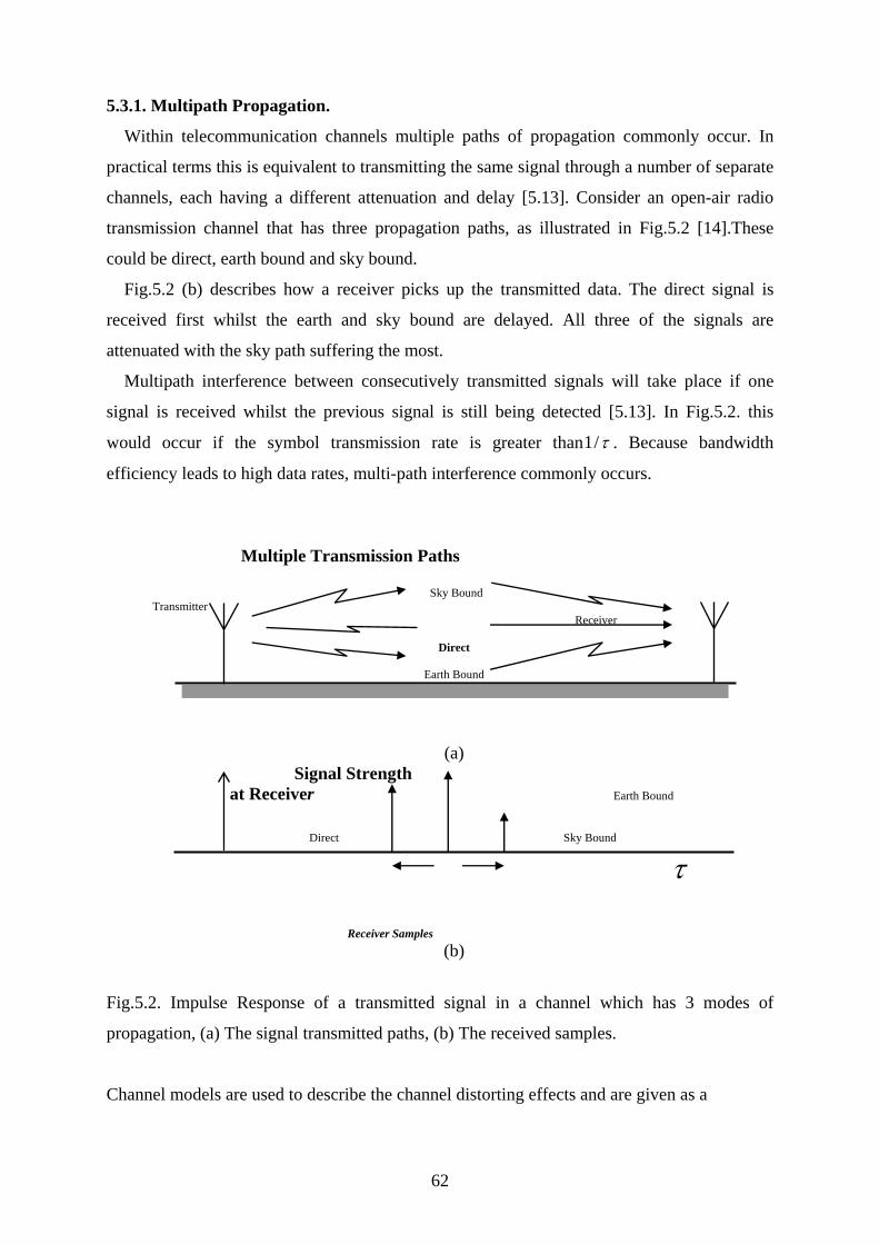
5.3.1. Multipath Propagation.
Within telecommunication channels multiple paths of propagation commonly occur. In
practical terms this is equivalent to transmitting the same signal through a number of separate
channels, each having a different attenuation and delay [5.13]. Consider an open-air radio
transmission channel that has three propagation paths, as illustrated in Fig.5.2 [14].These
could be direct, earth bound and sky bound.
Fig.5.2 (b) describes how a receiver picks up the transmitted data. The direct signal is
received first whilst the earth and sky bound are delayed. All three of the signals are
attenuated with the sky path suffering the most.
Multipath interference between consecutively transmitted signals will take place if one
signal is received whilst the previous signal is still being detected [5.13]. In Fig.5.2. this
would occur if the symbol transmission rate is greater than1/τ . Because bandwidth
efficiency leads to high data rates, multi-path interference commonly occurs.
Multiple Transmission Paths
Sky Bound Transmitter
Receiver
Direct
Earth Bound
(a) Signal Strength
at Receiver Earth Bound
Direct Sky Bound
τ
Receiver Samples
(b)
Fig.5.2. Impulse Response of a transmitted signal in a channel which has 3 modes of
propagation, (a) The signal transmitted paths, (b) The received samples.
Channel models are used to describe the channel distorting effects and are given as a
62

summation of weighted time delayed channel inputs ( )d n i− .
phase channel is convergent, illustrated by
1 2
0( ) ( ) ( ) ( 1) ( 2) ......
mi
i
H z d n i z d n d n z d n z− − −
=
= − = + − + − +∑ (5.1)
The transfer function of a multi-path channel is given in Equation 5.1. The model coefficients
( )d n i− describe the strength of each multipath signal.
5.4. MINIMUM AND NONMINIMUM PHASE CHANNELS
When all the roots of the model z-transform lie within the unit circle, the channel is termed
minimum phase [5.15] The inverse of a minimum
Equation(5.2): 1
1
( ) 1.0 0.51 1( ) 1.0 0.5
H z z
H z z
−
−
= +
=+
0
12
ii
iz
∞−
=
⎛ ⎞= −⎜ ⎟⎝ ⎠
∑(5.2)
nels are not convergent, as shown in
Equation (5.3)
1 2 31 0.5 0.25 0.125z z z− − −= − + − +
ase chanwhere as the inverse of non-minimum ph
1
0 2i=
2 3.5 0.25 0 5z z z ⎤+ −
( ) 0.5 1.01( ) 1.0 0.5
1.
. 1 0 .12
ii
H z zz
H z z
z z
z
−
∞−
= +
=+
⎡ ⎤⎛ ⎞= −⎢ ⎥⎜ ⎟⎝ ⎠
⎡= −⎣ ⎦
∑ (5.3)
Since equalizers are de inve e c annel istortio
model the channel inverse. The minimum phase hannel has a linear inverse model therefore
a linear equalization solution exists. However, limiting the inverse model to m-dimensions
will that non-linear solutions can provide a
perior inverse model in the same dimension.
phase model, where
nger delays are necessary to provide a reasonable equalizer. Equation (5.4) describes a non-
e. The
latter of these is the more suitable form for a linear filter.
⎢ ⎥⎣ ⎦
signed to rt th h d n process they will in effect
c
approximate the solution and it has been shown
su
A linear inverse of a non-minimum phase channel does not exist without incorporating
time delays. A time delay creates a convergent series for a non-minimum
lo
minimum phase channel with a single delay inverse and a four sample delay invers
63

1( ) 0.5 1.0H z z−= +
1 2 31 1 1 0.5 0.25 0.125 (( ) 1 0.5
z z z z non caH z z
− = = − + − ++
.5. INTERSYMBOL INTERFERENCE
overlapping of the
imensionality of the channel output vector helps characterize the multipath
propagation. This has the effect of not only increasing the number of symbols but also
increases the Euclidean distance between the output classes.
When additive Gaussian noise
)usal 5.4)
4 3 2 11 0.5 0.25 0.125 ( )( )
z z z z z truncated and causalH z
− − − −= − + − +
5
Inter-symbol interference (ISI) has already been described as the
transmitted data. It is difficult to recover the original data from one channel sample
dimension because there is no statistical information about the multipath propagation.
Increasing the d
, η , is pre
Gaussian clusters around the symbol centers. These symbol clusters can be characterized by a
probability density function (pdf) with a noise variance
sent within the channel, the input sample will form
2ησ , where the noise can cause the
f the input samples. Error control coding schemes can be employed in such
cases but these often require extra bandwidth.
5.5.1. Symbol Overlap.
The expected number of errors can be calculated by considering the amount of symbol
interaction, assuming Gaussian noise. Taking any two neighboring symbols, the cumulative
distribution function (CDF) can be used to describe the overlap between the two noise
symbol clusters to interfere. Once this occurs, equalization filtering will become inadequate
to classify all o
characteristics. The overlap is directly related to the probability of error between the two
symbols and if these two symbols belong to opposing classes, a class error will occur.
Figure 2.3 shows two Gaussian functions that could represent two symbol noise
distributions. The Euclidean distance, L, between symbol canters and the noise variance, 2σ ,
can be used in the cumulative distribution function of Equation (5.5) to calculate the area of
overlap between the two symbol noise distributions and therefore the probability of error, as
in Equation (5.6) 2
2
1( ) exp22
x xCDF x dxσπσ−∞
⎡ ⎤= −⎢ ⎥
⎣ ⎦ ∫ (5.5)
64

Area of overlap = Probability of error
Fig.5.3. Interaction between two neighboring symbols.
( ) 22LP e CDF ⎛ ⎞= ⎜ ⎟
⎝ ⎠ (5.6)
Since each channel symbol is equally likely to occur, the probability of unrecoverable errors
occurring in the equalization space can be calculated using the sum of all the CDF overlap
between each opposing class symbol. The probability of error is more commonly described
as the BER. Equation(5.7)describes the BER based upon the Gaussian noise overlap, where
spN is the number of symbols in the positive class, mN is the number of number of symbols
in the negative class and iΔ , is the distance between the thi positive symbol and its closest
neighboring symbol in the negative class.
1
2( ) log2
in
isp m n
BER CDFN N
σσ=
= ⎢ ⎥spN ⎤⎛ ⎞Δ⎡
⎜ ⎟+⎢ ⎥⎝ ⎠
ymbol
ai
eeps the research going on to introduce new algorithms to train
the equalizer. The optimal BER equalization
sequence estimator (MLSE) on the entire transmitted data sequence [5.18].A more practical
⎣ ⎦∑ (5.7)
5.6. CHANNEL EQUALIZATION
High speed communications channels are often impaired by channel inter s
interference (ISI) and additive noise. Adaptive equalizers are required in these
communication systems to obtain reliable data transmission. In adaptive equalizers the m n
constraint is training the equalizer. Many algorithms have been applied to train the equalizer,
each having their own advantages and disadvantages. More over the importance of the
channel equalization always k
performance is obtained using a maximum likelihood
65

MLSE would operate on smaller data sequences but these can still be computationally
xpensive, they also have problems tracking time-varying channels and can only produce
quences of outputs with a significant time delay. Another equalization approach
plements a symbol-by-symbol detection procedure and is based upon adaptive filters. The
mbol-by-symbol approach to equalization applies the channel decision
lassifier that separates the symbol into their respective classes. Two types of symbol-by-
mbol equalizers are examined in this thesis, the transvers decision feedback
q linear filters, LTE
nd LDFE, with a simple FIR structure. The ideal equalizer will model the inverse of the
hannel model but this does not take into account the effect of noise within the channel.
e
se
im
sy output samples to a
c
sy al (TE) and
e ualizer (DFE). Traditionally these equalizers have been designed using
a
c
Noise
A basic block diagram of channel equalization is shown in Fig. 5.4.The transmitted signal
X(n) pass through the channel .The block N.L accounts for the nonlinearity associated with
the channel. q(n) is the Gaussian noise added through the channel. The equalizer is placed at
the receiver end. The output of the equalizer is compared with the delayed version of the
transmitted signal to calculate the error signal e(n),which is used by the update algorithm to
update the equalization coefficient such that the error becomes minimum.
∑
Channel
Update Algorithm
+ N.L.
+
y (n)
d(n)
_
X(n)
e(n)
Equalizer
a(n) b(n)
r(n)
q(n)
Delay
N.L. =Nonlinearity
Fig.5.4. Block diagram of Channel Equalization
66

5.6.1. Transversal Filter
The transversal equalizer uses a time-delay vector, ( )Y n (Equation (5.8)), of channel
output samples to determine the symbol class. The {m} TE notation used to represent the
transversal equalizer specifies m inputs.
( ) [ ( ), ( 1), .... , ( ( 1))]Y n y n y n y n m= − − − (5.8)
The equalizer filter output will be classified through a threshold activation device (Fig. 5.5)
so that the equalizer decision will belong to one of the BPSK states i.e. 1 or -1.
z-1 z-1 z-1 z-1y(n) y(n-2) y(n-3) y(n-1) y(n-4) w2(n) w3(n) w4(n) w1(n) w5(n) Adder
d(n)
Fig.5.5. Linear Transversal Filter
y(n)= Received samples
d(n)=Equalized output
1( ) 1.0 0.5H z z−= +Considering the inverse of the channel that was given in Equation (5.3),
is is an infinitely long convergent linear series: 0
1 1( ) 2
ii
i
zH z
∞−
=
⎛ ⎞= −⎜ ⎟⎝ ⎠
∑th . Each coefficient of
this inverse model can be used in a linear equalizer as a FIR tap-weight. Each tap-dimension
will improve the accuracy; however, high input dimensions leave the equalizer susceptible to
noisy samples. If a noisy sample is received, this will remain within the filter affecting the
output from each equalizer tap. Rather than designing a linear equalizer, a non-linear filter
can be used to provide the desired performance that has a shorter input dimension; this will
reduce the sensitivity to noise.
67

5.7. SIMULATION RESULTS
BP algorithm and a linear FIR equalizer with LMS
algorithm as discussed in section 2.6.. Th
e simulations
e assign the same input signals to the two neural-network based equalizer structures
onsidered. To the channel output a zero mean white Gaussian noise of SNR 30dB was
dded. Th ei s is to s the SNR equal to the
c ocal of noise varian t of the equ
Fo NN th zer h branch each s expanded to five branches
sing trigonometric functions. The output of the FLANN contains a tanh(.) function. Total
umber of weights used for FLANN is 31 (including one bias term).In case of CFLANN in
e first stage each branch is expanded into five branches. The output of first s gain
xpanded into three terms. The number of weights used in the first stage is 19 (including one
ias term). The number of weights used in the second stage is 4 (including one bias term).
otal number of weights used for FLANN is 23. At each stage CFLANN contains tanh(.)
nction. The l as 0.03 for both the structure. To study the BER
erformance, each of the equalizer structures was trained with 5000 iterations for optimal
eight solution. After comple qualizer was carried out. The
ER was calculated 105 data samples.
The channel considered here has the normalized transfer function given in z-transform
the nonlinearity is plotted in Fig.5.6.From the BER plot it is
bserved that the performance of CFLANN equalizer is better than those of FLANN and
MS based equalizers.
Extensive simulation studies have been carried out for channel equalization problem as
described in Fig 5.4. using the two discussed ANN structures (FLANN and CFLANN), as
discussed in section 3.4. and 3.5., with
e digital message was with binary phase shift
keying (BPSK) signal constellation and in the form [-1 1] in which each symbol was
obtained from a random distribution. To obtain meaningful comparisons from th
w
c
a e rec ved ignal power normalized unity so a to make
re ipr ce at the inpu alizer.
r FLA e equali ave six es and branch i
u
n
th tage is a
e
b
T
fu earning rate is chosen
p
w tion of the training, testing of the e
B
form: 1 2( ) 0.26 0.93 0.26H z z z− −= + + (5.9)
The following types of nonlinearity were introduced in the channel.
(1) 2 3( ) ( ) 0.2 ( ) 0.1 ( )b n a n a n a n= + − (5.10)
(2) 2 3( ) ( ) 0.2 ( ) 0.1 ( ) 0.5cos( ( ))b n a n a n a n a nπ= + − + (5.11)
The BER performance for both
o
L
68

10 12 14 16 18 20 2210-5
10-4
10-3
10-2
10-1BER plot
lmsflanncflann
BE
R---
--->
SNR in dB----->
(a)
10 11 12 13 14 15 16 17 18 19 2010-5
10-4
10-3
10-2
10-1BER plot
lmsflanncflann
BE
R---
-->
SNR in dB----->
plot (a) For nonlinearity(5.10) (b) For nonlinearity(5.11)
(b)
Fig.5.6. BER
69

5.8. SUMMARY
To compensate the effect of ISI and other type noises on the bits, when transmitted through
the channel, an equalizer is placed at the receiver end. For the equalization of highly
nonlinear systems the number of branches in the FLANN increases. Even some cases give
poor performance. To decrease the number of branches and increase the performance a two-
stage FLANN is described in this chapter. Here the output of the first stage again undergoes
functional expansion. From the BER plots it can be observed that for nonlinear channels the
performance of CFLANN equalizer is considerably better than those of FLANN and LMS
based equalizers.
70

Chapter 6
CONCLUSIONS

6. CONCLUSIONS
ctures, MLP, FLANN and CFLANN, are discussed. Due to multilayer
ructure of the MLP, its convergence is slow. On the otherhand FLANN is a single layer
ructure with functionally mapped inputs. Here, the initial representation of a pattern is
nhanced by using nonlinear function and thus the pattern dimension space is increased. The
nctional link acts on an element of a pattern or entire pattern itself by generating a set of
nearly independent function and then evaluates these functions with the pattern as the
rgument. Hence separation of the patterns becomes possible in the enhanced space. While
onstructing an artificial neural network the designer is often faced with the problem of
hoosing a network of the right size for the task to be carried out. To overcome this problem
GA based pruning strategy and weight updation algorithm is used.
Transmission bandwidth is one of the precious resources in digital communication
stems. To achieve better use of this resource, signals are commonly transmitted through
and-limited channels. So the received signals inevitably affected by inter symbol
terference(ISI). A channel equalizer is used to recover the transmitted data from the
ceived signals. If the nonlinearity associated with the system or channel is high the number
f branches in the FLANN increases. Even some cases give poor performance. To decrease
e number of branches and increase the performance CFLANN is used.
.2. SCOPE FOR FUTURE WORK
In this thesis CFLANN is used for only FIR system and channels. This can be extended to
finite impulse response (IIR) systems and channels.
In pruning technique GA is used which is a very slow process and has a very high
omputational complexity. Hence research can be done to find out a faster method for
runing.
6.1. CONCLUSIONS
The aim of this thesis is to find a proper artificial neural network (ANN) model for adaptive
nonlinear system identification and channel equalization. The prime advantages of using
ANN models are their ability to learn based on optimization of an appropriate error function
and their excellent performance for approximation of nonlinear functions. .
Three ANN stru
st
st
e
fu
li
a
c
c
a
sy
b
in
re
o
th
6
in
c
p
71

REFERENCES
Chapter. 1 [1.1] Narendra K.S. and Annaswamy A.M., Stable Adaptive Systems. Englewood Cliffs,
NJ: Prentice - Hall, 1989.
[1.2] Proakis J. G.,
Digital Communications, third edition, McGraw Hill, 1995.
[1.3] Chen S.,Billings, S. A. and Grant, P. M.,“Nonlinear system identification using
neural networks”, Int. J. Contr., vol. 51, no. 6, June 1990, pp. 1191-1214.
[1.4] Narendra K. S. and Parthasarathy K., “Identification and control of dynamic systems
using neural networks”,
IEEE Trans. on Neural Networks, vol. 1, Mar, 1990, pp. 4-27.
[1.5] Widrow B. and. Stearns S. D., Adaptive Signal Processing, Second Edition, Pearson
Education, 2002.
[1.6] Qureshi S., “Adaptive equalization”, IEEE Communications Magazine, Mar 1982, pp
9-16.
[1.7] Siller C., “Multipath propagation”, IEEE communications magazine, vol.22, no.2,
Feb.1984, pp.6-15.
[1.8] Chen S., Mulgrew B. and McLaughlin S., “Adaptive Bayesian Equalizer with
Decision Feedback”, IEEE Trans. on Signal Processing, vol.41, no.9, Sept. 1993,
pp.2918-2927.
[1.9] Patra J. C., Pal R. N., Chatterji B. N. and Panda G., “Identification of nonlinear
dynamic systems using functional link artificial neural networks”, IEEE Trans. On
Systems, Man and Cybernetics-part B: Cybernetics, vol. 29, no. 2, April 1999, pp.
254-262.
Chapter. 2 [2.1] Ljung L., System Identification. Englewood Cliffs, NJ: Prentice-Hall, 1987.
[2.2] Akaike H.,“A new look at the statistical model identification”. IEEE Trans. on
Automatic Control, AC-19:716-723, 1974.
[2.3] Widrow Bernard & D.Streans Samuel, Adaptive Signal Processing, Second Edition,
Pearson Education, 2002.
72
[2.4] Haykin Simon, Adaptive Filter Theory, Pearson Education Publisher, 2003.
[2.5] Wiener N., “Extrapolation, Interpolation, and Smoothing of Stationary Time Series
with Engineering Applications”, MIT Press, vol.15.pp.18-25, Cambridge, MA, 1949.
n N., “The Wiener RMS (root-mean-square) error criterion in filter design and [2.6] Levinso
prediction”, Math Phys., pp. 261-278, Vol.25, 1947.
Fan H. and Jenkins, W.K. "A[2.7] New Adaptive IIR Filter", IEEE Trans. on Circuits and
Systems, vol. CAS-33, no. 10, Oct. 1986 , pp. 939-947.
[2.8] Ho K.C. and Chan Y.T., "Bias Removal in Equation-Error Adaptive IIR Filters", IEEE
Trans. on Signal Processing, vol. 43, no. 1, Jan. 1995.
[2.9] Cousseau J.E. and Diniz P.S.R., "New Adaptive IIR Filtering Algorithms Based on the
Steiglitz-McBride Method", IEEE Trans Signal Processing, vol. 45, no. 5, May 1997.
[
regational Gradient Descent", Mathematics of Control, Signals, and
2.10] Blackmore K.L., Williamson R.C., Mareels I.M.Y and Sethares, W.A., "Online
Learning via Cong
Systems vol.10, pp. 331-363,1997.
Haykin[2.11] Simon, “Adaptive Filter Theory”, Third Edition, Prentice-Hall Inc., Upper
[2.12] Nambiar, R., “Learning Algorithms: Theory and Applications
in Signal Processing, Control, and Communications”, CRC Press
Saddle River, NJ, 1996.
Mars P., Chen J.R. and
, vol.10,pp.18-25Inc.,
Chapter. 3 [3.1] Haykin S.,“
1996.
NeuralNetworks: A ComprehensiveFoundation”, Pearson Education Asia,
S., Lewis F.L.,“Identification of a class of nonlinear dynamical systems
ultilayered neu
2002.
[3.2] Jagannathan
using m ral networks”, IEEE International Symposium on Intelligent
Control, Columbus, Ohio, USA, 1994), pp. 345–351.
a K. S., and Parthasarathy K., “Identification and control of dynamical system [3.3] Narendr
using neural networks,” IEEE Trans. on Neural Networks, vol. 1, no.1, Mar. 1990,
[3.4] P Neural Network
pp. 4-26.
ao Y. H., Adaptive Pattern Recognition and , Reading, MA, Addison
Wesley, 1989, Chapter 8, pp.197-222.
73

[3.5] Patra J.C., Pal R.N., Chatterji B.N., and Panda G., “Identification of Nonlinear
Dynamic Systems Using Functional Link Artificial Neural Networks”, IEEE Trans.
on Systems, Man and Cybernetics-Part B : Cybernetics Vol. 29, No.2, Apr.
[3.6] P Identification Using Chebyshev
1999,pp.254-262.
atra J.C., Kot A.C.,“Nonlinear Dynamic System
Functional Link Artificial Neural Networks”, IEEE Trans. on Systems Man and
Cybernetics-Part B. Cybernetics.Vol.32,No.4,Aug. 2002,pp.505-510.
D ans. on circuits and systems-I:
[3.7] Wang J.and Chen Y., “A Fully Automated Recurrent Neural Network for Unknown
ynamic System Identification and Control”, IEEE Tr
Regular papers, Vol.53, No.6, June 2006 pp.1363-1372..
artin T. Hagan, Howard B. Demuth., [3.8] M Neural Network Design, Thomson Learning
[3.9] D
2003.
ayhoff E.J.,“Neural Network Architecture – An Introduction” Van Norstand Reilold,
ew York, 1990. N
[3.10] Bose N.K., and Liang P., “Neural Network Fundamentals with Graphs, Algorithms,
Applications”, TMH Publishing Company Ltd, 1998.
idrow Bernard and D.Streans Samuel. [3.11] W Adaptive Signal Processing, Pearson
Education Publisher.
[3.12] Park G.H. and Sobjic D.J., “Learning and Generalization Characteristics of
dom Vector Function”, Neuro Computation
Pao Y.H.,
the Ran , vol.6, pp.163-180, 1994.
l Equalization”, Signal Processing 43(1995)
[3.13] Patra J.C., and Pal R.N., “A Functional Link Artificial Neural Network for Adaptive
Channe , vol.43, no.2, pp.181-195May
[3.14] VDT and Its
1995.
Mishra S. K. and Panda G., “A Novel Method for Designing L
Comparison with Conventional Design”, SAS 2006-IEEE Senosrs Applications
Symposium,pp.129-134, Houstan, Texas, USA, 7-9 Feb.2006
[4.1] nd Artificial Systems
Chapter. 4 Holland J.H., Adaptation in Natural a . University of Michigan
Press, Ann Arbor, 1975.
74

[4.2] Holland J. H., “Outline for a logical theory of adaptive systems,” J. ACM, vol. 3, pp.
297 - 314, July 1962; also in A. W. Burks, Ed., Essays on Cellular Automata, Univ.
Illinois Press, 1970, pp. 297-319.
DeJong K. A., “A[4.3] n analysis of the behavior of a class of genetic adaptive systems,”
Ph.D. dissertation (CCS), Univ. Mich., Ann Arbor, MI, 1975.
Fitzpatrick J. M., Grefenstette J. J., and Gucht D. Van, “Image registration by genetic
search,”
[4.4]
in Proc. IEEE Southeastcon ’84, 1984, pp.460-464.
[4.5] Goldherg D. E. and Lingle R., ‘‘Alleles, loci and the traveling salesman problem,” in
Proc. Int. Conf. Genetic Algorithms and Their Appl., pp. 154-159. 1985
Grefenstette J. J., Gopal R., Rosmaita B. and VanGucht[4.6] D., “Genetic algorithms for
the traveling salesman problem,” in Proc. Int. Conf Genetic Algorithms and Their
Applications, pp. 160-165, 1985.
rints from the Proc. 19th annual Pittsburgh Conf Modeling and
[4.7] Das R. and Goldberg D.E., “Discrete-time parameter estimation with genetic
algorithms,” prep
Simulation, 1988.
nf Acoustics, Speech, Signal
[4.8] Etter D. M., Hicks M. J. and. Cho K. H, “Recursive adaptive filter design using an
adaptive genetic algorithm,” Proc. IEEE Int. Co
Processing, vol. 2, pp. 635-638, 1982.
Goldberg D. E. System[4.9] identification via genetic algorithm, unpublished manuscript,
Univ. Mich., Ann Arbor, MI, 1981.
Kristinsson K. and Dumont G. A.,” Genetic algorithms in system identif[4.10] ication,”
Third IEEE Int. Symp. Intelligent Contr., Arlington, VA, pp. 597-602, 1988.
Smith T. and DeJong K.A., “Genetic Algorithms applied to the calibration of
inform
[4.11]
ation driven models of US migration patterns,” in Proc. 12th Annu. Pittsburgh
Conf Modeling and Simulation, 1981, pp. 955-959, 1981.
[4.12] Giles C. Lee and Christian W. Omlin, “Pruning Recurrent Neural Networks for
Improved Generalization Performance”, IEEE Trans. on Neural Networks Vol.5,
No.5, Sept.1994,pp.848-851.
[4.13] Markel J.D., “FFT pruning”, IEEE Trans. on Audio and Electro Acoustics, Vol.AU-
4, Dec.1971,pp.305-311.
[
l Letter Reduction”, IEEE conference
19, No.
4.14] Jearanaitanakij K.and Pinngern O., “Hidden Unit Reduction of Artificial Neural
Network on English Capita , pp.1-5. June 2006.
75

4.15] Chung T., Leung H., “A genetic algorithm approach in optimal capacitor selection with
harmonic distortion considerations”, International Journal of Electrical Power & Energy
Systems, vol.21, no.8, Nov. 1999, pp
[
.561-9.
[4.16] Fogel D., “What is evolutionary computing”, IEEE spectrum magazine, Feb. 2000,
pp.26-32.
[4.17] Goldberg D., Genetic algorithms in search optimization , Addison-Wesley, 1989.
C[5.1] transmission
hapter. 5 Arcens S., Sueiro, J. C. and Vidal, A. R. F. "Pao networks for data
equalization," Proc. Int. Jt. Conf. on Neural Networks, Baltimore, Maryland, pp.
11.963-11.968, June 1992.
Chen S., Gibson G.J., Cowan, C
[5.2] .F.N. and Grant P. M., “Adaptive equalization of
finite nonlinear channels using multilayer perceptrons,” EURASIP Signal Processing
Jnl., V01.20, 1990, pp.107-119.
Chen S., Gibson G[5.3] .J. and Cowan C.F.N., "Adaptive channel equalization using a
polynomial perceptron structure," Proc.IEE, Pt.I, Vo1.137, pp.257-264. October 1990.
Gan W. S., Saraghan J. J., and Durrani T. S., "New functional-link based equalizer", [5.4]
Electronics Letters, Vol.28, No. 17, 13 Aug. 1992, pp. 1643-1645.
[5.5] Haykin S., Adaptive Filter Theory, Prectice Hall, Englewood Cliffs, NJ. 1986,
Chapter 5, pp.194-268.
[5.6] Hornik K., Stichcombe M. and White H.,"Multilayer feed forward networks are
universal approximators", IEEE Trans. on Neural Networks, Vol. 2, 1989, pp. 359-
[5.7]
366.
Meyer M. and Pfeiffer G.,"Multilayer perceptron based decision feedback equalizers
for channels with intersymbol interference,"Proc. IEE, Pt- I ,Vol 140, No 6, pp 420-
[5.8]
424,June 1992.
Pao Y. H. Adaptive Pattern Recognition and Neural Networks, Reading, MA,
Addison Wesley, 1989, Chapter 8, pp. 197-222, Dec 1993.
P Signal Processing Jnl
[5.9] Patra J. C. and Pal R. N.,"A functional link artificial neural network for adaptive
channel equalization", EURASI ., Vol. 43, No. 2, 1995
[5.10] ,
madaline and back propagation," Proc. IEEE
.pp.662-670.
Widrow B. and Lehr, M. A.,"30 years of adaptive neural networks: perceptron
, vo1.78, No.9, September 1990,
pp.1415-1442.
76

[5.11] Lucky R. W., "Automatic equalization for digital communications", Bell Syst. Tech.
Journal, vol. no. 44, April 1965, pp. 547-588.
Proakis J. G., [5.12] Digital Communications, third edition, McGraw Hill, 1995.
[5.13] Qureshi S., “Adaptive equalization”, Proceedings of the IEEE, vol.73, no.9, pp.1349-
1387, Sept. 1985.
[5.14] Widrow B., Stearns S., Adaptive signal processing, Chap.9, Prentice-Hall Signal
processing series, New Jersey 1985.
i O., “Adaptive processing, the least mean squares approach with [5.15] Macch
applications in transmission”, John Wiley and Sons, West Sussex. England, 1995.
Siu S., “Non-linear Adaptive Equalization based on multi-layer perceptron
Architecture”,
[5.16]
Faculty of Science, University of EdinburghPh.D. Thesis, , 1990.
77