אוניברסיטת בן-גוריון

Ram Brustein

Introduction: The case for

closed string moduli as inflatons Cosmological stabilization of moduli

Designing inflationary potentials (SUGRA, moduli)

The CMB as a probe of model parameters

with I. Ben-Dayan, S. de AlwisTo appear

============Based on:

hep-th/0408160with S. de Alwis, P. Martens

hep-th/0205042 with S. de Alwis, E. Novak

Models of Modular Inflation

Stabilizing closed string moduli• Any attempt to create a deSitter like phase will induce a

potential for moduli

• A competition on converting potential energy to kinetic energy, moduli win, and block any form of inflation

241

2/14)4( ))(( AFRgxdS

3214)4(

eRgxdS

Inflation is only ~ 1/100 worth of tuning away!(but … see later)

Generic properties of moduli potentials:

• The landscape allows fine tuning• Outer region stabilization possible• Small +ve or vanishing CC possible • Steep potentials• Runaway potentials towards

decompactification/weak coupling• A “mini landscape” near every stable mininum +

additional spurious minima and saddles

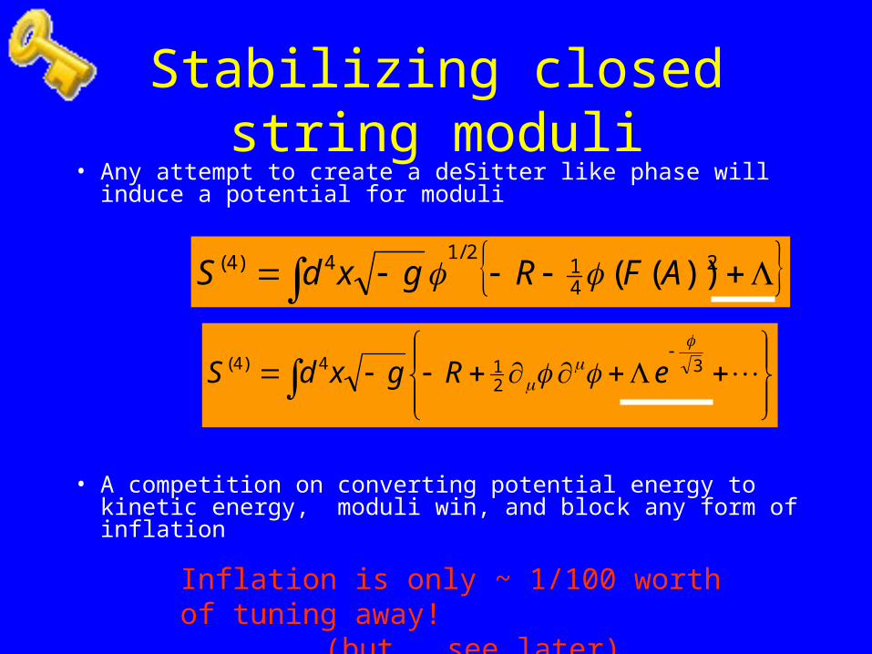
Cosmological stability

• The overshoot problem hep-th/0408160

Proposed resolution:role of other sources

• The 3 phases of evolution

– Potential push: jump

– Kinetic : glide

– Radiation/other sources : parachute opens

Previously:Barreiro et al: tracking

Huey et al, specific temp. couplings Inflation is only ~ 1/100 worth of tuning away!

Example: different phases

== potential

== kinetic

== radiation

Example: trapped field

== potential

== kinetic

== radiation

Using cosmological stabilization for designing models of inflation:

• Allows Inflation far from final resting place

• Allows outer region stabilization

• Helps inflation from features near

the final resting place

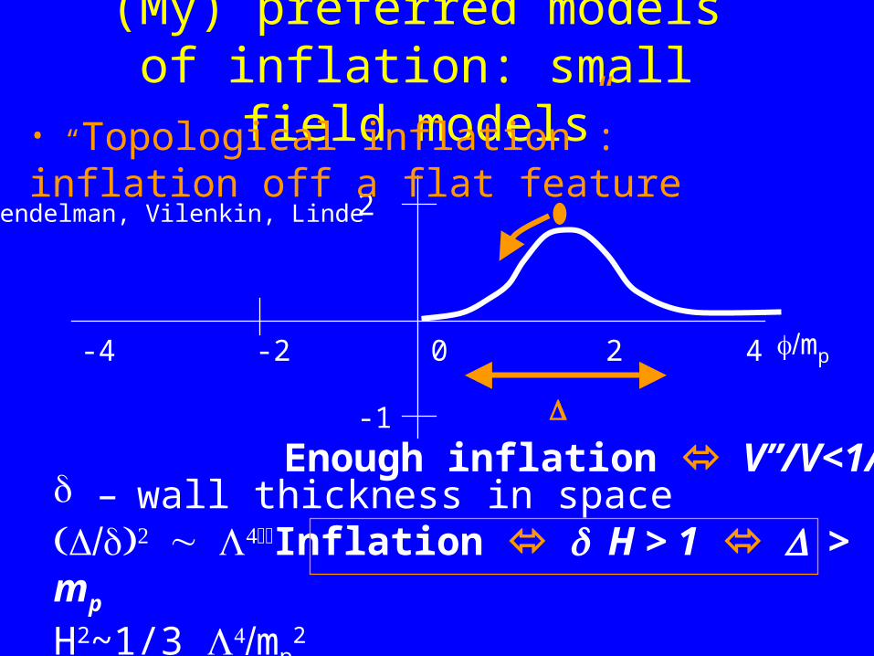
(My) preferred models of inflation: small field models

– wall thickness in spaceInflation H > 1 > mp H2~1/3 mp

2

2

-1

mp-4 -2 0 2 4

• “Topological inflation”: inflation off a flat featureGuendelman, Vilenkin, Linde

Enough inflation V’’/V<1/50

Results and Conclusions: preview

• Possible to design fine-tuned models in SUGRA and for string moduli

• Small field models strongly favored• Outer region models strongly disfavored

• Specific small field models

– Minimal number of e-folds– Negligible amount of gravity waves: all models

ruled out if any detected in the foreseeable future

Predictions for future CMB experiments

Designing flat features for inflation

• Can be done in SUGRA• “Can” be done with steep exponentials alone• Can (??) be done with additional (???) ingredients

(adding Dbar, const. to potential see however ….. ) • Lots of fine tuning, not very satisfactory• Amount of tuning reduces significantly towards

the central region

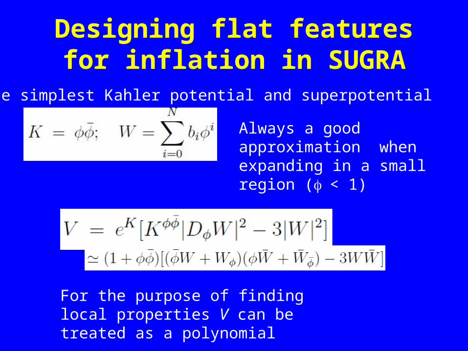
Designing flat features for inflation in SUGRA

Take the simplest Kahler potential and superpotential

Always a good approximation when expanding in a small region (< 1)

For the purpose of finding local properties V can be treated as a polynomial

Design a maximum with small curvature with polynomial eqs.

Needs to be tuned for inflation

Design a wide (symmetric) plateau with polynomial eqs.

A simple solution: b2=0, b4=0, b1=1,b3=/6,

b5 determined approximately by (*)

(*)

In practice creates two minima @ +y,-y

Designing flat features for inflation in SUGRA

The potential is not sensitive to small changes in coefficientsIncluding adding small higher order terms, inflation is indeed 1/100 of tuning away

-0.6 -0.4 -0.2 0.2 0.4 0.6

-0.5

0.5

1

1.5A numerical example:

b2=0, b4=0, b1=1,b3=/6,

b5 y4(y2+5) + y2+1=0

b1 b3 – 2(b0)2

Need 5 parameters:V’(0)=0,V(0)=1,V’’/V=DTW(-y), DTW(+y) = 0

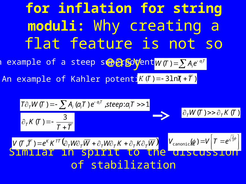
• An example of a steep superpotential Tai

ieATW )(

1:,)()( TasteepeTaATWT iTa

iiTi

)ln(3)( TTTK

TTTKT

3

)()()( TKTW TT

• An example of Kahler potential

Similar in spirit to the discussion of stabilization

WKKWWWKeTTV TTTTTTTTK ),(

3

2

)(canonical eTVV

Designing flat features for inflation for string moduli: Why creating a

flat feature is not so easy

• extrema• min: WT = 0• max: WTT = 0• distance T

Why creating a flat feature is not so easy (cont.)

WKKWWWKeTTV TTTTTTTTK ),(

Example: 2 exponentials

WT = 0

WTT = 0

0212211 TaTa eaAeaA

021 222

211 TaTa eaAeaA

211

222

12max ln

1

aA

aA

aaT

11

22

12min ln

1

aA

aA

aaT

1

2

12minmax ln

1

a

a

aaTTT

21

11

aaT For (a2-a1)<<a1,a2

21max

aaV

V

T

TT

1))(( max2max1can

''can

max

TaTaV

V

11

max1max

TaT

T

For (a2-a1)<<a1,a2

1))(( max2max1can

''can

max

TaTaV

V

11

max1max

TaT

T

Amount of tuning

To get ~ 1/100 need tuning of coefficients @ 1/100 x 1/(aT)2

The closer the maximum is to the central area the less tuning.Recall: we need to tune at least 5 parameters

Designing flat features with exponential superpotentials

Need N > K+1 (K=5N=7!) unless linearly dependent

Trick: compare exponentials to polynomials by expanding about T = T2

Linear equations for the coefficients of

Numerical examples

2.5 2.75 3.25 3.5 3.75

2

4

6

8

10

2 4 6 8 10 12 14

10

20

30

40 7 (!) exponentials + tuning ~ (aT)2 = UGLY

Lessons for models of inflation

• Push inflationary region towards the central region

• Consequences:– High scale for inflation– Higher order terms are important, not

simply quadratic maximum 2.4 2.6 2.8 3.2 3.4 3.6

0.94

0.95

0.96

0.97

0.98

0.99

2.5 2.75 3.25 3.5 3.75

2

4

6

8

10

Phenomenological consequences

• Push inflationary region towards the central region

• Consequences:– High scale for inflation– Higher order terms are important, not

simply quadratic maximum

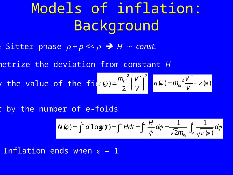
Models of inflation: Background

de Sitter phase + p << const.

Parametrize the deviation from constant H22

2)(

V

Vmpl )()( 2

V

Vmpl

Or by the number of e-folds

ei

eieiei

dm

dH

HdttadNpl

t

t

t

t )(

1

2

1)(log)(

by the value of the field

Inflation ends when = 1

Models of inflation:Perturbations• Spectrum of scalar perturbations

• Spectrum of tensor perturbations

aHkm

HkP

pl

12)(

2

aHkm

HkP

plT

2

2)(

Tensor to scalar ratio (many definitions)r is determined by PT/PR , background cosmology, & other effectsr ~ 10 (“current canonical” r =16 )

Spectral indices

r = C2Tensor/ C2

Scalar (quadropole !?)

CMB observables determined by quantities ~ 50 efolds before the end of inflation

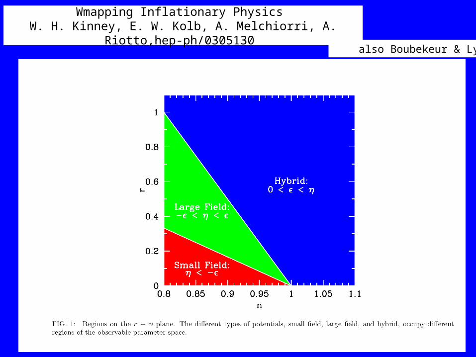
Wmapping Inflationary Physics W. H. Kinney, E. W. Kolb, A. Melchiorri, A. Riotto,hep-ph/0305130

See also Boubekeur & Lyth

Simple example:

The “minimal” model: – Quadratic maximum

– End of inflation determined by higher order terms

2max3

2max2

4 1~)( aaV

Minimal tuning minimal inflation, N-efolds ~ 60 “largish scale of inflation” H/mp~1/100

Sufficient inflation enoughsmallmax init

6/1)('' max2max VHinit Qu. fluct. not too large

For example:

The “minimal” model: – Quadratic maximum

– End of inflation determined by higher order terms

2.4 2.6 2.8 3.2 3.4 3.6

0.94

0.95

0.96

0.97

0.98

0.99

2max3

2max2

4 1~)( aaV

Unobservable!

'' ( ).92 .08(25 | | 1)

( )

0.01

CMBS

CMB

Vn

V

r

CMB

CMBCMBS

r

n

16

241

2 4( '/ ) ~ 0.01

~ 1/ 25 0CMB

CMB

V V

Expect for the whole class of models

1/2 < 25|V’’/V| < 1 .92 .96

0.01Sn

r

WMAP

Detecting any component of GW in the foreseeable future will rule out this whole class of models !

Summary and Conclusions

• Stabilization of closed string moduli is key

• Inflation likely to occur near the central region

• Will be hard to find a specific string realization

• Specific class of small field models – Specific predictions for future CMB experiments