Embed Size (px)
Citation preview
:_NASA-_T_nical
-1996
-_-March 1982
" - r ,
. ,,-, _ .
=
_r " . " .
. " '.
-\
Self-Tuning Regulatorsfor Multicyclic Controlof Helicopter Vibration
Wayne Johnson
https://ntrs.nasa.gov/search.jsp?R=19820012314 2020-04-12T18:05:49+00:00Z


NASATechnicalPaper1996
1982
RI/ ANahonal Aeronauhcsand Space Administration
Scientific and TechnicalInformation Branch
Self-Tuning Regulatorsfor Multicyclic Controlof Helicopter Vibration
Wayne Johnsond rues Research Center
MoIfett Field, Ca li[ornia


TABLE OF CONTENTS
INTRODUCTION .................................
Previous Work .............................
Scope of Present Investigation ......................
HELICOPTER MODEL .............................
IDENTIFICATION ................................
Least-Squares Method ...........................
Generalized Least-Squares Method .....................
Recursive Parameter Identification ....................
Recursive Generalized Least Squares ...................
Exponential Window ............................
Kalman-Filter Identification .......................
Identifiability .............................
Starting Recursive Algorithms ......................
Numerical Implementation .........................
CONTROL ....................................
Performance Function ..........................
Deterministic Controller .........................
Controller Dynamics ..........................
Controller Gain Update .........................
Cautious Controller ..........................
Dual Controllers .............................
REGULATORS ..................................
Classification ..............................
Previous Work ..............................
ANALYSIS AND SIMULATION ...........................
Open-Loop Control ............................
Closed-Loop Control ..........................
Caution and Learning ...........................
Adaptive Identification .........................
Identifiability ............................
Adaptive Open-Loop Regulator .......................
CONCLUSIONS ..................................
RECOMMENDATIONS ................................
REFERENCES ..................................
Page
1
i
2
6
8
9
9
i0
ii
ii
13
15
16
16
16
17
18
20
21
23
24
24
26
29
29
30
33
34
37
38
40
41
43
iii


NOMENCLATURE
C controller gain (response feedback)
CAe controller gain, due to control-rate limit
CO controller gain, due to control-magnitude limit
f factor defining functional dependenceof r, P, and Q on
J quadratic performance function
k,k z Kalman-filter or recursive algorithm gain
L
M
m
N
P
P
Q
q
R
r
T
t
U
V
W
Wz
WZXO
Wo
W z
Z
number of parameters identified
a priori error variance matrix
a priori error variance
number of measurements
error variance matrix
error variance
parameter variance matrix
parameter variance
measurement noise variance matrix
measurement noise variance
transfer-function matrix
transpose of row of T matrix; time
random variable describing parameter variation
measurement noise
weighting matrix
weighting matrix in performance function, on response
weighting matrix in performance function, on control rate
weighting matrix in performance function, on control amplitude
weight in performance function
matrix of response-vector measurements
V

z
z 0
At
Az n
AOn
vector of harmonics of response variables
uncontrolled response level
exponential filter parameter
sampling time-step
response increment, zn - Zn_ I
control increment, @n - 8n-I
6nm Kronecker delta function (6 = 1
@
e
00
kc
T
if n = m; zero otherwise)
matrix of control-vector measurements
vector of harmonics of control variables
input 8 required for zero response
eigenvalue
empirical factor in cautious controller
time constant
Subscripts:
j measurement number
n,m time-step
0 initial conditions
Superscript:
T transpose
Special characters:
E( ) expectation
(^) estimate
(-) a priori estimate (before measurement)
vi

SELF-TUNINGREGULATORSFORMULTICYCLICCONTROL
OFHELICOPTERVIBRATION
WayneJohnson
AmesResearch Center
SUMMARY
A class of algorithms for the multicyclic control of helicopter vibration andloads is derived and discussed. This class is characterized by a linear, quasi-static,frequency-domain model of the helicopter response to control; identification of thehelicopter model by least-squared-error or Kalman-filter methods; and a minimumvariance or quadratic performance function controller. Previous research on such con-trollers is reviewed and related to the present work. The derivations and discussionscover the helicopter model; the identification problem, including both off-line andon-llne (recursive) algorithms; the control problem, including both open-loop andclosed-loop feedback; and the various regulator configurations possible within theclass. Conclusions from analysis and numerical simulations of the regulators provideguidance in the design and selection of algorithms for further development, includingwind-tunnel and flight tests.
INTRODUCTION
A class of algorithms for the multicyclic control of helicopter vibration andloads, currently being developed by several investigators, is characterized by (i) alinear, quasi-static, frequency-domain model of the helicopter response to control;(2) identification of the helicopter model by least-squared error or Kalman-filtermethods; and (3) a minimumvariance or quadratic performance function controller.Such a control system combining recursive parameter estimation with linear feedbackis called a self-tuning regulator.
Figure 1 outlines the control task. It is desired to minimize airframe vibra-tion, the loads on the rotating and nonrotating components, and possibly the powerrequirement of the helicopter. The control parameters available are normally thepitch angles of the rotor blades, which are positioned by actuators in the rotatingor nonrotating frame. In steady-state flight, the helicopter vibratory motion isideally periodic, with fundamental frequency _ for componentsin the rotating frameand N_ for componentsin the nonrotating frame (where _ is the rotational speed ofthe rotor, and N is the numberof blades; see Johnson (1980)). Hence the controlrequired to alleviate the vibration and loads will be periodic, and the control systemcan deal with the harmonics of the input and output.
This control is referred to as multicyclic or higher-harmonic control, to dis-tinguish it from the meanand once-per-revolution blade-pitch control (in the rotatingframe) that is required to trim the helicopter. The regulator algorithm consists ofparameter estimation, gain calculation, and the control feedback. Someof these stepsmaybe performed off-line. A digital control system operating on the harmonics of theinput and output is considered here. Hence, the regulator also includes transforma-tions between the time and frequency domains, and between analog and digital

representations of the signals. The present report is concerned with the regulatoralgorithms, so the time-frequency domainand analog-digital transformations are notconsidered further. Moreover, the actuators can be treated by simply including themin the helicopter model. Hencethe simplified system outline in figure 2 is the basisfor the present work. Only self-tuning regulators and related systems are examinedinthis report. Shaw(1980), McCloud (1980a,b), and Johnson (1980) review multicycliccontrol, including other feedback concepts, and discuss helicopter vibration ingeneral.
MULTICYCLIC_
CONTROL
ACTUATORS
(ROTATING OR
NONROTATING
FRAME)
tl
OPERATING
CONDITIONS
HELICOPTER
AIRCRAFT
REGULATOR
I CONSTRUCT
TIME HISTORY,
AND O/A
TIME HISTORY
OF LOADS,
PERFORMANCE.
ANDPOWER
Ir-----
HARMONIC
ANALYSIS,
AND A/D
FEEDBACK _,_CONTROLLER
tGAIN
CALCULATION
t---t k--ESTIMATION
HARMONICSOF
CONTROL
(ROTATING OR
NONROTATING
FRAME)
OPERATING
CONDITIONS
o HEL,COPTER
AIRCRAFT
--_ R_ULATOR-FEEDBACK
CONTROLLER
I GAINCALCULATION
t,.._ PARAMETER F--ESTIMATION
HARMONICS OF
LOADS,
HARMONICS OF
VIBRATION,
POWER
Figure i.- Schematic of helicopter
multicyclic control system.
Figure 2.- Simplified schematic for a
digital frequency-domain control system.
Previous Work
McCloud and Kretz (1974) and Kretz et al. (1973a,b) tested multicyclic control
on a full-scale jet-flap rotor in a wing tunnel. They examined the response of the
blade loads and vibration to control in the rotating frame. They introduced the con-
cept of a linear, quasi-static representation of the rotor response (including the
notation "T" for the transfer function). This transfer function representation was
attributed to J.-N. Aubrun (McCloud and Kretz, 1974). The T-matrix was calculated
from the wind-tunnel data by the least-squares method. Then the open-loop control
required to minimize a quadratic performance function was calculated. McCloud (1975)
applied this method to data obtained by theoretical analysis of a Multicyclic Con-trollable Twist Rotor (MCTR). He considered the reduction of both blade loads and
hub shears, including the influence of the relative weights on the loads and

vibration in the performance function. McCloudand Weisbrich (1978) then applied themethod to data from a wind-tunnel test of a full-scale MCTR. They considered thecontrol required to reduce both blade loads and test module acceleration, includingthe influence of relative weights in the performance index and the sensitivity of thecontrol to the rotor lift. Brown and McCloud (1980) considered reduction of the testmodule vibration, using the data from the MCTRtest again. They examined the influ-ence of the relative weights on the various accelerometers, and the influence ofweights on the control magnitude in the performance function. They examined theinfluence of rotor lift, propulsive force, and speed on the open-loop control.
Sissingh and Donham(1974) tested a model hingeless rotor in a wind tunnel. Theymeasured the vibratory hub momentand vertical shear response to swashplate control.The transfer-function matrix and the control required to eliminate the vibration werethen calculated by direct inversion. Powers (1978) and Woodet al. (1980) tested amodel articulated rotor in a wind tunnel, measuring the response of the oscillatoryshaft forces to swashplate control. They calculated the transfer-function matrix byseveral methods. The control required to null the hub forces was calculated by directinversion of the T-matrix. McHughand Shaw(1978) tested a model hingeless rotor ina wind tunnel, measuring the vibratory hub momentsand vertical shear response toswashplate control. They also considered blade loads. The input required to null thehub momentwas estimated by extrapolation and interpolation of the test data. Theresulting control did not null two or three quantities at the sametime, but it didreduce all three hub loads whentested in the wind tunnel.
Shawand Albion (1980) also measuredthe response to swashplate control of amodel hingeless rotor in a wind tunnel. They considered third, fourth, and fifthharmonics of the root flapwise bending, which were equivalent to the vibratory hubmomentsand vertical shear for this four-bladed rotor. They tested closed-loop feed-back control of the loads, with the control gains obtained by direct inversion of theT-matrix. This controller was able to null the vibratory loads at one speed; theloads were reduced at higher and lower speeds, but not nulled because the pitchrequired exceeded the available control authority. The transient characteristics ofthe controller were good.
Shaw(1980) conducted a theoretical investigation of the closed-loop feedbackcontrol of vibratory vertical and in-plane hub shears. The control gains were againcalculated by direct inversion of the T-matrix, and he considered the influence oferrors in the estimate of the T-matrix on the stability of the controller. The sys-tem response was calculated for an abrupt maneuver (a change in speed, hence a changein the level of vibration and the true T-matrix), using a fixed-gain matrix. Thecontroller performance was goodwhen a single input was used to reduce the verticalshear, but was poor when two input parameters (two harmonics) were used to reduceboth vertical and in-plane shear forces. The poor performance in the latter case wascaused by the T-matrix changing enough to make the controller unstable. Henceafixed-gain matrix was not acceptable; gain scheduling or on-line identification wouldbe necessary to estimate the parameters accurately enough for satisfactory closed-loopperformance. Shawused a Kalman filter for on-line identification of the T-matrix.Whenapplied to the case involving reduction of both vertical and in-plane shears, thecontrol system utilizing the Kalman filter displayed good convergence and stability,confirming its ability to handle abrupt changes in parameters.
Taylor, Farrar, and Miao (1980) and Taylor et al. (1980) conducted a numericalsimulation of the control of helicopter fuselage acceleration, using closed-loopfeedback control and a Kalman filter for on-line identification of the T-matrix.The feedback gains were calculated to minimize a quadratic performance function. This

control concept was developed by J. A. Molusis. The simulations were for a constantflight condition, and the performance of the system was studied in terms of the ini-tial behavior after starting the regulator. The control system showedgood conver-gence and accomplished a significant reduction in the vibration. The above authorsexamined the influence of the relative weights on the accelerometers in the perfor-mancefunction, on the update time, on the measurementnoise level, and the influenceof a limit on the maximumcontrol change in one step.
Hammond(1980) tested a model articulated rotor in a wind tunnel. The responseof vibratory hub momentsand vertical shear to swashplate control wasmeasured. AKalman filter was used to identify the T-matrix and the uncontrolled vibration level.Feedbackof the identified vibration level was used to minimize a quadratic perfor-mancefunction. Both deterministic and stochastic (or cautious) control algorithmswere considered, as well as an option to identify only the vibration level, not theT-matrix. The development of these regulator algorithms was attributed to J. A.Molusis (Hammond,1980). Test results were presented only for the cautious con-troller. A converged solution was reached when the controller was started withspecified initial estimates. The controller reduced the vertical force significantly,and reduced the pitch momentto someextent; however, the roll-moment reduction wassmall. Molusis, Hammond,and Cline (1981) extended this investigation, consideringfeedback of vertical, longitudinal, and lateral acceleration. The controllers weretested in steady-state operating conditions, with varying wind-tunnel speed, and withcollective pitch variations. The cautious controller showedgood performance, withsmoothoperation and good tracking ability. The vertical and longitudinal vibrationswere reduced significantly, but the lateral acceleration was actually increased atlow speed. The deterministic controller was more erratic than the cautious control-ler, and the system using identification of only the uncontrolled acceleration levelwas not successful in reducing the vibration.
The research outlined above has established that multicyclic control can reduce,and in manycases null, helicopter vibration and loads. That most of this work hasbeen based on experimental data reflects the difficulty of calculating vibration andsimulating the system dynamics using current analytical tools. The theoreticalinvestigations have been useful, however, and consistent with the experiments. Asyet there have been no flight tests of such regulators; all of the tests have beenconducted in wind tunnels. Moreover, the experimental verification of these controlconcepts has either been only partially successful, or has not yet been accomplished.The work discussed above can all be considered to deal with the sametype of regu-lator, and most of the possible combinations of control and identification algorithmswithin this class of regulators have been examinedto someextent. However, with theexception of the work of Shaw(1980) and of Molusis, Hammond,and Cline (1981), therehas been little derivation or discussion of the regulator algorithms, and littledirect comparison of the alternatives.
Scopeof Present Investigation
The present paper provides a detailed derivation and discussion of the class ofcontrol algorithms characterized by a self-tuning regulator applied to a quasi-staticmodel of the helicopter response. This work is intended to guide the selection ofalgorithms for further development, including wind-tunnel and flight tests. Thepaper discusses the helicopter model; the identification problems, including off-lineand on-line algorithms; the control problem, including open-loop and closed-loopfeedback; and the various regulator configurations possible within this class ofcontrol systems. The behavior and characteristics of these regulators are examined,
4

particularly by analysis and numerical simulations of a single-input and single-outputsystem. The conclusions about the design of the regulators are summarized, andrecommendationsfor further work are given.
HELICOPTERMODEL
It is assumedthat the helicopter can be represented by a linear, quasi-staticfrequency-domain model relating the output z to the input 0 (see fig. 2) at timetn = n At. Here z is a vector of the harmonics (both sine and cosine components) ofthe loads and vibration, in either the rotating or the nonrotating frame. Performancequantities, such as the meanpower, can also be included in z. The input 0 is avector of the harmonics of the multicyclic control, in either the rotating or non-rotating frame. The sampling time-step At must be long enough for transients to dieout and for the harmonics to be measured. Typically, this requires an interval of atleast one rotor revolution. The operating condition is defined by the rotor lift,propulsive force, and forward speed (at least). It is possible to investigate therelationship of the vibration and loads to these operating condition parameters, inthe samemanner that the relationship to the control parameters is established (seeMcCloudand Kretz, 1974). For the present purpose it is only necessary to recognizethat the helicopter model will depend on the operating condition.
Local and global models of the helicopter response are considered. The localmodel is a linearization of the response about the current control value:
(a) zn = Zn_I + T(0n - 0n_l )
or Azn = TAOn. The global model is linear over the entire range of control:
(b) z = z0 + TOn n
Note that the global model also gives Azn = TAen; the global model implies that Tis independent of On, and z0 = Zn_l - TOn_I. Here z0 is the uncontrolled vibra-tion level, and in both models T is the transfer-function matrix. Three cases aredistinguished for the global model, depending on the identification algorithm:
(bI) identify z0 only
(b2) identify T only
(b3) identify both z0 and T
If only T or only z0 is identified, the remaining parameters must be estimated bysomeother means (e.g., direct measurement,off-line identification, or calculation).It is possible to measure z0 directly by setting 0 = 0.
The quasi-static assumption requires that the update time At be long enoughfor transients produced in the response harmonics by the control change to die out.A linear, dynamic system could be described by an equation of the following form:
CO OO
i----I
FinZn_ i + E Gin0n_ Ii=0

where Fin and Gin are matrices that describe the system. Here the variables z and8 are obtained from the data in the time-domain by a linear operator (an analog ordigital filter that is equivalent to harmonic analysis for steady-state data). Thecoefficient matrices are in general a function of n since the helicopter in forwardflight is not a time-invariant system; rather it is described by periodic coefficientdifferential equations. To keep the identification problem manageable, it would bedesirable to maintain the time-step At large enough so that the dependenceof thecoefficient matrices on n could be neglected, and so that the summationover icould be truncated at one or two steps. Sucha model for the helicopter dynamics isnot considered further in the present report.
The assumption of linear response to control is expected to be reasonable, sincethe available experimental data imply that only a small multicyclic control amplitude(of the order of 0.5° to 1.5°) is required for vibration alleviation. The uncon-trolled vibration level (z0) is indeed a highly nonlinear function of the helicopteroperating condition, and involves nonlinear aerodynamic and dynamic phenomena. Hereit is only the response to control inputs that is being linearized. There is someevidence of nonlinear response to control over the required amplitude range, whichmay require the use of the locally linearized model defined above. McCloud (1975),in a theoretical investigation, and McCloudand Weisbrich (1978), using experimentaldata, found it necessary to limit the calculation of the T-matrix to low-vibrationdata in order to improve the accuracy of the identified linear model, which had asignificant influence on the predicted open-loop control. The experimental results ofMcHughand Shaw(1978) show somenonlinear dependenceof the response on the magnitudeof the control. A similar effect was observed in the theoretical investigation ofTaylor et al. (1980). However, Shaw (1980) concluded (based on theoretical calcula-tions) that the response was essentially linear, and Shawand Albion (1980) concludedthat their experimental results confirmed this linearity.
The large variation of the uncontrolled vibration level with speed is wellestablished (see Johnson, 1980). McCloudand Weisbrich (1978) found a low sensitivityof the open-loop control to lift variations, by examining the calculated load allevia-tion over a range of lifts, using the open-loop control designed for a fixed-liftvalue in the middle of the range. Brown and McCloud (1980) found a weak influence ofrotor lift and propulsive force on the calculated open-loop control, but a stronginfluence of flight speed on the T-matrix and the control. Shawand Albion (1980)and Shaw(1980) found also that the T-matrix varied significantly with speed. Thevariation was large enough to makea closed-loop control system using constant gainsunstable. Molusis, Hammond,and Cline (1981) found large differences in theT-matrices measuredat three speeds.
IDENTIFICATION
In this section, algorithms for on-line and off-line identification of theparameters in the helicopter model are derived. The four models defined in the lastsection are considered:
(a) Local: Azn = T A@n
(bl) Global, identify z0:
(b2) Global, identify T:
zn - Ten = zo
zn - z0 = Ten
6

(b3) Global, identify T and z0: zn = [T z0(0:)A common notation will be used to represent all four cases:
z n = TOn
(Note that for case (b3), it is necessary to interpret "T" in this equation as z 0
and "e" as i.) For the case when T (or at least the estimate of T) is time-varying,
the equation becomes
zn = TnO n + vn
including measurement noise
ment of e.
measurement:
vn. It is assumed that there is no noise in the measure-
The identification algorithms will be derived considering the jth
z. = 8Tt. + v.3n n 3n on
Twhere tj is the jth row of T. Note that zj and vjscript j will be omitted, to simplify the notation.
are scalars. Often the sub-
Tzn -- Ont n + vn
The task is to identify t from measurements of z. The measurement noise has zero
mean, and variance E(VnVm) = rn _nm for the jth measurement. For the local model
(interpreting "Zn" as Az n) this representation of the noise is not correct, since
noise in a measurement of zn would contribute to both Az n and AZn+ I. Hence, for
that case successive values of vn are correlated, with nonzero elements just above
and just below the diagonal in E(VnVm). This complication will be ignored.
The helicopter model includes cosine and sine harmonics for both input and output
variables. For example, with a single input and single output, the equation is
Zcn = T + vn
\ Zsn 8sn
Then for a linear time-invariant system (such as a helicopter with three or more
blades in hover) the transfer function relating z and e is defined by two param-
eters, not four:
The equation for the helicopter response can then be rewritten in terms of the param-
eter vector tT = (tc ts):

zcn ) = I_ ocnZsn esn OcnJ\ts
However, such a representation complicates the recursive identification algorithms (by
introducing matrices in place of vectors and scalars), because two measurements pro-
vide information about the same two parameters. Moreover, in forward flight, the
helicopter is described by periodic coefficient differential equations, which implies
that all four elements in this T-matrix will be different. Consequently the dis-tinction between the cosine and sine harmonics is not introduced here.
Least-Squares Method
Off-line identification can be done by the method of least squares (Mendel, 1973;
Goodwin and Payne, 1977). Off-line identification implies constant parameters. Also,
the local model is not appropriate since it associates successive measurements. A
set of N measurements is made, using a prescribed schedule of independent control
inputs. The number of measurements N (the dimension of zj, defined below) must be
greater than the number of parameters to be identified L (the dimension of tj).Consider the sum of the squares of errors:
N
S = n=iE(ZJn - @_tj)2 = (zj - Otj)T(z.] - Otj)
where the vector zj and matrix 0 are defined as
z. = 0 =]
The solution that minimizes S is the least-squares estimate:
t. = (oTo)-IoTz.] ]
or
_T= Tz.o(oT0) -_J 3
Putting the rows together again gives
= Z@ (oT@) -I
where
Note that is a linear estimate, that is, a linear function of the data Z.

It is assumedthat the measurementnoise vn is stationary, with zero mean, andis uncorrelated at different times [E(vnVm) = r 6nm]. There is no noise in themeasurementof e. It follows then that the least-squares estimate is unbiased,E(tj) = tj, and the error-variance is
P = E(tj - tj)(tj - tj) T = r(@To)-I
An unbiased e_til..4 of r is
= (zj - @tj)T(zj - Otj)/(N - L)
With this type of measurementnoise, the least-squares estimate is equivalent to theunbiased minimumerror-variance estimate, so it has the minimumerror-variance of alllinear, unbiased estimators.
Generalized Least-Squares Method
The generalized least-squares estimate (Mendel, 1973) is obtained by minimizingthe weighted sumof squares:
Sw = (z.3 - 0tj)Tw(zj - Otj)
The solution is
_. = (@Tw6)-IoTwz"J J
The matrix W can be used to introduce weights based on the level of e or z, forexample to emphasize the measurementsat low vibration levels in order to improve theidentification in the vicinity of the optimum response.
If the measurementnoise has zero meanand variance E(VnVm)= R, then thegeneralized least-squares estimate with W= R-I is equivalent to the unbiased mini-mumvariance estimate. Hence, when the noise is not stationary or is correlated, theweighting matrix is chosen to emphasize the more precise data. Using W = R-I, theerror variance is
p = (@TR-I@)-I
If, in addition, the noise has a normal probability distribution, then the minimum-variance estimate is equivalent to the maximum-likelihood estimate.
Recursive Parameter Identification
Recursive algorithms will be used for on-line identification from a sequence ofmeasurementsof the response to control. These algorithms can be used when theparameters are constant, or when they vary with time; either global or local modelsof the helicopter can be used. The algorithms are still derived for the jthmeasurements,but the subscripts j are omitted to simplify the notation. Since the

parameters maybe time-varying now, the equation of the helicopter model is
z = eTt + vn n n n
Recursive Generalized Least Squares
A recursive form of the generalized least-squares estimate can be used foron-line parameter identification (Mendel, 1973; Goodwinand Payne, 1977). Theweighted sumof squares
NSw = _ (zn - OTtn)2Wn
n=l
is to be minimized. The solution was given above. Here the weighting matrix isdiagonal, and, furthermore, the notation wn = I/r n will be used (where rn can beinterpreted as the noise variance). The error matrix is defined as
PN= (O_WNGN)-I
The effect of adding one more measurement,ZN+l, is obtained by applying the matrixinversion formula to
T -1PN+I = (PNl + eN+lWN+leN+1)
The result is the recursive algorithm
^ + - eT ^tn+l = tn kn+1(Zn+1 n+itn )
where the gain vector kn+I is obtained from
Pn+1= Pn - Pnen+10T+iPn/(rn+l + oT+iPnOn+l)
kn+l = Pn+len+i/rn+ l
This is the estimate for the jth measurement. In general there will be a differentweight r for each measurement,hence a different solution for P and k. Let usassume, however, that the time behavior of rn is the samefor all measurements,that is, that r_n for the jth measurementis a product of a function of time (n)and a function o_ the measurement(j). It is assumedthat the starting value for Phas the samevariation. Hence
r. = f.rjn J n
Pj 0 = fjP0
It follows that the solution for P has the same behavior:
P. = f.pJn ] n
I0

and that the solution for kn+I is independent of fj, that is, the samefor allmeasurements. The equations given above can thus be _olved for Pn, which is multi-plied by fj to get the true variance. With the same kn+I for each measurement,the rows
^T = _T + _ _T0 Ttn+l n (Zn+l n n+1)kn+I
can be combined to form
Tn+l = Tn + (Zn+l - @n_n+l)k_+I
(where here z is the vector of all measurements). So the entire matrix T can beidentified in a single step, with kn+I calculated only once.
If rn = I (or any other constant), the recursive least-squares algorithm isobtained. The solution will be the sameas that from the batch least-squares algo-rithm. The recursive implementation might be useful in order to track the estimatesand error as the data are acquired. Eventually the old data dominate (k approacheszero), however, so the recursive least-squares algorithm is not appropriate withtime-varying parameters.
Exponential Window
A recursive estimate applicable to the case of time-varying parameters can beobtained using an exponential window for the weighting function (Goodwinand Payne,1977). By setting rn = an, where 0 < _ < i, the current data are emphasized. Sincer n is continuously decreasing, it is best to solve for the gain kn+I in terms ofP_ = pn/_n:
p, = _-1[p* _ P*8 8T. P*/(_ + 8T. P*8 . )]n+l _ n n n+l n+l n n+l n n+l
kn+I = P_+iOn+1
This algorithm can be obtained directly by minimizing the sum:
* = eS_ + T 2SN+I (ZN+1- eN+It)
Kalman-Filter Identification
A Kalmanfilter can be used for on-line identification of time-varying param-eters (Bryson and Ho, 1969; Sageand Melsa, 1971). The equation for the jthmeasurementis again
z = eTt + vn n n n
where the measurementnoise has zero mean, variance E(VnVm) = r n 6nm' and Gaussianprobability distribution. The variation of the parameters will be modeled as arandomprocess:
Ii

tn+ _ = t + un n
where u n is a random variable with zero mean, variance E(Un4) = Qn 6mn' and
Gaussian probability distribution. This equation implies that it is known that t
varies, and that the order of the change in one time-step can be estimated; but no
information is available about the specific dynamics governing the variation of t.
The minimum error-variance estimate of t n is then obtained from a Kalman filter:
tn = £n-1 + kn(Zn - %_tn-i )
where
M n = p +Qn-i n-I
P = (Mnl + 8 eT/r )-in n n n
= Mn - Mn n nn0 eTM /(rn + eTMnen)
= (I - kn0nT)Mn(l - knOT)T + k kTrnnn
k
n Pnen/rn
= MnOn/(r n + eTM e )nnn
Here M n is the variance of the error in the estimate of t n before the measurement,
and Pn is the variance after the measurement. Note that P depends on the control
input _, but not on the measurement z; and no matrix inversion is required, because
tn is related to only one measured variable. The Kalman filter can be considered a
time-variant dynamic system with state t:
£ = (I - kn%_)t + k zn n-! n n
kne_)_Tn + k eTt + k v(1n-i nnn nn
where
I - k OT = I - P 8 eT/r- = P M -ln n nn n n n n
If there are no process dynamics (Qn = 0), the Kalman filter is equivalent to the
generalized least-squares algorithm with w n = i/r n (for minimum error-variance).
The variances Qn, rn, and P0 are different for the various measurements. It
will be assumed that Q and r have the same time variation for all measurements, and
that Q, r, and P0 are proportional to the same function fj:
r. = f.r3 n 3 n
Qjn = fjQn
12

Pj 0 = fjP0
Then it follows that Pjn = fjPn and Mjn = fjMn; and kn is the same for all themeasurements. With the same gains, the rows can be combined now to form
=T + -T O )kTn n-I (Zn n-1 n n
(here zn is the vector of all the measurements). So the entire matrix T is iden-
tified in a single step, with Pn and k n calculated only once. The basis of this
result is the assumption that the ratio of the parameter and measurement noise
variances, Qjn/rjn, is the same for every measurement. There is no reason to expectthis assumption to be true, although it may be consistent with the accuracy of the
knowledge of Q and r. The great reduction in computation is the strongest argument
of accepting the assumption.
The Kalman-filter algorithm is completed by the specification of Qn and rn.
Shaw (1980) discusses the choice of these parameters in terms of the noise sources
for the helicopter. Taylor et al. (1980) used Q/T _ 0.001, and
rn+ l = rn(Jn+i/J n)
with minimum and maximum limits on rn, and r0/z _ _ 0.3. Here J is a quadratic
performance function, so this equation keeps the noise-to-signal ratio approximately
constant. The generalized least-squares algorithm is obtained for Q = 0.
In summary, the Kalman-filter algorithms for the local and global helicopter
models are as follows:
(a) T = T + - z ^ (en 0 )]k Tn n-1 [Zn n-i - Tn-l - n-1 n
(bl) ZOn _On_1 + (Zn - Te - ^= n Z°n-1)kn
(b2) T = T + - z0 - T e )kTn n-I (gll n--i n n
(b3) [Tn_0n] = [Tn-l_0n-1] +(z n -_0n_ I - Tn_iOn) kT
and "e" in the calculation of Pn and kn becomes Ae for (a), I for (bl), e for
(b2), and (0TI) T for (b3). For the last case, in which only z 0 is identified, the
gain calculation is simplified since "8" = i and all quantities are scalars. In
this case, kn is determined solely by Qn and rn, independent of the control
input 0.
Indentifiability
Estimation of parameters with closed-loop control can introduce identifiability
questions. The equation for recursive identification of T and z 0 is
13

< nl1Zo n ZOn_l/
+ (kn)(zn - _On_1
kz n
1 - k z \fiOn_l
zn
The on-llne identification algorithm will be used with closed-loop control of the
system. Hence, in the steady-state limit (if it exists), the control en willapproach a constant, and so the Kalman gains will also be constant. Consider the
dynamics of the above equation when 8, k, and kz are constants. The steady-statesolution is
Zn = z0 + eTt = £0 + eT_
and the elgenvalues % are obtained from
I - ke T - %1-kz eT
Note that % = I is an eigenvalue. For
0
kz eT -kzJ _ 0
each row of the matrix is proportional to (0 T 1), so the determinant is zero as
required. The eigenvector is the solution of the equation
_o + eT_ = 0
Thus, there are undamped modes in the identified solution. The problem is that in
the steady state (with 8 constant), the algorithm is trying to identify more than
one parameter, using only one measurement. The eigenvector of this undamped mode hascomponents such that z0 + 8T£ = O, so it will not influence the identification and
prediction of z. Since the objective is to minimize z, it may be expected that the
steady-state controlled response will remain acceptable. An error in the estimate of
t may adversely affect the stability of the system, however.
If only z 0 is identified, then the number of parameters equals the number of
measurements always. If only t is identified, there will again be an elgenvalue= I (with corresponding eigenvector such that 0Tt = O) if there is more than one
parameter in t, that is, if there is more than one control variable. In the hell-
copter problem, the multlcycllc control variables include both cosine and sine har-
monics, so there will always be at least two elements in t.
Difficulties must be expected in the identification with a closed-loop system,
if the number of parameters to be identified is greater than the number of
14
measurements. Astrom et al. (1977) suggest two ways to handle this problem. The
first approach is to eliminate or reduce the redundancy by constraining the values of
some parameters. Constraining some elements of t is possible (the Kalman-filter
algorithm need not be changed), or only z 0 can be identified. The second approach
is to ignore the problem, since the estimate of the parameters is an intermediate step
and errors are acceptable if the closed-loop performance of the system is good.
In the present problem, the identifiability is also improved if the parameters
do vary with time. Then the varying control input provides the independent measure-
ments needed to obtain information about all the parameters. Note also that when the
number of measurements equals the number of controls (T a square matrix), the heli-
copter equation can be written as
z = z 0 + TO = T(0 - 00)
It is desired to identify 00 in this case, so z = 0 can be achieved with closed-
loop control. The matrix T must be known accurately enough for acceptable conver-
gence and stability. In this case identifying O0 is equivalent to identifying z 0.
A related problem occurs when the local model of the helicopter is used. The
recursive identification algorithm is
tn = tn-1 + kn(Zn - Zn_ 1 - AOTtn_l ) = [I - knAOT]tn_l + kn(z n - Zn_l)
When operating under closed-loop control, A8 should approach zero in the steady
state (if it exists). In the limit of small be, the Kalman gain kn approaches a
finite constant. Hence kn A0_ is small and all the eigenvalues are near i. The
implication is that identifiability problems may also be expected with the local
model, when A8 is small.
Starting Recursive Algorithms
The usual starting procedure for these recursive algorithms involves setting P0
to a very large value, and T0 to some initial estimate (see Mendel, 1973; Goodwin
and Payne, 1977). Note that the limit p_1 = 0 gives
- T TPI 1 = (P0 + Q0 )-I + 8181/ri = 8181/ri
which could actually be used when only one parameter is being identified. With twoo m Tr ore parameters to be identified, 8181 is a singular matrix, and matrix inversion
is undesirable in any case. This result does show, however, that large P0 is to be
interpreted as P0 >> r/82" Taylor et al. (1980) used P0/T 2 _ i0; as a result
P0/r = I00, which indeed was much larger than 8-2 .
Some special procedures may be appropriate for the start of the algorithm.
Molusis et al. (1981) used a prescribed set of initial control values followed by
off-line least-squares identification to obtain initial values of z 0, T, and P. A
stricter than normal limit on the magnitude or rate of change of the control could be
used initially. In particular, the use of a time lag in the controller will prevent
the implementation of a large, incorrect control at the start, if the initial esti-
mate of T is too much smaller than the actual value. In general, care must be taken
15

in the use of the identified parameters until new measurementsare obtained to updatethe estimates.
Numerical Implementation
Implementation of the identification algorithms requires procedures designed tominimize the numerical errors. Goodwinand Payne (1977) discuss such procedures forbatch least-squares identification. Goodwinand Payne (1977), and Anderson and Moore(1979) discuss procedures for recursive identification (specifically, the square-rootalgorithm).
Twoforms of the equations for P and k have been given (see Gelb, 1974;Anderson and Moore, 1979). The second equation for P is less sensitive to numericalerrors, and the second equation for k is more appropriate if r is small. Notethat not all combinations of the two equations are possible: the first equation forP can be followed by either k equation; or the second equation for k can be used,followed by either P equation. In addition, the fact that P is symmetric can beused to reduce the required computation, and also to reduce the numerical errors.
CONTROL
The control algorithms will be based on the minimization of a performance indexJ that is a quadratic function of the input and output variables. This function willdepend on the input and output at the nth tlme-step, and perhaps at past times, butnot on the future values. If all the parameters in the model are known, a determinis-tic controller is obtained. With unknown, estimated parameters, the certainty-equivalence principle maybe applied (without regard to the question of the validityof the principle): the deterministic control solution is used with the estimatedparameter values. Alternatively, a cautious controller (Wittenmark, 1975) can beobtained by minimizing the expected value of the performance function.
Such control systems are called passive-adaptive or nondual controllers(Wittenmark, 1975; Goodwinand Payne, 1977). The performance index does not considerthat future measurementswill be made, so it ignores the possibility of learning fromthe measurements. A dual or active-adaptive controller (Wittenmark, 1975; GoodwinandPayne, 1977) actively probes the system to reduce the parameter errors. The controlis used for learning, to improve the parameter estimates, but the improvement isachieved at the expenseof short-term deterioration of the closed-loop performance.
Performance Function
The quadratic performance function to be used is
J = zTw z + 8nTWe0n+ AenTWA8AeHEn n
where A0n = en - 0n_I. The vectors 8 and z contain the harmonics of the input andoutput. Typically the weighting matrices are diagonal, and have the samevalue forall harmonics of a particular quantity. Then J is a weighted sumof the meansquares of the vibration, loads, and control. The matrix We constrains the ampli-tude of the control, while WA0 constrains the rate of changeof the control.
16

To simplify the specification of the weighting matrices, they can be written asfollows:
W =DZ Z
w e = De/g
WAe = DAeT
where D z, De, and DAe are diagonal matrices. The factor g can be interpreted as
the gain of the control loop, and T defines the time-constant of the control lag.
The output vector z may include terms from several transducers, so D z can have
different weights for each transducer (the values of the weights must also account
for different units). Often the weights are the same for all harmonics of a particu-
lar measurement. The matrices D e and DAO may also have different weights (forexample, to reflect different limits on the collective and cyclic actuators), and the
weights may increase with harmonic number to account for the actuator frequency
response characteristics.
Deterministic Controller
The control required to alleviate the helicopter vibration is found by substitut-
ing for zn in the performance function, using the helicopter model, and then solving
for On that minimizes J. Both the global and local models of the helicopter can bewritten as
= Onzn Zn_ I + T( - en_l)
Substituting for zn and setting 3J/_ejn = 0 (for each component in the vector On) ,
gives a set of equations that can be sol_ed for en. The result is
e = Cz + .(CAe - CT)en"n n-I i
or
A8n = CZn_ I - Ceen_ z
where
C = -DTTwZ
Ce = DW e
CAe = DWAe
D = (TTWzT + W e + WA e)-1
For the global model, a second form of the solution can be obtained by substitut-
ing Zn_ I = z0 + Ten_ I. The result is
17

e = Cz + CAeOn_n 0 1
or
Aen = Cz0 - (C0 - CT)en-l
This equation defines an open-loop control determined by the uncontrolled responselevel (z0). The preceding result defines a closed-loop control obtained by feedbackof the measured response (Zn_l). The open-loop case is applicable only with theglobal model of the helicopter.
When We = O, the solution reduces to Aen = CZn_1; and for WAe= 0, it reducesto 0n = Cz0. If both W8 and WAe are zero, then CT = -I. Finally, ifWe = WAe= O, and the numberof controls equals the numberof measurements(so T isa square matrix) then C = -T-1 (regardless of Wz).
From the above derivation it follows that the gains used to calculate On shouldbe based on the parameters (T and z0) at the nth step. However, the recursive iden-tification algorithm obtains the estimate Tn only after the measurement zn, whichis a result of the 0n input, is obtained. The best that can be done is to use thea priori estimate Tn, which is the prediction of the parameter before the measure-ment is made. The model used here for the variation of the parameters gives simplyTn = Tn-1" Thus, the control gains are evaluated using the parameters identified atthe (n - l)th time-step.
The performance function used results in proportional control (feedback of Zn_lor z0). An integral-proportional controller can be obtained by adding the term
TYnWyYn
to J, where y is the integral of z:
Yn = Yn-1 + Zn
The control to minimize J then includes feedback of Yn-1 as well (see Molusiset al., 1981). Such integral control is not considered further in the present paper.
Controller Dynamics
To examine the dynamics of the system using closed-loop control, substituteZn-l = z0 + Ten_I + Vn_I into the control law based on identified parameters:
e : [C(T - T) + Cz_e]en n-i + C(z 0 + Vn_ I)
= D{[TTWz(T - T) + WAe]e n i - _TW (Zo + v )}- Z n-i
where
D = (TTWzT + W e + WAe)-i
18

The stability is determined by the eigenvalues of the matrix
D(TTWz(T- T) + WAe)
The steady-state solution is
where
e = -D*@TWzz0
z = (I - TD*@rWz)Z0
D* (TTwz= T + We)-1
The dynamic response is determined by the estimation error (T - T) and the rate limit(WAe). If there is no estimation error and WAe= 0, the steady-state solution isreached in a single step:
e = -DTTw(z 0 + v )n z n-i
for all n. Ifdirect inverse:
(regardless of the estimation error or WAO).responds to the measurementnoise.
We = 0 and T is a square matrix, the steady-state solution is the
O = -T-Iz 0z = 0
Note however that the system always
Using the identified parameters, the open-loop control is:
8n = D(-TWzZ0+ WAO0n-I)
The stability is determined by the eigenvalues of the matrix DWA0.solution is
O = -D+TTWz_0
The steady-state
z = z0 - _+ITw_ z0
where
D+ = (@TWz@+ We)-1
The transient response is due solely to the rate limit WAe.state solution is reached in a single step. If We = 0 andthe steady-state solution is
0
If WAe= 0, the steady-T is a square matrix,
19

z = z0 - T9-i£U
which depends on the estimation errors.
When the open-loop control is used with on-line identification, it is necessary
to consider the effect of the identification on the controller performance. The
steady-state solution (if it exists) of the Kalman filter is
z : zo + TO = _o + Te
(whether z 0, or T, or both are identified). Hence the steady-state control responsewill be
0 = -(TTWzT + Wg)-ITTWz[Z ° + (T - T)e]
or
e =-D*T-w^T Z
Z 0
z = (I - TD*TTWz)Z 0
which is identical to the result for closed-loop control (Zn_ I feedback). Specifi-
cally, the control system produces z = 0 if W e = 0, and T is a square matrix,
even though the control is based on z0 (which includes estimation errors). Hence,
in terms of the steady-state performance, the open-loop and closed-loop controllersare identical when used with on-line parameter identification.
On-line identification influences the regulator dynamics by changing the param-
eter estimates at each step. It is assumed that the parameters vary slowly enough
that the identification and control problems can be separated in the design of the
regulator. In fact, however, recursive identification produces a nonlinear feedback
control system, because of the dependence of the Kalman-gain k on e, the dependence
of the controller gains on _, and the appearance of the combination Te (since the
parameter estimates as well as e are dynamic variables). On-line identification
also makes the open-loop case a feedback control system, since T and z0 then dependon the measurement zn. However, the combination of open-loop control with on-line
identification of only z 0 is still a linear system, since in this case the Kalman
gain is independent of the system control or response.
Controller Gain Update
With a new estimate of T, it is necessary to reevaluate the control gains,which requires
Dn = (_TWnz n_ + We + WA8)-I
The Kalman filter gives the parameter update in the form
= T + ekTn n-I
2O

where e and k
relationship
are vectors. Matrix inversion can be avoided by using the
(A + BcT) -I = A -I - A-IB(I + cTA-IB) -ICTA-I
(see Sage and Melsa, 1971). Writing
D-I = _T W _ + Wo + + k[(_T + i )Wze ] + [(@T_I 2 ke T) elk Tn n-1 z n-I WAE) -i 2- keT T + i Wz
= D-I + bc T + cb Tn-I
there follows
D = (A-I + cbT) -l = A - AcbTA/(I + bTAc)n
-I Dn ibcTDn i/A = (Dn_ I + bcT) -I = Dn_1 - - - (I + cTDn_ib)
Cautious Controller
A cautious controller, which accounts for the parameter uncertainties, can be
obtained using the expected value of the performance function (see Wittenmark, 1975;
Molusis et al., 1981):
= EIE zj 3n] T TW nj 2 + A6w z. + 6 Woe n AOAO
J
It is assumed here that W z is diagonal, and 0 is deterministic. For the case of
closed-loop control (Zn_ I feedback), there follows:
z_ E + A_Tt.= W Z.
E Wzj j zj Jn-1 n jn
I n)= _Wz.(Z " + Ae_tjn + Ae Wz Pj A0 nJ ] Jn-1 \ j J
using E(t) = t and E(tt T) = _T + p. It is the actual value of zn that is to be
minimized, so the measurement noise is not included in the above expression. The
parameter error variance matrix P is given by the Kalman filter (or it is calcu-
lated directly for off-line identification). However, Pn is not available until
after the solution for en is obtained. To avoid a very complex equation for On ,
the a priori estimate error
M =P +O n_n n-i -i
will be used. This is consistent with the use of the a priori parameter estimates
(tn = tn-1 ) in the controller gains. Hence the performance function becomes
21

J:Z ,nzn+° 0°n+ +E w,jMjo °nJ
The solution is identical to that for the deterministic controller, using the identi-
fied values of the parameters, and with WA8 replaced by
zj Jn = W&8 Mn Wzj %c-j
since Mjn = fjM n. The factor %c is introduced for an empirical modification of thecontroller if aesired.
For the case of open-loop control (z0 feedback), there follows
WzjZ _ (zj 0 jj J
^ T^ )2 + _ (Mzz + 2enTMtz + eTM= _ (zj 0 + entjn n tten )
j Wzj j Wzj
where
So the performance function becomes
J = zTw zn zn
+ @TWsen + (SnT 1)lj_ WzjMjn)(eln) + ASnTWAeAOn
The solution for the control that minimizes J is then
en = Cz o + CA88n_ 1 + c o
The gain matrices C and CA8 are the same as for the deterministic controller, using
the identified values of the parameters and with W e replaced by
W 8 + (Mtt)nl _ Wzjfj)_c\J
The new constant term is
C O = -D(Mtz)nlj_ Wzjf)%c
22

If only the T-matrix is identified, the co term is not present. If only z0 isidentified, the cautious controller is not applicable (since it is identical to thedeterministic controller then).
In summary,the cautious controller introduces for the closed-loop case a con-straint on the rate of change of the control (an effective value of WAS) proportionalto the current parameter error-variance. For the open-loop case, a constraint oncontrol magnitude (effective WS) is introduced, and an offset (cO) if z0 is beingidentified. These are the changes required to obtain the minimumexpected value ofthe mean-squared response whenthe parameter estimates are in error.
Dual Controllers
Optimal dual controller solutions are generally too complex to be practical(Wittenmark, 1975), but there has been work on suboptimal solutions that introducelearning in some fashion. There are very simple approaches, such as adding a pertur-bation signal to the cautious controller, or constraining the minimumcontrol level(Wittenmark, 1975). A dual controller is defined by the minimization of a multistepperformance function:
NJD = E Jn
n=i
where Jn is the one-step function used above. The solution for the general stochas-tic problem is not practical for the present purposes. Molusis et al. (1981) obtainedan approximate solution by linearizing JD about the one-step control law. Theresulting dual controller is similar to a reduction of the weight Wz in a cautiouscontroller (Molusis et al., 1981). Another approach is to add a term to Jn that isa function of the estimation error (Wittenmark, 1975):
JD = J + %DG(Pn)n
for example, G = EnlPnl (Goodwinand Payne, 1977). Alternatively, Jn can be mini-mized subject to an additional constraint, such as Tr p_l Z % (Wittenmark, 1975).
A simple learning controller can be obtained by using G = -IMnl/IPnl,where M n
is the estimation error before the measurement, and Pn is the error after the mea-
surement (Goodwin and Payne, 1977). From the Kalman-filter equations it follows that
IMnl/IPnl -- 1 + 8TM 0 /rnnn n
so the performance function becomes
JD = Jn - %DS_MnSn/rn
Recall that "Sn" is interpreted as A8n for the local model, or as (0_ i)T, if both
T and z0 are being identified. This performance function has the same form as thatfor the cautious controller, hence the same solution is obtained, with now
23

j J
Hence, Ic = 1 for the cautious controller, and Ic < 0 for a learning controller.
The learning controller introduces an effective contribution to W e or WA0 equal to
(-IDMn/rn), so the constraint on the control is reduced by an amount proportional to
the parameter error-variance. There is also an offset term (c0) if z0 is being
identified. This learning controller is convenient since it leads to a quadratic
form for JD" However, a large and negative effective value of W 0 or WA0 can pro-
duce a divergence of the control.
REGULATORS
A controller combining recursive parameter estimation and linear feedback is
called a self-tuning regulator (Astrom et al., 1977; Astrom and Wittenmark, 1973;
Goodwin and Payne, 1977). The most common configuration consists of recursive least-
squares parameter estimation and a minimum variance controller. Self-tuning regu-
lators have been developed for systems with constant parameters, but there have also
been applications to systems with slowly varying parameters (Astrom et al., 1977).
Usually the system model includes the dynamic behavior. Other estimation methods
(e.g., exponential window, extended least squares, or maximum likelihood) and other
controllers (e.g., quadratic cost function) have been used (Astrom et al., 1977).
The self-tuning regulator and the plant form a time-varying, nonlinear, stochastic
system. Of concern are the stability of the system, the convergence of the regulator,
and identifiability when the system operates closed-loop (Astrom et al., 1977). There
are some theoretical results for the least-squares identification and minimum-variance
controller combination, but primarily these issues have been investigated by
simulation.
Classification
In the present work, self-tuning regulators are constructed for the alleviation
of helicopter vibration using multicyclic control. The most general case involves
recursive identification, using a Kalman filter, and a quadratic performance function
controller. There are two fundamental options for the identification: the use of
either an invariable algorithm or an adaptive algorithm. For the invariable algo-
rithm, the constant parameters are identified off-line by applying the least-squares
method to a succession of independent input and output measurements. For the adaptive
algorithm, the parameters are recursively identified on-line, using a Kalman filter
(or possibly the exponentially weighted generalized least-squares method).
There are also two fundamental options for the controller: open-loop or closed-
loop algorithms. For the open-loop algorithm, the control is based on the uncon-
trolled vibration level z0 (identified either on-line or off-line). For the closed-
loop algorithm, the control is based on feedback of the measured vibration, Zn_ I.
Hence, there are four regulator options. The invariable open-loop regulator
(Fig. 3) consists of off-line identification of T and z0, calculation of the con-
troller gain, and then application of the fixed control e = Cz U (WA0 = 0 must be
used). This is the simplest and most stable option, but it may be expected to have
poor performance if the parameters vary or are estimated incorrectly.
24
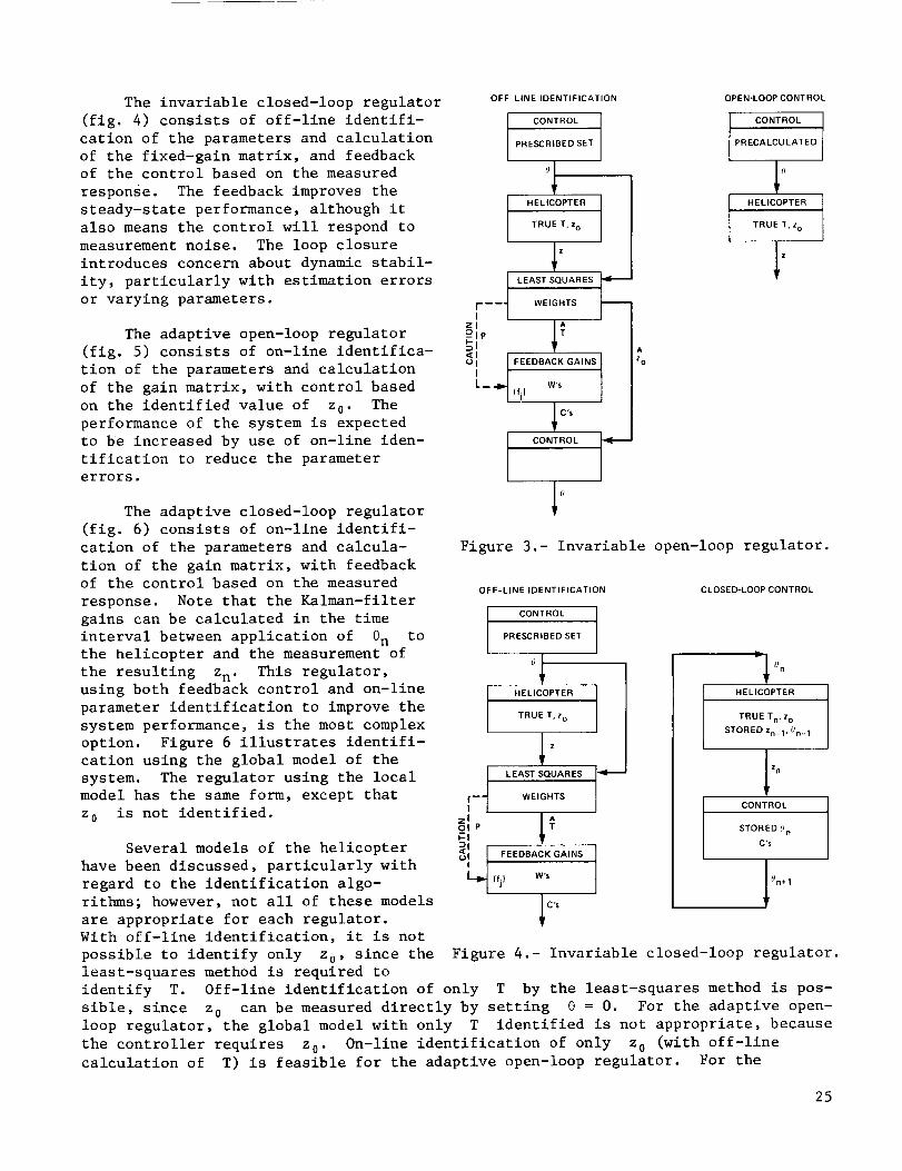
The invariable closed-loop regulator
(fig. 4) consists of off-line identifi-
cation of the parameters and calculation
of the fixed-gain matrix, and feedback
of the control based on the measured
response. The feedback improves the
steady-state performance, although it
also means the control will respond to
measurement noise. The loop closure
introduces concern about dynamic stabil-
ity, particularly with estimation errors
or varying parameters.
The adaptive open-loop regulator
(fig. 5) consists of on-line identifica-
tion of the parameters and calculation
of the gain matrix, with control based
on the identified value of z0. The
performance of the system is expected
to be increased by use of on-line iden-
tification to reduce the parameter
errors.
The adaptive closed-loop regulator
(fig. 6) consists of on-line identifi-
cation of the parameters and calcula-
tion of the gain matrix, with feedbackof the control based on the measured
response. Note that the Kalman-filter
gains can be calculated in the time
interval between application of en to
the helicopter and the measurement of
the resulting zn. This regulator,
using both feedback control and on-line
parameter identification to improve the
system performance, is the most complex
option. Figure 6 illustrates identifi-
cation using the global model of the
system. The regulator using the local
model has the same form, except that
z 0 is not identified.
Several models of the helicopter
have been discussed, particularly with
regard to the identification algo-
rithms; however, not all of these models
are appropriate for each regulator.
With off-line identification, it is not
possible to identify only z U, since the
least-squares method is required to
OFF-LINE IDENTIFICATION OPEN-LOOP CONTROL
I CONTROLPRESCRIBED SET
l HELICOPTERTRUE T, z o
t LEAST SQUARESI- -- -- WEIGHTS
I
_" Ito I FEEDBACK GAINS
I
L_ (fi) W's
II C's
I CONTROL
I CONTROL 1PRECALCULATED
TRUE T, z o
A
z o
Figure 3.- Invariable open-loop regulator.
OFF-LINE IDENTIFICATION
I CONTROLPRESCRIBED SET
I HELICOPTERTRUE T, z o
t LEAST SQUARES-- WEIGHTS
oIP
_ FEEDBACK GAINS(fj) W's
C's
CLOSED-LOOP CONTROL
l HELICOPTER
TRUE Tn, z o
STORED Zn_ 1. Un-1
z n
CONTROL
STORED 0 n
C's
Figure 4.- Invariable closed-loop regulator.
identify T. Off-line identification of only T by the least-squares method is pos-
sible, since z 0 can be measured directly by setting e = 0. For the adaptive open-
loop regulator, the global model with only T identified is not appropriate, because
the controller requires z 0. On-line identification of only z0 (with off-line
calculation of T) is feasible for the adaptive open-loop regulator. For the
25

OPEN-LOOP CONTROL
_Ylf_n
HELICOPTER
TRUE Tn, Zon
STORED Zn_l, _n-1
I z n
ON-LINEIDENTIFICATION adaptive closed-loop regulator, on-line
identification of only T (with off-line
calculation of z0) is possible. TheKALMANGAINS global model with on-line identification
I of only z0 is not appropriate for theSTOREDMnORPn-1 adaptive closed-loop regulator, since the
On'rn system then reduces to the invariable
kn I
A
CONTROL FEEDBACK GAINS
STORED _)n
t}n+ 1
M I
n+l I
Figure 5.- Adaptive open-loop regulator.
CLOSED-LOOP CONTROL
HELICOPTER
TRUE T n, Zon
STORED Zn_l, 0n_ 1
z n
ON-LINE IDENTIFICATION
KALMAN GAINS l
STORED M n OR Pn-1
Qn, rn
closed-loop option. Finally, the local
model is not appropriate with off-line
identification, and it cannot be used for
the adaptive open-loop regulator (which
requires z0).
In summary, the global model with
identification of both z 0 and T can be
used with all four regulator options.
Identifying only T is possible for all
options, except the adaptive open-loop
(z0 must still be estimated, of course,
by direct measurement for the invariable
options or by off-line identification for
the adaptive option). On-line identifica-
rIP kn_
I KALMAN FILTERSTOR ED ZAOn_l, "?'n_l
CONTROL FEEDBACK GAINS
STORED (_n
tion of only z 0 can be used for the
adaptive open-loop regulator, and the
local model can be used for the adaptive
closed-loop regulator.
Previous Work
Previous work has been reported on
the application of each of these four
regulator options. Table 1 summarizes
these investigations (see also the discus-
)n+l
w's (fj)
I
I
I
I
Mn+ll
Figure 6.- Adaptive closed-loop regulator.
sion of previous work in the Introduc-
tion). The work has been both experimen-tal and theoretical. The identification
techniques considered include the off-line
least-squares method; recursive estimation
by a Kalman filter; and direct inversion
of the measured data (when the number of
independent control inputs equals the num-
ber of controls). The controller gains
have been determined by (I) minimizing a
quadratic performance function, sometimes
with weights on the measurements and con-
straints on the control; (2) minimizing
the expected value of the performance
function (the cautious controller); and
(3) by direct inversion of the T-matrix
(when the number of measurements equals
the number of control variables).
The invariable open-loop regulator has received the most attention. Although
these investigations have been based primarily on experimental data, there has been
26

ZO
F_
<H
>
ZOH
_q
>
[-4
0__)
[.=1
0
O9
0
rD
ZO
O
O
I
,-1
[-..t
OZ
-H
cM ,--i i--4
II II,!J
<1 <1
o° o o
r--t 1-1 _ I-I _ I-I U O
N
rj N N N N N tJ t.J tJ _ tJ N N
II II II II II I-I I_ _ _ I_ II II• 1-1 "1-1 "1-I "H "H
0.H
t_0.1-1
g
o
[--i _O) t./)
0 "_ "_/ _ 0 ._ _ o_ _) _ _ r_ 0 0 m r_ _ I_
;_ _ :m ;m _ i::: El I_ i= _ .,4 .__ _ o- _r ..4 ._ .,_ '-_ q_
_O _ r_ r_ _ _ _ 0
r_ ,-i
0
_J
-H .rl - _-, -H .H -I-I _ -H _ "i-I -;.-I
> N N ,=: N N N N N N ,-_ N N
o
O
O _ 0 0 _
_ _ 0 0 _ _ 0
_ • _ 0
_-_ 0
0
0,_ ,--_ 0 0
> 0
_ 0 _ _
>
II g
09
>
[-_O0
.H
[_ E-_
m m0 0
0 0
0_J
• r-I ,_
!!M M
0 00 •
F_ F_
0ooO_
v
0
_o0
_v
m •
_ _2uO O
m _ [--I
0..,
00
,---4;>
0
O
¢J-H
-H
g)
.IJO
4J
,zn
e
O
>
O.H
O
¢1
O
27

no experimental confirmation of the regulator performance when the open-loop control
is applied. The open-loop control required has been calculated using the measured
T-matrix, and the response resulting when this control is applied has been predicted.
The investigations have considered blade loads (McCloud and Kretz, 1974; Kretz et al.,
1973a,b; McCloud, 1975; McCloud and Weisbrich, 1978), hub reactions (McCloud, 1975;
Sissingh and Donham, 1974; Powers, 1978; Wood, Powers, and Hammond, 1980), and
accelerations (McCloud and Weisbrich, 1978; Brown and McCloud, 1980).
There has been both experimental and theoretical work on the invariable closed-
loop regulator, including some direct experimental verification (Shaw and Albion,
1980). The vibration was successfully nulled at one speed, but not at higher or
lower speeds, because the control authority was exceeded. The transient characteris-
tics of the controller were good.
The performance of the adaptive open-loop regulator has been tested in terms of
its starting response, ability to track speed variations, and behavior with collective
changes (Molusis et al., 1981). There has been partially successful experimental
verification of the vibration reduction using this regulator (Hammond, 1980; Molusis
et al., 1981). Three quantities were controlled, using the three swashplate inputs,
but only two were significantly reduced; the roll moment (Hammond, 1980) or lateral
acceleration (Molusis et al., 1981) was only slightly reduced, or was even increased.
Molusis et al. (1981) considered six controllers in the adaptive open-loop class:
deterministic, cautious, and dual forms with both T and z0 identified; and a deter-
ministic form with only z 0 identified, including perturbation and proportional-
integral feedback variants. In their terminology, the first three controllers were
called adaptive and the last three were called gain-scheduled (since the gains dependonly on T). The perturbation variant should be identical to the basic controller
with only z0 identified, since the T-matrix perturbation was not included in the
controller-gain calculation. The cautious controller was most satisfactory, achieving
the minimum vibration within a few iterations after starting, with smooth control
variations and no indication of drift in steady conditions. The controller tracked
well with velocity changes. The deterministic controller was more erratic in opera-
tion; introduction of a rate limit produced smooth control variations, but the system
was then considered too sluggish. The regulators with only z 0 being identified were
not successful in reducing the vibration (it was conjectured that the failure was due
to nonlinearity in the T-matrix).
The performance of the adaptive closed-loop regulator has been examined in terms
of the starting response (Taylor et al., 1980) and the response to abrupt changes in
the parameters (Shaw, 1980). There has been no experimental verification of this
regulator. Only the local model has been considered. Taylor et al. (1980) found that
a limit on the maximum control increment was needed for smooth operation (I_e I < 0.i °
in a single step, for each harmonic). They also examined the influence of the time-
step and measurement noise on the system performance. An update interval of two
revolutions produced somewhat smoother response, but the system converged faster with
a one revolution increment. With a measurement noise level above 20% of the uncon-
trolled response, the regulator did not converge. Taylor et al. (1980) actually
identified Zn_ I as well as T, which leads to inconsistencies. They considered thehelicopter model in the form
ZnZnliCn)28

Henceat the (n - 1)th step, Zn_I was a measurement;at the nth step, Zn_I becamea parameter. Furthermore, the model of the parameter variation used with the Kalmanfilter gives Zn_I = Zn_2 + Uzn_2, which is not consistent with the helicopter model,Zn_I = Zn_2 + T(0n_I - @n_2).
ANALYSISANDSIMULATION
The regulators that have been defined in the preceding sections must be analyzedin more detail, in order to further develop useful designs for helicopter vibrationalleviation. Of concern regarding the on-line identification are the transientbehavior and convergence; identifiability; and the selection of the parameters in thealgorithm. Of concern for the controller are the interpretation and selection of theweights in the performance function; the possible use of cautious or dual controllers;and the stability and steady-state performance of the controlled system, includingthe effects of measurementnoise, parameter-estimation errors, and nonlinear or time-varying parameters. Someof these issues will be examinedhere by considering asystem with only one measurementand one control. The actual helicopter probleminvolves sine and cosine componentsfor each harmonic, and usually at least threeharmonics or variables for the input and output. The single-input and single-outputcase is useful however, because of the simplifications that result from dealing withscalar equations. The identification proceeds by rows in fact, so with a singleinput there actually is a scalar equation in the identification algorithm for eachmeasurement. The weighting matrix Wz then is used to balance the control of thevarious output variables (the specific influence of Wz depends on the elements ofT). For the general multi-input and multi-output case, it is necessary to dealdirectly with the matrix equation given above.
The characteristics of the regulators will be analyzed in the following sectionsby examining the equations for the case of a system with only one measurementand onecontrol. In addition, numerical simulations were performed for several of the cases.The general behavior exhibited in the numerical simulations will be described,although it is not considered appropriate to present quantitative results from simu-lations of such a simple system.
Open-LoopControl
For open-loop control, involving feedback of the uncontrolled vibration level,the deterministic controller is
8n = C_0 + C&eSn_I = (-TWz_0 + WAeSn_l)/(@ZWz + We + WAe)
With a single output, Wz is not relevant; it is retained however, to aid in theinterpretation of the parameters for the multivariate case. For the invariable open-loop regulator, WA0 must be zero; for the adaptive open-loop regulator, T and Zo arethe estimates at the (n - l)th step. The stability of this controller is determinedby the eigenvalue
+We + )x = wAs/(@2wz wAe
29

The corresponding time-constant is
T = At%/(l - %) = AtWA@/(T2W z + We)
so the time lag is directly proportional to WAe/T2Wz .
W 0 , but
T/At _ WAO
0ss/-_0 _2wz
The time lag is reduced by
where ess is the steady-state response (given below). So the rate limit, which is
proportional to 0ss/m, is independent of W 0.
The steady-state limit of the controller is
en = -TWzZ01(T2Wz + We)
(which is reached immediately if WA@ = 0). Now define _0 as the solution of
z = z 0 + Te = 0, and let T o = T at 0= e 0. Similarly, 0 o is the solution of the
equation using the estimated parameters, z = z0 + Te = 0; hence 00 -z0/T. Then
the steady-state control is
el60 = 11(I + wel@2wz)
and the system response is
z/zo = (i - T_o/@Zo + Wol#2Wz)l(1 + Wel#2Wz)
The response in the presence of parameter errors depends on both T and 20, which may
have either canceling or reinforcing effects. Hence, it is clearer to write the
response in terms of the error in the estimate of 00:
zlz0 = (i - Te01r000 + Wel#2Wz)/(l + wel#2Wz)
With no estimation errors, the result is
zlz0 = (WelT2Wz)/(l + We/T2Wz) = i - e/S0
Note that a feedback control law of the form 0 = -Kz gives z/z 0 = i/(i + KT), which
implies KT = T2Wz/W0. Thus, W e may be interpreted as the inverse of the gain.
Closed-Loop Control
For closed-loop control, involving feedback of the measured vibration, the
deterministic controller is
= C e 8nen Cz + (I-)n-I -i
+ ]l(_2w + w e + WAO)= [-TWzZn-i + (@2Wz WAe)On-I z
30

where T is the estimate at the (n - l)th step. To examine the closed-loop perfor-
mance, substitute Zn_ I = z 0 + Ten_ I + Vn_ I, to obtain
8 1 {__WzZ 0 + [T(T - T)W z + WAO]8 n i - TWzVn-l}n _ _
where
A = T2W + W e +z WAe
It is assumed that the parameters vary slowly enough to be considered constant for the
present purposes. Nonlinear behavior of the real system will be allowed however, so
T = T(On_l). Note there are no dynamics in the helicopter model, since the quasi-static assumption gives a model of the form zn = f(On). The dynamics are introduced
by the control law. An equation for the response is obtained by substituting
On = (zn - z0)/T in the controller equation, and including the measurement noise in
Zn_ I. For a linear system the result is
i ^ ^ - TTWvZn = _ {Wez0 + [T(T - T)W z + WAe]Zn_ I z n-l
Here z is the true response of the system, without the measurement noise.
For the ideal case, a linear system with no estimation errors, these equations
reduce to
e 1n = 7 (-TWzZ0 + WAeen_ I - TWzVn_ I)
iz = + - T2W v )n _ (Wezo WAoZn-I z n-I
The eigenvalue is
+w o + )= WAo/(T2W z WA@
and the steady-state solution is
e/e o = i/(i + Wo/T2W z)
z/z o = (We/T2Wz)/(l +We/T2W z)
If the system starts with e 1 = O, then z I = z 0 and
= z /(T2W +W e +WAe)ez -TWz o z
= + W e + WAe)z2 zo(W e + WAO)/(T2W z
It is observed that the eigenvalue is the same as in the open-loop case. The time lag
is again determined by WAe. This ideal system is always stable (Ill < i). The
steady-state solution is also the same as that for the open-loop case (for no estima-
tion errors); hence, the interpretation of W 0 is the same. If WAe = O, the
31

steady-state solution is reached immediately (at n = 2). The steady-state response
to the measurement noise is
o_Ir = (TWzlA)21[I - (wAelA)Z ]
= (TWz)Z/[(T2W z + We)(TzW z + W 8 + 2WAe)]
2and dz = Toe" Here o_ and o z are the mean-squared responses of en and zn to the
noise v n, which is a Gaussian random variable with zero mean and variance E(v 2) = r.
These results can be written
= + /(T2W + W e + 2W&o)(°_/02)/(r/z_) (r2Wz We) z
(o_Iz_)l(rlz_) = (el00)2(T2W z + Wg)I(T2W z + We + 2wAe)
which are both order one. The rate limit WAe reduces the response to measurement
noise.
For a linear system with estimation errors, the eigenvalue is
^ ^
- +W e ÷k = [T(T T)W z + WA@]I(T2W z WA0 )
= (I - T/_ + wAe/_2Wz)/[1 + (we + wAe)/_2Wz]
For stability, Ikl < I, it is thus necessary that
-We/T2W z < T/T < 2 + (W e + 2WAe)/T2Wz
If W e = WAe = 0, the criterion is that 0 < T/T < 2; that is, the estimated value of
T must have the same sign and at least 50% the magnitude of the true value. It is
found that this result is unchanged by the addition of the steady-state Kalman-filter
dynamics. The control constraints W 8 and WA8 improve the stability range. The
steady-state solution is now
0 = (-z_/T)/(1 + W0/TTWz)
z = z0(W0/TTWz)/(I + W0/TTWz)
So with feedback of Zn_ I, the steady-state response is not sensitive to estimation
errors, except for a c_ange in the influence of W e . Specifically, with W e = 0, the
null response z = 0 is always achieved. Feedback of the measured vibration intro-
duces a response to measurement noise however, and estimation errors do influence the
system stability. The stability range is large, but on-line identification is still
likely to be required for the helicopter problem.
For a nonlinear system, T(Sn_l) must be used in the equation for On . The
steady-state solution is still given by the above equations. Now an explicit equa-
tion for the control is not possible, since T depends on e; but still, z = 0 is
achieved if W e = 0. Convergence and stability of the nonlinear equation for e n
are difficult to examine analytically, but the local stability can be calculated.
32

Consider the nonlinear equation en = a + b(0n_1)en_1, and a solution On of this
equation for the specified initial conditions. For a perturbation about this solu-
tion, On = en + _8n, the linearized equation is
_en = (b + 0 _b/_O)6en_ I
where the coefficient is evaluated at O = en_ I. Hence the eigenvalue is
i
% = b + @b' = 7 [_(_ - T - @T')Wz" + WAol.
for the present problem, and the stability criterion becomes
-W@/T2W < (T + @T')/T < 2 + (W@ + 2WAo)/T2Wz z
So the estimate T must be close to T + @T', which is just the local slope of the
response z(@).
Caution and Learning
Accounting for uncertain parameters in the performance function has the effect
for open-loop control of replacing W@ with (W@ + %cMttWz ), and introducing theoffset
c o = -% DM Wc tz z
if z 0 is identified. For the cautious controller, %c = i. The open-loop controlalgorithm than becomes
8n = (-TWz _0 - MtzWz + WAeOn-i )/(_2Wz + We + WA8 + MttWz)
which has the steady-state solution
8/_ 0 = (I + Mtz/T_0)/(l + Ws/T2W z + Mtt/T2 )
z
z 0
i - (T00/T0O0)(l + Mtz/T_0) + We/T2W z + Mtt/T2
1 + Wo/T2W z + Mtt/T2
With parameter errors there is a shift in the control required to obtain the minimum
expected value of J. The control is always decreased by an error in T, while Mtz
can produce a control change in either direction.
For closed-loop control, WAS is replaced by (WA8 + kcMttWz), where again %c = 1for the cautious controller. The control algorithm becomes
8 = [-TW z + (T2W + + ]/(T2W + W@ + + Mn z n-1 z WA@ MttWz)en-1 z WA8 ttWz )
The steady-state solution is not influenced by the caution in this case, but the
response to measurement noise will be decreased and the stability range increased.
33

The effectiveness of the caution is determined by the normalized squared errors,
Mtt/T 2 and Mzt/_ 0. For example, an rms error of 20% gives Mtt/T 2 = 0.04, which
would produce only small changes in e and z. To have a significant influence of the
caution, Mtt/T 2 must be order one, which implies an extremely large estimation error.
It is probable that the regulator performance would be unacceptable with such large
errors. The recursive identification algorithm is often started with extremely large
values of P0 (typically P0/T 2 & I0). The caution would then be active at the start
and would have the effect of limiting or smoothing the control until the parameters
are estimated well. However, W e or WAS could be used instead, with the same effect.
Also, the identifiability problem with a closed-loop system can lead to large estima-
tion errors for individual parameters, which would be reflected in large values of
the error variance P (although P/T 2 could still be small). The caution could
become effective in this case.
Recall that a form of learning controller can be obtained by using %c < 0. The
control diverges at _cMtt/T 2 = -i (if W 0 = WAS = 0). For the learning to be effec-
tive however, the magnitude of %cMtt/T 2 must be order one. Hence this learning
controller operates near the divergence, and with a much reduced stability range for
the closed-loop control. These characteristics make this type of dual controller
unacceptable.
Adaptive Identification
To examine the characteristics of the recursive parameter identification, con-
sider the algorithm for the identification of T in the global helicopter model:
= T + k - z 0 - T en)n n-I n(Zn n-I
where
m = +n Pn- i qn- 1
Pn I = m-ln + 0n2/rn ' or Pn = mnrn/(rn + mn n02)
k n = Pnen/rn = mnen/(r n + mnSZn)
The generalized least-squares solution is obtained by setting q = 0:
n n
Pn-' = p-ln_1 + 0n/rn = p_l + _ 0_/r i __ E 02/r ii=l i=l
en/r nk =n n
E 8Z/riii=l
2For the least-squares case, r n = constant; therefore, k n = 0n/Z8 i approaches zero as
n increases. This algorithm is not appropriate for recursive identification because
it shuts off. As data are acquired, each new piece of information is worth less and
less compared with the accumulated knowledge. In contrast, by using the exponential
34
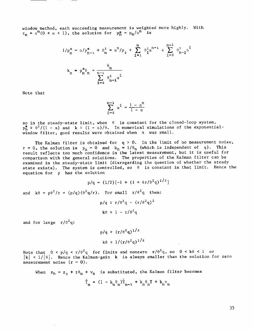
window method, each succeeding measurement is weighted more highly. With
rn = _n(o < _ < I), the solution for p_ = pn/_ n is
n n-i
i/Pn, , 02 n _z n-1= _/Pn-I + = _ /P0 + Eni=i i=0
k = pn*On n
en
n-I2 i
en_i_i=0
Note that
n-I n
E ai = i- _1 -
i=O
so in the steady-state limit, when e is constant for the closed-loop system,
p_ m 0Z/(l - _) and k _ (i - _)/e. In numerical simulations of the exponential-
window filter, good results were obtained when _ was small.
The Kalman filter is obtained for q > 0. In the limit of no measurement noise,
r = 0, the solution is Pn = 0 and k n = I/e n (which is independent of q). This
result reflects too much confidence in the latest measurement, but it is useful for
comparison with the general solutions. The properties of the Kalman filter can be
examined in the steady-state limit (disregarding the question of whether the steady
state exists). The system is controlled, so e is constant in that limit. Hence the
equation for p has the solution
p/q = (1/2)[-1 + (I + 4r/e2q) I/z]
and ke = pe2/r = (p/q)(e2q/r). For small r/e2q then:
p/q m r/e2q - (r/62q) 2
ke m 1 - r/e2q
and for large r/02q:
Note that 0 < p/q < r/e2q for finite and nonzero r/e2q, so 0 < ke < i or
Jk I < 1/le I . Hence the Kalman-gain k is always smaller than the solution for zero
measurement noise (r = 0).
When zn = z 0 + te n + v n is substituted, the Kalman filter becomes
= (I - knen)T + k _ T + k vn n-I nn nn
35

The dynamics of this equation will be examinedseparately, although in fact the filterand controller form a coupled system. Note that in general (i - knen) = Pn/mn, whichis positive and less than i. In the steady-state limit, kn_n is constant, so thefilter equation is time-invariant with eigenvalue %= i - k0. Recall 0 < ke < i,so 0 < _ < i; the filter is stable. For small r/e2q
-" r/82q m 0
and for large r/O2q
% m 1 - 1/(r/e2q) I/2 _ i
Now % m 0 implies immediate convergence, _n = T; and % _ i implies no convergence
at all, Tn = Tn-1" Hence a large value of q is better than a large value of r.
The limit q/r = 0 is the least-squares algorithm, so the tracking ability will be
poor for large r/e2q. The converged solution of the filter is T = T, unless _ = i
exactly. The filter response to the measurement noise is
o_/q = (r/82q)/(l + 4r/@2q) I/2
The mean-square response of the identified parameter, _, is large for large values
of r/O2q.
In general, the solution for small values of e = r/82q is
pn/qn_l _ i/(I + 8_qn_i/rn) + 0(s 3)
rn/8_qn_ I + 0(e 2)
So p/q is order _ small always. This result gives the steady-state solution and
the limit r = 0 properly too. If the solution is started with i/Po = 0, then
Pl = rl/8_" So Pn immediately has the order required for the small r/82qsolution.
The general solution for large values of r/82q is
Pn/qn-I m (Pn-I/qn-I + i) - (enqn_12 /rn)(Pn_i/qn_l + i)2 + 0(_3e2)
where _ = p/q and e = 82q/r. This equation is valid only if I_ I < g-l, that is,
if p/q i_ smaller than order e-1. Indeed, this equation eventually gives p/q
order c -I/2, which is the proper steady-state solution also. If p/q is order
_-i, however, the solution to lowest order is
qn_i/Pn _ qn_i/Pn_l + 0_qn_i/r n + 0(7 -2 )
Again, i/Po m 0 gives Pl = rl/Sz I" So this order e-I solution is encountered at
the start of the algorithm, and whenever p/q becomes too large. If the order _-I
solution proceeds for N steps, then
qn_I/pn = _ e2qi_I/r i -_ N e
N steps
36

So eventually p/q becomes smaller than order ¢-i, and the order C-I/2 solution
is encountered. The number of steps that the solution remains order s-1 is
inversely proportional to s. In the limit e = 0, the order c-I solution is
always valid; in fact, the equation above is the exact solution for g = qO2/r = 0
(namely, the least-squares limit).
For the global model, it is anticipated that
@2q/r = (@2/e_)(q/T2)/(r/z_)
will be order one for typical values of q and r. For the identification of
corresponding parameter
qir= (qJ4)J(riz )
z 0, the
should also be order one. With the local model however, "O" is interpreted as A@,
and
Ae_q/r = (Ae21e_)(q IT2)l(rtz2)o _ (Ae/eo)2
will be small. Hence, difficulties may be anticipated with identification of the
local model. In numerical simulations of this case, the estimate of the local T
diverged in the presence of measurement noise (the filter shuts off without measure-
ment noise). The controlled response remained acceptable however. The system was
stable because the estimate of T was greater than the true value. The divergence of
the estimate was not eliminated by the use of WAO, a large value of q, a limit on
the minimum magnitude of AO, or caution. The estimate did not diverge when T
varied with time, although the tracking ability of the filter was not as good as when
the global model was used.
Identifiability
When both z0 and T are identified, the Kalman filter is
= [i - k@ n(:on)1- k JVon_U n
In the steady state, where O and the Kalman gains are constants, the eigenvalues of
this equation are X = i and X = i - k z - k0, with corresponding eigenvector matrix
As discussed above, the k = 1 eigenvalue reflects the problem of identifying two
parameters with one measurement for a closed-loop system. In numerical simulations of
the above equations, the identified parameters diverged in the presence of measurement
noise, with _0 + T0 remaining near the correct value. The estimated value of T
was large, so the controller was stable, and the controlled response remained accept-
able. The use of WA@ or caution did not improve the identifiability. The estimates
37

did not diverge when the parameters varied with time, although the undamped(z0 + Te)modewas still evident.
Someof the phenomenaencountered by Molusis et al. (1981) in tests of an adap-tive open-loop regulator are consistent with the use of a cautious controller in thecontext of the identifiability problems with a closed-loop system. They were identi-fying 42 parameters, using six measurements,so a large parameter variance P wouldbe expected in steady-state conditions. Direct evidence of the identifiability prob-lem is provided by the fact the T-matrix obtained by on-line identification was notthe sameas that obtained by off-line identification, and by the observation that theT-matrix identified on-line was not repeatable. A large value of P would make thecaution effective, which is consistent with the fact that the cautious controller wassmoother than the deterministic controller, and with the observation that the weight-ing matrix Wz influenced the solution (Hammond,1980) (those are the influencesof the effective control weight We due to caution). That the roll momentorlateral acceleration was not reduced could also be due to a large effective value ofWe• The observation that during speed changes the controller actually maintained thevibration below the levels obtained in steady conditions is consistent with reducedcaution resulting from improved identifiability when the parameters vary. There arehowever other factors, such as nonlinearity, that might account for someof theseeffects. The argument is also contradicted by the statement that the samestabilizedcondition was approachedwith the deterministic controller as with the cautiouscontroller (Hammond,1980).
Adaptive Open-LoopRegulator
For the combination of open-loop control and on-line identification, the coupledcontroller and filter dynamics must be considered in order to analyze the regulatorperformance. The steady-state solution (if it exists) of the Kalmanfilter is
z = zo + TG= Zo + _8
In this result, either z0 or T maybe estimated on-line, and the other parameterobtained from off-line calculations; or both maybe identified on-line. A linearsystem is assumed,but T maybe the local derivative of z(8). The Kalman-gainsinfluence the convergence of the filter, but not the steady-state solution. Usingthe open-loop control solution, the steady-state response of the regulator is then
e = [-%Wz/(_2wz + w0)][z0 + (T - #)_]
= (-zo/T)l(l + W0/T@W z)
z = zo(Ws/TTWz)/(I + We/TTWz)
which is the same as the closed-loop control result. The response depends on the
actual response z 0 rather than the estimate _0, because of the on-line identifica-
tion. Recall that the open-loop response depends on the error in e0" From
zo + T8 = zo + T8 it follows that
T/T = (Zo/Zo)(l + W0/T2Wz) - Wo/T2W z
38

zol£o = (T/@ + wel¢2Wz)/(1 + Wel_2wz)
and so
i - _oleo = I - T£01@z0 = (_01z0 - I)(We/_2Wz)
= (i - T/T)(We/T2Wz)/(T/T + W0/T2Wz)
which is zero regardless of the parameter errors if W e = 0. The filter identifies
one or both parameters such that the measured value of z will be predicted cor-
rectly. Hence the parameter errors must compensate in the vicinity of this value of
the response. With a controlled system the response will be small, so the error in
the estimate of O0 (where z = 0) should be much smaller than the error in the indi-
vidual parameter estimates. Thus the regulator has good closed-loop performance.
When only z0 is identified, the equations for the filter and controller are
Z0n = Z0n_z + k - ^ - Te)n(Zn Zon_ I
= +On CZ0n_ z CA68n_ z
This system is linear. Although kn varies with time initially, it depends only on
qn and rn, not on @n in this case. Assuming that qn and rn are constant, it is
appropriate to use the steady-state solution for kn. Substituting for
zn = z 0 + T8 n + vn gives the equations
\ nl
k(T - T)CAe l ^c0 )+
Ik(z0 0+ Vn) 1
In the ideal case, with no error in the estimate of T, the filter is decoupled from^
the controller. The estimate Z0n follows z 0 + vn (actually measured as zn - T6n)
with a first-order lag (% = i - k). Then the control 8n follows Z0n with a lag
due to WA8 (% = CA@),, and the response zn is determined by @n" The steady-state
response of the filter to the measurement noise is
o20/r = k/(2 - k)
2where °0 is the mean-squared response of _0n to the noise vn, which is aGaussian random variable with zero mean and variance E(v 2) = r. Then the mean-
squared response of the control @n is
The first factor in o_ identical to the response of the closed-loop controller to
measurement noise. The product of the last two factors is always less than i, so the
adaptive open-loop regulator has a smaller response to noise than does the closed loop
controller. The eigenvalues of the coupled system are the solutions of
39

%2_ [i - k + k(T - T)C + CA@]%+ (i - k)C&e = 0
If T = T, the filter and controller are decoupled and the solutions are %= i - kand %= CAe. In general, the criterion for stability (1%1< i) is
-W0/T2Wz < T/T < 1 + [(2 - k)/k][1 + (W@+ 2W4@)/T2Wz]
If W@= WAO= 0, the system is stable if 0 < T/T < 2/k. Since k < i, the stabilityrange is larger than for the closed-loop controller.
In numerical simulations of the adaptive open-loop regulator, good performancewas obtained when only z0 was identified, although the ability to handle a systemwith a time-varying value of T was not very good. In wind-tunnel tests however,Molusis et al. (1981) found that the regulator using identification of z0 only wasnot successful in reducing the vibration.
CONCLUSIONS
Self-tuning regulators for the multicyclic control of helicopter vibration havebeen examined. The topics considered have included the selection of the parametersfor the identification and control algorithms; the best combination of identification,control, and helicopter model options for the regulator; and the regulator perfor-mance, involving steady-state response, stability, convergence, and identifiability.
Regarding the identification algorithms, it is concluded that the values of theparameter variance and measurementnoise variance must be correctly chosen for properperformance of the regulators. The use of the Kalman filter is preferred to theexponential-weighted generalized least squares, since the former is more flexible andthe theory provides a guide for the choice of the parameters.
Regarding the controller algorithms, the analysis has provided guidelines forthe choice of the parameters. The use of the largest value of WA@that does notmakethe response too sluggish is appropriate, to improve the transient response, thesensitivity to measurementnoise, and the sensitivity of the stability to parametererrors. The rate limit WA@should always be used during the start of the recursiveidentification, and a small value of WA@can be used to avoid the possibility ofcontrol divergence, should the estimated T-matrix be too small. The control magni-tude constraint W8 maynot be too useful, since it limits the control relative tothe ideal value O0 rather than relative to an absolute value. Absolute limits onthe control magnitude are probably better applied by uniformly reducing the elementsof @ before the commandsignals are sent to the actuators. The benefits of thecautious controller can probably be obtained more directly by the appropriate choicesof W@and WA@(which could be temporarily increased in special circumstances such asthe start of the identification algorithm). The use of a dual controller does notappear necessary, since the identifiability problems encountered are not accompaniedby poor controller performance.
Regarding the regulator algorithms, it is concluded that the following options(in order of preference based on simplicity) are potentially applicable to the controlof helicopter vibration.
40

I. Invariable open-loop regulator: This is the simplest option. It has nostability problems. This regulator will be satisfactory only if there are no signif-icant parameter errors.
2. Invariable closed-loop regulator: This option provides good performance ifthe measurementnoise is not too large. It will be satisfactory if the parameters donot vary so much that the system becomesunstable.
3. Adaptive open-loop regulator, with only the uncontrolled vibration levelidentified: This is the simplest adaptive option. It has no identifiability prob-lems, and mayprovide good performance and stability. This regulator will be satis-factory if it can provide good control, particularly with time-varying parameters.
4. Adaptive open-loop or closed-loop regulator, with all parameters identified:This option probably has the best performance with time-varying parameters. The open-loop and closed-loop cases are nearly indistinguishable in terms of system perfor-mance. This regulator will be satisfactory if the identifiability problems do notdegrade the performance, and if the helicopter response is not too nonlinear.
5. Adaptive closed-loop regulator, with the local helicopter model: This optionis probably most suitable for very nonlinear systems; however, there are identifiabil-ity problems.
The theoretical and experimental work to date concerning these regulators sug-gests that an adaptive system will be needed. Hence, it is anticipated that one ofthe last three options will be required for helicopter vibration control.
RECOMMENDATIONS
Further work on self-tuning regulators for the multicyclic control of helicoptervibration is required in the following topics.
i. The conclusions of the present report must be verified or modified for themultivariable case. The implications of the use of cosine and sine componentsin theinput and measurementsmust be investigated.
2. Techniques for the numerical implementation of the identification and controlalgorithms must be developed.
3. The regulator development can be extended; for example, dynamics can beincluded in the helicopter model, and dual controllers could be considered further.
4. The regulator designs must be examinedmore thoroughly in terms of the spe-cific characteristics of the helicopter, including the selection of the control andmeasurementvariables; off-design performance or the performance with time-varyingparameters; the influence of noise and nonlinearities; and the influence of theregulator on the helicopter trim and on the stability augmentation system.
41

Finally, the regulators require further experimental development and experimen-tal confirmation of their performance in order to complete the development.
AmesResearch CenterNational Aeronautics and SpaceAdministration
Moffett Field, California 94035, September21, 1981
42
REFERENCES
Anderson, Brian D. 0.; and Moore, John B.: Optimal Filtering. Prentice-Hall,EnglewoodCliffs, N.Y., 1979.
Astrom, K. J.; Borisson, U.; Ljung, L.; and Wittenmark, B.: Theory and Applicationsof Self-Tuning Regulators. Automatica, vol. 13, no. 5, 1977, pp. 457-476.
Astrom, K. J.; and Wittenmark, B.: On Self-Tuning Regulators. Automatica, vol. 9,no. 2, 1973, pp. 185-199.
Brown, T. J.; and McCloud, J. L., III: Multicyclic Control of a Helicopter RotorConsidering the Influence of Vibration, Loads, and Control Motion. AnnualForumof the American Helicopter Society, Washington, D.C., May 1980.
Bryson, Arthur E., Jr.; and Ho, Yu.-Chi.: Applied Optimal Control: Optimization,Estimation and Control. Blaisdell Publishing Company,Waltham, Mass. 1969.
Gelb, Arthur, ed.: Applied Optimal Estimation. The MIT Press, Cambridge, Mass.,1974.
Goodwin, GrahamClifford; and Payne, Robert L.: Dynamic SystemIdentification:Experiment Design and Data Analysis. AcademicPress, NewYork, 1977.
Hammond,C. E.: Wind Tunnel Results ShowingRotor Vibratory Loads Reduction UsingHigher Harmonic Blade Pitch. 21st Structures, Structural Dynamics, andMaterials Conference, AIAA, Seattle, Wash., 1980.
Johnson, Wayne: Helicopter Theory. Princeton University Press, Princeton,NewJersey, 1980.
Kretz, M.; Aubrun, J.-N.; and Larche, M.: Wind Tunnel Tests of the Dorand DH 2011Jet Flap Rotor. Vol. I. NASACR-I14693, 1973a.
Kretz, M.; Aubrun, J.-N.; and Larche, M.: Wind Tunnel Tests of the Dorand DH 2011Jet Flap Rotor. Vol. 2. NASACR-I14694, 1973b.
McCloud, J. L., III: An Analytical Study of a Multicyclic Controllable Twist Rotor.Paper No. 932, 31st Annual Forumof the American Helicopter Society, Washington,D.C., May 1975.
McCloud, J. L., III: The Promise of Multicyclic Control for Helicopter VibrationReduction. Vertica, vol. 4, no. I, 1980a.
McCloud, J. L., III: Multicyclic Control for Helicopters: Research in Progress atAmesResearch Center. 21st Structures, Structural Dynamics, and MaterialsConference, AIAA, Seattle, Wash., 1980b, pp. 77-81.
McCloud, J. L., III; and Kretz, M.: Multicyclic Jet-Flap Control for Alleviation ofHelicopter Blade Stresses and Fuselage Vibration. Rotorcraft Dynamics, NASASP-352, 1974, pp. 233-238.
43
McCloud, J. L., III; and Weisbrich, A. L.: Wind Tunnel Test Results of a Full-ScaleMulticyclic Controllable Twist Rotor. Paper No. 78-60, Annual Forumof theAmerican Helicopter Society, Washington, D.C., May 1978.
McHugh,F. J.; and Shaw,J., Jr.: Helicopter Vibration Reduction with Higher HarmonicBlade Pitch. J. American Helicopter Soc., vol. 23, no. 4, 1978, pp. 26-35.
Mendel, Jerry M.: Discrete Techniques of Parameter Estimation: The Equation ErrorFormulation. Marcel Dekker, Inc., NewYork, 1973.
Molusis, J. A.; Hammond,C. E.; and Cline, J. H.: A Unified Approach to the OptimalDesign of Adaptive and Gain Scheduled Controllers to Achieve MinimumHelicopterRotor Vibration. 37th Annual Forumof the American Helicopter Society,NewOrleans, La., May 1981.
Powers, R. W.: Application of Higher Harmonic Blade Feathering for Helicopter Vibra-tion Reduction. NASACR-158985,1978.
Sage, AndrewP.; and Melsa, JamesL.: Estimation Theory with Applications to Com-munications and Control. McGrawHill Book Company,NewYork, 1971.
Shaw, John: Higher Harmonic Blade Pitch Control: A Systemfor Helicopter VibrationReduction. Ph.D. Thesis, Massachusetts Institute of Technology, May 1980.
Shaw, J.; and Albion, N.: Active Control of the Helicopter Rotor for VibrationReduction. Paper No. 80-68, 36th Annual Forumof the American HelicopterSociety, Washington, D.C., 1980.
Sissingh, G. J.; and Donham,R. E.: Hingeless Rotor Theory and Experiment on Vibra-tion Reduction by Periodic Variation of Conventional Control. RotorcraftDynamics, NASASP-352, 1974, pp. 261-277.
Taylor, R. B.; Farrar, F. A.; and Miao, W.: An Active Control Systemfor HelicopterVibration Reduction by Higher Harmonic Pitch. Paper No. 80-71, 36th AnnualForumof the American Helicopter Society, Washington, D.C., May 13-15, 1980.
Taylor, R. B.; Zwicke, P. E.; Gold, P.; and Miao, W.: Analytical Design and Evalua-tion of an Active Control System for Helicopter Vibration Reduction and GustResponseAlleviation. NASACR-152377, 1980.
Wittenmark, B.: Stochastic Adaptive Control Methods: A Survey. Int. J. Control,vol. 21, no. 5, 1975, pp. 705-730.
Wood, E. R.; Powers, R. W.; and Hammond,C. E.: OnMethods for Application of Har-monic Control. Vertica, vol. 4, no. I, 1980.
44


1 Report No, 2. Government Accession No. 3. Recipient's Catalog No.
NASA TP-1996
4. Title and Subtitle
SELF-TUNING REGULATORS FOR MULTICYCLIC CONTROL
OF HELICOPTER VIBRATION
7, Author(s)
Wayne Johnson
9. Performing Organization Name and Addre_
Ames Research Center, NASA
Moffett Field, Calif. 94035
12. Sponsoring Agency Name and Address
National Aeronautics and Space Administration
Washington, D.C. 20546
5. Re_rt Date
March 1982
6. Performing Organization Code
8. Performing Organization Re_rt No.
A-8719
10. Work Unit No.
505-42-21
11, Contract or Grant No.
13, Type of Report and Period Covered
Technical Paper
14. Sponsoring Agency Code
15, Supplementary Notes
Point of contact: Wayne Johnson, Ames Research Center, 247-i,
Moffett Field, CA 94035, (415)965-5043 or FTS 448-5043
16. Abstract
A class of algorithms for the multicyclic control of helicopter
vibration and loads is derived and discussed. This class is characterized
by a linear, quasi-static, frequency-domain model of the helicopter
response to control; identification of the helicopter model by least-
squared-error or Kalman-filter methods; and a minimum variance or quad-
ratic performance function controller. Previous research on such con-
trollers is reviewed and related to the present work. The derivations
and discussions cover the helicopter model; the identification problem,
including both off-line and on-line (recursive) algorithms; the control
problem, including both open-loop and closed-loop feedback; and the
various regulator configurations possible within this class. Conclusions
from analysis and numerical simulations of the regulators provide guidance
in the design and selection of algorithms for further development, includ-
ing wind-tunnel and flight tests.
17. Key Words (Suggested by Author(s))
Helicopter
Vibration control
Self-tuning regulator
18. Distribution Statement
Unclassified - Unlimited
Subject Category 08
19. Security Classif, (of this report)
Unclassified
*For sale by the NationaITechnic_I Information Service, Springfield, Virginia 22161
20 Security Classif. (of this _ga}
Unclassified
21. No. of Pa_s 22. Dice"
51 A04
NASA-Langl ey, 1982