+Lab 4: Expert Groups 008

Group

1 David Guillermo Lauren Mallory

2 Jonathon Vivian Kristen

3 Alexander B

Berkley Melanie Eddie

4 Richard Keltan Heather Skriba

5 Chris Maya Heather Smallwood

Alexander W

6 Mollie Brad Hannah

7 Erin Howie Anna Pujiao

8 Jessica Elliot DominicPlease sit with your group and do not log on the computers.

+Lab 4: Expert Groups (010)

Group

1 Brad So Yun Kris Molly

2 Jacob Alex Peter

3 Drake Danny Derek Andrew

4 Ashley Michelle Emily R

5 Emily F Matt Matan Grant

6 Madeline Renee Taylor

7 Katie Mardie Chrissy Gordon

8 Emily J Joseph Supriya

Please sit with your group and do not log on the computers.

+

STATS 250 Lab 3

Julie GhekasSeptember 22, 2014

Please don’t log in. We will not be using the computers, and we will be moving.

+Schedule

Lab 2 Wrap Up

Probability

Warm Up

Lab 3

Cool Down/iClicker Questions

Example Exam Question

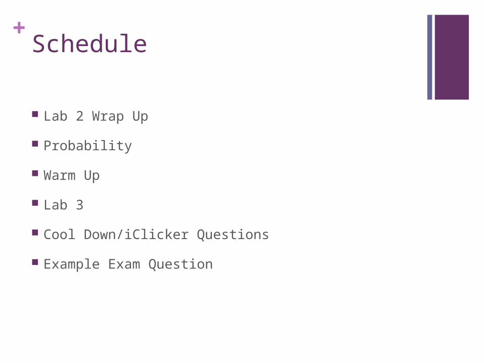
+Practice Homework Comments

Only 80% of you turned in homework

As a class, you struggled the most with Q3

Estimating the percent of time over 90 minutes Show work Count frequencies over 90/total (272) *100

Graph Describe the shape In context With values

+Time Plots

Looks can be misleading Has a time variable on the x-axis

Checking for stability to check independently distributed assumption Trend means no trend, no seasonal variation, and no

pattern in variation

Should make histogram only when the time plot shows stability

+Lab 2: Time-Dependent Data

1949

1952

1955

1958

1961

1964

1967

1970

1973

1976

1979

1982

1985

1988

1991

1994

1997

2000

2003

2006

2009

2012

0

50

100

150

200

250

300

350

400

Average Yards Earned by UM fb

rush yards/gamepass yards/game

Season

Avera

ge G

am

e Y

ard

age

+Lab 2: Time-Dependent Data

1 3 5 7 9 11 13 15 17 19 21 23 25 27 29 31 33 35 37 39 41 43 45 470

50

100

150

200

250

300

Pass yards by Game 1981-1984

Sequence Number

Overa

ll p

ass y

ard

s/g

am

e

+QQ Plots

Is the sample drawn from a normally distributed population?

We want a roughly straight line.

Remember that we are making inferences about the population.

Shows the relationship between quantiles (Q) of observed data and quantiles (Q) of expected of a normal distribution.

+Ticket: Warm Up Answers

+Ticket: Cool Down Answers

+Ticket: Cool Down Answers

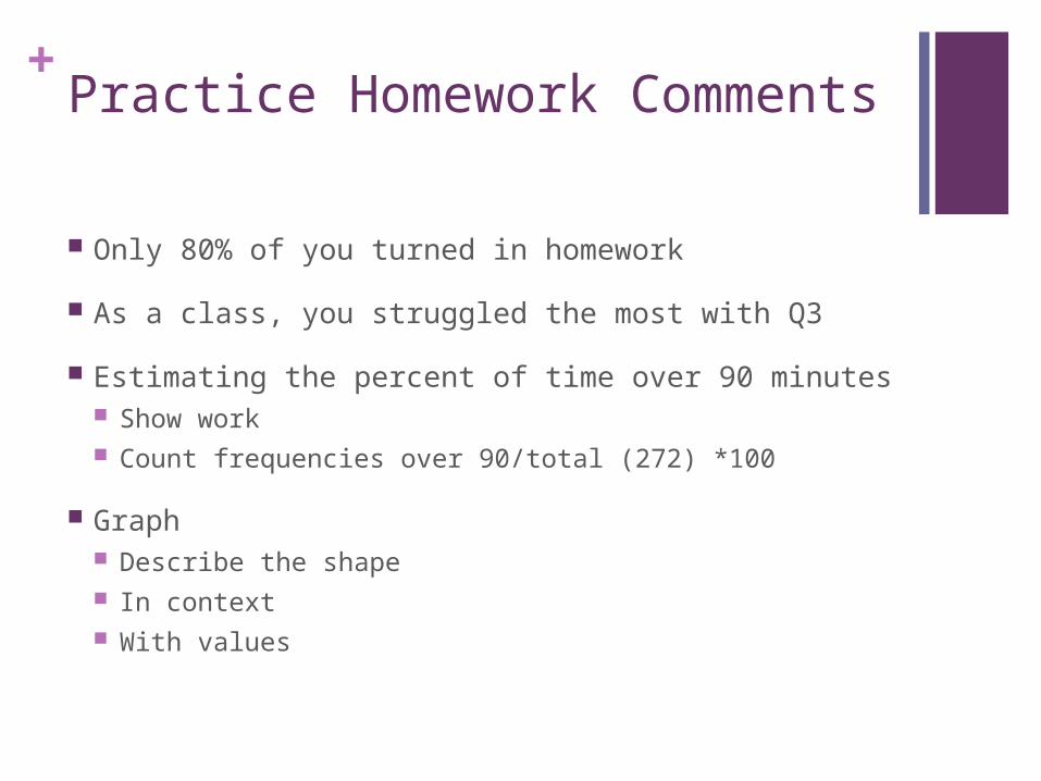
+Probability

+Probability

Three distributions that you have learned: Normal X~N(μ, σ)

Standard Normal X~N(0, 1) Binomial X~Binom(n, p)

Normal Approximation for Binomial Distribution Uniform X~Unif(a,b)

Two probability definitions that you have learned: Independent events Mutually exclusive events

+Probability

Rules from Yellow Formula Card

To calculate the probability of an observation by hand: Draw distribution curve Shade appropriate area of the curve Calculate the probability using z-table if normal distribution Calculate area under the curve if continuous random

variable Add the individual probabilities if discrete random variable

+Probability Calculations

Empirical rule can answer some probability questions

What if empirical rule fails because observation is not exactly on a standard deviation from the mean?

Example: random variable IQ scores for Americans IQ~N(100,20) P(IQ>125) Draw the curve, and shade the area Find the z-score, and use Table A1 on your formula card

+Probability Calculations: Table A1

Use only with Normal distributions

Provides probabilities for a standard normal curve

Gives area to the left of a z-score

Let’s try using Table A1

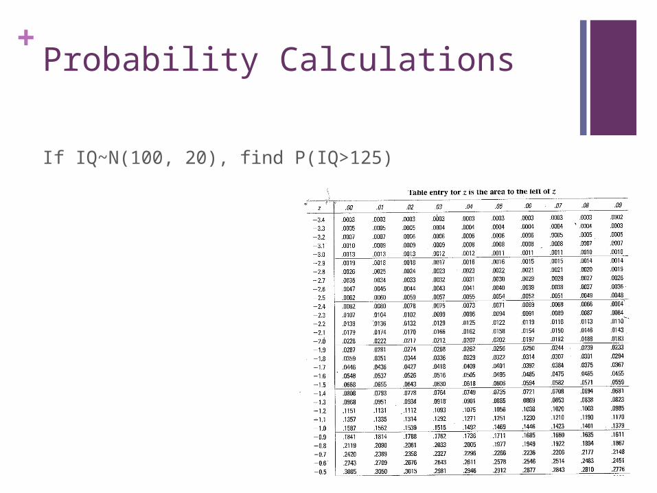
+Probability Calculations

If IQ~N(100, 20), find P(IQ>125)

+Probability Calculations

Can use R to calculate probability

Canvas -> R Tutorials -> Probabilities in R -> Download file under Necessary Files header

Open the downloaded prob-calc.rdata

Type prob( ) to start the program

Type q to quit

Calculate P(Z<1.2)

+Probability Calculations

Can use R to calculate probability

Canvas -> R Tutorials -> Probabilities in R -> Download file under Necessary Files header

Open the downloaded prob-calc.rdata

Type prob( ) to start the program

Type q to quit

Calculate P(Z<1.2) = 0.8849

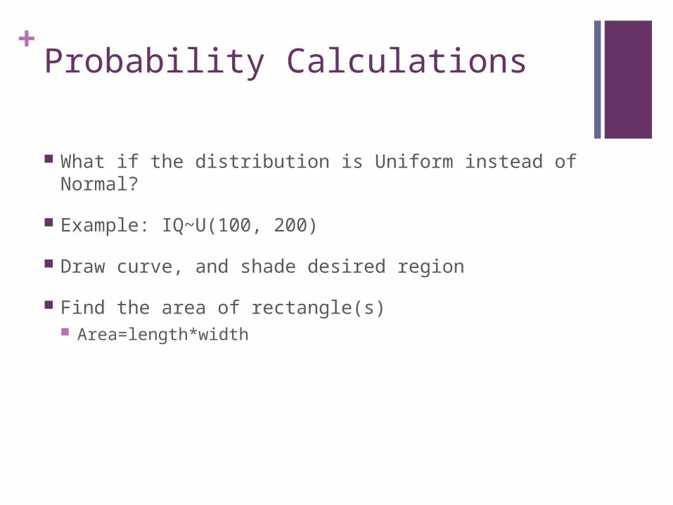
+Probability Calculations

What if the distribution is Uniform instead of Normal?

Example: IQ~U(100, 200)

Draw curve, and shade desired region

Find the area of rectangle(s) Area=length*width

+Probability Calculations

If IQ~U(100, 200), find P(IQ>125)

+Probability Calculations

If discrete random variable, then sum up all of the individual probabilities

Binomial distribution is a discrete distribution Binomial counts the number of successful trials with equal

probability p if you perform n trials

Consider flipping a coin 10 times. If X is a random variable for the number of heads, X~Bin(10, 0.5), assuming the coin is fair

+Probability Calculations

If X~ Bin(10, 0.25), find P(X<2)

+Warm Up

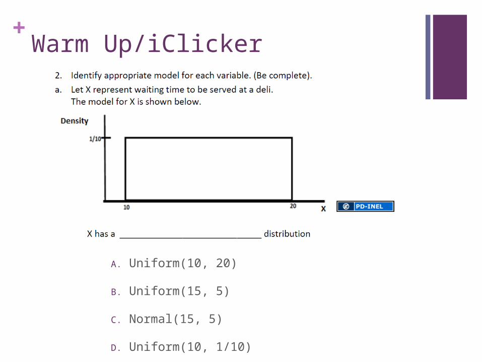
+Warm Up/iClicker

A. Uniform(10, 20)

B. Uniform(15, 5)

C. Normal(15, 5)

D. Uniform(10, 1/10)

+Warm Up/iClicker

A. Uniform(10, 20)

B. Uniform(15, 5)

C. Normal(15, 5)

D. Uniform(10, 1/10)

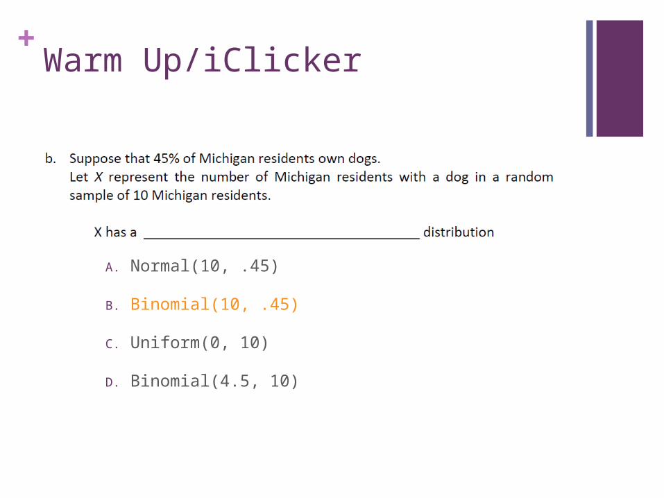
+Warm Up/iClicker

A. Normal(10, .45)

B. Binomial(10, .45)

C. Uniform(0, 10)

D. Binomial(4.5, 10)

+Warm Up/iClicker

A. Normal(10, .45)

B. Binomial(10, .45)

C. Uniform(0, 10)

D. Binomial(4.5, 10)

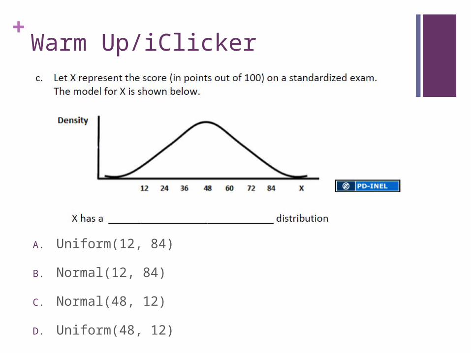
+Warm Up/iClicker

A. Uniform(12, 84)

B. Normal(12, 84)

C. Normal(48, 12)

D. Uniform(48, 12)

+Warm Up/iClicker

A. Uniform(12, 84)

B. Normal(12, 84)

C. Normal(48, 12)

D. Uniform(48, 12)

+Lab 4: Expert Groups 008

Group Problem Float

1 1 David Guillermo Lauren Mallory

2 1 Jonathon Vivian Kristen

3 2 Alexander B

Berkley Melanie Eddie

4 2 Richard Keltan Heather Skriba

5 3 Chris Maya Heather Smallwood

Alexander W

6 3 Mollie Brad Hannah

7 4 Erin Howie Anna Pujiao

8 4 Jessica Elliot DominicDon’t worry about the R-script part of Problem 4

Change Question 3 part c to “Interpret the z-score.”

+Lab 4: Expert Groups (010)

Group Problem Float

1 1 Brad So Yun Kris Molly

2 1 Jacob Alex Peter

3 2 Drake Danny Derek Andrew

4 2 Ashley Michelle Emily R

5 3 Emily F Matt Matan Grant

6 3 Madeline Renee Taylor

7 4 Katie Mardie Chrissy Gordon

8 4 Emily J Joseph Supriya

Don’t worry about the R-script part of Problem 4

Change Question 3 part c to “Interpret the z-score.”

+Lab 4: Share Groups 008

Problem 1 2 3 4

1 David Alexander B Chris Erin

2 Guillermo Berkley Maya Howie

3 Lauren Melanie Heather Smallwood

Anna

4 Jonathon Richard Mollie Pujiao

5 Vivian Keltan Brad Jessica

6 Kristen Heather Skriba

Hannah Elliot

7 Mallory Eddie Alexander W Dominic

Don’t worry about the R-script part of Problem 4

+Lab 4: Share Groups (010)

Problem 1 2 3 4

1 Brad Drake Emily F Katie

2 So Yun Danny Matt Mardie

3 Kris Derek Matan Chrissy

4 Molly Andrew Grant Gordon

5 Jacob Ashley Madeline Emily J

6 Alex Michelle Renee Joseph

7 Peter Emily R Taylor Supriya

Don’t worry about the R-script part of Problem 4

+Lab 4: Problem 1

a. What is the probability that a randomly selected person smiled?

b. To check if smiling status is independent of gender, (a) should be compared to:P(smiled and male) P(smiled given male)P(male given smiled) P(male)

c. Find (b).

d. Do smiling status and gender appear to be independent?

Smile No Smile Total

1=Male 3269 3806 7075

2=Female 4471 4278 8749

Total 7740 8084 15824

+Lab 4: Problem 2

Suppose the probability of 7 days is twice as likely as the probability of 8 days. Complete the probability distribution.

What is the expected number of days for the longest trip? Include symbol, value, and units.

X 4 5 6 7 8

Probability 0.10 0.20 0.25

+Lab 4: Problem 3

Which are correct? On average, the number of hours spent studying

statistics varied from the mean by about 3.5 hours. The average distance between the number of hours

spent studying statistics is roughly 3.5 hours. The average number of hours spent studying statistics

is about 3.5 hours away from the mean.

+Lab 4: Problem 3

Assume the mean is 10 and the standard deviation is 3.5. Julie studies for about 6 hrs/week. What is her z-score?

Male students have a lower mean and larger standard deviation than female students. Jake’s response corresponds to z=2.1. Can we compare scores?

+Lab 4: Problem 4

Assume that for Chem, the mean is 12 and the standard deviation is 3.

What is the probability that a randomly selected Chemistry student studies between 16 and 20 hours per week?

+Lab 4: Problem 4

Assume that for Chem, the mean is 12 and the standard deviation is 3.

Jing learns that she is in the top 30%. This means that Jing must study at least how many hours per week?

+Cool Down/iClicker

If the time to wait for pharmacy help has a uniform distribution from 0 to 30 minutes, then 33% of the customers are expected to wait for more than 20 minutes.

A. True

B. False

+Cool Down/iClicker

If the time to wait for pharmacy help has a uniform distribution from 0 to 30 minutes, then 33% of the customers are expected to wait for more than 20 minutes.

A. True

B. False

+Cool Down/iClicker

If X has a Binomial(50, 0.7) distribution, then the criteria to use the normal approximation are met.

A. True

B. False

+Cool Down/iClicker

If X has a Binomial(50, 0.7) distribution, then the criteria to use the normal approximation are met.

A. True

B. False

+Cool Down/iClicker

68% of all test scores will fall within one standard deviation of the mean test score.

A. True

B. False

+Cool Down/iClicker

68% of all test scores will fall within one standard deviation of the mean test score.

A. True

B. False

+Cool Down/iClicker

Police report that 78% of drivers stopped on suspicion of drunk driving are given a breath test, 36% are given a blood test, and 22% are given both tests. Do the police administer these two tests independently?

A. True

B. False

+Cool Down/iClicker

Police report that 78% of drivers stopped on suspicion of drunk driving are given a breath test, 36% are given a blood test, and 22% are given both tests. Do the police administer these two tests independently?

A. True

B. False

+iClicker

If the variable X is strongly skewed to the right with a mean of 80 and a standard deviation of 2, then 95% of the values are expected to be between 76 and 84.

A. True

B. False

+iClicker

If the variable X is strongly skewed to the right with a mean of 80 and a standard deviation of 2, then 95% of the values are expected to be between 76 and 84.

A. True

B. False

+iClicker

Suppose the amount spent by students on materials for summer half term has approx a normal, bell-shaped distribution. Mean amount spent was $300 and standard deviation was $100.

About 68% of the students spent between ____.

A. $300 and $400

B. $200 and $400

C. $100 and $500

D. $266 and $334

+iClicker

Suppose the amount spent by students on materials for summer half term has approx a normal, bell-shaped distribution. Mean amount spent was $300 and standard deviation was $100.

About 68% of the students spent between ____.

A. $300 and $400

B. $200 and $400

C. $100 and $500

D. $266 and $334

+iClicker

Suppose the amount spent by students on materials for summer half term has approx a normal, bell-shaped distribution. Mean amount spent was $300 and standard deviation was $100.

What amount spent on materials has a standardized score of 0.5?

A. $150

B. $250

C. $300.50

D. $350

+iClicker

Suppose the amount spent by students on materials for summer half term has approx a normal, bell-shaped distribution. Mean amount spent was $300 and standard deviation was $100.

What amount spent on materials has a standardized score of 0.5?

A. $150

B. $250

C. $300.50

D. $350

+iClicker

Suppose the amount spent by students on materials for summer half term has approx a normal, bell-shaped distribution. Mean amount spent was $300 and standard deviation was $100.

Approx what percent of students spent more than $400 on materials?

A. 16%

B. 32%

C. 68%

D. 50%

+iClicker

Suppose the amount spent by students on materials for summer half term has approx a normal, bell-shaped distribution. Mean amount spent was $300 and standard deviation was $100.

Approx what percent of students spent more than $400 on materials?

A. 16%

B. 32%

C. 68%

D. 50%

+Example Exam Question

+Example Exam Question

What is P(A)?

What is P(A and B)?

What is P(B|A)

What is P(A and C)?

Are the events A and C mutually exclusive?

+iClicker

How did you feel about the material covered in today’s lab?

A. Completely understood everything

B. Understood main ideas, shaky on details

C. Good for the first half, lost for the second

D. Trouble with some main ideas

E. Difficulty following most material

+Reminders

Homework 1 is open and due Thursday at 8 am

No prelab due this week

Can do prelab for next week