Data-Adaptive Estimation and Inference inthe Analysis of Differential Methylation

for the annual retreat of the Center for Computational Biology,given 18 November 2017

Nima HejaziDivision of Biostatistics

University of California, Berkeleystat.berkeley.edu/~nhejazi

nimahejazi.orgtwitter/@nshejazi

github/nhejazi

slides: goo.gl/xabp3Q

This slide deck is for a brief (about 15-minute) talk on a newstatistical algorithm for using nonparametric and data-adaptiveestimates of variable importance measures for differential methylationanalysis. This talk was most recently given at the annual retreat ofthe Center for Computational Biology at the University of California,Berkeley.

Source: https://github.com/nhejazi/talk_methyvimSlides: https://goo.gl/JDhSEgWith notes: https://goo.gl/xabp3Q

Preview: Summary▶ DNA methylation data is extremely high-dimensional

— we can collect data on 850K genomic sites withmodern arrays!

▶ Normalization and QC are critical components ofproperly analyzing modern DNA methylation data.There are many choices of technique.

▶ A relative scarcity of techniques for estimation andinference exists — analyses are often limited to thegeneral linear model.

▶ Statistical causal inference provides an avenue foranswering richer scientific questions, especially whencombined with modern advances in machine learning.

1

We’ll go over this summary again at the end of the talk. Hopefully, itwill all make more sense then.

Motivation: Let’s meet the data

▶ Observational study of the impact of disease state onDNA methylation.

▶ Phenotype-level quantities: 216 subjects, binarydisease status (FASD) of each subject, backgroundinfo on subjects (e.g., sex, age).

▶ Genomic-level quantities: ∼ 850, 000 CpG sitesinterrogated using the Infinium MethylationEPICBeadChip by Illumina.

▶ Questions: How do disease status and differentialmethylation relate? Is a coherent biomarker-typesignature detectable?

2

• FASD is an abbreviation for Fetal Alcohol Spectrum Disorders.

• We’re mostly interested in the interplay between disease andDNA methylation.

• In particular, we’d like to construct some kind of importancescore for CpG sites impacted by the exposure/disease of interest.

• Re: dimensionality, c.f., RNA-seq analyses are ∼ 30, 000 indimension at the gene level.

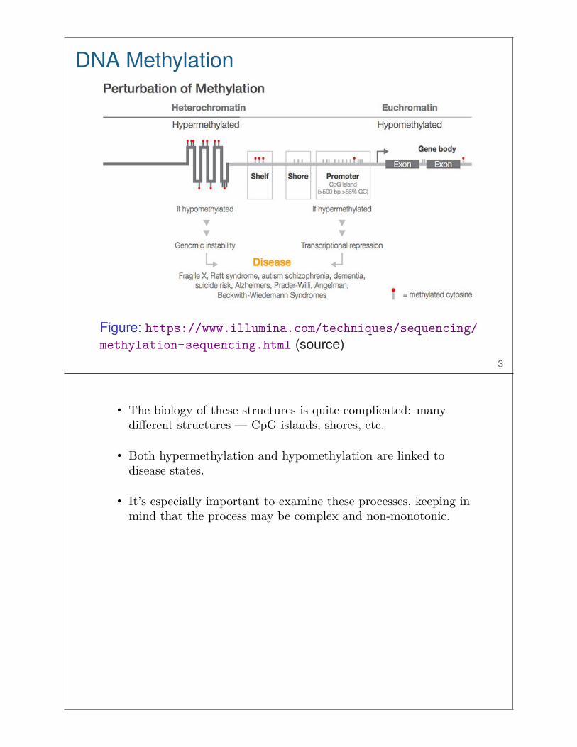
DNA Methylation

Figure: https://www.illumina.com/techniques/sequencing/methylation-sequencing.html (source)

3

• The biology of these structures is quite complicated: manydifferent structures — CpG islands, shores, etc.

• Both hypermethylation and hypomethylation are linked todisease states.

• It’s especially important to examine these processes, keeping inmind that the process may be complex and non-monotonic.

Data analysis? Linear Models!▶ Standard operating procedure: For each CpG site

(g = 1, . . . , G), fit a linear model:

E[yg] = Xβg

▶ Test the coefficent of interest using a standard t-test:

tg =β̂g − βg,H0

sg

▶ Such models are a matter of convenience: does β̂ganswer our scientific questions? Perhaps not.

▶ Is consideration being given to whether the data couldhave been generated by a linear model? Perhaps not.

4

• CpG sites are thought to function in networks. Treating them asacting independently is not faithful to the underlying biology.

• The linear model is a great starting point for analyses whne thedata is generated using complex technology — no need to makethe analysis more complicated.

• That being said, the data is difficult and expensive to collect, sowhy restrict the scope of the questions we’d like to ask.

Motivation: Science Before Statistics

What is the effect of disease statuson DNA methylation at a specific CpGsite , controlling for the observedmethylation status of the neighborsof the given CpG site?

5

• Again, CpG sites are thought to function in networks. Treatingthem as acting independently is not faithful to the underlyingbiology.

• This means that we should take into account the methylationstatus of neighboring CpG sites when assessing differentialmethylation at a single site.

• This is a coherent scientific question that we can set out toanswer statistically. It’s motivated by the established scienceand possible to do with modern statistical methodology.

Data analysis? A Data-Adaptive Approach

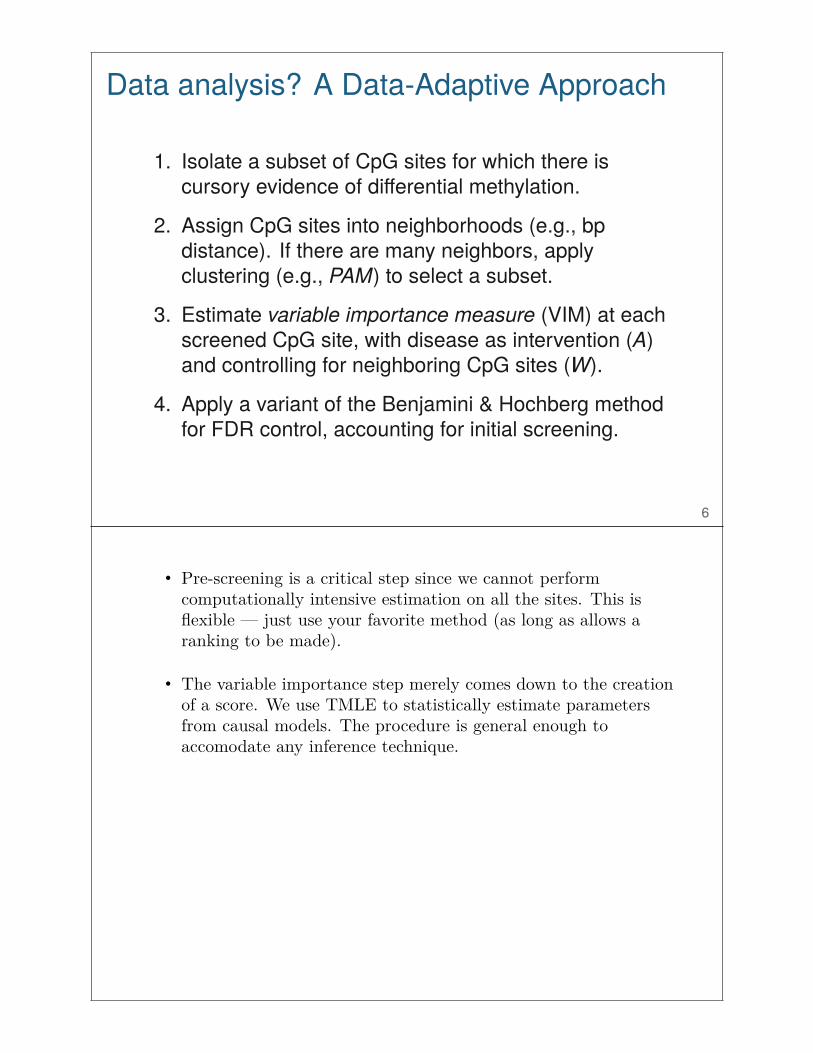
1. Isolate a subset of CpG sites for which there iscursory evidence of differential methylation.

2. Assign CpG sites into neighborhoods (e.g., bpdistance). If there are many neighbors, applyclustering (e.g., PAM) to select a subset.

3. Estimate variable importance measure (VIM) at eachscreened CpG site, with disease as intervention (A)and controlling for neighboring CpG sites (W).

4. Apply a variant of the Benjamini & Hochberg methodfor FDR control, accounting for initial screening.

6

• Pre-screening is a critical step since we cannot performcomputationally intensive estimation on all the sites. This isflexible — just use your favorite method (as long as allows aranking to be made).

• The variable importance step merely comes down to the creationof a score. We use TMLE to statistically estimate parametersfrom causal models. The procedure is general enough toaccomodate any inference technique.

Pre-Screening — Pick Your Favorite Method

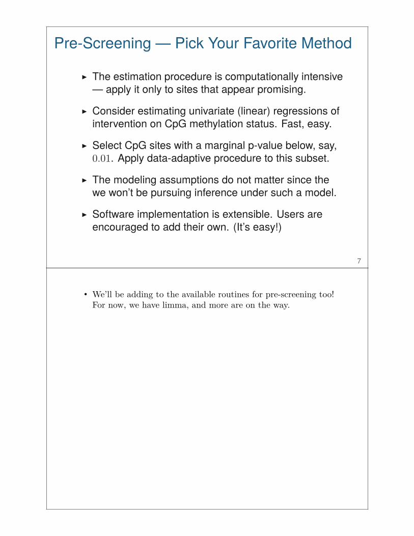
▶ The estimation procedure is computationally intensive— apply it only to sites that appear promising.

▶ Consider estimating univariate (linear) regressions ofintervention on CpG methylation status. Fast, easy.

▶ Select CpG sites with a marginal p-value below, say,0.01. Apply data-adaptive procedure to this subset.

▶ The modeling assumptions do not matter since thewe won’t be pursuing inference under such a model.

▶ Software implementation is extensible. Users areencouraged to add their own. (It’s easy!)

7

• We’ll be adding to the available routines for pre-screening too!For now, we have limma, and more are on the way.

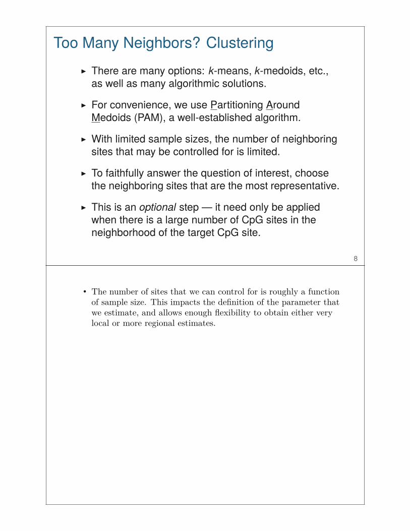
Too Many Neighbors? Clustering▶ There are many options: k-means, k-medoids, etc.,

as well as many algorithmic solutions.

▶ For convenience, we use Partitioning AroundMedoids (PAM), a well-established algorithm.

▶ With limited sample sizes, the number of neighboringsites that may be controlled for is limited.

▶ To faithfully answer the question of interest, choosethe neighboring sites that are the most representative.

▶ This is an optional step — it need only be appliedwhen there is a large number of CpG sites in theneighborhood of the target CpG site.

8

• The number of sites that we can control for is roughly a functionof sample size. This impacts the definition of the parameter thatwe estimate, and allows enough flexibility to obtain either verylocal or more regional estimates.

Nonparametric Variable Importance▶ Let’s consider a simple target parameter: the average

treatment effect (ATE):

Ψg(P0) = EW,0[E0[Yg | A = 1, W−g]−E0[Yg | A = 0, W−g]]

▶ Under certain (untestable) assumptions, interpretableas difference in methylation at site g with interventionand, possibly contrary to fact, the same under nointervention, controlling for neighboring sites.

▶ Provides a nonparametric (model-free) measure forthose CpG sites impacted by a discrete intervention.

▶ Let the choice of parameter be determined by ourscientific question of interest.

9

By allowing scientific questions to inform the parameters that wechoose to estimate, we can do a better job of actually answering thequestions of interest to our collaborators. Further, we abandon theneed to specify the functional relationship between our outcome andcovariates; moreover, we can now make use of advances in machinelearning.

Target Minimum Loss-Based Estimation▶ We use targeted minimum loss-based estimation

(TMLE), a method for inference in semiparametricinfinite-dimensional statistical models.

▶ No need to specify a functional form or assume thatwe know the true data-generating distribution.

▶ Asymptotic linearity:

Ψg(P∗n) − Ψg(P0) =

1

n

n∑

i=1

IC(Oi) + oP

(1√n

)

▶ Limiting distribution:√

n(Ψn − Ψ) → N(0, Var(D(P0)))

▶ Statistical inference:Ψn ± zα · σn√

n10

Under the additional condition that the remainder term R(P̂∗, P0)

decays as oP

(1√n

), we have that

Ψn − Ψ0 = (Pn − P0) · D(P0) + oP

(1√n

), which, by a central limit

theorem, establishes a Gaussian limiting distribution for theestimator, with variance V(D(P0)), the variance of the efficientinfluence curve (canonical gradient) when Ψ admits an asymptoticallylinear representation.

The above implies that Ψn is a√

n-consistent estimator of Ψ, that it isasymptotically normal (as given above), and that it is locally efficient.This allows us to build Wald-type confidence intervals, where σ2

n is anestimator of V(D(P0)). The estimator σ2

n may be obtained using thebootstrap or computed directly via σ2

n = 1n

∑ni=1 D2(Q̄∗

n, gn)(Oi)

Corrections for Multiple Testing

▶ Multiple testing corrections are critical. Without these,we systematically obtain misleading results.

▶ The Benjamini & Hochberg procedure for controllingthe False Discovery Rate (FDR) is a well-establishedtechnique for addressing the multiple testing issue.

▶ We use a modified BH-FDR procedure to account forthe pre-screening step of the proposed algorithm.

▶ This modified BH-FDR procedure for multi-stageanalyses (FDR-MSA) works by adding a p-value of1.0 for each site that did not pass pre-screening thenperforms BH-FDR as normal.

11

• Note that FDR = E[ V

R]

= E[ V

R | R > 0]

P(R > 0).

• BH-FDR procedure: Find k̂ = max{k : p(k) ≤ kM · α}

• FDR-MSA will only incur a loss of power if the initial screeningexcludes variables that would have been rejected by the BHprocedure when applied to the subset on which estimation wasperformed.

• BH-FDR control is a rank-based procedure, so we must assumethat the pre-screening does not disrupt the ranking with respectto the estimation subset, which is provably true for screeningprocedures of a given type.

• MSA controls type I error with any procedure that is a functionof only the type I error itself — e.g., FWER. This does not holdfor the FDR in complete generality.

Software package: R/methyvim

Figure: https://bioconductor.org/packages/methyvim

▶ Variable importance for discrete interventions.▶ Future releases will support continuous interventions.▶ Take it for a test drive!

12

• Contribute on GitHub.

• Reach out to us with questions and feature requests.

Data analysis the methyvim way

Figure: http://code.nimahejazi.org/methyvim 13

Review: Summary▶ DNA methylation data is extremely high-dimensional

— we can collect data on 850K genomic sites withmodern arrays!

▶ Normalization and QC are critical components ofproperly analyzing modern DNA methylation data.There are many choices of technique.

▶ A relative scarcity of techniques for estimation andinference exists — analyses are often limited to thegeneral linear model.

▶ Statistical causal inference provides an avenue foranswering richer scientific questions, especially whencombined with modern advances in machine learning.

14

It’s always good to include a summary.

References IBenjamini, Y. and Hochberg, Y. (1995). Controlling the

false discovery rate: a practical and powerful approachto multiple testing. Journal of the royal statistical society.Series B (Methodological), pages 289–300.

Pearl, J. (2009). Causality: Models, Reasoning, andInference. Cambridge University Press.

Smyth, G. K. (2004). Linear models and empirical bayesmethods for assessing differential expression inmicroarray experiments. Statistical Applications inGenetics and Molecular Biology, 3(1):1–25.

Smyth, G. K. (2005). LIMMA: linear models for microarraydata. In Bioinformatics and Computational BiologySolutions Using R and Bioconductor, pages 397–420.Springer Science & Business Media.

15

References II

Tuglus, C. and van der Laan, M. J. (2009). Modified FDRcontrolling procedure for multi-stage analyses.Statistical Applications in Genetics and MolecularBiology, 8(1):1–15.

van der Laan, M. J. and Rose, S. (2011). TargetedLearning: Causal Inference for Observational andExperimental Data. Springer Science & BusinessMedia.

van der Laan, M. J. and Rose, S. (2017). TargetedLearning in Data Science: Causal Inference forComplex Longitudinal Studies. Springer Science &Business Media.

16

Acknowledgments

Collaborators:Mark van der Laan University of California, BerkeleyAlan HubbardLab of Martyn SmithLab of Nina HollandRachael Phillips

Funding source:National Library of Medicine (of NIH): T32LM012417

17

Thank you.

Slides: goo.gl/JDhSEgNotes: goo.gl/xabp3QSource (repo): goo.gl/m5As73stat.berkeley.edu/~nhejazi

nimahejazi.org

twitter/@nshejazi

github/nhejazi18