Embed Size (px)
Citation preview

This file is part of the following reference:
Mitchell, James Leonard (2002) Ecology and
management of feral pigs (Sus scrofa) in rainforests. PhD
thesis, James Cook University.
Access to this file is available from:
http://eprints.jcu.edu.au/27723/
If you believe that this work constitutes a copyright infringement, please contact
[email protected] and quote http://eprints.jcu.edu.au/27723/
ResearchOnline@JCU

Ecology and Management of Feral Pigs (Sus scrota) in Rainforests.
Submitted by
James Leonard Mitchell
B. App. Se. (Rural Tech.); M. App. Se. (Biology)
February 2002
A thesis submitted for the degree of Doctor of Philosophy
Department of Zoology and Tropical Ecology
School of Tropical Biology
James Cook University (Townsville)

ii
Statement of Originality
I declare that this thesis is my own work and has not been submitted in any fonn for another
degree or diploma at any University or other institute oftertiary education. Information derived
from the published or unpublished work ofothers has been aclmowledged in the text and a list of
references is given

iii
Statement of Access
I, the undersigned, the author of this thesis, understand that James Cook University will make it
available for use within the University Library and, by other means, allow access to users in
other approved Libraries. All users consulting this thesis will have to sign the following
statement.
In consulting this thesis I agree not to copy or closely paraphrase it in whole or in part without
the written consent ofthe author; and to make proper public written acknowledgement for any
assistance which I have obtained from it.
Beyond this, I do not wish to place·any restriction on access to this thesis

IV
Abstract
The World Heritage Area (WHA) rainforests of the wet tropics region of northeast
Queensland, is regarded as natural heritage of outstanding universal value and one of the most
significant regional ecosystems in the world. The introduced feral pig (Sus serofa) have now
become established and widely distributed throughout the WHA. Feral pigs are believed to
have a severe negative impact on the conservation values of the WHA, however, very little
quantitative information on their ecological impacts or ecology is available for this region.
This study aims to obtain information on selected aspects of feral pig ecology and their
ecological impacts and to utilise this information to assist in developing management
strategies for feral pig control within the WHA.
The study was conducted near Cardwell, north Queensland, Australia (18 0 16' S, 1460 2' E)
from 1995 to 1999. Three broad macrohabitat areas were identified within the study site:
highland rainforests, rainforests / cropping ecotone and the coastal lowlands. Within each of
these areas, key microhabitats were selected to establish spatial and temporal patterns ofpig
diggings. Fenced exclosures were also established within the highland area to quantify the
ecological impacts associated with pig diggings. Seedling survival, the biomass of roots, leaf
litter and earthworms and soil moisture levels were used as ecological indicators of impact.
Radio tracking was used to detennine seasonal migration patterns, and seasonal home range
sizes. Aspects of pig biology including reproductive parameters, population dynamics,
population density and morphological models were derived from a sample of captured feral
pIgS.
Feral pig diggings were found to have spatial and temporal patterns; rainfall (soil moisture)
appeared to be the major influence on digging patterns. Pigs preferred to dig in specific
microhabitats and these digging patterns varied significantly due to seasonal influences. Most
diggings occurred in the early dry season and predominantly in moist (swamp and creek)
microhabitats where seasonally suitable soil moisture levels and associated earthworm
populations were present. A significant relationship between diggings and rainfall was found
with the majority of diggings occurring 3 to 4 months after the peak of the rainfall. The
majority of pig diggings were concentrated in only a small proportion of the total WHA, and
only minimal pig diggings were found throughout the general forest floor. The srpall area

microhabitats that were preferred by pigs experienced intense digging impacts, especially as
the soil began to dry out after the end of the wet season. The spatial pattern of diggings
appear to be correlated with the availability of suitable soil moisture levels for earthworm
populations to exist. The overall mean amount of ground disturbance by pig diggings for
each day was 0.09% of the surface area. Highland swamps recorded the ,most pig diggings
with over 80% of the swamp area dug up by pigs at some time during the 2 year study period.
The frequency of diggings occurring on transects was 23%.
The overall ecological effects of feral pig diggings were difficult to quantify. No significant
effects ofpig diggings were detected on leaf litter, root and eartllworm biomass or on soil
moisture levels. Significant correlations between earthworm biomass, seedling survival and soil
moisture levels were observed. However, there was a general trend that more seedlings
survived when protected from pig diggings. In total 5852 seedlings were monitored over a two
year study period. On average, 31 % more seedlings survived within the protected exclosures,
compared to the unprotected controls. Nine of the twelve exclosures had more seedlings
within the protected exclosures than within the unprotected" controls. A statistically significant
impact ofdiggings influencing the survival of seedling was only demonstrated in the drier
microhabitats, and could not be quantified in the moist microhabitats.
The exclosures were established specifically to examine the recovery of the ecological
variables after protection from further pig diggings. A clear trend of recovery of seedling
numbers was demonstrated when protected from pig diggings. Over the 2 year study, the
mean number of seedlings within the protected exclosures increased 7%, while the number in
the controls decreased 37%. The difference in seedling numbers between the exclosures and
controls were influenced by the recovery time. This was pronounced in the dry microhabitat
where a significant intergction (treatment x time) effect was found. Significantly more
seedlings survived inside exclosures during the last 8 months ofthe study. It was concluded
that seedling numbers will recover when protected from pig diggings.
No evidence of the hypothesised large-scale seasonal migration was found in this study. Pigs
in the lowlands and the highlands were sedentary and stayed within their defined home range
throughout the 4 year study period. The mean distance that any pig moved from the centre of
their calculated home range was 1.03 kma Pigs on the rainforest/crop ecotone have established
home ranges that vary in size due to seasonal influences.. Males tended to have a slightly

larger mean home range size (7.9 km2) then females (7.3 km2
) and both have a significantly
larger mean home range size in the dry season (7.7 km2) compared to the wet season (2.9 km2
).
The mean home range size calculated for all studied pigs was 5.5 km2• No significant
.difference in home range size was detected between the sexes.
The absence of seasonal migration movements was contrary to general community
perceptions. Most landholders within the region believed feral pigs migrated from the
highlands in the dry season to the coastal lowlands to forage on the ripening sugar cane and
banana crops, returning to the highlands in the wet season when the sugar cane is harvested.
No evidence was found in this study ;:;)rea to support this migration model. R_ather, the home
range study suggested that pigs moved greater distances and foraged further when food and
water become scarce in the dry season, thus increasing their interaction with humans. During
the wet season, feral pigs were more sedentary, thus human / pig interaction was lower. This
leads to the perception of higher pig populations in the dry season, interpreted as being due to
migration from the highland rainforests. The seasonal fluctuations of pig home range size on
the rainforest / crop boundary, coupled with the fluctuations in pig / human encounter rates is
the cause of the community perception of a seasonal migration pattern.
A sample of336 pigs was trapped during the 5 year trapping project. Most of the captured
sample (56%) were less then 12 months of age (mean age 15.3 months); less then 5% of the
population was calculated to be older than 5 years of age. Female pigs have an all year round
breeding pattern with a birth peak in January, the start of the wet season. The prevalence of
pregnancy was 41 % with 1.64 pregnancies per year; litter size in utero was 6.4. The mortality
rate in the first year of life was 51 %. Growth rates and morphological infonnation suggest
feral pigs within this rainforest region have faster growth rates and are on average heavier then
feral pigs in dry tropical regions. Morphometric models were developed that found significant
relationships between body measurements with body weight and age variables. These models
may be of value in future feral pig ecological studies. The studied pig population had the
general characteristics of a young healthy, fecund population, with a capacity to expand
rapidly. Reproductive potential is high, however high juvenile mortality counter - balances
the potential population gro\Vth. Population density in the lowland area was approximately 3.1
. km2pIgS .

Feral pigs have been identified as a major issue facing the management of the wet tropics WHA.
The implementation of a feral pig management strategy must rely on a clear understanding of the
severity of ecological impacts of pig diggings on WHA values and also the level of population
control required to protect these values. The management of feral pigs within the WHA is a
complex issue. A range of factors have to be considered in developing a strategy that takes into
account the bie-physical, economic and social issues of pig management within the WHA
regIon.
The economic impact caused by feral pigs to the agricultural industries on the WHA bOlUldary
are due mainly to pigs that pennanently reside in 'the raillJOrest / crop ecotone, and not by pigs
migrating down from the highlands. The timing and location of control strategies to reduce this
economic impact should therefore concentrate on the WHA boundary during the dry season
when pig home ranges expand into the maturing cropping systems. Environmental impacts
caused by feral pigs need to be managed on a priority basis. Management of pigs in the
inaccessible highland areas is impractical. Logistic and economic problems are insunnountable
with present control technology. Resources for pig managemen~ need to be targeted in areas
identified as having high environmental, social or economic values.
The ecology and management of feral pigs within the WHA rainforests encompasses a range of
issues. This study has highlighted and quantified some aspects of feral pig ecology and
management issues. Hopefully this thesis can be used as the basic stepping stone for future
research into developing effective management strategies.

v
TABLE OF CONTENTS
Statement of Originality
Statement ofAccess
Abstract
Table of Contents
List of Tables
List of Figures
Acknowledgements
Chapter 1. Introduction
1.1 General futroduction
1.2 Objectives of this Study
1.3 Genera~ Description ofthe Feral Pig
1.3.1 Description
1.3.2 Biology and Ecology
1.3.2.1w Dietw
1.3.2.2w Movements
1.3.2.3. Reproduction,
Iw4 Economic Impacts ofFeral Pigs
lw5 Environmental Impacts ofFeral Pigs
1.5.1. Australian Studies
1.5w2. Overseas Studies
1.5w3. Impact of Feral Pig Diggings
1.6 S~ary of Feral Pig Issues Relevant to the
Wet Tropics Region
Chapter 2. Description of Study Site and Selected Ecological Parameters
2.1 The Wet Tropics of Queensland World Heritage Area
2.2 Description of Study Site
2.2.1 Highland Area
2.2.2. Transitional Area
2.2.3 Lowland Area
Page No
ii
iii
iv
v
vi
vii
viii
1
1
1
4
5
6
6
8
10
11
12
12
14
16
18
19
19
19
20
22
22

2.3 Climate of Study Site
2.4 Ecological Parameters Chosen to Indicate Feral Pig
Ecological Impacts
2.4.1 Rainfall
2.4.2 Food Sources
2.4.2.1 Seedlings
2.4.2.2 Earthworms
2.4.2.3 Plant Roots
2.4.3 Litter
Chapter 3. Spatial and Temporal Patterns of Feral Pig Diggings
3.1 Introduction
3.2 Methods
3.2.1 Digging Transects
3.2.2 Ecological Sampling
3.2.3 Analysis
3.3 Results
3.3.1 Digging Index
3.3.2 Associations of Diggings With Rainfall Patterns
3.3.3 Frequency of Diggings
3.3.4 Total Diggings
3.3.5 Ecological Interactions With Diggings
3.4 Discussion
Chapter 4. The Impact of Feral Pig Diggings on Selected
Ecological Variables
4.1 Introduction
4.2 Methodology
4.2.1 Site
4w2.2 Exclosures
4.2.3 Sampling of Ecological Variables
4.2.3.1 Seedling Sampling
4.2.3.2 Biomass and SoilMoisture
23
25
26
26
26
27
29
30
31
31
32
32
34
35
37
37
42
45
47
-48
52
58
58
59
59
59
62
62
63
4.2.4 Analysis
4.3 Results
4.3.1 Seedlings
4.3.1.1 Alive Seedlings
4.3.1.2 Seedling Death Rate
4.3.1.3 Seedling Germinations
4.3.2 Biomass Sampling
4.3.2.1 Above Ground Biomass
4.3.2.2. Below Ground Biomass
4.3.3 Earthwonn Biomass
4.3.4. Soil Moisture
4.3.5 Interaction of Measured Ecological Variables
4.4 Discussion
64
65
65
65
68
70
71
71
73
73
76
76
78
Chapter 5. Feral Pig Movements 83
5.1 Introduction 83
5.2 Methods 84
5.2.1 Analysis of Migration Movement~ 86
5.2.2 Analysis of Seasonal Home Ranges 87
5.3 Results 90
5.3.1 Location Error 90
5.3.2 Migration Movements 90
5.3.3 Seasonal Home Range Study 95
5.4 Discussion 99
5.4.1 Migration Movements 99
5.4.2 Seasonal Home Ranges 102
Chapter 6. Demography of Feral Pigs 105
6.1 Introduction 105
6.2 Methods 106
6.2.1 Trapping Techniques 106
6.2.2 Trapping Success - Effort Assessment 106
6.2.3 Population Structure 107

6.2.4 Reproduction 107
6.2.5 Morphometric Measurement 107
6.2.6 Population Density 109
6.3 Results 110
6.3.1 Catch I Effort Assessment ofTrapping 110
6.3.2 Population Structure of all Captured Pigs 110
6.3.3 Reproductive Parameters 112
6.3.4 Morphometric Models 114
6.3.4.1. Relationship ofBody Measurements with Age 114
6.3.4.2. l?.elationship ofLive Body 1¥eight vvith Age 116
6.3.4.3. Relationship ofLive Body Weight and Body Length 118
6.3.5 Models ofAging 119
6.3.6 Estimates ofPopulation Density
6.3.7 Recapture Distances
6.4 Discussion
122
123
125
Chapter 7. General Discussion 133
7.1 Digging Patterns ofFeral Pig 134
7.2 Ecological Impacts ofFeral Pig 136
7.3 Feral Pig Biology 137
7.3.1 Home Range 138
7.3.2 Migration Movement Patterns ]39
7.3.3 Population Demography 140
7.4 Feral Pig Management Issues 143
7.5 Management Recommendations 145
7.6 Additional Research Required 148
7.7 Swnmary Conclusions 149
Bibliography 152

vi
List of Tables
Page
Table 1.1. ~stimated home range sizes, means and ranges (where given)
for male and female pigs derived from Australian and overseas
studies. 10
Table 3.1. The number and name of all strata, and the number of sites and
digging transects that were established within each of the three areas. 34
Table 3.2. The mean (%) daily digging index (DDI) for each stratum for
all sampling events within each of the three areas. 38
Table 3.3. Frequency of transects within each stratum that recorded any
digging for each sampling event, for each area. 46
Table 3.4. Mean earthworm biomass (g/m3) and soil moisture levels (%)
for each stratum within the three areas. 51
Table 4.1. Mean values of the ecological variables for exclosures and
controls for each stratum for each sampling event. 67
Table 4.2. Death rate (%) of established seedlings within the two strata. 70
Table 4.3. Correlation matrix for all measured ecological variables within
the dry and wet stratum. 77
Table 5.1. Estimated 950/0 error ellipse area (ha and s.e), bearing angle error (0) and
number (n) affix's used in error calculations for each pig. 92
Table 5.2.
Table 5.3.
Table 5.4.
Table 5.5.
Table 6.1.
Table 6.2.
Table 6.3.
Table 6.4.
Home ranges areas (km2) and movement distance from the
Harmonic Mean Centre (He) for all pigs within the three areas.
The total time of tracking (months) and number affixes
derived for each pig are also given.
Mean home range for male and female pigs (n) in the three
areas.
The mean and maximum distance (km) males and females
moved from the harmonic mean fix (He) of their home ral1ge
within the three areas.
Home range estimations (95% MCP) for male and female pigs
for the wet and dry seasons.
The effectiveness of trapping feral pigs in the highland and
lowland areas.
The number (n) of trapped male and female pigs and percent
(%) of the total captured for each age category. Pigs were aged
(months) by tooth eruption patterns.
Life table of male and female pigs less then 36 months of age.
Number surviving at each age category (fx), probability at birth
of surviving to age x (Ix), probability of dying at each age
category (dx) and mortality rate (qx) (Caughley 1977).
Fecundity schedule of breeding - age females (> 12 mths old)
in the trapped sample. The fecundity.rate (female births per
female) is calculated from the number (n) of trapped females
within each age category.
93
95
95
96
110
111
111
113

Table 6.5. Mean body measurements (cm) for all trapped pigs.
Significance of one-way ANOVA tests of independence of
male and female values is also given. 114
Table 6.6. Regression models of the relationship of individual body
measurements with age for all males and females pigs in the
trapped sample. 114
Table 6.7. Mean live weight (kg) for each age category of trapped male
::lnrl fpm::llp nto<:: 116_ ....- .... _ ........._ ... - r ... e:>..... •
Table 6.8. Frequency of captures. 122
Table 6.9. The estimated pig population within the study area calculated
by three capture frequency distribution estimations. 122
Table 6.10. Distances (kIn) and times (months) between recapture for all
ear tagged pigs in the lowland area. 124

vii
List of Figures
Page
Figure 2.1. Map of Study Site Showing the Three Treatment Areas 21
Figure 2.2. The mean monthly maximum and minimum temperatures (oC)
and rainfall (nun) for Cardwell (125 year average). 24
Figure 2.3. Recorded monthly rainfall (mm) for 1997 - 1998, for the three
t"'I+"....1'1:7 n ...£'Iol"'lt"'l ".c;:)LUUy aJ.~a~. k,J
Figure 3.1. Mean daily digging index (and s.e.) of each stratum over all
sampling events for the (a) Highland Area, (b) Transitional
Area and (c) Lowland Area. 39"
Figure 3.2. Temporal variations in the mean daily digging index for each
stratum within the three areas. 41
Figure 3.3. Relationship of (a) mean digging index (for all strata) within
the three areas and (b) recorded rainfall (nun). 42
Figure 3.4. The mean stratum digging index for the combined sampling
events categorised into the seasons 43
Figure 3.5. The relationship of digging index (for each stratum within each
area) to monthly rainfall lagged 1 to 8 months previously. Plot
of the calculated R2 values for the relationship of the DDI in
each stratum with each lagged (by month) rainfall event. 44
Figure 3.6. Frequency of occurrence (and s.e.) of diggings occurring on.
transects within each strata for the three areas for all sampling
events. 45

Figure 3.7. Seasonal trends in digging frequency for the means (s.e) of all
strata within each area.
Figure 3.8. Total diggings for each stratum within each area. The mean
percentage (and s.e) of transect increments that were disturbed
by pig diggings at any time over the total sampling period.
Figure 3.9. Temporal trends in earthworm biomass for each stratum, within
each area.
47
48
50
Figure 3.10. Temporal trends in soil moisture levels (%) for each stratum,
within the three areas. 51
Figure 4.1. Temporal trends in the mean number (and s.e) of seedlings
within the exclosures and matched controls, for each sampling
event in the dry and wet strata. 68
Figure 4.2. Percentage (and s.e.) of monitored seedlings mortality in the
exclosures and controls for the wet and dry strata for each
sampling event. 69
Figure 4.3. Number of seedlings germinated with the exclosures and
controls for the wet and dry strata for all sampling events. 71
Figure 4.4. Mean (and s.e.) of above ground biomass in each sampling
event for the exclosures and controls within the dry and wet
stratum. 72
Figure 4,,5. Mean (and s.e) of below ground biomass (g) for all exclosures
and controls within the dry and wet strata. 74
Figure 4.6. Mean (and s.e) of earthworm biomass (g) for exclosures and
controls within the dry and wet strata. 75

Figure 4.7. Mean (and s.e) soil moisture content (%) for all exclosures and
controls within the dry and wet strata. 76
Figure 5.1. Map of KeIll1edy Valley used for seasonal home range area
study.
Figure 5.2. Home range outlines for all pigs used in the migration
movement study.
Figure 5.3. R_elationship of home range ::lrea ::lnd number of location fixes
u~ed to derive the home range estimate. Regression line is
shown.
Figure 5.4. Mean home range size (km2 and s.e.) of male and females pigs
within the wet and dry season, and the aggregate home range
for both seasons combined.
89
91
94
97
Figure 5.5. Home range outlines for all pigs used in the seasonal home
range study. 98
Figure 6.1. The number (n) of trapped male and females pigs (less then 36
months of age) that were born in each month of the year
estimated from backdating age at capture. 112
Figure 6.2. The frequency (%) of female pigs trapped (n) in each month
that were pregnant and or lactating (fecund). 113
Figure 6.3. Mean age specific body measurement (em) for captured male
and female pigs less then 36 months of age. The regression
line ofbes~ fit for each body measurement is shown. 115
Figure 6.4. Relationship of age specific mean live weight (kg) for each age
category for males and female pigs from the trapped sample. 117

Figure 6.5. Relationship of live weight (kg) with total body length (cm) for
male and female pigs from the trapped sample~ 118
Figure 6.6~ Comparison of calculated body weight relationship with total
body length using the Saunders index model (male and female
combined) and the model relationship derived from this study
(male and females calculated separately)~ 119
Figure 6.7 ~ The calculated Boreham age index for male and female pigs
from the trapped sample= Index is calculated for the mean age
specific morphological measurements~ A regression model is
fitted to the data~
Figure 6.8. Comparison of the estimated age (days) of captured male and
female pigs using the Choquenot Age index (Choquenot and
Saunders 1993) and Tooth Eruption index.
120
121

vii
Acknowledgements
I wish to firstly acknowledge the enormous support and encouragement of my two supervisors
throughout this study. I thank Dr. Chris Johnson (James Cook University) who provided advice
in establishing this study, arranged support funding for equipment and a field laboratory, and
provided helpful comments and advice throughout the study. I am also sincerely grateful to Dr.
John McIlroy (retired) who was instrumental in setting up the outline methodology and provided
very helpful advice throughout the study. Both supervisor spent considerable time and effort in
supporting this study and editing the numerous drafts and for this I thank them.
The Rainforest CRe and the Department ofNatural Resources and Mines provided financial
support for this study. I thank Dr. Nigel Stork, (Rainforest eRe) who personally supported and
actively encouraged this study. I also thank Dr. Ross Hynes, Dr. Trevor Stanley, Dr. Rachael
McFadyen, Joe Vitelli and many other DNRM officers who also helped in many ways. Mr. Bob
Mayer (DPI) conducted the statistical analysis. A number of University students helped
throughout this study. Thanks to Geoff Andersson, and Steve Locke, special thanks go to Leon
Hill and Cathy Brennan.
The National Parks and Wildlife Service at Edmund Kennedy National Park helped throughout
the study by providing equipment and labour when requested. Thanks go to the District Ranger,
Mr. Keith Smith, and Rangers, Richard and Charlie. In particular I wish to thank the Ranger in
Charge, Mr. Warren Price for" all the help, comments, Bar B Que, pigs on the spit and endless
drinks. Although wary of "academics", Warren's substantial contribution to this study was far
more then he realised and was greatly appreciated.
I could not have finished this study without the help afmy "Tech", Mr. William Dorney. Bill's
contribution in running all the day to day operations of the project was the difference in
successfully completing this study. My sincere thanks to Bill who pushed me along the road to
completion, never shirked a single job and never refused a cold beer.
My wife Sue and James and Lana gave me the meaning to complete this study and endured my
many and long absences away from home.

Chapter 1
Introduction
1.1 General Introduction.
Feral pigs (Sus scrofa) have been accused ofposing many and diverse threats to the ecological
values of the rainforests of north wet tropics of Queensland World Heritage Area (WHA).
Current quantitative information on the biology of feral pig and their ecological impacts within
the WHA rainforests is very limited. Management of the WHA is required to "conserve" and
"rehabilitate" the world heritage values of this region and to minimise the impact of threats to the
evolutionary processes, integrity and sustainable ecological processes of the WHA. To satisfy
the five management goals identified in the Warld Heritage Convention; protection,
conservation, rehabilitation, presentation and transmission of world heritage values; the
management of feral pigs must be considered in the overall strategic plan for the long-term
administration of the WHA.
The feral pig is a recent invasive species to the north Queensland rainforests, with some
anecdotal information stating feral pigs became established in these rainforests only 60 to 100
years ago (Pavlov et ale 1992). The Aboriginal community on the Malbon-Thompson Range
encountered feral pigs for the first time only 30 years ago. Feral pigs have now become
established and are widely distributed throughout the WHA. Community concerns regarding
feral pigs as ecological threats were raised when the WHAwas first inscribed and these concerns
have increasingly become a major community and management issue since then.
The general aim of this study is to advance knowledge of the feral pig issue within the WHA and
provide basic infonnation to develop a management strategy for effective long-term control of
this pest species.
1.2 Objectives of this study
Feral pigs inhabiting the WHA rainforests of north Queensland are perceived by the community
and WHA managers to have a severe negative impact on the ecological values of this region.
The general public, conservationists and land managers all accept this negative perception,
however very little quantitative data on feral pig ecology, biology or ecological impacts exist for
this region. Management of the pig problem must be developed by firstly defining the scope and
1

extent of the problem (Choquenot et al., 1996). Problem definition must have a foundation of
quantitative data on defined ecological infonnation.
Identifying and quantifying ecological impacts is difficult and must be conducted over a long
time frame to accurately measure ecological changes. Impacts may be defined as direct or
indirect, chronic or acute, constant or intermittent (McIlroy 1993). A major challenge for this
study is the ecological complexities and interrelationships that characterise a rainforest
environment. Research on indirect ecological impact such as the effect ofpig activity on
species succession patterns and water and nutritional cycling, are long-term propositions beyond
the scope and time-frame of this study. To quantify what impacts the feral pig has on this
rainforest ecological web is beyond the scope of this research. Instead, selected components of
the ecological web were chosen for study to serve as indicators of the assumed ecological
impacts caused by feral pigs.
The main aims ofthis study are to firstly quantify selected aspects of feral pig impacts on the
rainforest ecosystem, secondly to characterise parameters of feral pig ecology and thirdly to
utilise this infonnation to develop a preliminary management strategy for the WHA that can be
developed as further research information becomes available. The specific objectives defined in
this study were :
1. To quantify pig digging (soil disturbance) in terms of spatio - temporal patterns.
The main visual impact of feral pigs in the WHA is soil disturbance caused by their digging in
the soil. This soil disturbance may have a pattern and be predictable. Quantification of the
spatial and temporal patterns ofpig diggings will be useful in predicting the location and timing
of control techniques, and to index pig population levels. Description ofdigging patterns were
stratified across specific microhabitats to define where pigs prefer to dig and to define the level
of soil disturbance that occurred within each selected microhabitat. Temporal patterns were
quantified in terms of the wet and dry seasons of this tropical environment.
2. To examine the relationships of digging patterns with selected ecological factors.
Ecological factors influencing the digging patterns were examined to improve current
management strategies. The objective was to examine the association of diggings patterns with
two ecological factors regarded as having major influences on pig ecology in this region, rainfall
2

and earthworm population.
3. To document aspects of the ecological impact of feral pig diggings by monitoring
ecological recovery in plots protected by exclosure fencing.
Quantifying aspects of the ecological impact of feral pig diggings is required to define "the pig
problem" and to develop an effective management strategy. Chosen ecological parameters were
monitored in exclosure plots that were "recovering" from feral pig digging impacts and
compared with monitored control areas that had feral pig access. The objective was to measure
a range ofecological parameters that would quantify the impacts ofpig diggings. The selected
parameters are those that may be severely affected by diggings and are also able to measured for
analysis purposes.
4. To establish feral pig movement patterns in relation to seasonal influences.
Movement patterns such as seasonal migration and smaller scale home range movements need
to be quantified to incorporate into management strategies. Knowledge of the effects of seasonal
influences on pigs movements is vital for placement and timing of control techniques. The
objective was to develop a model of feral pig movements in relation to seasonal influences and
to document home ranges and habitat usage.
5. To document the demography of feral pigs within this study environment.
The general lack of information on feral pig biology and ecology within the WHA has limited
the development of management strategies and the effectiveness of control operations. The
objective was to gather biological information from captured feral pigs to develop a knowledge
base of key demographic information for feral pigs within this area.
6. To integrate the ecological and management data obtained into the development of a
preliminary model of a feral pig management strategy for this region.
A model of pig management was proposed from the information obtained and integrated with
other management infonnation available within the region.
3

1.3 General Description of the Feral Pig
Infonnation from feral pig studies in other environments within Australia and overseas is
reviewed in this section to provide a more general overview of the current knowledge offeral
pig for comparative purposes.
The pig Sus scrofa (Linnaeus 1758), Family Suidae, Order Artiodactyla was first introduced into
Australia with the first fleet in May 1788, when 49 "hogs" were landed (Rolls 1969). As
settlement spread, pigs were taken into new areas and "turned out" to fend for themselves or
held in insecure enclosures. Accidental escapes and deliberate releases resulted in feral
populations ofpigs spreading with the expansion ofEuropean settlement. Once established,
populations of feral pigs rapidly built up and dispersed into favourable areas, usually following
watercourses (Rolls 1969).
Throughout the world pigs of the Sus scrofa species in a wild state are variously termed wild
hogs, wild boar, wild pigs, wild swine or feral pigs. The term "feral" is defined in the Oxford
Dictionary as "in a wild state after escape from captivity" and feral pigs refer to pigs ofdomestic
ancestry living in a wild state. The tenn feral pig is widely used throughout Australia and for the
purposes of this study, the term "feral pig(s)" and "pig(s)" are collectively used to define the
Australian feral pig. Pigs in commercial situations will be referred to as "domestic pigs".
Feral pigs were first introduced to Queensland in 1865 with the settlement at Brisbane. Some
reports suggest that Captain Cook, when beached at what is now known as Cooktown, either
accidentally or deliberately released pigs into the wild; this has now been discounted as a
popular myth (Pullar 1953). Other reports suggest that pigs were introduced into Cape York
from New Guinea. However there is no Aboriginal word for pig (pavlov et al. 1992) and the
first European explorers to this region saw no pigs. Domestic pigs were introduced into north
Queensland during the Palmer River gold rushes of 1860 to 1870, especially by Chinese
immigrants who brought with them the Asian breeds ofdomestic pig. Some accidental escapes
of these Asian breeds would most probably have occurred. The total number of feral pigs in
Queensland at present is not accurately known, however Mitchell (1982) estimated a population
of 2 t03 million pigs throughout Queensland with the majority in north Queensland. Hone
(1990a) estimated a population of3.5 - 23.5 million (average 13.5 million) feral pigs inhabited
38% ofAustralia with the majority in New South Wales and Queensland. Feral pigs are now
4

distributed throughout Queensland and are considered habitat generalists colonising all
biogeographical regions, including some urban areas (Mitchell 1982). Populations levels and
distribution are influenced by environmental conditions (availability of water, food and cover),
and the effectiveness of control programs.
Feral pigs are a "declared animal" in Queensland defined under the Rural Lands Protection Act
1985 as a pest animal due to the economic and environmental damage they cause. Most
agricultural industries suffer some fann of economic losses to feral pigs and the environment in
general throughout Queensland suffers a wide range of ecological degradation from feral pig
activities.
Feral pigs are now present in all of the major rainforest blocks of north- eastern Queensland.
They have been recorded at 820-880 m on the Malbon Thompson Range, at 1000 m on Mount
Bellenden Kerr, on the summit (1050 m) of Mount Elliot and on the summit (700 to 800 m) of
the McIlwraith Range. They have also been fOlUld in the upper reaches of the Russell River in
the middle of the largest block of continuous undisturbed rainforest in the Wet Tropics World
Heritage Area (Winter et al., 1991).
Numerous studies on a wide range of wild Sus spp. have been conducted in France, Italy, Russia,
the United States ofAmerica including Hawaii, New Zealand, Ecuador, Malaysia and Japan.
Studies of feral pig ecology and biology have been conducted in most states of Australia except
Tasmania. Major studies have been conducted in New South Wales (NSW) (Giles 1980;
Saunders 1988; Hone 1987; Choquenot 1994; Dexter 1995) and in the Northern Territory (NT)
(Caley 1993a). Choquenot et al. (1996) provides a comprehensive overview of the results of
ecological, biological and management studies of feral pigs in Australia. Limited comparable
information is available for pigs in Queensland (Pavlov 1991; Pavlov et at. 1992; McIlroy 1993;
Mitchell 1993; Laurance and Harrington 1997; Mitchell and Mayer 1997).
1.3.1 Description
Most feral pigs resemble inferior domestic stock, as environmental constraints usually do not
allow them to develop to their genetic potential. Feral pigs can range in appearance from similar
to domestic pigs to the so-called "razorbacks" of the dry interior and the northern dry tropics. In
general, feral pigs differ from domestic pigs by being smaller, leaner and having more muscular
5

shoulders and necks and smaller hindquarters. They generally have longer snouts and legs than
domestic pigs, a straight tail and well developed tusks and keratinous shoulder shields in males.
Their hair is long, sparse and coarse and many have a crest running down the spine. Growth
rates are dependent on environmental conditions but adult maximum weights have been reliably
reported by hunters at 260 kg for males and 150 kg for females. General mean adult body
weights have been reported in other Australian studies as 70 to 100 kg for males and 40 to 70 kg
for females (Giles 1980; Pavlov 1991; Saunders 1993a).
Feral pigs have a range of coat colours with black being by far the most common. Other colours
include red, white, browns and agouti with mixtures of colours occurring as patches, spots or
stripes (Pavlov 1991). Some piglets have been reported as showing alternating dark and light
brown longitudinal stripes that fade at 10 to 15 weeks ofage (Wilson et al. 1992), although this
colour pattern is rarely seen in the field. These stripes occur naturally in the European wild boar
Sus scrafa serafa, and provide camouflage for the young. The pig dental formula is I 3/3 C III
PM 4/4 M 3/3 = 44; tooth eruption patterns are used for ageing purposes (Brisbin et al. 1977;
Matschke 1967; Clarke et al. 1992).
1.3.2 Biology and Ecology
1.3.2.1 Diet
Feral pigs are opportunistic omnivores with a strong preference for succulent green vegetation,
fruits and seeds, underground rhizomes and roots and animal material including carrion and
invertebrates (Giles 1980; Mitchell 1993). Choquenot et al. (1996) summarised the wide scope
of feral pig diets from a range of Australian studies. They categorised the dietary items into food
groups such as fruits and seeds, foliage and stems, rhizomes, bulbs and tubers, fungi and animal
material. Pigs have a mono-gastric stomach so are unable to utilise cellulose readily. Th~y
cannot live on roughage but need supplements of other foods. Feral pigs, especially breeding
sows, have a relatively high protein requirement. Low protein levels in the diet (less then 15%)
can cause low ovulation rate, reduced litter size, low birth weights, and poor lactation. Energy
requirements are also quite high, particularly for sows in the last month ofpregnancy (Anderson
and Melampy 1972; Choquenot et aI. 1996).
The availability and nutritional value of food vary between habitats and between seasons. Feral
pigs tend to switch from one food source to another as food availability changes or when high
6

energy or protein sources become available (Duncan and Lodge 1960). Movement patterns have
been attributed to food searching behaviour and seasonal movements may be related to the
availability ofparticular food sources at certain times of the year and at certain sites (Diong
1973; Hart 1979; McIlroy et al. 1993; McIlroy 1993; Hone 1990b; Bowman and McDonough
1991; Mitchell and Mayer 1997).
Only very limited dietary studies have been conducted in the WHA (Hopkins and Graham 1985;
Mitchell 1993). Food items found to be have been consum~d include fruits and seeds, grass,
insects, soil invertebrates, plant roots and the remains ofmammals and birds. Dietary studies on
feral pigs, wild hogs, and their hybrids have been conducted in many overseas countries.
Dietary analysis ofpigs in Hawaiian rainforest habitats may be relevant to this study and may
provide an insight into the largely unknown dietary preferences for this study site.
Diong (1982b) reported that pIant matter constituted more then 90% of the feral pigs diet with
22 native and nine exotic plant species represented. The starchy stems ofhapuu or tree ferns
(Cibotium spp.) were the most important food item (56% to 85% dietary volume) fanning the
bulk of the diet by volume. Tree fern cores, strawberry guava (Psidium cattelianum), woody
vein (Freycinetia arborea) and tree bark made up 80% ofthe diet. Feral pigs were reported to
move into areas ofhigh food availability, concentrating in high densities, when fruits of the
banana poka (Passiflora mollissima), methley plum (Prunus cerasifera), lilikoi (Passiflora
spp.), strawberry guava and cactus (Opuntia sp.) became seasonally abundant. Seasonality and
localised abundance of fruit production is evident within the WHA and may have a similar effect
on pig movements as reported in Hawaii. Plant material was also reported as the major
component ofpig or hog diets in most overseas studies. ill the USA, plant material comprised
89.4 % (Henry and Conley 1972) and 99.1 % (Scott and Pelton 1975) by volume. Plant material
comprised 91 % ofthe diet in Poland (Genov 1981), 71.9% in New Zealand (Thomson and
Challies 1988) and 90% in Japan (Asahi 1975).
Animal material was also reported as a component ofmost pig diets: Genov (1981) found a 9%
occurrence while Henry and Conley (1972) found 6.4% by volume of the diet. In France
Dardaillon (1987) found a high proportion (83.3%) of stomach samples contained animal
material, including invertebrates (61.3%) such as snails and insects, and vertebrates (42.7%),
mainly mammals. Thomson and Challies (1988) found 28.1 % animal material (earthwolIDs and
7

carrion) in the diet of pigs in the Urewera ranges in NZ. In Japan, Asahi (1975) found animal
material in 30% of the dietary samples including earthwonns, insects, frogs, birds and moles.
In Hawaii, Giffin (1978), reported 89.4% of animal material in pig diets with earthworms and
native land snails the main species found. Over 90% afhis samples contained earthwonns (one
sample containing 29.30/0 earthworms by volume); Pontoscolex corethrurus, (a non-native
species which also occurs in the Wet Tropics region), was the most common earthworm species
ingested. Native and exotic earthwonn species are abundant in the rainforests, with very high
densities reported at certain times of the year (Dyne 1991). The influence of earthworms on the
ecology ofpigs in the Wet Tropics may be an important consideration.
The opportunistic omnivore dietary habits of the pig would suggest that diet in the WHA would
be variable due to the extensive range of possible dietary items, and would shift with changing
environmental conditions and availability ofdifferent food sources. The predominance of tree
ferns in the Hawaiian ecosystems provided an abundant source of food for feral pigs, a
comparable single species food source is not apparent in the WHA. Palm seedlings, grass trees
and ginger rhizomes would provide a starchy food source similar to the Hawaiian tree fern, but
are not as abundant as the dominant tree fern species in Hawaii. Hopkins and Graham (1985)
observed destruction by pigs of pandanus (Pandanus spira/is), feather palms (Archontophoenix
alexandrae) and rhizomes of Helmholtzia sp. (Philydraceae) in the WHA The lack of a single
dominant food source species in the WHA would suggest feral pigs would have a more varied
diet than reported in Hawaii. Rainfall may be a principal influence on pig diet as it effects the
availability of two food resources that pigs appear to prefer, fruits and earthwoffi1s.
In Hawaii, the high-density of pigs in areas when a particular food resource such as the banana
poka and strawberry guava fruits became seasonally abundant have influenced pig population
distribution (Diong 1982b). Seasonality and localised abundance of fruit production is evident
within the WHA and may have a similar effect on pig movements and distribution.
1.3.2.2. Movements.
Two aspects of feral pig movements can be identified, home range movements and seasonally
influenced migration patterns. Movement patterns of pigs are an important ecological issue in
the WHA due to the public perception that pigs have a seasonal migration pattern. Identification
8

of these movement patterns within the Wet Tropics region will have a major influence on
developing management plans and implementing control strategies.
Feral pigs in Australian and overseas studies are not regarded as territorial but utilise defined
home ranges that overlap (Choquenot et al. 1996; Giffin 1978). Home ranges size is influenced
by resource availability (food, water and cover) and are correlated with body weight and
population density (Saunders 1988; Caley 1993a). Home range sizes vary between habitats and
between the sexes with males tending to have larger home ranges than females. Australian
studies have reported home range sizes varying from 1.4 to 43 km2 for males and 1.5 to 19.4
km2 for females (Choquenot et al. 1996). Published home range estimates from various studies
throughout the world are presented for comparison in Table 1.1.
Seasonal changes in movement patterns or habitat usage have been reported in a number of
Australian studies (Hart 1979; Hone 1990b; Saunders and Kay 1991; Bowman and McDonough
1991), and in overseas studies (Kurz and Marchinton 1972; Diong 1973; Brisbin et al. 1977;
Barrett and Pine 1980; Singer et al. 1981; Graves 1984; Baber and Coblentz 1986). Changes in
habitat usage are attributed to changes in food or water availability, or to seasonal conditions
such as high temperatures (Dexter 1999). Activity patterns are influenced by weather and
disturbance. Pigs are generally crepuscular and tend to hide in cover during the middle of the
day or in hot conditions (McIlroy and Saillard 1989; Saunders and Kay 1991; Caley 1993a).
Large-scale movements attributed to hunting pressure (Saunders and Bryant 1988; Caley 1993b)
have been reported, but if left undisturbed pigs are relatively sedentary.
In general, many factors may influence home range or seasonal movement patterns ofpigs in the
WHA; food availability and distribution (fruits and earthwonns for example) disturbance from
hunting or control efforts, availability of crops and weather conditions (high temperatures,
droughts or flooding).
9

Table 1.1 Estimated home range sizes, means and ranges (where given) for male and female
pigs derived from Australian and overseas studies.
Area Home Range (km2) Source
Male Female
Australian Studies
Western N.S.W. 43 6.2 Giles (1980)Kosciusko N.P. N.S.W. 34.6 10.2 Saunders (1988)
Namadgi N.P., A.C.T.. 1.4 - 6.6 1.5 - 5.5 McIlroy and Saillard (1989)
Sunny Comer N.S.W. 10.7 4.9 Saunders and Kay (1991)
Douglas - Daly Area N.T. 31.2 19.4 Caley (1993a)
North-west N.S.W. 7.9-11.6 4.2 - 8.0 Dexter (1995)Overseas Studies
South Carolina U.S.A. 5.3 4.4 Kurz and Marchington (1972)
South Carolina U.S.A. 2.3 1.8 Wood and Brenneman (1977,1980)
Tennessee U.S.A. 3.5 3.1 Singer et at. (1981)Hawaii U.S.A. 2 1.1 Diong (I982b)California U.S.A. 1.4 0.7 Baber and Coblentz (1986)Galapagos Is. 1.3 1.3 Coblentz and Baber (1987)New Zealand 1.1 0.6 McIlroy (1989)
1.3.2.3. Reproduction
·Reproductive parameters for feral pigs in the WHA are unknown. There is no quantified
infonnation available on population size, rates of increase, demographic infonnation or the
influence of ecological factors on reproduction within the WHA rainforests. This lack of basic
information restricts management effectiveness, development of control strategies, and has lead
to uncertainty in control efforts.
Feral pigs have been reported in other Australian studies as having high fecundity rates under
ideal conditions and are capable of breeding all year round. However most studies reported that
seasonal breeding occurs where food quality and availability varies (Giles 1980; Saunders 1988;
Hone 199Gb; Pavlov 1991; Caley 1993a). Under favourable conditions, sows can have two
weaned litters every 12 to 15 months (Giles 1980). Under adverse environmental conditions in
arid western N.S.W., Saunders (1988) found females had 0.85 litters per year, while Caley
(1993a) found 1.11 in the dry tropics. Average litter sizes of 4.9 to 6.3 have been reported (Giles
1980; Pavlov 1991) although litters of more than 10 can be born in ideal conditions. Sows will
reach sexual maturity at 25 to 30 kg body weight irrespective of their age (Giles 1980).
10

The potential of feral pig populations to recover after natural population declines or by control
programs, or to increase when environmental conditions are ideal, is enonnous. The exponential
rate of increase (r) is the statistic used to describe the rate of population growth. Caley (1993a)
reported a maximum rate of increase in the dry tropics ofN.T. of 0.78; Hone (1987) found a
rate of 0.57 in western NSW and Saunders (1993b) reported 1.34 in Macquarie Marshes, NSW.
Giles (1980) found the rate of increase in western NSW was 0.6 to 0.7 and suggested that a 70%
instantaneous population reduction was required to keep the population below pre-control levels
for at least one year. Tipton (1977) reported an optimum control strategy was to remove 600/0 of
juveniles under one year of age and 40% of adults over 2.5 years old every autumn and spring.
Hone and Robards (1980) suggested that for a closed population with adequate food resources,
an annual population reduction rate of 70% for 9.5 years would be required to achieve
eradication. CaugWey (1977) calculated hypothetically that a continual 70% annual population
reduction level would be required for 42 years to achieve eradication. Rates of increase are
strongly influenced by first year mortality rates. Dietary protein levels are a large detenninate of
weaning mortality rates (Giles 1980).
1.4 Economic Impacts of Feral Pigs
The WHA rainforests are surrounded by agricultural production; grazing on the western
boundary and intensive agricultural production (sugar c~e, bananas, tropical fruits and small
crops) on the eastern coastal boundary. The economic impact of feral pigs is unquantified but is
considered substantial by industry groups and landholders. A component of the pig issue within
this region is the susceptibility to damage by pigs of the agricultural industries adjacent to the
rainforests of the WHA. Management options for pigs within the WHA will need to involve the
neighbouring agricultural industries. Agricultural crops also have to be considered as an
additional food resource for pigs which may influence movement patterns and reproductive
parameters.
Feral pigs are one of the most damaging pest animals to a wide variety agricultural industries
throughout Queensland and Australia. Feral pigs cause damage to grain crops (Benson 1980;
Pay~lov, 1991; Caley 1993b), tropical fruits and sugar cane (KerkVvyk 1974; McIlroy 1993;
Mitchell 1993), lambs (Pavlov et al. 1981; Choquenot et ale 1993) pastures (Pullar 1950; Hone
1980) and water resources (Tisdell 1983; Allen 1984; O'Brien 1987). The national financial
loss to agriculture attributed to feral pigs has been estimated at $100 million (Choquenot and
11

Lukins 1996). For the tropical north coast ofQueensland the estimated economic loss to sugar
cane production is $0.5 - $1 million annually (McIlroy 1993). Economic damage to other
agricultural industries in this region has not been estimated.
Feral pigs are reservoirs for endemic diseases such as tuberculosis, leptospirosis, swine
brucellosis, Ross river and Dengue viruses, and host a wide range of internal and external
parasites (Keast et aI. 1963; Flynn 1980; Comer et aI. 1981; Webster 1982a, Webster 1982b;
Caley et al. 1995; Mcinerney et aI., 1995). Feral pigs may also act as reservoirs of exotic
diseases including foot and mouth, rabies and swine fever, and they host exotic pathogens such
as screw worm fly, trichinosis etc (Pullar, 1950; Geering and Forman, 1987; Pech and Hone,
1988; O'Brien 1989; Davidson 1990; Hone et al. 1992). The capacity of feral pigs to spread
endemic and exotic diseases to grazing animals and humans is a serious potential economic
threat to the Australian community. Major economic impacts attributed to feral pigs, or wild
hogs, have also been published in overseas studies in Europe (Mackin 1970; Andrzejewski and
Jezierski 1978; Genov 1981) in the USA (Wood and Barrett 1979) and Malaya (Diong 1973).
1.5 Environmental Impacts of Feral Pigs
1.5.1 Australian studies
Environmental impacts of feral pigs have not been studied intensively; very little quantitative
infonnation on the ecological impacts caused by the feral pig throughout Australia is available.
The World Heritage listing of the wet tropics rainforests highlighted the ecological significance
of the area. Infonnation on the environmental impacts ofpigs within the WHA is very limited
and mostly anecdotal. The prime motivation behind feral pig studies within the WHA is the
perception by the community that feral pigs are doing substantial ecological damage and pose a
threat to world heritage values in the wet tropics.
Degradation ofhabitats is probably the most obvious environmental impact caused by feral pigs
(McGraw and Mitchell 1998). Soil disturbance caused by feral pigs searc1)ing for food in the
soil profile is the most visual impact. This disturbance may also cause "hidden" ecological
impacts, disrupting soil nutrient and water cycles, changing soil micro-organism and
invertebrate populations, changing plant succession and species composition patterns and
causing erosion (Frith 1973; Alexiou 1983; Mitchell 1993). Diggings may also spread
undesirable plant and animal species and plant diseases. Feral pigs physically destroy
12

vegetation by trampling, wallowing, digging up, tusking, rubbing and eating plants (pavlov et al.
1992; McIlroy 1993). Pig diggings caused erosion and suppressed regeneration ofnative plants
which were replaced by undesirable stands ofbracken fern (Pteridium esculentum) on Flinders
Island (Statham and Middleton 1987).
McIlroy (1993) listed the potential impact ofpigs as habitat degradation, predation, economic
losses to neighbours, hosts or vectors ofendemic or exotic diseases, and the effects ofpig
control, particularly hunting, on non-target animals. He observed that there is very little
objective infonnation available on the actual impact of feral pigs in the VVHA. Pavlov et at.
(1992) listed pig ecological impacts as soil compaction, trail formation, erosion, destruction of
seedlings, bark damage, dispersal ofdiseases and weeds, and predation on a number ofnative
plant and animal species. Direct ecological impacts observed by Mitchell (1993) were trees and
shrubs undermined or pushed over, plants broken by chewing, tusking, or rubbing, erosion along
road edges and table drains, damage to road surfaces, erosion in water courses, and microhabitat
impacts when logs and rocks are displaced by pig diggings.
Feral pigs are known to prey on a wide range ofnative animal species (refer to Section 1.3.2.1)
including earthworms, insects, amphibians, reptiles, ground birds and small mammals (Tisdell
1984; McIlroy 1993; MitcheI11993). The impact on native species is difficult to quantify. Feral
pigs also compete for resources with native species; competition with endangered or rare native
species is ofparticular concern. The endangered southern cassowary (Casuarius casuarius), a
specialist frugivore, is-considered vulnerable to competition from feral pigs (McIlroy 1993).
The direct and indirect effects of feral pig predation on small ground dwelling mammals, birds
and reptiles and soil invertebrates within the VVHA are unknown. The presence ofeggshell,
feathers, mammal fur and bones in faecal samples (Mitchell 1993) indicate that predation may
be occurring on a number of species of small mammals and birds. Death could not be directly
attributed to pig predation and carnon consumption is possible. Mitchell and Mayer (1997)
found no direct damage caused by pigs to megapode nests (over 50 were examined). They also
suggested that pigs were preying on freshwater crayfish, frogs and turtles. Tortoises have been
reported killed in large numbers in receding swamps in the Northern Territory by pigs (R.
Kennettpers. comm.).
13

1.5.2.0verseas studies
Due to the lack of quantitative information on the ecological impacts ofpig within the WHA,
infonnation from overseas studies has been presented for comparisons (where possible) with this
study. Comparisons may allow a better understanding of the processes involved in feral pig
ecology and impacts within this study area and may identify specific ecological impacts.
The negative effects of feral pigs in a range of natural habitats throughout the world have been
documented by Bratton (1975) in mainland USA, Ralph and Maxwell (1984) in Hawaii,
Lesourret and Genard (1985) in France, Coblentz and Baber (1987) in Ecuador and Thomson
and Challies (1988) in New Zealand. Research on the detrimental impact ofpigs on tropical
rainforests is limited to studies in Hawaii (Baker 1976; Cooray and Mueller-Dombois 1981;
Ralph and Maxwell 1984; Stone and Loope 1987; Stone and Anderson 1988).
Pigs were brought to the Hawaiian Islands by Polynesians in the 4th Century AD. However only
after the introduction of non -Polynesian genotypes of pigs (Loope and Medeiros 1995) in the
1900's has environmental damage become severe in the high elevation protected area reserves of
Hawaii. Stone and Scott (1985) stated that feral pigs are the major current modifiers of
Hawaiian forests, probably even exceeding the damage done by man. Chronic ecological
impacts on the Hawaiian rainforests have become an increasing problem as pigs spread from the
lowlands into the pristine high elevation areas. This expansion was aided by the seasonally
abundant food source provided by introduced weeds and by enhanced protein sources from
introduced earthworms (Cooray and Mueller-Dombois 1981).
Cooray and Mueller-Dombois (1981) found that weed expansion was clearly related to ground
disturbance by pigs with weed seeds germinating rapidly in the disturbed soils of pig diggings.
Weeds may be distributed by pigs through seeds hanging on the pig's coat, in soil clinging to
their snout or feet, or through voiding of undigested seeds in their faeces. The distribution of
soil arthropods and fungi was also caused by soil fragments adhering to the feet of introduced
animals, including pigs, in Hawaii National Park (Spatz and Mueller-Dombios 1975). This
synergistic interaction of selective herbivory and ground disturbance by pigs with the
progressive invasion of weeds and other exotics is believed to eventually lead to ecological
changes within the rainforest ecosystem (Anderson and Stone 1993; Loope and Scrowcroft
1985).
14

Diong (1982a) suggested that the increasing availability of animal protein in the fann of
earthworms, and mutualistic relationships with alien plant species, make conditions more
favourable for pig populations to expand. He found in Hawaii that pig digging favours the
replacement of the dominant native bunchgrass (Deschampsia australis) with the introduced
European weedgrass (Holcus lanatus). Feral pig activity is seen as the major factor promoting
the spread ofexotic plants in rainforests (Cooray and Mueller-Dombois 1981). Diong (1982a)
found pigs disperse the seeds of strawberry guava and wild raspberry (Rubus sp.), both
introduced woody weeds of Hawaii. He suggested that the passage through the gut increased
seed viability and accelerated gennination. Feral pigs are fond of the fruit of the exotic vine
banana poka and probably spread the plant by dispersing its seeds. This may in tum promote the
development of concentrated feeding areas as pigs are attracted to the fruit.
The Kaua'i Island in Hawaii has the most extensive montane bog systems in Hawaii although
this habitat forms only a small proportion of the rainforests. The highest number of threatened
or endangered plant species for Hawaii (8) exists in these bog microhabitats. Feral pigs cause
the only significant disturbance to these habitats and are a significant disruptive factor (Stone
and Scott 1985). Loope and Scrowcroft (1985) found pigs severely damage these fragile and
limited montane bog communities on other Hawaiian Islands.
Habitat alteration by pigs and the invasion of exotic plant species has contributed to the
endangennent of many Hawaiian native bird species. Of major concern is the invasion of a
mosquito (Plasmodium relictum) that is spreading avian malaria. Baker (1976) found feral pig
activity created habitats suitable for mosquito vectors of avian malaria, that affected a number of
birds species such as the nene (Branta sandvicensis). Water lying in pig wallows is thought to
provide breeding sites for the mosquito, so propagating the disease. Many native passerine birds
are now extinct or confined to remote high elevation areas due to a variety of causes, some of
which are directly due to the feral pig (Scott et al. 1988). Exclusion of feral pigs is considered
the single most important management option for protecting biological diversity in Hawaii.
Recovery of native species after pigs are removed can be rapid and extensive, especially at
elevations above 1500 m (Loope and Medeiros 1995).
15

1.5.3. Impact of feral pig diggings
Published studies from overseas and within Australia suggest feral pigs have a significant
negative effect on ecological processes within most environments due to the soil disturbance
caused by their digging activities. The severe negative impacts ofpig diggings on the native
vegetation in Hawaii have been described by Spatz and Mueller-Dombois (1975) and Loope and
Scrowcroft (1985). With the similarities of Hawaiian rainforest habitats to the wet tropical
rainforests of the WHA, the obvious conclusion is that feral pig diggings have a devastating
impact on the rainforest environment of the WHA.
Alexiou (1983), in his study near Canberra, described significant changes in density and cover of
a wide range of plant species following disturbance by pigs. He found plant cover, in recent pig
diggings, was only 170/0 of undisturbed vegetation. He also established that the number ofplant
species present following disturbance was reduced for the first year. He suggested that although
the initial effect ofpig diggings change species compositions, long-term studies are required to
establish the persistence of these changes. Hone (1998) suggested that species richness is
inversely related to the amount ofpig digging disturbance. If diggings are less then 25% of the
area, there will be a short-term effect, ifpig diggings cover more then 25% of the areas there
will be a rapid reduction of species richness.
Pig diggings have been implicated in changing plant species composition to favour exotic
species. Aplet et al. (1991) found a strong relationship between pig diggings and the presence of
alien species in plant communities in Hawaii. Some exotic plant species were promoted by pig
diggings, while other species, particularly native species, were negatively associated with pig
diggings. Stone and Taylor (1984) also found pig digging intensified alien plant species ingress
by opening up habitats, creating conditions suitable for alien plants and importing plant
propagules in their faeces and pelage. Pigs selectively consumed certain native plant species (the
tree fern is a preferred food source for pigs) which may effect animal species that feed on these
plants. The Hawaiian lobeliads (favoured by pigs) are an important food source for rare bird
species such as the Bishop's '0'0 (Moho bishopi). Katahira (1980) demonstrated that exclusion
of pigs can result in recovery of native vegetation.
Lacki and Lancia (1983) found soil chemical properties were influenced by pig diggings, and the
longer the duration of digging the greater the effect Levels of organic matter and the cation
16

exchange capacity were significantly higher in digging areas, suggesting an increased
decomposition rate that could influence the nutrient cycling process by increasing nutrient
mobilisation. Kotanen (1994) found concentrations of mineral nitrogen tended to be higher in
pig diggings then in undisturbed areas. He also found that daytime soil surface temperatures
averaged 10De wanner in pig diggings than in undisturbed sites. This temperature difference
may influence soil chemistry, soil invertebrate population levels and decomposition rates.
Bratton (1974) found pig diggings reduced the herbaceous understorey of American hardwood
forests to less then 5% of the expected value. Plant species disturbed by diggings exhibited
changes in population structure, including reduction of the proportion of mature and flowering
individuals and a reduction in clump size. Singer et al. (1984) and Bratton et ala (1982) found a
significant increase in plant biomass when pigs were excluded. Damage to forest seedlings and
young trees has been reported in New Zealand (Bathgate 1973; Challies 1975) and in the USA
(Lucas 1977).
Singer et ala (1984) found, in their USA study, that intensive diggings influence nutrient cycling
by eliminating the litter layer, which greatly reduced the concentrations ofnutrients in the soil
and litter component. Sampling over 3 years in their study indicated a reduction ofP, Mg, and
Cu, and increased soil water and N03 levels in diggings compared to protected areas inside an
exclosure. Lacki and Lancia (1983), also in USA, described how digging increasing the cation
exchange capacity and acidity by incorporating organic matter into the soil.
In contrast, some studies have suggested that not all diggings have a negative effect. Kotanen
(1994) found, in Californian coastal meadows, that diggings increased the diversity of native
annuals and argued that the negative effects ofpig diggings were temporary. Baron (1981)
suggested that digging impacts were minor compared to natural phenomena because digging
areas recovered rapidly and species composition was not effected. He stated that pigs were not
damaging the ecosystem of Hom Island, Mississippi. Arrangton et al. (1999) stated, in their
Florida floodplain study, that pig diggings actually enhance species richness, and associated
microhabitat diversity, in wetland habitats.
Pigs may be influencing adaptation and evolution in native species. In Hawaii, for example,
Baker (1976) found an interesting relationship between pigs and Pilo trees (Coprosma sp.).
Multi-stemmed variants of this species are nonnally rare, however in the presence of pig damage
17

to the bark by tusking, single stemmed trees are killed and multi-stemmed variants survive. The
percentage of multi-stemmed variants in areas with pigs is significantly higher than in areas
where pigs are absent Pigs may also be influencing the long-term evolution of the rainforest
ecosystem within the WHA. This impact may not be observed over a short time frame and may
be one of the subtle unobservable impacts feral pigs have on the WHA.
1.6 Summary of Feral Pig Issues Relevant to the Wet Tropics Region
• Feral pigs are regarded as a significant threat to the conservation values of the wet
tropical World Heritage listed rainforests of north Queensland.
• Feral pigs have significant economic impacts on bordering agricultural industries.
• Very little quanatitative information of feral pig ecology, ecological impacts or control
techniques within the WHA is available. Management strategies are restricted by this
lack of basic infonnation.
• The opportunistic omnivorous diet of feral pigs and their ability to switch food sources
allow them to compete with and impact on a wide variety of Wet Tropics plant and
animal species, including rare and endangered species.
• The community perceives that feral pigs have seasonal movement patterns.
Quantification of seasonal movements and localised home ranges is an issue that needs
to be examined. Other studies throughout Australia and overseas have suggested that
feral pigs have sedentary populations with overlapping home ranges; this information is
not available for pigs within the WHA.
• Feral pigs, as demonstrated in other studies, have a high fecundity rate. The resources of
the WHA and benign environmental factors suggest that high pig populations may be
supported. What ecological factors influence population size, carrying capacity and
potential population gro'Wth is a major issue.
R Overseas studies have documented the significant negative influence feral pigs have on
the environment. The ecological impacts caused by the presence of feral pigs within the
'WHA need to be identified.
• A feral pig management plan with a range of control strategies needs to be developed
and implemented within the region.
18

Chapter 2.
Description of Study Site and the
Selected Ecological Parameters.
2.1. The Wet Tropics of Queensland World Heritage Area.
The Wet Tropics region ofnortheast Queensland has been described as a "natural
heritage of outstanding universal value" and one of the most significant regional
ecosystems in the world (Anon 1986). The outstanding natural ecological values of the
coastal north Queensland region were recognised in 1988 when the Wet Tropical forests
were placed on the World Heritage list. The WHA covers approximately 900 000
hectares and extends from Cooktown to Townsville (450 km) following a narrow band
of predominantly rainforest vegetation (Anon 1986). The WHA contains a mosaic of
vegetation types ranging from dense rainforests on mountain ranges to open woodlands
and swamps on the coastal plains. The unifying characteristic of the region is the
presence of large tracts of rainforest; indeed the boundary of the rainforest habitat
largely detennined the boundary of the WHA (Anon 1986). The rainforests are
floristically and structurally the most diverse in Australia, including 13 major structural
types subdivided into 27 broad communities (Tracey 1982). The Wet Tropics flora
contains over 3000 plant species (1160 rainforest species of higher plants) representing
516 genera and 119 families. Of these, 435 species are restricted to this region (Anon
1986).
The WHA has the most diverse assemblage of fauna species in Australia, containing
30% of marsupials, 600/0 ofbats, 30% of frogs, 230/0 of reptiles, 62% of butterflies and
18% ofbird species endemic to Australia. Fifty- four species ofvertebrate animals are
endemic to the WHA rainforests(Anon 1986). Many species are regarded as relics of an
ancestral fauna that pre-dates the mixing with Asian species some 15 million years ago
(Webb and Tracy 1981).
2.2. Description of Study Site
The study site was situated near Cardwell, north Queensland, 18° 16' S; 1460 2' E.
The site was selected due to the high feral pig population in the area (Mitchell 1993),
and because a road provided access to the top of the coastal Cardwell Range. A field
19

laboratory and local accommodation was also available in the Edmund Kennedy
National Park. A variety of habitat types were available ranging from highland
rainforests to lowland wet and dry rainforest, open woodlands, plantation pines, marine
swamps and mangroves. This variety of habitat types was ideal for assessing the
influence of micro and macrohabitat factors on feral pig ecology. The study
commenced in 1996, with data used in analysis collected from January 1997 to February
1999.
The study site was divided into three broad macrohabitats defined as biogeographical
"areas" (Figure 2.1). These were (1) highland area; highland rainforests, (2) transitional
area; ecotone between rainforests and lowland cropping systems and (3) lowland area;
coastal lowlands. Within each area, a number of"sites" were selected to act as sample
replications and within each site a number ofkey microhabitats termed "strata" were
selected, representing the major microhabitat types available in the area. Selection was
based on observed pig activity and previously documented preference ofpigs to dig in
specific microhabitats (Mitchell and Mayer 1997). A brief description of the three areas
and the selected strata within each area is given below.
2.2a 1 Highland Area
This area is situated at the crest of the Cardwell Range 25km west of the township of
Kennedy on the Kirrama Road, and centred at a locality known as Society Flats (18 0 12'
30" S; 1450 45' 30"E). Society Flats is an elavated (800m in elevation) valley floor
approximately 4km to 10km wide and 16km long. A number of creek systems flow
within the valley dominated by Yuccabine and Smoko Creeks. The vegetation is
classified as type 13c (Tracey 1982) invading complex notophyll vine forest with
remanent emergent rose gums (Eucalyptus grandis). Parts of the area are changing from
tall open woodland to rainforest as a result of changed burning regimes. Soils are granite
based red clays.
20


Five strata were selected to represent the major microhabitat types present in this area.
These were:
1. Swamp - usually creek overflows or small low areas that are seasonally
inundated by floodwaters or heavy rain with free water or saturated soil present
throughout the dry season.
2. Track - unmaintained and unfonned logging tracks that have not been used for
vehicular traffic (in this study site) for at least 30 years. Tracks are revegetating
with a 1 to 2 m shrub layer in most cases. They are usually only 3 m wide with
no table drains or road formations.
3. Ridge - rainforest that was at least 250 m from the other microhabitat strata,
usually on a small rise or ridge. This strata is also tenned the "general forest
floor".
4. Road -maintained formed dirt road traversing the studyarea.
5. Creek - creek bed, sand or debris adjacent to the water of perennial shallow
sandy creeks, subject to seasonal flooding.
2.2.2. Transitional Area
This area is characterised as the ecotone between the rainforest habitat and crops or
plantation pine on the lowlands. Two distinct locations were chosen to represent this
area, Kennedy Valley (180 14' S, 1450 55' E), and Upper Murray (180 6'S, 1450 50'E).
Riparian vegetation of complex mesophyll vine forest (Tracey 1982) dominates this
area. Most of the lowland rainforest between the creeks have been cleared for sugar
cane and banana production or plantation pine; soils are mainly alluvial.
Two major strata were selected to represent the main microhabitats -
3. Creek - banks or creek bed of perennial flowing creeks, seasonal flooding occurs.
4. Track -unformed tracks for logging operations that usually follow the boundary of
native vegetation and plantation pine.
2.2.3 Lowland Area
This area is situated entirely in Edmund Kennedy National Park (EKNP) on the coastal
lowlands (18 0 14' S, 1460 E). The vegetation is predominantly a mixture ofMesophyll
vine forests, open forest, stunted paperbark forests, tall open forests, layered woodlands
22

with shrubs, mangrove forests and interspersed with seasonal and perennial sedge
swamps and lagoons. The area has patches of type 3b mesophyll vine forests with
dominate fan palms (Licuala ramsayi) and type 17 on the coastal beach ridges and
swales (Tracey 1982). Soils are predominantly alluvial with ridge sand sheets.
Four strata were selected to represent the main microhabitat types -
1. Creek-perennial flowing creeks with deep waterholes (lagoons). Seasonal
flooding occurs.
2. Swamp -low-lying areas inundated by rainfall or flooding during the wet
season. These wet areas persist throughout most of the dry season, but may
completely dry up at the end of the dry season depending on rainfalL
3. Forest - open eucalypt or melaleuca forest with grass and shrub understorey.
4. Track - Irregularly used unfolTI1ed dirt tracks used in previous logging
operations, now used for National Park access or as firebreaks.
2.3. Climate of Study Site
Rainfall patterns within this region are markedly seasonal with a distinct wet and dry
season (Figure 2.2). The study site is predominately between the 1500 and 2000 mm
annual average rainfall isohyets. The major influence on the weather is the seasonal
movement of the inter-tropical convergence zone, which extends south to Townsville.
This monsoonal influence is also associated with tropical depressions and cyclones
between January and April which cause most of the rainfall in the region and influence
the structure of the coastal forests. Because of the sporadic occurrence of tropical
depressions, variation in annual and seasonal rainfall is high (Bonell et al. 1991).
Summer monsoons (wet season) occur between January and April when most (60%) of
the annual rainfall occurs. The transitional period of April to June leads to the "dry
season" in June to November and another transitional period of intennittent stonns in
December. The mean annual rainfall for the Wet Tropics region is 4000 mm in the
wetter sections to 1200 mm on the western edges. Extreme rainfall events occur during
cyclones with daily falls of more then 250 mm being common (Anon 1986).
23
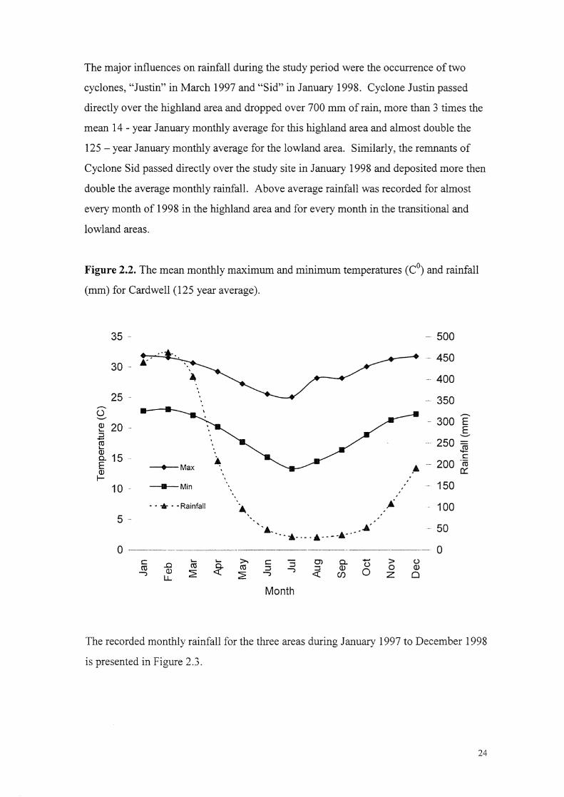
The major influences on rainfall during the study period were the occurrence of two
cyclones, "Justin" in March 1997 and "Sid" in January 1998. Cyclone Justin passed
directly over the highland area and dropped over 700 mm of rain, more than 3 times the
mean 14 - year January monthly average for this highland area and almost double the
125 - year January monthly average for the lowland area. Similarly, the remnants of
Cyclone Sid passed directly over the study site in January 1998 and deposited more then
double the average monthly rainfalL Above average rainfall was recorded for almost
every month of 1998 in the highland area and for every month in the transitional and
lowland areas.
Figure 2.2. The mean monthly maximum and minimum temperatures (Co) and rainfall
(mm) for Cardwell (125 year average).
35 ~
30 -
25 --
-- 500
450
.~~ 400
350..-..
300 EE............
-_.- 250 =JQc:
~ -- 200 &150
100
._. 50
o()(])
o>oZ
........()
oQ..Q)
en
, -6;.. .A.... .6. ......
.. .. ..- . - . A· .. - .....
..cQ)
ll...
.. Min
--+-Max
.......... Rainfall
0-
5 -
10 _.
Month
The recorded monthly rainfall for the three areas during January 1997 to December 1998
is presented in Figure 2.3.
24

Figure 2.3. Recorded monthly rainfall (mm) for 1997 - 1998, for the three areas of the
study site.
E6))5=:r.otEc~ 41)1
3l)
XX)
100
04---r----.-----,-~~-.:t~W::::!!::;:s.~~~___,~_r____r_~___r-~_=;::It::;::~-~~~____,
r- oo 00 00 00 00 00 00 00 00 00 00 00
~ 0\ C\~ ~ 0'\ 0'\ ~ C\ C\
~0'1 ~
u==
1:> l5.. >. § "3 be 6.. >- uC) coo It) ro coo = It) u 0 Q.)
Q ~ ~ :E <: ~ ~~ <:: C/) 0 z 0
Mrih
2.4. Ecological Parameters Chosen to Indicate Ecological Impacts of Feral Pigs
Within rainforests, the interactions of ecological parameters are too complex to
completely evaluate the impacts pigs may be having on the natural values of the WHA
as a whole. To quantify ecological impacts of feral pigs, specific ecological parameters
must be defined. Therefore, this study used selected ecological factors tenned
parameters as "impact indicators" to quantify aspects ofpig impacts on this rainforest
environment. The effect that pigs have on these parameters will indicate the impact
feral pigs may have on the general WHA rainforest and associated ecosystem.
A general discussion below provides an overview of the importance these parameters
have on the ecological processes within rainforests and the possible interaction these
parameters may have on pig ecology. Background information is provided to establish
why these parameters were selected for special study and the impacts that pigs may have
on these parameters.
Population parameters of feral pigs are dependent to a large degree on environmental
factors. While little infolIDation is available on pig population parameters in this region,
rainfall (soil moisture), food sources (earthwoffi1s, seedlings and plant roots) and surface
25

These selected parameters are thought to have particularly strong effects on seasonal
distribution patterns and reproductive success (Pavlov et al. 1992; McIlroy 1993;
Mitchell 1993) and will be discussed separately.
2.4.1 Rainfall
Water availability is extremely important to pig population dynamics (Giles 1980; Hone
1990; Bowman and McDonough 1991; Choquenot et at. 1996). The availability of
water for drinking and the amount ofrainfall detennining plant growth is the primary
limiting influence on population levels, particularly in the dry temperate and dry tropical
areas (Caley 1993b) although this influence is unquantified within the WHA. The
extent and temporal pattern of rainfall may also influence other ecological parameters
such as earthwonn populations and litter levels. The complex interrelationships of
rainfall, vegetative growth and nutritional availability is believed to be important to the
ecology of feral pigs within the WHA.
2.4.2. Food Sources
The amount and distribution of food resources is an important component of feral pig
ecology. Within the WHA the extensive array of plant, animal and invertebrate species
provide a broad array of potential food sources for the feral pig. For the purposes of this
study, the potential food sources that are most likely to be affected by pig diggings,
seedlings, earthwonns, and plant roots, have been chosen for special study.
2.4.2.1. Seedlings
No quantitative information on the importance of seeds and seedlings in the diet of feral
pig is available for the Wet Tropics region. The availability and distribution of the high
nutritional value seeds and seedlings may be an important influence on such aspects of
pig ecology as population distribution, reproductive parameters and survival rates.
The impact that feral pigs have on seed gennination and seedling survival is also
unquantified. Overseas studies suggest that feral pig diggings have a negative impact on
seedling germination and survival. Ralph and Maxwell (1984) found in Hawaii that pig
diggings significantly reduced the number of seedlings. Bratton (1974) found in the
USA, that pig diggings reduced under-storey cover by 85% to 92% and significantly
26

reduced the number of plant species present. Singer et al. (1984) found an 80%
reduction of seedling cover in diggings compared to undisturbed vegetation.
The importance of seeds and seedlings to feral pig ecology, while unknown in this
region, is thought to be significant. Also, the direct impact of feral pigs on seed
germination and seedling survival is relatively straightforward and measurable. Because
of these two factors, quantification of the impact of feral pigs on seedlings was chosen
as one of the impact indicators in this study.
2.4.2.2. Earthworms
Earthworms have been suggested as an important source of dietary protein for feral pigs
in this region (Pavlov et al. 1992; Mitchell 1993; McIlroy 1993; Choquenot et al. 1996).
Earthworms contain protein levels of over 60% (French et al. 1957). Feral pigs are
known to require a dietary protein level of at least 14% to sustain reproduction (Giles
1980; Pavlov 1991). The consumption of earthworms in sufficient quantities may
provide the protein requirements for pig populations to be sustained or increased by
maintaining reproductive rates. Lee (1985) stated that increased reproduction and growth
rates of semi-domestic pigs in New Guinea were due to a very high population of an
introduced earthwonn species that the local people collect and transfer to new pig foraging
areas. However, the relationship between earthworms as a dietary protein source and
pig population levels within the WHA has not been qualified.
Earthworms are also important food items for a wide range of rainforest fauna (Wroot
1985) and pigs may be an important competitor for this resource. Although earthworms
have been recorded as prey for small mammals such as bandicoots, small reptiles and
frogs, birds, centipedes, carabids etc, dietary importance of earthwonns to these animals
has not been adequately quantified. Earthworms also have high parasite loads of
nematodes and protozoa, and their role as intermediate hosts is probably significant
(Dyne 1991).
Earthwonns are an important component of the invertebrate macrofauna in tropical soils
(Lal 1987). Their action within the soil and litter leads to breakdown of plant material
and incorporation into the soil and recycling of subsoil nutrients. Earthwonns also aid
27

aeration of the soil and nutrient cycling by speeding up the decomposition cycle (Dyne
1991). Earthworms influence nitrogen recycling (Lee 1985), and surface casting causes
litter burial and hastens its decomposition into soil humus.
The WHA rainforests of the Wet Tropics harbour a diverse and ecologically interesting
earthworm fauna (Dyne 1994). Most species in the region (Cooktown to Mt. Spec)
belong to the genus Diporochaeta and to a lesser extent Diplotrema, Fletcherodrilus
and Begemius. The introduced glossoscolecid earthworm (Pontoscolex corethrurus) is
common in many disturbed highland sites. Populations of this exotic species may be
substantial, although less than reported in grassland habitats (Lee 1985). The impact of
this introduced species on the WHA endemic earthwonn fauna is unknown.
Transportation by bushwalkers and vehicles is probably responsible for their dispersal
although feral pigs may act as a dispersal agent through transport of soil containing eggs
and adults on their hooves and snouts (Spatz and Mueller-Dombois 1975). This
introduced species appears to be well established in rainforest areas disturbed by past
commercial forestry activities (Dyne 1991).
Disturbance has a marked negative impact on endemic earthworm populations,
especially the species that occur in the litter and upper soil layers. Pig diggings may
directly impact on native earthworm populations and indirectly influence nutrient
cycling through soil disturbance. In England, the native Lumbricus terrestris species
was found in higher numbers (150% to 600% more abundant) in undisturbed soil
compared to cultivated soils (Edwards and Lofty 1977). Reichle (1977) found that
when soil invertebrate communities were disturbed, soil detritus materials were rapidly
decomposed and subjected to mineral leaching. This was thought to be due to a bloom
of soil microflora with retention of nutrients in the microbial biomass.
Earthwonns can be divided into two morpho-ecological groups (Perel 1977) according
to their feeding habits i.e. (1) species that feed on or near the soil surface consuming
slightly decomposing plant residues (humus fanners) and (2) those species that feed on
decaying plant material within the soil structure (humus feeders). All are saprophagous,
some devour slightly decomposed material, even green leaf material, and others are
secondary humus feeders, feeding on material that has been decayed. The activity of
28

pigs may influence species composition of earthworm communities through direct
predation, introducing exotic earthworm species, or by modifying the habitat to favour
some species to the detriment of others. Modifying the species composition of
earthwonn communities may change the ecological processes involved in earthworm
feeding habits. This may in tum have a long term influence on the rainforest
environment.
Moisture loss by earthworms is an important factor in their survival, thus soil moisture
is an important ecological variable to earthworm populations. Lavalle (1983) found a
linear increase in earthworm biomass with increasing rainfall for various tropical
regions although the preferred range varied among species (Lal 1987). The preferred
soil moisture content in Nigerian rainforests was 23.30/0 (Madge 1969). Critchley et ale
(1979) related seasonal fluctuations in H africans populations to soil moisture and
temperature levels. The dependence of earthwonn population levels on suitable levels
of soil moisture may be an important factor influencing feral pig populations.
2.4.2.3. Plant Roots
There is a paucity of information on root distribution, dynamics and functions of roots
within the WHA. Roots are concentrated within the surface layers of the soiL Sam
(1995) estimated for rainforests that 78% to 94% of the total root biomass is
concentrated within the upper 30cm of the soiL Fine roots contribute less then 50% of
the root biomass but make up more then 90% of the root length and are an important
component of water and nutrient uptake.
Most of the root biomass is well within the reach of pigs. Kotanen (1995) suggested
that pigs will readily dig to 25cm in the soil profile. Although dietary studies of pigs
within the WHA are limited, visual examinations of stomach contents of sampled pigs
(Dorney pers. comm.) suggest that plant roots are a significant dietary component.
From personal observations, pigs actively seek the fine feeder roots, which have a high
nutrient composition that may attract feeding pigs. Two aspects of plant roots were
considered in this study; plant roots as a component of the diet of pigs and the impact
pigs have on plant roots by their digging action.
29

2.4.3. Litter
The litter layer is a component of the rainforest ecosystem as a reservoir of organic
material and nutrients; 65% of all soil nutrients are derived from the litter layer
(Schmidt 1991; Spain 1991). Pigs search in the litter for food such as small reptiles,
insects, amphibians and invertebrates. Litter also contains fallen fruits, fruiting bodies
of fungi and bodies of dead animals. Pigs may derive a significant portion of their
nutrition, particularly protein, from litter. Energy expended in searching the litter is low
compared to digging in the soil and the high nutritional rewards may make litter an
important component of pig ecology. The impact of disturbance of the litter by pig
diggings may change the decomposition rate of litter into soil humus which may
influence the amount and distribution of below ground plant biomass.
Litter fall has great variability and may be continuous or seasonal (Bray and Gorham
1964). Litter fall in the Wet Tropics is strongly seasonal (Brasell and Sinclair 1983)
with the maximum fall at the end of the dry season (November to February). Litter
usually builds up a dense layer over the soil by the start of the wet season, thus
providing some protection from the high intensity rainfall. The biomass of the litter
layer in the WHA varies from 2.5 to 7.4 t ha-1 in the lowland area to 3.5 to 11 t ha- l in
the highlands. Annual litter falls of 8 to 10 t ha-1 year have been recorded in the WHA
(Brasell et al. 1980). Foraging by pigs may influence the rate of litter breakdown by
mixing litter into the soiL Brasell and Sinclair (1983) described how the seasonal
variation of litter biomass depends on the balance between litter fall and decomposition
rates. The soil humus biomass, the product of decomposition of litter and dead root
material is found in the greatest concentration in the top 2.5 em of the soil profile and
accounts for 34% oftatal biomass (Laurance 1996), 50% of all soil animal biomass is
found in the top 10 cm (Fittkau and Klinge 1973). Breakdown rates in the Wet Tropics
rainforests (k ratio of mass of litter fall to the standing crop of litter) are comparable to
values from other tropical rainforests (Olsen 1963). Values range from a three year
mean of2.2 from a lowland site to 1.2 to 1.5 at four sites in the highlands (Brasell and
Sinclair 1983). Studies of leaf breakdown have shown that a considerable seasonal and
annual variation occurs in the nature and rates of breakdown depending on
environmental and species differences (Spain and Le Feuvre 1987).
30

Chapter 3
Spatial and Temporal Patterns of Feral Pig Diggings
3.1. Introduction
Most perceptions of the environmental impacts of pigs focus on their disturbance of
the soil or soil surface materiaL This activity has been variously described as digging,
rooting, ploughing or tilling. Simple measurements of soil disturbance (referred to
hereafter as diggings) are inadequate in quantifying the ecological impact caused by pig
diggings. However, a basic knowledge of the intensity and scope of diggings may
provide an insight into possible ecological impacts being caused, or facilitate the
implementation of management policies to reduce the perceived impacts.
Diggings have been used as an index of the ecological impact of pigs in overseas
studies (Rudge 1976; Howe et aL 1981; Stone and Taylor 1984; Loope and Scrowcroft
1985), and in Australia (Hone and Pederson 1980; Hone 1995; Mitchell and Mayer
1997; Vemes et al. 2001). Diggings have been implicated in causing erosion,
reducing water quality, changing litter composition and distribution, affecting nutrient
and water cycles, affecting soil invertebrate populations and soil seed banks, and
changing species succession patterns which influence long term ecological processes
(McIlroy 1993).
Belden and Pelton (1975) suggested a "rooting area index" had potential for monitoring
the abundance of feral pig populations. Katahira et al. (1993) and Ralph and Maxwell
(1984) found a positive relationship between the area of diggings and pig population
levels in Hawaii. However Hone (1995) and Cooray and Mueller-Dombois (1981)
found no significant statistical relationship between digging and pig abundance. The
nature of the relationship between population levels of feral pigs and the abundance of
their diggings is complex and still unclear.
Diggings have been used to quantify where pig impacts occur (Bratton 1974; Bratton
et a1. 1982; Hone 1988b; Hone 1995) and when they occur (Howe and Bratton 1976;
Alexiou 1983; Hone 1995). Hone (1995) suggested that the distribution of pig
diggings vary in both space and time and that the emphasis on identifying pig impacts
31

is often on the level or intensity of impact, but does not take into account spatial or
temporal variations of impacts or the causes of such variation. He described the
spatial variation of impacts as a frequency distribution (number of sites with a
particular level of impact) as a negative exponential frequency distribution; many sites
with few diggings and few sites with many diggings. Mitchell and Mayer (1997)
described spatial digging patterns at a broad scale within the Wet Tropics, with
lowland areas having a higher digging index than highland areas. They also found
variations in digging activity between microhabitats with higher levels of diggings
occurring within 10m of logging tracks and drainage lines. Hone (1995) described
temporal variation of impacts as dependant on an index in pig abundance (such as
diggings) in relation to seasonal conditions. Temporal variation of feral pig diggings
have been suggested in other studies within the Wet Tropics (Pavlov et al. 1992;
McIlroy 1993; Laurance and Harrington 1997; Vernes et a/2001).
To achieve effective feral pig management it is essential to first quantify the nature
and scope of their impacts; where, when and how much is occurring. One objective
of this particular study is to quantify the spatial and temporal patterns of a specific
impact i e. soil disturbance caused by feral pig digging activity (Objective 1, Chapter
1.2). Spatial patterns will clarify preferences of feral pigs to dig in specific
microhabitats, and temporal patterns will examine the effect of seasons on digging
activity. The second objective (Objective 2, Chapter 1.2) is to monitor soil moisture
and earthwonn populations as previous studies have suggested that digging activity
appeared to be correlated with soil moisture (Hone 1988a; Hone 1995), soil friability
and possibly the presence of earthworms (Pavlov et at. 1992; McIlroy 1993).
3.2. Methods
3.2.1. Digging Transects
The three distinct areas described in Chapter 2 were used to define the main
biogeographical features or macrohabitats identified in the study site. Each of these
areas were further categorised into different strata as defined in Chapter 2,
representing the main microhabitat types occurring in each area. Three replicated sites
were then randomly selected within each stratum with sites approximately 2 to 10 km
apart. Within each of these selected sites, five 50 ill line transects were then
established with transects positioned 50 to 100 m apart.
32

Each transect consisted of two wooden pegs positioned 50 m apart so a measuring tape
could be tightly positioned on the ground between the pegs. Marked trees within the
transects were used to enable accurate re-positioning of the tape for each sampling
event. The 50m transect was categorised as a continuous series of 500 increments, each
of 10 cm. Increments, as identified on the measuring tape, that passed directly over
feral pig diggings or were unavailable to pigs due to fallen trees or covered by water
(more then 10cm deep) were recorded. In total, 195 transects, covering 9.75 lan, were
established and monitored. The number of selected strata and established transects for
each area is shown in Table 3.1.
Increments that passed over pig diggings or were unavailable to pigs were mapped on
graph paper. These transect maps allowed the identification of increments that were
dug in the previous sampling event so that diggings observed at subsequent sampling
event could be identified as old (previously recorded) or as new (occurring since the last
sampling event). The proportion of available increments on each transect that had
been disturbed by new pig diggings between successive samplings was termed the
"digging index" and provided the basic data for analysis. The appraisal of new diggings
was also backed up by a subjective appraisal of the age of diggings based on the amOlli1t
of litter in the diggings and dryness of the soil. Rain, leaf litter and the scratching
activity of scrub turkeys (Alectura lathami) and scrub fowls (Megapodius reinwardt)
sometimes masked diggings caused by feral pigs.
Transects were established in April 1997, and all initial diggings on each transect were
recorded to establish the amount of "previous" diggings that were present. Transects
were then re-sampled (tenned sampling events) 10 times i.e. (July 97, September 97,
November 97, December 97, February 98, May 98, June 98, August 98, October 98,
and December 98). The timing of sampling events was dictated by weather conditions,
flooding and road closures so to some degree sampling was conducted on an irregular
basis.
33

Table 3.1. The number and name of all strata, and the number of sites and digging
transects that were established within each of the three areas.
Area
Highland Transitional Lowland
Strata (n) 5 2 4
Strata Creek Creek Creek
Track Track Track
Swamp Swamp
Ridge Forest
Road
Sites (n)...,
6* 3.)
Transects (n) 5 5 5
Total (n) 75 60 60
Total length (km) 3.75 3.0 3.0
* Note - As only two strata were selectedfor study in this transitional area, 6 sites were established
instead of3 in the other areas, to increase the database size.
3.2.2. Ecological Sampling
Two ecological parameters were sampled in conjunction with diggings; earthwonn
biomass and soil moisture levels. For each transect, a sample site 1 m adjacent to the
transect was cleared of leaf litter and llitre of soil collected from a 25 em3 hole and
stored in a numbered plastic bag. Sample sites were selected at the 10 ill mark for
sample event 1 ,20 m at sample event 2 etc. Each soil sample was hand sorted and all
earthworms were removed, placed in numbered 50 ml bottles and covered with 10%
fonnalin. After the earthworms were removed, one soil sample from each site (three
replicates of each stratum) was selected for soil moisture measurement (transect 1 in
sample event 1; transect 2 in sample event 2 etc). The sample was weighed, dried at
70°C for 4 days and reweighed to derive moisture content (%).
EarthwOlTI1S were stored until the next sampling event (1 to 2 months) in formalin to
standardise their body weight. As earthworm body weight is directly related to the soil
moisture levels, storage cause the earthwonns to reach saturation with formalin so wet
34

weight would be directly correlated with body mass. This method resolved the
problem ofbody weight bias caused by varying soil moisture levels. Earthworm
biomass was measured as wet weight (g), after being pat-dried with tissue paper,
weighed and replaced into the same bottle for future identification. Satchell (1971)
reported that after 1 month in fonnalin earthworms lost 12.9% of their body weight.
Monthly rainfall recordings for each area were used to define seasons. The digging
index was defined as diggings that occurred from the previous sampling event, so
each sampling event was classified into a season category based on the rainfall
preceding each sampling event. A special case arose for the first sampling event,
April 1997, when Cyclone Justin completely destroyed or masked all diggings so the
original digging index recordings started in January 1997 could not be used. The
diggings recorded in the April 1997 sampling event were deemed to have occurred
since Cyclone Justin (March) and were categorised as "wet season" due to the severe
rainfall event of this Cyclone (Figure 2.3).
3.2.3. Analysis
The calculated proportion of the available increments in each transect between each
sampling event that was disturbed by new feral pig diggings was termed the "Recent
Digging Index" (RDI). Interpretation of the RDI was complicated by the differences
in the number of days between the sampling events as the amount of recent (fresh)
diggings would presumably be related to the amount of time available to cause these
diggings. To resolve this problem, a standardised digging index was calculated as the
amount of recent diggings that occurred in a time period of one day. This diggings
index was termed the "Daily Digging Index" (DDI) and was used in all statistical
analysis to detennine statistically significant spatial and temporal differences between
strata.
The DDI was recalculated from the RDI using the following equation
DDI = (x / (500 - n)) / d
x = number of increments positive to pig diggings, n = number of increments
unavailable and d = number of days since the last sampling event.
35

Analysis assessed spatial and temporal digging patterns for each stratum within each
area. One way ANOVA was used to test for significant spatial variation by comparing
DDI data populations between the strata in each area. A Tukey Test was applied to
demonstrate significant strata differences within each area between the strata means for
all sampling events combined and between the strata means for each sampling event.
Repeated measures ANOVA was used to test for significant temporal variation
differences between strata over all of the sampling events. The interaction between
strata and the time of sampling was also tested. Plots Were constructed to illustrate
trends of variations in diggings between strata over time. Two-way ANOVA and Least
Squared Regression analysis was used to compare strata digging patterns with the two
measured ecological variables (earthwolTIl biomass and soil moisture) for all sampling
events.
The proportion of each transect that recorded any pig diggings, across all sampling
events combined, was also calculated and termed the "Total Diggings Index". One
Way ANOVA and Tukey test examined differences in the total digging index between
the strata within each area. The frequency (%) of transects in each site that recorded
any diggings at each sampling event was also used to calculate a "Frequency of
Diggings Index". Digging frequency was modelled as linear regression to measure
the effect of strata and season on digging frequency.
The mean DDI for each stratum for sampling events categorised into the three seasons,
dry 1997, wet 1998 and dry 1998 was calculated. Two - way ANOVA demonstrated
the variations in seasonal diggings among strata. The relationship of rainfall patterns to
the digging index was analysed by regression of the mean DDI on the lagged rainfall
that was recorded one to eight months previously.
36

3.3. Results
3.3.1. Digging Index
The overall mean RDI for each area was 0.08 (8%) in the highlands, 0.045 (4.5%) in
the transitional and 0.05 (50/0) in the lowland. The overall mean RDI for the three
areas was 0.0587; approximately 6% of each transect was disturbed by feral pigs
between each sampling event.
The calculated mean Daily Digging Indices (DDI) for each stratum, in each sampling
event, in the three areas are presented in Table 3.2. The mean DDI for all strata
combined was 0.115 ± 0.036% for the highland area, O. 077 ± 0.0337% for the
transitional area and 0.076 ± 0.038% for the lowland area. The overall mean DDI for
all strata in all areas was 0.09%.
Differences in the amount of digging activity between the different strata (spatial
differences) were identified. Significant overall mean DDI differences between the
strata (means for all sampling times) were detected in the highlands (F4,lO = 9.95, P <
0.01) and transitional areas (F1,lO = 8.03, P < O.05)but not in the Lowland area (Figure
3.1). In the highland area, swamps had significantly more pig diggings than all other
strata, and creeks had a significant higher digging index than roads. No differences
were found between track, road and ridge strata. The order of highest mean pig
digging activity ranged from swamp, creek, road, track, to the least diggings in ridges.
In the transitional area, creeks had significantly more pig digging activity than tracks.
No significant mean strata differences were detected in the lowland area. Strata
ranked from the highest to lowest digging activity were swamp, creek, track and
forest.
37

Table 3.2. The mean (%) daily digging index (DDI) for each stratum for all
sampling events within each of the three areas.
Highlighted values indicate where significant differences between strata values were
detected Values followed by the same superscript letter are not significantly different.
Area Strata Sampling events and days (n) between each event
Jul-97 Sep-97 Nov-97 Dec-97 Feb-98 May-98 Jun-98 Aug-98 Oct-98 Dec-98
(100) (56) (48) (37) (61) (77) (57) (57) (47) (63)
Highland Swamp 0.56 a 0.44 a 0.24 0.12 ab 0.14 0.32 0.44 a 0.35 0.17 0.17
Track 0.05 be 0.01 b 0.0 0.0 b 0.07 0.09 0.08 b 0.0 0.03 0.11
Ridge 0.002 c 0.02 b 0.0 0.0 b 0.01 0.0 0.0 b 0.0 0.0 0.0
Road 0.61 a 0.0 b 0.0 0.0 b 0.0 0.22 0.04 b 0.0 0.01 0.0
Creek 0.36 ab 0.0 b 0.2 0.27 a 0.02 0.22 0.25 ab 0.08 0.01 0.07
Transitional Creek 0.07 0.52 a 0.05 0.01 0.04 a 0.1 0.09 0.27 a 0.22 0.07
Track 0.01 0.0 b 0.003 0.005 0.01 b 0.01 0.03 0.01 b 0.02 0.01
Lowland Creek 0.33 0.02 0.0 0.07 0.14 0.0 0.26 ab 0.0 0.07 0.06
Swamp 0.22 0.25 0.1 0.04 0.04 0.09 0.14 b 0.2 0.13 0.05
Forest 0.03 0.001 0.0 0.01 0.0 0.03 0.01 c 0.0 0.0 0.01
Track 0.11 0.0 0.01 0.04 0.1 0.05 0.39 a 0.03 0.01 0.03
Significant differences in diggings were also found between the strata at some
individual sampling events (bold in Table 3.2). Significant differences (F4,IO = 6.34, P
< 0.01) in the highland area for July 1997 were found between swamps and roads,
which had significantly more diggings then tracks and ridges, and creeks had
significantly more diggings than ridges. For September 1997, significant differences
(F4~IO = 7.00, p < 0.05) between strata were detected, swamps having significantly
more diggings then all other strata. In June 1998 there were significant variation
among strata (F4,IO= 3.6, p< 0.05) swamps and creeks had significantly more diggings
than track, ridge and road strata.
38

Figure 3.1 Mean daily digging index (and s.e.) of each stratum over all sampling
events for the (a) Highland Area, (b) Transitional Area and (c) Lowland Area.
(a) Highland Area
3.5 ..
o
Creek
(b) Transitional Area
Swamp Track Ridge Road
3.5 -
3 -
2.5 -
2 -
1.5 .'
1 -
0.5
0---------
(c) Lowland Area
Creek Track
3.5 ~
3
2.5 ..
2-
1.5 -.
1
0.5
o
Creek Swamp Track Forest
39

For the transitional area, significant differences between strata were found in the
September 1997 (F1,10 = 8.84, P < 0.05) February 1998 (F1,IO = 6.24, P < 0.05) and
August, 1998 (F1,10 = 5.46, p < 0.05) sampling events. More diggings were found in
creeks than in tracks. For the lowland area in the June 1998 sampling event,
significant differences (F3.8 = 5.39, P < 0.05) between strata were detected with
creeks having significantly more diggings than the forest, and tracks having
significantly more diggings than swamp and forest.
Differences in the amount of digging activity between the sampling events (all strata
combined) were identified in the highland area (F3,11 = 5.22, p < 0.01), the transitional
area (F2,2 = 4.43, p < 0.05) and in the lowland area (F3,9 = 4.43, P < 0.05). A
significant strata by time interaction effect was detected only in the transitional area
(F2,20 = 4.55, P < 0.05).
Temporal differences in the amount of digging activity for each stratum between each
sampling event were also detected. In the highlands, significant differences between
sampling events were detected in the road stratum (F9,20 = 7.1, P < 0.001) where the
July 1997 sampling event had significantly more diggings than all other sampling
events, and for the creek stratum (p = 0.03, ANOVA with ranks SNK test) more
diggings were detected in the July 1997 than in the September 1997 sampling event.
For the transitional area, the creek stratum had significant differences (F9.20 = 3.41,
p< 0.01) between the September 1997 and all other sampling events except August
and October 1998 sampling events. For the lowland area the creek stratum had
significant differences in DDI between sampling events (F9,20 = 3.66, P < 0.01). More
diggings occurred in the July 1997 and February, June and August 1998 than all the
other sampling events. Temporal trends in digging activity for the study period are
presented in Figure 3.2.
40

Figure 3.2. Temporal variations in the mean daily digging index for each stratum
within the three areas
(a) Highland Area
0.007 -
0.006 -
~ 0.005 -"0c:~ 0.004 .-c'0,0>is 0.003 ->.
~ 0.002 -
0.001 -
0.000 -
0.007 -
0.006 -
x 0.005 Q)
""CC
~ 0.004 ..c
'(5)Ol5 0.003 -~'roCl 0.002 -
0.001
o -
0.007 -
0.006 _.
0.005 -
(b) Transitional Area
(c) Lowland Area
_Swamp
~Track
--.-Ridge
--e--Road
,--'-Creek
xQ)
"'CC
~ 0.004 -c'6>Cl
o 0.003 :?:-'roo
0.002 ..
0.001 .-
oI'- I'- I'- I'- l' l' ,...... J"-. l' co co co co co co co co ex:> co co coq> 0) q> O? q> q> or 0) 0'> q> 0'> q> q> 0) O? q> 0) 0> q> 0> 0)
~>. c: :i Ol c.. t5 > U c .D Co ~
>. c :i en a. t5 > 0ro :J """")
~Q)
0 0 Q) ro Q)
~ro :::J -,
~Q)
00 Q)
:2 -, en z Cl -, LL 2 -, en z 0
Month
41

3.3.2. Associations of diggings with rainfall patterns.
Digging patterns showed a negative association with rainfall, less digging occurred
during the wet season and conversely most diggings occurred during the dry season
(Figure 3.3).
Figure 3.3. Relationship of (a) mean digging index (for all strata) within the three
areas and (b) recorded rainfall (mm).
(a) Mean digging index
0.004 '
0.003-
0.003 -x(1)
~ 0.002 -Olc·en 0.002 Ol
Ci0.001 -
0.001 ".
0.000 --
_Highland
--e-- Transitional
--.- Lowland
1000 -
comUQ)(:)
coQ)
>oZ
r- co coCJ) q> Q)
u c .nQ) ctl Q)
0 J lJ..
Month
r- r- t'- I"m 0) q> men n 13 >~ tJ5 0 ~
300
200
100 ..
o ~._._---_ ..__.__._---_.~-=::~ __~~~~::::tI~~~r- r- r- r- r- r- r-~ ~ q> q> t '% q>
~ ~ ~ ~ ~ ~ ~
900 .- (b) Rainfall
800 -
700 .
E 600-.s500 ,.
JQ·ffi 4000::
The mean strata DDI within the sampling events that were categorised within the four
seasonal sampling events of wet and dry 1997, wet and dry 1998, were calculated for
each season category (Figure 3.4). A two way ANOYA indicated no significant
differences in strata mean diggings between the seasons in any of the three areas, and
no significant season/strata interactions, but confirmed significant differences
occurred between strata means within each season.
42

Figure 3.4. The mean stratum digging index for the combined sampling events
categorised into the four seasons.
(a) Highland Area
--'-swamp
-B-track
--*-ridge
--*-road
4.5
4xQ) 3.5-0.5 3C)c 2.5"a'C) 2
=0~ 1.5·co 1o
0.5
Ot--_G=======:::;::::===~;;;;::~~---6----"'----=:::::~-----,wet dry wet dry
(b) Transitional Area
--'-creek
-B-track
4.5
4x~ 3.5.5 3C)
c: 2.5'0,C) 2
i 1.~ 11
0.5
o -!-I ~G:::====::::::::;::==~,Q-_=========:I~~====;:=:====~L-__---.wet dry wet dry
drywet
--'-creek
-B-swamp
--*-woodland
--*-track
dry
0.5 "1I
o +~----JAk:=======;:=====::J·Ik:=:==:::::::::::::;:::::::::::::::::::::::::::j·IIr:======;:::==~~A~--____,
wet
(c) Lowland Area
4.5 l4 ....
8 3.5 I~
.s 3b.()
.S 2.5b!)
.~ 2""0..Q 1.5.t; 1o
Seasons
The association of individual stratum diggings with lagged rainfall is presented in
Figure 3.5. Significant (p < 0.05) R2 values for the regression of rainfall with the
strata mean in each area were found between three and four months lagged rainfall in
the highlands, and five months in the transitional and lowland areas.
43

Figure 3.5. The relationship of digging index (for each stratum within each area) to
monthly rainfall lagged 1 to 8 months previously. Plot of the calculated R2 values for
the relationship of the DDI in each stratum with each lagged (by month) rainfall
event. Note * = significant R2 values
(a) Highland Area
0.9
0.8
0.7
0.6U'J<D:Jco>a::::
0.3
0.2
0.1
0
--+-Swamp
_Track
--.-Ridge
~~ - --*- Road
~Creek
.......HighAv
--+-Qeek
---II- Track
....... TranAv
Lagged Rainfall- months
(b) Transitional Area
0.8
0.7
0.6
t/) 0.5(])
~ 0.4>a:: 0.3
0.2
0.1
O+--------,-------.-----........,.....-----,..--------r-----..----~3 4
Lagged Rainfall- ITOnths
(c) Lowland Area
0.8
0.7
0.6
C/) 0.5CD:::J
0.4ro>0:: 0.3
0.1 I
o I0
--+-Creek_Swamp
--.-Woodland
--*-Track
.......LowAv
•
Lagged Rainfall- months
44

3.3.3. Frequency of diggings.
The frequency of transects within each stratum that recorded any digging on the
transect length at each sampling event, were converted to a frequency distribution and
are presented in Figure 3.6. In the highland area, a significant difference in frequency
of diggings on transects between strata was detected (F4,lO = 15.19, P < 0.01). All
other stratum had a significantly higher mean digging frequency than the ridge
stratum. In the transitional area significant strata differences were detected (F4,IO =
13.24, P 0.01), with higher frequency of diggings occurring in creeks than in the
roads. No significant differences between strata were detected in the lowlands (p >
0.05). The highland area had a mean transect digging frequency for all strata of27%,
transitional 15% and lowland 280/0. An overall mean transect digging frequency for
all strata within the three areas was calculated, on average 23% of transects were
affected by some diggings at each sampling event.
Figure 3.6. Frequency of occurrence (and s.e.) of diggings occurring on transects
within each strata for the three areas for all sampling events.
0.6 -
0.5 -
0.1 -
en0)
's, 0.4 -0)
~
~ 0.3-ucQ)
:J0" 02-~ .u..
Swamp Track Ridge Road
Highland
Creek Creek Track
Transitional
Strata
Creek Swamp Forest Track
Lowland
Temporal differences in frequency of diggings between strata were also detected. For
the highlands significant differences in diggings between strata were detected in July,
September and December 1997 and June, August and October 1998, all regarded as
dry season samples. For the transitional area, significant differences in digging
45

frequency between strata occurred in September 1997 and February and August 1998a
For the lowland area, only one sampling event, June 1998, recorded significant
differences in digging frequency between strata. In almost all cases significant
differences in transect digging frequency between strata were detected in the dry
season monthsa Significant strata differences are presented in Table 3.3a
Table 3.3. Frequency of transects within each stratum that recorded any digging for
each sampling event, for each area.
Highlighted values indicate sampling events where significant differences in
frequency ofdiggings were detected between strata. Values followed by the same
letter are not significantly different.
Area Strata Sampling Events Mean
Jul97 Sep97 Nov97 Dec97 Feb98 May98 Jun98 Aug98 Oct98 Dec98
Highland Swamp 0.8 3 Oa73a 0.4 0.273 0.33 0.6 0.83 0.533 0.333 0.4 0.523
Track 0.4 b 0.07b 0 OC 0.27 0.27 Oa47cd Ob O,,13b 0.4 0.23
Ridge O.07c 0.07b 0 OC 0.07 0 Ob Ob Ob 0 O.02b
Road 0.933 Ob 0 OC 0 0.47 0.2bc Ob O.07b 0 0.173
Creek 0.873 Ob 0.47 O.6b 0.07 0.73 Oa733d 0.43 0.13b 0.17 0.423
0.2 Oa07b 0
Transitional Creek
Track
0.33 0.533 0.07 0.07 0.273 0.33 0
0.07 0~07 Oa13b 0
0.473 0.13 0.13 0.233
o
Lowland Creek 0.8 0.27 0 0.2 0.4 0 0.13 0.2 0.29
Swamp 0.73 0.6 0.2 0.2 0.4 0.2
Forest 0.27 0.07 0 0.07 0 0.2
Track 0.73 0 0.13 0.2 0.4 0.2
0.733 0.6 0.4 0.27 0.43
Oa13b 0 0 0.27 0.1
Oa733 0.27 0.2 0.27 0.31
Temporal trends in frequency of diggings for the three areas are presented in Figure
3.7. Seasonal trends in digging frequencies are similar to the trends in DDI, showing
cyclic patterns of digging frequency associated with seasonal influences. Higher
digging frequencies occurred in the dry seasons, lower frequency of diggings occurred
in the wet season.
46

Figure 3.7. Seasonal trends in digging frequency for the means (s.e) of all strata
within each area.
0.7 ~
0.6 -
0.5 -
>.()c:~ 0.4 -0""Q)
Li:en.5, 0.3 -0>
C5
0.2 -
0.1 -
-+-Highland
-.-Transitional
---.- Lowland
._=---A_~_~~~~~ .._.
0- ~~·~w·~,·___·~~~~~~_~·~_
f'.. f'.. f'.. f'.. f'.. t"- t"- t"- f'. ex;) ro co co ex;) co co co co co co coq> en 0) q> en 0) 0( (j') en q 0) q> q> (j') 0)
~CJ) 0)
~(J) 0'>
~~ C :i 0, a. u :> u c:: ..0 ro ~
~ C ::J0, 6. t5 :> u
C'O ::J -,~
Q)0 0 Q) C'O Q)
:2C'O ::J -, <t Q)
0 0 Q)
:2 -, en z 0 -, u. :a --, (/) z 0
Month
3.3.4 Total Diggings
The mean proportion of transect increments (in each stratum) that were disturbed by
pig diggings at any time during the study period is termed "total diggings" (Figure
3.8). In the highlands, significant differences (F4.l4 = 12.3, P < 0.01) between the total
diggings in each stratum were detected, swamps having more total diggings than all
other strata except roads, while roads had more total diggings than the ridge stratum.
For the transitional area, significant strata differences (F4,14 = 10.4, p< 0.05) were
detected with higher total diggings occurring in creeks than in tracks. There was no
significant difference in total diggings between strata (F4,14 = 2.2, P = 0.19) in the
lowlands. For all three areas, there was no significant site interaction effect (p > 0.05)
47

Figure 3.8. Total diggings for each stratum within each area. The mean percentage
(and s.e.) of transect increments that were disturbed by pig diggings at any time over
the total sampling period.
100 ~
9O~
80 ~
70 ~ Highland TransitionalfI)
0> _......c'5> 60 -0>
:.0co 50 ~
:90
40 -~0
30 ~
20 ~
10 ~
Lowland
,...::=, n~ __fJ) fI) C1> "0 .x. ..::.::: fI) fI) fJ) fI) en0. .x. 0> co C1> (1) .x. ..::x::. 0.. "0 ..::x::.E c.> "0 0 Q) C1> U Q) E c u
CO a: 0:: U 0 co Q) (\$ men~ ~ u ~ =a ~;:
en (J) 0
~Strata for each Area
3.3.5 Ecological interactions with diggings
Strata means of earthworm biomass and soil moisture are presented in Table 3.4.
The mean earthworm biomass for all strata for all sampling events was 2.1 g m3 in the
highlands, 1.5 g m3 in the transitional and 1.1 g m3 in the lowland areas. Earthworm
biomass appeared to fluctuate with seasonal rainfall patterns, the greatest biomass
occurring during the late wet, early dry season (Figure 3.9). For all of the three areas,
a trend of increasing earthworm biomass during 1998 corresponded with the higher
than normal rainfall for this period. High earthworm biomass persisted as the higher
than normal soil moisture levels were maintained throughout the 1998 dry season.
Soil moisture trends are shown in Figure 3.10 illustrating the higher than normal
rainfall throughout the 1998 period.
Regression analysis was used to detect if any significant associations existed between
diggings, earthwonn biomass and soil moisture levels. In the highlands, a significant
positive linear association between soil moisture and earthwonn biomass was detected
for roads (R2= 0.31; F1)8 = 12.53, p < 0.01), tracks (R2 = 0.33; Fl~28 = 13.96, P <
48

0.01), and ridges (R2 = 0.22; F1,28 = 6.9, p<0.05). A significant positive association of
diggings with soil moisture was also found in the creek stratum (R2 = 0.26; F1,28 =
4.87, P < 0.05). A significant positive association was found in the transitional area
between soil moisture and worm biomass in the creek (R2 = 0.14; F1,S7 = 9.18, P <
0.01) and track stratum (R2 = 0.44; F 1,S8 = 45.0, p < 0.01). For the lowland area a
significant positive association between pig diggings and earthworm biomass were
found for swamps (R2 = 0.22; F1,28 = 3.85, P < 0.05) and forest strata (R2= 0.26; F1,28
= 4.77, P < 0.05).
Table 3.4. Mean earthwonn biomass (glro3) and soil moisture levels (%) for each
stratum within the three areas.
Area Strata Earthwonn Soil Moisture
Biomass (glm3) (%)
Highland Swamp 1.7 33.4
Track 2.8 17.3
Ridge 3.2 21.5
Road 2.1 13.6
Creek 0.5 14.2
Transitional Creek 1.9 20.5
Track 1.1 13.6
Lowland Creek 2.7 28.8
Swamp 0.4 42.8
Forest 1.0 18.2
Track 0.3 8.5
49

Figure 3. 9. Temporal trends in earthwonn biomass for each stratum, within each
area.
(a) Highland Area
0.9
E 0.8.9:E 0.7C)
~ 0.6
E 0.5a~ 0.4CDg> 0.3Q;~ 0.2
0.1
o
--+-swamp____ track
-..-ridge--*-road-e-creek......average
(b) Transitional Area
1
0.9
10.8
:E: 0.70>
~ 0.6
E 0.5o~ 0.4CDg 0.3
~ 0.2<{
0.1
o
-e-creek____ track
......average
(c) Lowland Area
coen
It)CDo
coc»I
>oZ
ex) co0) 0">
1 ICl. ....Q) (,)
C/) 0
ex)0')
I
0>::J«
co0'>,S-,
CX) 0::> 000'> 0) 0'>
I I I.0 '- l-ID co ~
u. ~ <C
Month
0:>0)
Ic:co-,
tO'>,
C,,)Q)
o
tO)
I
>oZ
t- tO) 0)
I ICi.. ......,Q) (.)
C/) 0
-e-creek--+-swamp____ track
--Is- forest......average
0.1
o-l.*~~~.!;::::& ....~~=-=~~...--......-::;==*:~~~-,,....-----,--~~
0.9
E 0.8C)
~ 0.7C)
'(j) 0.6?;E 0.5a3: 0.4
CD
g> 0.3as~ 0.2
50

Figure 3. 10. Temporal trends in soil moisture levels (%) for each stratum, within the
three areas.
(a) Highland Area
60
50
10
o
--+-Swamp
---Track-.tr-Ridge
--*-Road--.-Creek
.....Average• -AfT
(b) Transitional Area
60
50--+-Creek____ Track
~ 40 -.-Averagee-O)
::;(;) 30·0~
·0 20(f)
10
0
(c) Lowland Area
50
--+-Creek___ Swamp
-.tr- Forest
~ --*-Track~ \ .....Average
~
,....... ,....... ,....... l"'- I"'- t-- eo co co co co co co 0:;) ro co CCl coc.n Q) c.n Q) 0) 0) c.n 0:- m c.n m 0) Q) 0) OJ m 0) 0">I I I I I I I I I I I I I I I I I I
"S 0) c- o > u C ..0 L.. L.. >, C S 0) c.. t5 > C,,):J Q) 0 (l) co CD co Cl. co ~ :::J Q) 0 Q)J « CfJ 0 Z 0 J u.. ~ « 2 J
J « (j) 0 Z 0
Month
51

3.4. Discussion
Diggings or soil disturbance by feral pigs is their most obvious visual impact on the
environment~ Quantifying diggings in terms of patterns (or trends) has allowed an
insight into the preference of pigs to dig in specific microhabitats and the seasonality of
this digging preference~ Spatial and temporal patterns of feral pig diggings were found
in this study during the two-year study period~ In general, pigs preferred to dig in
specific moist microhabitats (swamps and creeks) and most of these diggings occurred
at a specific time (season) of the year; the early dry season~ Rainfall (soil moisture)
appeared to be closely related to these digging pattems~
Differences in digging indices between the three areas were apparent, the highland
area recording more diggings than the transitional or lowland areas. This difference
may indicate either pig population densities are higher or that digging is a more
prominent foraging activity in this highland area~ The lack of standardisation of strata
types between the areas and the fact that the selected strata types represent only a small
proportion of the total area precludes a direct comparison of total pig activity between
the areas based on digging indices alone~ Mitchell and Mayer (1997) reported a
contrasting result in their dry season study where they found significantly less diggings
in the highlands compared to the lowlands (2.41 % compared to 8~91 %), although their
different survey designs from this study may confound this comparison.
Differences in the level of diggings between the strata were found in all three areas~
Pigs preferred to dig in swamps and creeks, possibly due to optimal soil friability and
soil moisture levels~ Most diggings occurred in strata that represent only a small
portion of the total area. Swamps and creeks for example, occupy only small areas, but
have the highest digging indices~ In comparison, the strata that represent a large portion
of the total area, ridge in the highlands and woodlands in the lowlands, had significantly
lower digging indices. The trend was for most diggings to occur within the localised
microhabitats and not within the large scale habitat (the general forest floor). Thus
potential ecological impacts of pig diggings may be concentrated within only small
areas of the WHA and may not be an important impact to the WHA general rainforest
habitat.
52

The digging indices were significantly associated with soil moisture levels and tended
to be strongly seasonaL The increased level of diggings in the dry season may be
associated with pigs being attracted to moist soil as it is easier to dig (less energy
expenditure), underground plant bulbs and earthworms may be present and to wallow
in the cool soiL Mitchell and Mayer (1997) also found most pig diggings occurred
within 10m of drainage lines or wet areas within the WHA, Vemes et al (2001) found
significantly more diggings in swamps than in ridge microhabitats. The preference for
digging in wet areas was also found in the USA (Bratton et aL 1982) and France
(Dardaillon 1987).
The observed spatial digging patterns consists of most diggings occurring in favoured
microhabitats of small overall area and less digging occurring in less favoured
microhabitats of large overall area. Hone (1988b) described this digging pattern as a
negative exponential frequency distribution. This spatial pattern was also found in the
WHA by Mitchell and Mayer (1997) who found significant differences in spatial
digging activity between microhabitats, ranging from 16% in drainage lines, 8% in
roads, to 2.4% in the general forest floor. Laurance and Harrington (1997) found spatial
digging pattern between WHA forest types with more diggings occurring in wet
sclerophyll forests compared to rainforests and woodlands.
The digging indices were extremely variable in terms of space, between strata, and time,
between the sampling events due to changes in digging preferences or changes in
population density. The amount of diggings recorded on a transect ranged from a
maximum of 61 % on a road stratum transect in the dry season in the higWand area to no
diggings recorded in at least one sampling event (both seasons) in all strata (except the
highland swamp stratum). No comparable Daily Digging Index results are available
from other pig studies, however, comparison of reported cumulative digging indices is
possible. The overall mean recent digging index for all strata in the three areas was
calculated at 60/0. This is comparable to Mitchell and Mayer (1997) WHA late dry
season study where they found a similar cumulative pig digging index of 4.14%.
Vemes et al (2001) found a 2.30/0 of new diggings over a three week period.
Comparable Hawaiian rainforests studies have reported higher digging indices of 14
38% (Cooray and Mueller-Dombois 1981) and 60/0 to 11 % (Ralph and Maxwell 1984).
53

Other studies in different environments have reported varying cumulative digging
indices. Hone (1988b), in an Australian temperate region study, found a mean pig
digging index of2.7%. (ranging from 7.4% to 0.1 % between his research sites). Singer
(1981) recorded a range of 0.3% - 80% digging indices in parts of the Great Smoky
Mountains National Park in Tennessee USA. Differences in food availability, seasonal
influences and pig ecology between study sites may complicate any direct comparisons
between this and other studies.
Patterns of temporal or seasonal digging activity were also observed in this study with
the majority of digging activity occurring at the start of the dry season. The peak in
diggings occurred 3 to 4 months after the peak in rainfall in the highlands and 5
months in the transitional and lowland areas. Thus from the highest rainfall events of
the wet season (usually February) digging activity was highest in May/June in the
highlands and July/August in the transitional and lowland areas.
Temporal or significant seasonal variations in digging indices between ·the strata were
evident in the highland and transitional area and in one sampling event in the lowland
area, but only in the dry season. No significant differences were found between strata
within the wet season. Swamps and creeks had significantly higher digging levels
than the drier tracks and ridges. Soil moisture levels between strata in the wet season
would possibly be close to saturation. Only in the dry season would differences in
soil moisture levels between the strata be sufficient to cause differences in digging
activity. This seasonal variation in digging distribution is possibly due to pigs being
attracted to higher earthwonn populations that were associated with seasonally moist
soils. Events such as cyclones that wash large amounts of rainforest debris (including
fruits) into creeks and road table drains, may attract foraging pigs when fruits become
generally scarce during the dry season.
The seasonal variations in pig population distribution was caused by seasonal flooding
(Hone 1990b) and the availability of seasonal cereal crops (Caley 1993a) in the Northern
Territory. Seasonal population distribution patterns have also been attributed to rainfall
and temperature patterns in Malaysia (Diong 1973), and in the USA to food availability
(Kurz and Marchinton 1972; Brisbin et al. 1977; Graves 1984). Barrett (1978)
associated distribution patterns of feral pig populations to the density of available cover.
54

The importance ofearthworms in the ecology ofpigs in this region is complex. No
direct evidence was found in this study that pig diggings are a direct result of searching
for earthwonns. The only significant statistical relationship of earthworm biomass and
digging activity was within the swamp and forest strata in the lowland area. In both
the transitional and lowland areas, the creek stratum that had a consistently high
digging index also had a consistent high earthworm biomass throughout the seasons.
The natural high variability between sites may have prevented any overall association
of diggings with earthworm biomass being detected. Also, the general trend in
increasing earthworm biomass throughout the wetter than average 1998, even during
the dry season, tended to confound the association with digging activity.
Earthwonn biomass levels in all three areas were very seasonal, especially in the
strata with lower soil moisture levels. These strata have more earthworm biomass at
the start of the dry season when soil moisture levels are most favourable for
earthwonns. Earthworm biomass then declined as the soil dried out during the dry
season. For the wetter soil strata (swamps and creeks), soil saturation during the wet
season would cause earthworms populations to be low, rising as the soil dries to
optimum moisture levels for earthworms during the early dry season and then
declining as the soil continues too dry out. The low populations ofearthwonns
observed in some strata during the dry season may encourage pigs to move to alternative
strata in their search for this high protein source. In the highland and transitional areas,
a significant positive relationship between soil moisture levels and earthworm
biomass was found. Thus overall, there is a general cyclic trend of digging activity
related to seasonal soil moisture levels which influence earthworm biomass levels.
Pig movements are generally driven by the variations in locally or seasonally abundant
food sources (Choquenot et al. 1996). McIlroy (1993) believed that the availability of a
high protein source, such as earthwonns, may influencing pig movements in this region.
He suggested that the high protein requirements of females for reproduction and
lactation purposes may cause them to actively search for protein.
The effects of the seasonal fruiting cycle may also be a confounding factor influencing
digging distribution. Unpublished data from a Mt Bartle Frere site (Westcott pers. com.)
demonstrated a seasonal fruiting cycle with the peak of fallen fruit biomass occurring in
55

March and a smaller peak in November. There was a distinct lack of fruit on the ground
during the dry season (May to October). The unavailability of fallen fruit at this time
may have caused pigs to forage more within the soil, increasing the amount of diggings
observed.
The frequency of diggings occurring on the individual transects was similar to the
results obtained with the DDI data. Indeed the only difference between the two digging
activity indices was in two sampling events (October and December 1998) in the
highland area. Hone (1995) suggested that the frequency of digging index was a more
reliable indicator of population levels than measuring soil disturbance. Utilisation of
frequency data as an estimate of digging activity may be as accurate as measuring the
change in diggings over time (DDI).
The variation in frequency of diggings between the strata ranged from 2% to 52%.
Mitchell and Mayer (1997) reported a higher digging frequency of 67% within the
WHA. Stone and Taylor (1984) foood the frequency ofdiggings in Hawaii ranged from
0.50/0 in remote, undisturbed rainforests to 58.1% in accessible areas (mean of23%).
This was similar to 22% ofquadrats and 47.4% of plots reported by Laurance and
Hanington (1997). Hone (1995) found lower spatial differences in digging frequencies
of 13% to 14%, while Alexiou (1983) also found 320/0 of drainage lines, depressions
and grass flats had pig diggings in their temperate climate studies
The total digging index varied significantly between the strata. Over the total 2 year
study period, some strata had significantly more soil surface area disturbed by pig
diggings. For example, the swamp stratum in the highland area had 80% of the
transect lengths disturbed by pig diggings at some time during the sample period. This
high level of soil disturbance over a relatively short time frame (2 years), may represent
an important ecological impact. In all three areas, the strata with the highest levels of
total diggings were the small microhabitat areas and not the large scale general forest
floor habitat. This is similar to the DDI results, where most diggings occurred in the
small area microhabitats.
56

The main feature to be derived from the results of this study is the influence of the
seasons on digging patterns. Most diggings occur during the dry season, particularly at
the start of the dry season as the soil begins to dry out. The maximum variation in
digging activity between the strata also occurs in the dry season. This trend of
increasing diggings as the soil starts to dry was very distinct in the road table drains
and in the creeks and swamps. This may be due to the soil becoming compacted and
harder to dig when dry in some strata, pigs being attracted to areas of moist soils in the
swamps or creeks which are easier to dig. Another possibility is as soil moisture
levels become more optimal, earthworm populations rapidly increase. Pigs may
increase their digging activity to reach this high protein food source (French et al.
1957). Dry soil conditions tend to force wonn populations to move to deeper soil
horizons. Pigs do not dig deeper than 25cm (Lacki and Lancia 1983, Kotanen 1994), so
earthwonns in dry soil may be beyond the reach of pig diggings (Lee 1985)
57

Chapter 4
The Impact of Feral Pig Diggings on Selected Ecological Variables
4.1. Introduction.
Environmental impacts of feral pigs in Australia have not been studied intensively; very
little quantitative infonnation on the impacts caused by feral pig diggings is available.
Identifying the scope and extent of the impacts that feral pigs have on the environment is
a critical part offeral pig management. Indeed, identification of the problem caused by
feral pigs is the first step in developing a management strategy (Norton and Pech 1988;
Choquenot et al. 1996).
Degradation ofhabitat is probably the most obvious form ofenvironmental damage
caused by feral pigs (McGraw and Mitchell 1998). Feral pigs are known to destroy
seedlings through direct predation or through indirect effects such as trampling or
burying (Jacobi 1976; Giles 1980; Katahira 1980, Diong 1982b; Loope and Scrowcroft
1985; Pavlov et al. 1992; Mitchell 1993; McIlroy 1993). Feral pigs are also known to
disturb the soil litter layer, which is the "engine room" of rainforests. This disturbance
may influence nutrient and water cycles, invertebrate, bacterial and fungal ecological
processes, cause erosion and disturb the breakdown and incorporation of humus into the
soil (Jacobi 1976; Brasell and Sinclair 1983; Plowman 1983; Spain 1984; Frith and Frith
1990; Tunison et al. 1993). Feral pigs are also predators of soil invertebrates (Mitchell
1993). Reducing the populations of these important decomposer species may influence
processes within the soil and litter layers (Diong 1982a; Pavlov 1991; McIlroy 1993).
The impact of feral pigs on ecological variables within the rainforests is difficult to
quantify, as some environmental impacts may be chronic and only discemable over a
long time frame.' To quantify the full range of ecological impacts caused by feral pigs on
rainforest ecosystems is beyond the scope of this study so five ecological variables were
chosen to serve as indicators of feral pig impacts. A full description of these selected
indicators and why they were chosen is presented in Chapter Two. The ecological
variables selected include number of seedlings (gennination and survival to
58

establishment), above ground litter biomass, below ground root biomass, soil moisture
levels and earthworm biomass.
The aim of this study was to quantify the impact of feral pig diggings on these five
ecological variables. This was achieved by comparison of the recovery of these variables
in areas protected from feral pig diggings with areas not protected from feral pig digging
activity. Differences could then be used to quantify the level ofecological impacts feral
pigs are having on these variables, which may provide an indication of the effects that
feral pigs are having on the rainforest ecosystem in general.
4.2 Methodology
4.2.1 Site
Sampling was conducted only in the highland area described in Chapter 2. Logistical
considerations precluded locating additional sites in the transitional and lowland areas.
Also a higher priority was given to conducting this research in highland rainforests.
Exclosures were established over a 12 kIn length of the Kennedy to Kirrama road from
the Yuccabine to Smoko Creek crossings.
4.2.2. Exclosures
To quantify aspects of the direct ecological impacts ofpigs, fenced exclosures were
established preventing ingress by pigs to allow "recovery" of the selected ecological
variables within these exclosures. Exclosures were sited on areas previously disturbed
by feral pig diggings. The recovery of the ecological variables within the exclosures
could then be directly attributed to recovery from the initial pig impacts. Measurement of
these variables within the exclosures was then compared with two control areas not
protected from pig activity by fencing. A more direct methodology involving comparison
ofareas disturbed by pigs with areas undisturbed was considered impossible in this
environment. Undisturbed areas could not be accurately identified due to the masking
effects of rainfall and fallen litter on old diggings. Using undisturbed areas as a control
could also bias results as these areas may be unattractive to pigs for some unidentified
reason.
59

Exclosure sites were chosen by selecting preferred strata or microhabitats. Mitchell and
Mayer (1997) identified two strata with significantly more feral pig digging, which they
tenned preferred microhabitats. These were defined as within 10m of a drainage line or
water source and within 10m of old disused logging tracks. The quantification of pig
impacts required that feral pig activity occurred within the time frame of this study, so
these strata were selected to maximise the likelihood of pig activity occurring so
comparisons could be made. The two strata were termed "wet" for the drainage lines and
"dry" for the track strata. Wet exclosures were established in swamps or creek lines that
were seasonally inundated with rainfall or flood waters. Dry exclosures were established
on disused logging tracks that were partially revegetated.
For each of the two strata, three locations or sites were identified that complied with set
selection criteria. Firstly, each site was independent (at least 500 m apart), secondly there
was ample evidence of previous pig digging activity and thirdly there was sufficient
space within each site for the exclosure and controls. For each site, two exclosures were
positioned as replicates of the site. The replicates were placed at least 100 m apart. Thus
12 exclosures were established i.e. two strata with three sites of two replications.
Each exclosure was a 10m square, or if space was restrictive, a 20 m x 5 m rectangle of
wire netting. The netting was 90 em high, strained tight and held upright by metal star
pickets placed at 2 m intervals. The comer pickets were supported by wire bracing
attached to pegs driven into the ground. Plain wire was strained tight at the top and
bottom of the netting and clipped to the netting for additional support. The netting was
commercially available "Waratah Pig Netting" which consisted of 8-strand K wire. The
dimensions of the netting holes varied from 10 cm x 30 em at the bottom, to allow ingress
to small mammals and ground dwelling birds, to 15cm x 15cm at the top.
Exclosures were established in November 1996 and all completely excluded pigs
throughout the study except for one. This exclosure was subject to flooding during
Cyclone Justin in February 1997 and a large amount of debris was washed onto one side
of the exclosure knocking d\own the netting. Feral pig diggings were found within this
60

exclosure so data for the first sampling event for this exclosure were disregarded. The
exclosure was repaired before the second sampling event (March 1997) and remained pig
proof throughout the rest of the study. All of the exclosures within the wet strata were
covered by floodwaters during the 1997, 1998, 1999 wet seasons, however they remained
pig proof throughout this study.
The wire netting was designed to allow entry to all species except the feral pig. The
largest netting holes were positioned at the bottom of the fence to allow easier ingress for
native species. Small piglets were capable ofentering the exclosures, however it was
assumed that these piglets would be incapable of causing much digging activity. Signs of
a range of native species were observed in all exclosures, including bandicoots, possums
and pademelons, scrub turkeys and scrub fowls and a range of reptile species. The only
native species that the fence may have excluded was the cassowary. However the
cassowary population within the study area was extremely low (only one cassowary was
seen in the study area in 1997 and two were sighted in 1998). Cassowary signs (faeces
and footprints) were never sighted despite continuous sampling within the study site. The
effects of excluding cassowaries were regarded as minimal.
Within each exclosure, seven 7 m x 1 m rectangular plot transects differentiated by
wooden pegs were established to sample the selected ecological variables. Transects
were established in a continuous series of parallel plots consecutively numbered. Thus
within each exclosure seven sampling transects totalled 49 m2• In all exclosures a 1 m
wide strip between the transect sampling area and the netting was excluded from
sampling to avoid sampling bias due to trampling and the fence edge effects. This edge
area was used to move about the exclosure during sampling to avoid trampling
vegetation. Continuing consecutively numbered transects were then established in two
"control plots" 8 to 14 in control 1 and 15 to 21 in control 2, id'entical to the exclosure
layout except for the presence of the exclosure netting. The control plots were
established in most cases immediately adjacent to each exclosure and no more then 50 m
from the exclosure. Thus the seven transects within the exclosure were compared to two
sets of seven (14) transects outside.
61

4.2.3 Sampling ofEcological Variables
The ecological variables were sampled 10 times from January 1997 to January 1999:
April, June, August, October and November 1997; January, March, May and September
1998 and January 1999. Sampling was attempted initially at two - month intervals. After
review of the data, this was extended to four months for the last three sampling events for
logistical reasons. Sampling events were also delayed in some cases due to cyclones,
flooding, and road closure due to landslides.
Sampling of the selected ecological variables was categorised as (a) seedling or (b)
biomass sampling (see below). Each transect was categorised into these two sampling
regimes based on their numbering; seedling sampling for the odd numbered transects and
biomass sampling for the even numbered transects.
4.2.3.1 Seedlings
The influence of pigs on seedlings was assessed by the number of seedlings that
genninated and the number of seedlings that survived between successive sampling
events. All recorded seedlings were classed as woody seedlings, identified by the
presence of dicotyledons. Annuals and grass species were excluded from the analysis as
their seasonal death from nonnal factors was difficult to distinguish from pig impacts.
All seedlings in odd numbered transects (seedling transects), were mapped and their
subsequent survival or death was recorded at each sampling event. Germinations of new
seedlings within each transect were also recorded and mapped for each sampling event.
Seedlings were assigned age classes as "seedlings" -less then 20cm high, or
"established" - more then 20 em high. No attempt was made to identify the seedling
species as this was beyond the scope of this study and it is difficult to accurately identify
seedling species (Francis Crome pers. com.).
For each seedling transect, a 7 m tape was positioned down ,one side between pegs that
marked the transect comers. All seedlings were then mapped by recording the distance
(in cm) they occurred along the tape, and the right angle distance from the tape. At each
sampling event previously recorded seedling positions were found and subsequently
62

recorded as alive or dead. New germinations (seedlings not previously mapped) were
also recorded. Thus for each transect the number of seedlings that survived from the
previous sampling, the proportion of previously recorded seedlings that died and the
number of new genninations between each sampling event were the basic data used in
analysis.
4.2.3.2 Biomass and soil moisture
For each exclosure and matched controls, the even numbered transects were used to
sample the remaining selected environmental variables; above ground biomass, below
ground plant biomass, earthworm biomass and soil moisture content (%). Above ground
biomass (AGB) was defined as all litter such as leaves, fruit, flowers and woody branches
up to the maximum diameter of2 cm. Below ground biomass (BGB) was defined as all
humus material, buried leaves, and roots up to a maximum of2 cm in diameter.
Earthworm biomass was defined as all earthwonn species and their egg cocoons.
For each biomass transect, the 7 m were assigned into 28 (25 cm) sections. A random
number generator (1 to 28) was used to randomly select one segment from each transect.
Location of the segment was identified with the tape used in the parallel seedling transect.
The segment number for each transect was recorded to avoid repeat sampling for each
sampling on the same segment. A metal quadrat 20 em x 30 cm (0.06 m2) was placed in
the selected segment. A knife was then run around the edge of the quadrat to allow only
material (AGB) within the quadrat to be picked up and placed in numbered sealed plastic
bags. Litter was taken until the soil surface was exposed. The cleared area within the
quadrat was then used for BGB sampling. A 20 em x 30 cm x 25 cm hole (O.0156m3)
was then dug within the quadrat and a 1 litre soil sample was collected with a plastic
bottle and placed in numbered sealed plastic bags.
Dry weight was used as the index of AGB and BGB. AGB sample bags were opened in
the laboratory, placed into a drying oven at 60° C for 100 hours and then weighed. 8GB
samples were washed through a series of 5 mm to 1 mm sieves. Earthworms were hand
sorted and placed in 8% formalin in numbered plastic bottles and allowed to stand for at
63

least one month, usually until the next sampling event, so body moisture would be
replaced by formalin. This was designed to avoid bias associated with body moisture
levels, and consequently body weight, being higher in wetter soils. Prior to weighing,
earthworms were patted dry on blotting paper, weighed and then replaced into the same
bottle for subsequent species identification.
After all earthwonns were removed, the sample was further washed until all soil was
removed. The remaining BGB material was placed in numbered plastic bags, placed in a
drying oven at 60° C for 100 hours, and weighed. For each sampling event a soil sample
(approximately 1 kg) was taken adjacent to each exclosure and to each matched control,
and sealed in numbered plastic bags. These were weighed, oven dried at 60° C for 100
hours and reweighed to calculate soil moisture content (%).
4.2.4 Analysis
The number of seedlings still alive from the previous sampling events was tenned "alive
seedlings". The percentage of the seedlings that had died from the previous sampling
event was tenned "death rate". The number of previously unrecorded seedlings that had
germinated from the last sampling event was termed ·"seedling germinations". Seedlings
that had grown above 20 cm in height were reclassified as established. The alive seedling
and gennination data sets were square root (x 0.05) transfonned prior to analysis, the death
rate data set was arcsine transfonned. No transformation of the data was perfonned on
the AGB and BGB data sets. The normality ofdata was tested prior to analysis.
Repeated Measures ANOVA ofthe mean values for all measured ecological variables,
within each sampling event, was used to examine for significant differences between
exclosures and controls in each stratum. Analysis also examined for differences between
the sampling events for each measured ecological variable by 2 way ANOVA. MUltiple
regression analysis examined relationships between the measured ecological variables.
All variables were plotted to illustrate temporal trends and seasonal influences.
64

4.3 Results
The total area of all exclosures and controls that were monitored over the study was 1.77
ha; ofthis 0.59 ha was within the 12 fenced exclosures, compared with 1.18 ha of
unfenced controls. The mean values for all measured ecological variables examined
during the two - year study period are presented in Table 4.1. Pig diggings were
observed on all of the controls throughout the study period.
4.3.1 Seedlings
4.3.1.1 Alive Seedlings
In total 5852 seedlings were monitored during the study period. The initial total number
of seedlings (prior to construction of the exclosures) of the exclosures and controls was
3118 seedlings, a further 2734 seedlings germinated during the study period. Of these
3803 seedlings were recorded to have died.
Over all of the sampling events, there was a mean of30.7% more seedlings in all
exclosures (both strata combined) compared to both strata controls (72.2% and 50.1 0/0
respectively), however this difference was not significant (F1,23 = 2.05; p> 0.05). There
was no difference in mean seedling numbers between the wet and dry strata (F1,23 = 2.5; P
> 0.05). There was no significant interaction between the strata and treatments of
exclosures and controls (F1,23 = 0.43; P > 0.05). The mean number of seedlings within
the combined exclosures compared to the controls for each stratum for each sampling
event is presented in Table 4.1.
The average number of living seedlings (wet and dry strata combined) in the initial
sampling event was 105.9 in each exclosure and 87.7 in each control. After almost two
years of recovery, the average number of seedlings in the final sampling event in all
exclosures increased 7% to 113.8 while the controls decreased 37% to 58.5. For the dry
stratum, the mean number of seedlings in the exclosures increased 210%; 79.1 in the
initial sampling to 165.7 in the final sampling event. In the dry stratum controls, the
mean seedling numbers decreased 11 %; 88.5 to 79.1. For the wet stratum, the mean
number of seedlings decreased 67% in the exclosures from 113.5 in the initial sampling
65

event to 37.3 in the final sampling event, and also decreased 74%, from 77.3 to 20.4, in
the controls.
For the dry stratum, there was no significant difference between the mean number of
seedlings within the combined exclosures (105.5 ± 0.89) compared to the combined
controls (78.6 ± 0.63), (F I,ll = 1.63; P > 0.05). However there was a significant
temporal differences between the sampling events (F9,140 = 7.55; P < 0.01) and a
significant time/treatment interaction (F9,140 = 4.96 P < 0.05), with seedling numbers
increased significantly in the last three sampling events, March 1998 to January 1999.
For the wet stratum, there was no significant difference between the mean number of
seedlings of the combined exclosures (38.9 ± 1.05) compared to the combined controls
(21.5 ± 0.75), (F I,ll = 1.51; p> 0.05). There were significant differences between the
sampling events (F9,144 = 17.22; P < 0.01) and no significant time/treatment interaction
(F9,144 = 0.3, p> 0.05).
Temporal patterns of seedling numbers in the exclosure and controls (both strata) are
presented in Figure 4.1. For the dry stratum, significantly more seedlings were present
within the exclosures in the May 1998 (FS,11 = 5.22, P < 0.05), September 1998 (FS,11 =
4.51, P < 0.05) and January 1999 (FS,11 = 6.79, p <0.05) sampling events. No significant
differences in the number of seedlings present between the exclosure and controls were
detected in any of the sampling events in the wet stratum.
The major features of the temporal trends in seedling numbers is the effects of Cyclone
Justin (March 1997) on the wet stratum where seedling numbers were significantly
reduced (possibly due to drowning).
66

Table 4.1. Mean values of the ecological variables for exclosures and controls for each
stratum for each sampling event. (* - Indicates no data were collected; figures in bold
type indicate significant differences between exclosures and controls).
Variables andtreatments Sampling Events Mean
Apr-97 Jun-97 Aug-97 Oct-97 Nov-97 Jan-98 Mar-98 May-98 Sep-98 Jan-99Alive seedlings (n)
Dry Exclosure 79.1 80.6 89.5 90.0 80.8 74.8 92.5 159.9 159.6 165.7 105.5Dry Control 88.5 70.6 77.0 75.5 69.5 67.6 78.9 93.6 88.8 79.1 78.6
Wet Exclosure 113.5 32.6 29.3 33.7 37.4 38.5 28.6 30.0 30.5 37.3 38.9Wet Control 77.3 12.6 12.3 14.0 20.0 29.8 16.9 18.4 15.1 20.4 21.5
Seed germinations (n)Dry Exclosure * 9.5 14.4 8.3 2.5 3.2 21.5 63.5 20.3 14.3 14.3
Dry Control * 7.2 10.1 5.2 1.0 3.3 20.4 23.8 9.4 4.0 8.0Wet Exclosure * 5.9 1.9 4.1 9.3 4.3 3.1 4.7 1.9 5.8 4.3
Wet Control * 1.9 1.8 2.6 4.1 10.5 5.7 6.7 4.9 8.4 4.8
Seedling deaths (%)Dry Exclosure * 11.6 4.3 8.9 11.4 11.9 9.2 3.9 12.3 6.4 8.5
Dry Control * 24.9 2.1 6.0 13.9 9.7 13.3 18.4 16.0 13.5 12.0Wet Exclosure * 63.9 13.1 8.2 7.6 12.8 43.4 10.9 6.2 26.9 19.2Wet Control * 80.8 12.9 6.1 4.1 18.8 65.2 31.6 40.7 13.9 27.8
Above ground biomass (g/ 0.06m2)
Dry Exclosure * 66.0 45.6 69.7 57.2 79.9 53.0 38.9 58.3 51.4 57.8Dry Control * 55.1 47.6 61.7 66.2 50.0 45.9 30.8 51.1 47.7 50.7
Wet Exclosure * 28.7 36.1 37.9 44.9 44.9 48.4 45.9 63.9 37.1 43.1Wet Control * 89.1 29.9 40.5 49.1 65.4 40.2 15.1 34.7 55.3 46.6
Below ground biomass (g /0.OOlm3)
Dry Exclosure * 6.92 5.62 7.72 10.80 5.06 8.46 6.96 11.61 18.46 9.07Dry Control * 6.71 10.42 9.59 6.00 4.52 6.34 6.28 14.79 18.57 9.25
Wet Exclosure * 4.93 2.51 3.29 4.82 3.02 4.44 4.86 8.89 19.19 6.22Wet Control * 4.43 3.88 5.76 4.00 3.84 4.83 5.85 10.11 19.47 6.91
Earthworm biomass (g / 0.001 m3)
Dry Exclosure * 0.27 0.03 0.03 0.02 0.21 0.52 0.61 0.84 0.42 0.33Dry Control * 0.21 0.11 0.03 0.05 0.24 0.67 0.54 0.59 0.45 0.32
Wet Exclosure * 0.16 0.05 0.04- 0.04 0.09 0.21 0.20 0.31 0.91 0.22Wet Control * 0.23 0.11 0.15 0.07 0.27 0.25 0.30 0.42 0.83 0.29
67

Figure 4.1. Temporal trends in the mean number (and s.e) of seedlings within theexclosures and matched controls, for each sampling event in the dry and wet strata.
250.0 -
- Dry Exclosure-a--- Dry Control
200.0 - -i3-- Wet Exclosure--A- Wet Control
0.0 '---,---.---------.------:-~.---.-'--~-.----------c----------~ ~ ~ ~ ~ ~ ~ ~ ~ ~ ~ ~ ~ ~ ~ ~ ~ ~ ~ ~ ~ ~ ~ ~ ~m m m m m m m m m ~ m ~ m m m m m m m m m m m m m
I I I I I I I I I I I I I I I I I I I I I , I 0 C:ffi ~ Co Q. ~ § "'5 C) g- t) ~ irl ffi -g ffi Q. ~ § -s C) ~ () ~ IV co
J ~ ~ ~ ~ J J ~ 00 0 Z 0 ~ ~ ~ ~ ~ J J ~ 00 0 Z 0 ~
Month
4.3.1.2. Seedling death rate
During the two-year study period, 58.2% of the monitored seedlings in all exclosures and
controls had died. There were significantly more (F1,23 = 19.4; p < 0.01) seedling deaths
in the wet stratum (exclosures and controls combined) compared to the dry stratum, 77%
and 44% respectively. There was no significant interaction between strata and the
treatments of exclosures and controls. Significantly more seedlings died in the controls
(27.7% ± 0.03) than within the exclosures (19.2% ± 0.03) in the wet stratum (F1,ll = 5.07,
P < 0.05) (Table 4.1). The mean seedling death rate was 8.5% ± 0.03 in the exclosures
compared to 12% ±0.02 in the controls in the dry stratum; this difference was not
significant (F1,ll =2.71; P > 0.05).
Temporal trends in seedling death rates were observed. In the dry stratum, a significantly
higher death rate in the controls was detected in the May 1998 sampling event (F I,ll =
8.56, p < 0.05) following Cyclone Sid. In the wet stratum a significantly higher death
rate in the controls was detected in June 1997 (FI,ll = 8.35, P < 0.05), following Cyclone
68

Justin, May 1998 (Ft,ll = 6.32, P < 0.05) following Cyclone Sid, and an almost significant
difference in September 1998 (Ft,ll = 4.32, P = 0.06) sampling events (Figure 4.2).
Figure 4.2. Percentage (and s.e.) of monitored seedlings that died in the exclosures and
controls for the wet and dry strata for each sampling event.
- Dry Exclosure--,l- Dry Control
-e- Wet Exclosure
~Wet Control
10.00 -
20.00 -:
30.00 -
70.00 -
90.00 -
60.00 -
80.00 ~
~~ 50.00 -
~~ 40.00-:Q)
o
0.00 ..:-_._- -..,...-~----
t" t""" t" t""" t"'- r-.. t""- oo 00 00 00 00 00 00 00 00 00 00 00 0\0:' 0:' 0\ 0\ 0:- 0\ 0\ 0\ 0\ 0:- 0;' 0\ 0\ ~ 0\ 0'\ ~ 0\ ~ 0\
dn 6. t ,C:: ~ ~ 6 0.0 6. ;> C::c: ""3 U :> u :... :... ""3 U u
~ ::s Q) 0 0,) ce t1) ca c.. ~ ::s ::s Q)- 0 e,) ca~
-a -< 00 0 Z 0 -a r.:.. ::2 -< ~ ~~ < 00 0 Z 0 ~
Month
The death rates for the more mature established seedlings (greater then 20 cm in height)
in all exclosures and controls are presented in Table 4.2. Higher rates of deaths were
reported in the controls than in the exclosures (27% more in the dry stratum and 44%
more in the wet stratum), however this difference was not significant. For all exclosures
and controls, the mean death rates of established seedlings was 18.6% (13.5% in the dry
strata and 23.8% in the wet strata).
69

Table 4.2. Death rate (%) of established seedlings within the two strata
Strata
Dry
Wet
ExclosureNumber
129101112
Mean345678
Mean
ExclosureDeath Rate
6.252.86o20
27.787.78
10.7833.33
o2040
13.25o
17.76
Mean controlDeath Rate
7.1424.01
513.4431.77.41
14.7825302525
18.7537.1926.82
4.3.1.3 Seedling Germinations
For all exclosures and controls for both strata combined, 2,734 seedlings genninated
during the study period. Significantly more seedlings genninated in the dry than in the
wet stratum (F1,23 = 10.77 ; P < 0.01), a mean of 132.6 genninated within each exclosure
and matched controls in the dry stratum compared to 37.1 in the wet stratum. There was
no significant difference in genninations in all exclosures combined compared with all
controls combined and no significant interactions were revealed.
The number of genninations was significantly higher within the exclosures than in the
controls in the dry stratum (F],]1 = 9.47, P < 0.01). A mean of 14.3 ±0.24 seedlings
germinated between each sampling event within the exclosures compared to 8.0 ±0.17
in the controls (Table 4.1). For the wet stratum, a mean of 4.3 ±0.32 germinations were
recorded in the exclosure compared to 4.8 ±0.22 in the controls. Seasonal trends in
germinations are shown in Figure 4.3.
70

Figure 4.3. Number of seedlings genninated within the exclosures and controls for the
wet and dry strata for all sampling events.
140 ~
120 -<
-+- Dry exclosures- Dry controls--.- Wet exclosures
100 -: ~Wet Controls
:s00 80 ~c0
~c:&E 60CD
<.9
40 ~
20 -:
...... f'- f'- f'- f'- ...... ...... CD IX) co co co co co co co co co co 0')
~ ~(j) 0) q> ~
0) 0;> en en ~0) 0)
~ en (j)~
0') (j) 0')
c: "3 0, 6.. ti > 0 c: .6 ~ 0.. ~ C "3 C, Q. ts > cJ C:::J ::J Q) 0 Q) as Q) co as ::J ::J Q) 0 Q) as-, -,
<{ (J) 0 z 0 -, u.. :E <C ~ -, -, « (J) 0 z 0 -,
Month
Significantly more genninations were detected in the exclosures in the May 1998 (FI,ll =
14.53, P < 0.01), September 1998 (FI,11 = 5.15, P < 0.05) and January 1999 (F1,II = 9.59,
p < 0.05) sampling events for the dry stratum. For the wet stratum, significantly higher
germinations within the exclosures were detected in the November 1997 eFI,II = 13.35, p
< 0.01) sampling event.
4.3.2 Biomass Sampling
4.3.2.1 Above Ground Biomass
In total, for all samples throughout the study period, 63.6 kg of litter (dry weight) was
collected from 72 m2 of sampled area, an average of 8.83 kg m2• No significant
differences in litter weights between the exclosures and controls were detected. The mean
AGB was higher in the exclosures (9.63 kg m2) compared to the controls (8.45 kg m2
) in
the dry strata, but was lower (7.18 kg m2) in the exclosures compared to the controls
(7.77 kg m2) in the wet stratum. Significant differences in AGB between the sampling
71
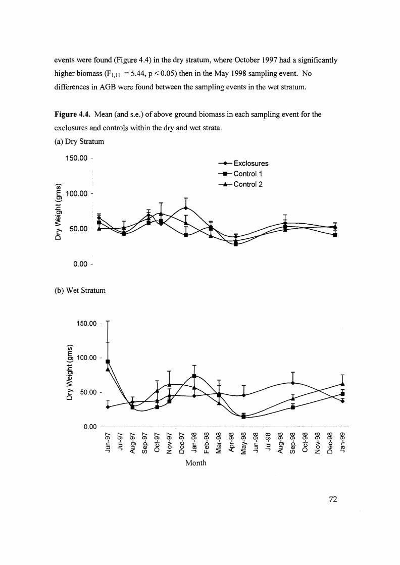
events were found (Figure 4.4) in the dry stratum, where October 1997 had a significantly
higher biomass (F1,11 = 5.44, P < 0.05) then in the May 1998 sampling event. No
differences in AGB were found between the sampling'events in the wet stratum.
Figure 4.4. Mean (and s.e.) of above ground biomass in each sampling event for the
exclosures and controls within the dry and wet strata.
(a) Dry Stratum
150.00 --
..-...rn~ 100.00 -
"-...'
+-'..cC)
~>. 50.00 - a--~____~
Q
0.00 -
(b) Wet Stratum
-+- Exclosures
-.- Control 1
-.-Control 2
150.00 -
......-..en
§, 100.00 -'-'+-'..c:::C)
~~ 50.00-(5
0.00 --------'-.-.--:-~---
f".. f".. ('0... ('0... ('0... ('0... ('0... co co ex:> co co co co CX) co co co co (j)(j) (j) 0'> m (J) 0> m 0'> en 0> 0> 0> 0> 0> 0> m (j) (J') 0> (j)
I ....!... I I I I I I I I I I I I I I I I I I
C C) a.. .., > u C .0 L.. ~ ~ c S 0> a. U > t.> C::J ::J
~Q) u 0 Q) ro Q) co
~ co ::J~
Q) 0 Q) coJ J
C/) 0 z 0 J LL ~ ~...., J
(f) 0 z 0 J
Month
72

4.3.2.2. Below ground biomass
In total for all samples throughout the study period, 1.2 m3 of soil was sampled and 11.03
kg of BGM was collected for analysis. The average dried weight of BGM was 9.19 kg /
m3• Mean differences in BGB for the dry stratum was 9.1 kg m3 for the exclosure and 9.3
kg m3 for the controls, and for the wet stratum 6.2 kg m3 for the exclosures and 6.9 kg m3
for the controls. No significant differences were detected in biomass between the
exclosures and controls in either the dry and wet strata. No significant differences were
detected between the exclosure and control in any sampling event. There were
significant temporal variations between the sampling events (Figure 4.5). For the dry
stratum, January 99 had significantly (Fg,17 = 8.67, P < 0.01) higher BGB then June and
October 1997 and January, March, May and September 1998 had significantly higher
BGB than January 1998. For the wet stratum, January 1999 had significantly higher
BGB (Fg,17 = 8.67, P < 0.01) than all other sampling events after August 1997 and
September 1998 had significantly higher BGB than all other sampling events after
August 1997, except for January 1999.
4.3.3 Earthwonn Biomass
In total, for all exclosures and controls throughout the study period, 1.2 m3 of soil was
collected and 280.8 g of earthworm were extracted, averaging 0.23 kg m3. No significant
differences in earthworm biomass between the exclosures and controls were detected in
the dry stratum, a mean of 0.33 kg m3 within the exclosures compared with 0.32 kg m3 in
the controls (Table 4.1). For the wet stratum, a significantly (FS,I7 = 7.5, P < 0.05) higher
earthwonn biomass was detected in the controls (0.29 kg rn3) than in the exclosures (0.22
kg m3). No significant differences were detected between the exclosures and control
within any ofthe sampling events. The mean worm biomass varied significantly among
sampling events (Fg,17 = 45.44, P < 0.001) in the wet stratum (Figure 4.6) with March,
May and September 1998 and January 1999 having significantly higher earthworm
biomass than June August, October and November 1997 and January 1998. The last
three sampling events in 1998/99 recorded signijicantly higher wonn biomass then the
1997 sampling events.
73

Figure 4.5. Mean (and s.e) of below ground biomass (kg m3) for all exclosures and
controls within the dry and wet strata.
(a) Dry stratum
30 ~
~ Exclosures
25 -: _ Control 1
--.- Control 2~ 20-C>
..................
..cC>
-ij) 15 -S~o 10-
5 _.
o -
(b) Wet stratum
30 -
25 --
'Ci 20 -.............0+00#
~0)
"Ci) 15-S>..L...
o 10 -
0 ._-~~~--~._~~--~._~---~~------ -~-~._ ......----~----------~----~&._....----.-- ....-_._--~~---~~.~-~............-.-~ .............~-~.~--~ ....~.~ .. __ ..--_.~----...........,-------
,...... f'- f'- f'... f'... ,...... I"- a;) a;) co co co co ex> co co co co ex:> 0'>(J) (j) en 0> (J') C'> (J) (J) 0> C'> m 0> (J) (J) en en (j) Q') Q') 0)
I I I I ..1 I I I I I I I I I I I I I I I
C 0) c.. > c.:> C .0 .... '- >.. c:: 0> c.. ....., > (.) c~ (.) ra~
~ (.)~ --;)
~<D 0 0 Q) ctS Q) co :J J ~
(1)0 0 OJ C'C
J (J) Z 0 J U. :2: :;: J (f) Z 0 --;)
Month
74
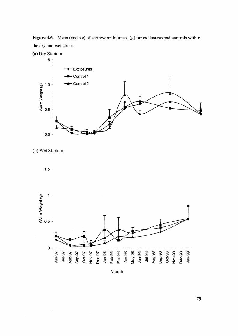
Figure 4.6. Mean (and s.e) ofearthwonn biomass (g) for exclosures and controls within
the dry and wet strata.
(a) Dry Stratum1.5 -
§ 1.0 ~
:EC>
~E....o .S 0.5 ~
0.0 ~
-+- Exclosures
-Control 1
-&- Control 2
(b) Wet Stratum
1.5 -
- 1 ~S.......c.0)
~E....oS 0.5 -
o -.~--- ~------~-~~~-----~-~~~--~---~
f'.. f'.. f'.. f'.. f'.. I"'- ........ co co co co co co co co co co co co (J)(J) (J) m en en en en (J) en m (J') m en en (j) m en m m en
I ....!.. I I I I I I I I I I I I I I I :> I I
C C> c.. t5 > (,) C .0 ..... ..... >. c "'5 C> Q. t) (,) C:J ::J
~Q) 0 Q) ro Q) co
~ co :J~
CD 0 (1) ro-, J en 0 z Cl -, u. ~ :2 -, -,en 0 z 0 -,
Month
75

4.3.4. Soil Moisture
No significant differences were detected between soil moisture levels in the exclosures
compared to the controls in either stratum. Temporal trends in soil moisture levels are
shown in Figure 4.7. High levels were reported after Cyclone Justin in the June 1997
sample and again after Cyclone Sid in February 1998. The average soil moisture content
was 19.9 % for the dry stratum and 32.6 % for the wet stratum.
Figure 4.7. Mean (and s.e) soil moisture content (%) for all exclosures and controls
within the dry and wet strata.
45 ~
40 -
35 ~
- :C 30 ~C~ 25 -o()
~ 20··.a 'en'0 15 2
10 '~
5 -
.......-Ory
_Wet
0·':------·---,-,--.
...... ,..... r--- r--- ...... ...... ,..... co co co IX) co co co co co co co co en0) a;> en 0) q> 0) q> 0'> 0'> (j) O? q> 0) q> (j) a> ~ q> q> (j)
C "3 0, 6- 0 >- (,) C ..6 Io!.. 0- >. C "3 C, c.. t> > (,). C:::J :::J Q) 0 Q) en Q) en en ::J ::J Q) 0 Q) en-;
...,« en 0 z 0 -; u. ~ « ~
..., -; « en 0 z 0 ...,Month
4.3.5. Interaction of measured ecological variables
A correlation matrix was derived for all variables (Table 4.3). Significant correlations
were detected between some variables within both strata. For the dry stratum, the
number of seedlings was negatively correlated with the seedling death rate and above
ground biomass, while positively correlated with seedling genninations, below ground
biomass and earthworm biomass. Above ground biomass was positively correlated with
seedling germinations and negatively correlated with alive seedling numbers, earthworm
biomass and soil moisture levels. Earthworm biomass was positively correlated with
seedling numbers, seedling germinations and soil moisture levels. Soil moisture levels
76

were positively correlated with seedling genninations and earthwonn biomass and
negatively correlated with above ground biomass. For the wet stratum, the seedling
numbers were negatively correlated with death rate and positively correlated with
seedling genninations and earthwonn biomass. Seedling germination was correlated with
seedling numbers and earthwonn biomass. Above ground biomass was not correlated
with any ecological variable while below ground biomass was correlated with earthwonn
biomass. Soil moisture levels were correlate~ with seedling death rate and earthwonn
biomass.
Table 4.3. Correlation matrix for all measured ecological variables within the dry and
wet strata. (* = Significant correlation value).
Strata Variables Variables
Alive Died Germinate AGB BGB Earthworm Moisture
Dry Alive 1.0Died -0.33* 1.0Germinate 0.54* 0.01 1.0AGB -0.25* 0.05 -0.22* 1.0-BGB 0.22* -0.02 -0.06 -0.08 1.0Earthworm 0.26* 0.12 0.33* -0.25* 0.14 1.0Moisture 0.04 0.13 0.22* -0.20* 0.01 0.43* 1.0
Wet Alive 1.0Died -0.26* 1.0Germinated 0.53* -0.03 1.0AGB 0.02 0.09 -0.08 1.0BGB -0.12 0.02 -0.02 0.1 I 1.0Earthworm 0.32* -0.04 0.23* 0.06 0.28* 1.0Moisture 0.03 0.18* 0.08 -0.06 0.11 0.17* 1.0
77

4.4 Discussion
The impacts that feral pig diggings have on the ecological processes within rainforests are
difficult to quantify. The rainforest ecosystem is complex and, in relation to the pace of
ecological systems, only a limited time scale was available for this study. However,
quantifying the impacts on the selected ecological variables in this ecosystem may
indicate what overall impacts feral pigs are having on the broad ecological processes
involved in this rainforest environment.
In overall terms, a mean of 31 % more seedlings were alive within the protected
exclosures, wet and dry strata combined, than in the unprotected controls. However, this
overall result was not statistically significant due to the inherent natural variability of
seedling numbers between the sites and exclosure replications. There was however, a
general trend of more seedlings surviving in the protected exclosures. Four of the six
exclosure in the dry stratum and, five of the six exclosures in the wet stratum had a higher
mean number of seedlings in the exclosures than in the controls.
There is also a positive trend over time of increasing seedling survival when protected
from pig diggings. The exclosures were established specifically to examine the recovery
ofthe ecological variables after protection from further pig diggings. If there was a
recovery effect then this recovery would be expected to be greater with increasing
protection time. Over the 2 year study, the mean number of seedlings within the protected
exclosures increased 7%, while the number in the controls decreased 37%. The difference
in seedling numbers between the exclosures and controls was influenced by the time of
sampling events. This was pronounced in the dry stratum where a significant interaction
affect was found. Significantly more seedlings were found in the exclosures compared to
the controls in the last three sampling events, the last 8 months of the study. The results
demonstrate that seedling numbers will recover when protected from pig diggings.
Recovery of gennination rates were also found within the protected exclosures in the dry
stratum, significantly higher rates ofgermination were found within the exclosures
compared to the controls in these last 3 sampling events. When comparing the first and
78

last sampling event in this dry stratum, the mean number of seedlings within the
exclosures had doubled while the seedling numbers in the control had remained relatively
unchanged. The recovery of germination rates was not observed in the wet stratum.
The dry stratum consistently recorded more seedlings in both the exclosures and controls
combined, compared to the wet stratum. The consistently higher than Donnal rainfall
during the 1998 dry season would tend to benefit the drier stratum, which usually has
very low soil moisture levels during the dry season, while conversely this abnonnal
rainfall would be detrimental to the wet strata due to soil saturation. Cyclones Justin and
Sid drowned many seedlings in the wet stratum; over 60% of seedlings died immediately
after cyclone Justin (March 1997). Seedling numbers were slowly recovering when
Cyclone Sid (January 1998) again caused over 50% of seedling to die. Continuing higher
then average monthly rainfall for 1998 kept pennanent water in the wet stratum, which
appeared to suppress germination and maintained a low number of seedlings. The
recovery of seedling numbers in the wet strata for 1998 were so affected by. saturated
soils that the effect of pig diggings was obscured.
This higher than normal rainfall for 1998 had the opposite effect in the dry stratum. The
higher then nonnal soil moisture levels throughout the 1998 dry season caused a high
number of seedlings within the exclosures to survive. However, this effect was only
found within the exclosures, the lower seedling numbers in the controls must have been
directly caused by the impact of pig diggings. The peak in diggings were found in the
May to July 1998 period (see figure 3.2, Chapter 3), so pigs were likely to be digging
within the controls at this time. It can be concluded that pig diggings were having a
direct impact on seedling survival in all of the controls by destroying germinating
seedlings during this 1998 dry season.
Pig diggings was also suspected to have an impact on the more mature seedlings. These
established seedlings are less vulnerable to normal seedling death factors, only 10% to
18% died due to natural factors as recorded inside the exclosures where there was no
diggings. Overall, 36% (27% in the dry and 440/0 in the wet strata) more established
79

seedlings died in the unprotected controls compared to the protected exclosures. This
result was not statistically significant so higher deaths in the controls could not be
directly attributed to the effects of pig diggings.
Ralph and Maxwell (1984) found in Hawaii that pig diggings significantly reduced the
volume of plants under 10 em in height (seedlings). Australian studies also support this
perception that pig diggings destroy seedlings (Alexiou 1983; Hone 1998). Bratton
(1975) in the USA, found pig diggings reduced under store cover by 85% to 92% and
significantly reduced the number of species present. Singer et al. (1984), also in the USA,
found an 80% reduction of vegetative cover in diggings compared to undisturbed
vegetation. Mack (1998) suggested that a "natural" level of physical disturbance of
seedlings in Papuan rainforests (without pig diggings) was 35% / annum. In comparison,
this study recorded a two-year natural seedling disturbance in the exclosures (where the
pig effect was removed), of 34.20/0 in the dry and 70.7% in the wet stratum, a mean of
58.2%.
Litter biomass remained relatively constant between the exclosures and controls.
However, litter biomass did fluctuate between sampling events due to seasonal effects.
The peak of litter biomass occurred at the start of the wet season agreeing with Brasell
and Sinclair (1983). This contrasts with Singer et al. (1984) who found a 51 % increase in
leafy litter inside an exclosure after 3 years; the depth and weight of leafy material was
65% and 59% lower respectively in intensive pig diggings. Pigs were observed in the
controls incorporating surface litter within the soil by their digging actions. However, no
clear indication that pig diggings had an impact on litter biomass could be derived from
this study.
No significant effect of pig diggings on the amount of subsurface plant biomass was
detected in this study. Incorporating litter by the pig's digging action in the controls did
not appear to translate into increasing below ground biomass. Below ground biomass in
both strata did show an increasing trend in 1998, in both the exclosures and controls,
possibly due to the above average rainfall throughout this year. However, no significant
80

differences in BGB were detected between the exclosures and the controls. This result
was inconsistent with the study by Lacki and Lancia (1983) who found significantly
higher organic matter levels in soil subjected to high intensity and frequency of pig
diggings. They suggested that the longer the area was affected by diggings then the
greater the change in soil organic matter. This incorporation oforganic matter into the
soil profile by digging enhanced the decomposition rate and expedited nutrient cycling.
The influence of the higher than nonnal rainfall in 1998 was also evident in the trend in
earthwonn populations. Both strata showed increasing earthwonn biomass during 1998
although the biomass was declining at the end of the dry season in the dry stratum. Both
strata showed consistent seasonal variations in earthwonn biomass between the
exclosures and controls. The influence of pig diggings on earthwonn populations was
positive in the wet stratum; more earthworms were in the controls than in the exclosures.
The digging action may have dried out portions of the soil (from saturation), allowing
earthworms cocoons to hatch. Alternatively, heaping of the soil by pigs digging action
may have allowed portions of the soil to drain, again allowing earthworm populations to
survive by oxygenating the soiL Earthworm biomass was slightly higher in the dry
stratum, possibly due to soil moisture saturation in the wet stratum. Pavlov et al. (1992)
found a reduction of earthworm populations in diggings compared to undisturbed soils,
although this was not confirmed by Mitchell (1993).
The recorded rainfall variation from "normal" values may have confounded the influence
of pig activity on seedling germinations and survivaL Longer research time frames and
more extensive sampling !!lay be required to overcome the influence of high levels of
seedling variability shown in this study. Twelve exclosure treatments may have been
insufficient to examine the impacts of pig diggings when the effects of natural variations
was so high.
Pig diggings appear to have no or limited impact on the amount of litter, root mass,
earthwonn populations, or soil moisture levels in this Wet Tropics study site. A true
quantitative assessment of pig diggings on seedlings however was more difficult to
81

obtain. The loss of 31 % of seedlings due to pig diggings may be ecologically
insignificant, the majority of these seedlings may have died anyway due to normal
attrition through predation from native species or competition for resources.
Feral pigs appear to have a direct influence on seedling survival in the drier
microhabitats. However, the confounding influence of the abnonnal rainfall in 1998 was
difficult to qualify and may have diffused the results. Also the limited time frame of this
study made it difficult to detect any long term ecological trends.
82

Chapter 5
Feral Pig Movements
5.1 Introduction
An important requirement for effective feral pig management is to obtain infonnation
on aspects of pig ecology in particular quantifying their movements, home range sizes
and migration patterns (Giles 1980, Saunders and Kay 1991). Auld and Tisdell
(1986) stated "In order to improve control procedures much more work is needed in
Australia to map patterns of movements of feral pigs, to more precisely determine
factors influencing such movements and to specify limits or barriers to such
movements". Knowledge of temporal and spatial home range areas and locations and
migration patterns are particularly important for effective management techniques to
be implemented. The area over which control operations should be applied and the
timing of control efforts to maximise effectiveness can be determined ifhome range
parameters and movement patterns are quantified (Caley 1997). Effective targeting of
control efforts in locations where pigs are known to concentrate will reduce control
costs and increase control effectiveness. Information on home range area is required
to identify the scope of the control operation, and appropriate control techniques
(Wood and Brenneman 1980).
The rainforests of the Wet Tropics are perceived to be the refuge of feral pigs (Pavlov
et al. 1992; McIlroy 1993; Mitchell and Mayer 1997). There is a perception among
the rural community that pigs live and breed in the WHA rainforest environment,
venture out to raid agricultural crops and then return to the protection of the rainforest
(WTMA surveys and media statements). Many landholders also have the view that
there are more pigs in the lowlands during the dry season than in the wet season
(Mitchell 1993). This has led to a perception of a seasonal migration of pigs from the
highlands to the lowlands in the dry season and subsequent return migration from the
lowlands to the highlands during the wet season. No scientific data exist to support
this perception.
No studies have been undertaken to quantify the movements of pigs within the Wet
Tropics region. Relevant studies have been undertaken in the wet/dry tropics in the
Northern Territory ,and in NSW and in the ACT (McIlroy and Saillard 1989; Saunders
83

and Kay 1991; Caley 1997; Dexter 1999). A number of studies have also examined
home ranges in mainland USA and Hawaii (Kurz and Marchinton 1972; Wood and
Brenneman 1980; Singer et ale 1981; Diong 1982b; Baber and Coblentz 1986;
Coblentz and Baber 1987).
Two aspects ofmovements ofpig were examined in this study. Firstly, long distance
dispersal or altitudinal movements (migration) that are perceived to occur in relation
to seasonal influences. The hypothesis that individual pigs move between the lowland
and highland habitats in response to seasonal influences was tested. Secondly, small
scale localised home range movement patterns were examined. The hypothesis that
the extent and distribution of home range movements is influenced by the seasons and
the sex of the animal was tested. These two aspects of pig movements were examined
separately (with some overlap) and are discussed below.
5.2 Methods
Radio tracking studies commenced in October 1994 and continued until February
1999. Within the three study areas (described in chapter 2), 22 male and 19 female
(n = 41) adult pigs (>24 months of age) were captured, fitted with radio collars and
released. Twelve pigs were subsequently deleted from the analysis due to insufficient
data. Of these, two pigs lost their collars, one died within 1 day of release, seven were
caught by hunters and two were in areas where their radio signals were masked by
radio interference. Of the 29 pigs that provided data (15 males and 14 females) all
contributed data to the migration movement analysis, while eight had a sufficient
number of known locations to be utilised in the seasonal home range analysis.
Pigs were captured in "box" and "silo" cage traps fitted with one-way doors (Allen
1984) and baited with waste bananas. Selected captured pigs were sedated for animal
welfare and safety reasons. Rompun (Xylazine Hydrochloride), a sedative analgesic
muscle relaxant, was injected intermuscular (2 - 3 mL of a 50 mg mL-1 solution) at
2.5-mg kg- l live weight; dosage was calculated from visual estimation of live weight
(Baber and Coblentz 1986). When the pig showed signs ofuncoordination, usually
within 5 to 10 minutes, a second intermuscular injection of Ketamine 100 ®
(ketamine hydrochloride,lOO mg mL-1) was injected at the rate of3.0 mg kg- l live
84

weight. A "jab" stick was used to inject the sedatives. In some situations pigs were
drafted into a small catch box and injected with a hand held syringe.
The combination of drugs rendered the pig semi conscious within 10 to 15 minutes.
The animals were then restrained with ropes around the legs anq around the upper jaw
be'hind the canines to prevent the pig from biting. One researcher would then hold the
pig while the other performed all the required tasks. Each selected animal was sexed,
weighed, aged by tooth eruption patterns (Brisbin et al. 1977, Clarke et al. 1992),
photographed, measured and a numbered plastic ear tag (Leader - Aussie Pig Tags)
inserted in one ear for future identification purposes. A radio transmitter collar was
then secured finnly around the neck of adult pigs. Due to the difficulty of recapturing
pigs in remote locations, only limited opportunity to re-catch and adjust collars was
available, so only adult pigs that had completed growth were collared to avoid
strangulation. Collars were supplied by "Sirtrack". Transmitter frequencies were in
the 150 to 152 MHz range and battery life for each collar was approximately 18
months. All pigs were left for 1 month after collaring before radio tracking
commenced to allow the animal to get used to the collar and resume nonnal
behaviour.
Location fixes were obtained by taking bearings to each radio collared pig from
"stations" which were marked locations of known coordinates. S~ations were located
on hilltops, forestry fire look-out towers, water towers, scenic lookouts and at easily
locatable positions identifiable on a map. Bearings from three to five stations were
obtained for each fix for each pig where possible, to enable triangulation of the pig
location and to establish the area of the bearing error ellipse polygon. When pigs
were located very close to stations, only two bearings were required as the location
error would be very small (White and Garrott 1990). In cases where only two bearings
were obtained, no error ellipse calculation was possible. Bearings were obtained
using a portable scanning receiver (Telonics - Telemetry Electronic Consultants,
Arizona, USA.) and standard three or four element "Yagi" aerials either mounted on a
tower in the back of a vehicle or held in the hand. Bearings were obtained using the
null - peak system (Saunders and Kay 1991). The magnetic bearing of the maximum
signal strength to the transmitting collar was obtained by bisecting the angle between
85

the two bearings (each side of the estimated strongest signal) where signal strength
dropped to zero (null).
As only one observer was available at each bearing fix, simultaneous bearings could
not be obtained. The technique used was to drive to different stations until a signal
and bearing fix was obtained, and then rapidly drive to other stations to obtain cross
bearings. The time between fixes was minimised as much as possible, varying from a
minute to a maximum of 10 minutes. Some movement between fixes was possible,
however in most cases location fixes were obtained within a few minutes of each
other. Stations were selected that were as close to the animals estimated position as
possible and at acute angles to the original bearing to reduce location error (White and
Garrott 1990).
The position of each pig was estimated using the computer program "Locate II" after
each bearing was corrected for magnetic deviation (8°). Location fixes were the
centre point of a 95% error eclipse. Bearing angle and location error were estimated
using the Lenth maximum likelihood estimator as described in White and Garrott
(1990). Location fixes were scrutinised for outliers based on field notes on signal
strengths and the animals estimated distances from the stations. Observers were
trained prior to recording data by locating collars attached to wooden pegs in locations
unknown to the observers. This method provided an estimate of bearing error for
each observer.
5.2.1 Analysis of migration movements.
The hypothesis that individual pigs migrate between the lowland and highland
habitats in response to seasonal influences was examined. An annual (combined wet
and dry season) home range area was calculated for each radio collared pig in each of
the three areas. An observed movement from one area to another would be
considered as a migration movement. Movement distances from their home range
centre that were greater then twice the mean diameter of the calculated home ranges,
were defined as a migration movement.
Migration patterns were determined by obtaining periodic fixes on radio collared pigs
over the battery life of the collar (12 to 18 months). All 29 collared pigs were used in
86

the analysis, seven in the highland area (3 male, 4 female), 10 in the transitional area
(5 male, 5 female) and 12 in the lowland area (7 male, 5 female). A location fix was
attempted at least once per month, on average 2 to 3 times per month. In reality, fixes
were obtained on an opportunistic basis, whenever the observers were within the
areas. Cyclones, restricted access due to weather conditions and landslides, and the
thick vegetation restricting signal strength, all combined to make accurate periodic
positional fixes on pigs in remote mountain locations in the highlands difficult to
obtain.
When pigs with known active collars could not be located, an aerial search was
initiated. Aerials were attached to the wings of a Cessna 207 fixed wing light aircraft
and flown over the last known location of the missing pigs. If a signal was detected,
the relative signal strength from the two aerials was used to direct the plane towards
the signal. The pig location was estimated using the method of White and Garrott
(1990) whereby the plane flies in a decreasing circle keeping the strongest signal on
the wing aerial facing the pig. The pig position was estimated from a combination of
signal strength and the centre of the flight circle. Coordinates were obtained from
visual interpretations of maps. No location error was calculated, as this was not
critical to the aims of the study.
Location data were analysed using the Ranges V program. Home range estimates
were derived from the "minimum convex polygon" (MCP) analysis. This method is
strongly influenced by peripheral fixes, so a peeled polygon analysis based on 95% of
range fixes was used to eliminate the outermost 50/0 of fixes. This MCP analysis is the
most common method of estimating home ranges due to its simplicity, ease of
calculation and robustness with a low number of fixes (White and Garrott 1990). The
harmonic mean fix estimate (Hc) for each pig was calculated to estimate the centre of
range activity (hannonic centre), the maximum range span distance and the mean
distances affixes from the calculated He (Dixon and Chapman 1980). This method
calculated the mean distances that pigs moved from the home range centre.
5.2.2 Analysis of seasonal home ranges.
Seasonal home range calculations were required to examine the extent and
distribution ofpigs in relation to seasonal influences. The hypothesis that the size of'
87

the home range and changes in their centre of activity are influenced by the sex of the
pig and by the effects of the wet and dry seasons were examined.
Field techniques to collect location fix data to calculate home range movements on a
seasonal basis in the highlands of the WHA were not practical. Ground telemetry
methods were limited as radio signals could not penetrate more than 2 Ian through the
thick vegetation and limited access prevented the observers from approaching close
enough to the collared pigs to receive accurate signals. Accurate and multiple
periodic location fixes of collared pigs were required to calculate seasonal home
ranges so seasonal home range estimations were obtained only from location fixes of
pigs in the transitional and lowland areas (Figure 5.1.). Sufficient numbers of location
fixes in each season to enable accurate seasonal home range estimations to be
calculated could not be obtained for all pigs. Only two pigs (lmale and 1 female) in
the lowland area and six pigs (3 males and 3 females) in the transitional area had
sufficient location fixes (within a d~fined season) for seasonal home range
calculations.
Locations were calculated from ground telemetry methods described above using two
observers. Location fixes for each season were obtained over three 72-hour tracking
sessions. During each session, fixes were obtained at three hourly intervals (stann
activity and flooding prevented some location fixes from being obtained),
commencing at 0900 hours for the first 24 hours, 1000 hours for the next 24 hours and
1100 hours for the last 24-hour tracking period. Thus over the' 72-hour sessions, 24
location fixes for each pig were attempted, corresponding to a fix location for each
hour of the day. Location sessions were then repeated three times over three
continuous weeks in the dry season (November), and the procedure was repeated in
the wet season (February). Due to the time difference between obtaining bearings
(range of 1 to 10 minutes), bearings for each pig were obtained in the same order for
each tracking session to keep time differences between fixes for each individual·pig
constant. Aggregate and seasonal home range area estimations were calculated as
above using the 95%"minimum convex polygon" (MCP) method (White and Garrott
1990). Increment area plots were examined to see how the home range area changed
as successive location fixes were added. This was used to test the relationship of
home range area (% ofrange area) with the cumulative numbers of fixes.
88


Sufficient number of fixes to accurately estimate the home range occurred when this
relationship plot reached an asymptote. Only pigs that reached an asymptote were
used in home range estimations. The effects of seasons and sex on home range areas
were examined by 2 way ANOVA. The hannonic mean fix for each home range
within each season was calculated to examine if a shift in home range centres
occurred in response to changing seasons.
5.3 Results
5.3.1 Location Error
Error estimations were calculated for the seasonal home range study only. The
problem of obtaining multiple bearings (three are required for error calculations) and
aerial fixes for pigs in remote areas prevented error estimations for pigs used in the
migration movement study. Estimations of error obtained were used to represent all
triangulation calculations (Table 5.1).
The overall mean bearing error angle for 238 location fixes obtained from seven pigs
was 3.08° (95% C.I. = 6.16°), the mean area of the 95% error ellipse around 229
location fixes was 10.17 ha. The mean location error was 68 m (maximum 136 m) at
1 kIn from the antenna. As most fixes were estimated to be less then 1 kIn from the
location stations, this error was considered small enough for the aims of this study.
5.3.2 Migration Movements
In total, 29 pigs (15 males and 14 females) were used to examine migration
movements. These were seven (3 males, 4 females) in the highland area, ten (5 males,
5 females) in the transitional area and twelve (7 males, 5 females) in the lowland area.
No pigs were located outside their initial area of capture at any time during the study.
No movements in relation to the altitudinal gradient between the lowland area and
highland area was observed for any collared pigs. The outline of calculated home
ranges for all pigs examined in this study are presented in Figure 5.2. A feature of
this study is the extensive overlap of individual home range boundaries.
90-

~I
D

Table 5.1. Estimated 95% error ellipse area (ha and s.e), bearing angle (0) error and
number (n) of fixes used in error calculations for each pig. (* - not calculated).
Season Sex Pig Fixes Mean Area (ha) Bearing Angle
I.D. (n) 95 % Error Ellipse (s.e.) Error
Dry M Nigel 24 7.72 (1.47) 2.91
M Peter 20 8.34 (2.39) 3.09
M Sleepy 25 11.13 (2.74) 3.08
M Steve 23 20.7 (6.2) *
F Kennedy 29 8.67 (1.65) 2.89
F Blondie 9 10.07 (2.85) 3.32
F Vicky 33 6.8 (1.6) *Wet M Nigel 3 7.15 (6.41) 2.67
M Peter 18 12.33 (2.34) 3.5
M Sleepy 25 7.24 (1.75) 2.69
F Kennedy 11 9.23 (2.22) 2.8
F Cathy 9 11.87 (1.95) 3.45
F Blondie 9 11.02(4.04) 3.5
Location fixes in both the wet and dry seasons for each collared pig were used to
calculate their annual home range size .and the distances that the pigs moved from
their calculated home range hannonic centre. In total, 940 location fixes were
calculated (Table 5.2). Each individual pig had a mean of34 location fixes (range 6
137) for a mean tracking .period of 13.14 months (2.5 location fixes /pig / month).
92

Table 5.2. Home ranges areas (km2) and movement distance from the Harmonic
Mean Centre (Hc) for all pigs within the three areas. The total time of tracking
(months) and number of fixes derived for each pig are also given.
Area Pig Sex Tracking Number Home Mean Distance (km)ID. Time of Fixes Ran~e From Hannonic Mean
(Months) (n) (km ) Centre (He)Range Mean Max
Highland RICHARD M 10 11 4.61 1.94 0.73 1.78SMOKO M 10 9 3.84 1.73 0.63 1.49SID M 8 8 6.0 2.24 0.72 2.06RHANE F 14 13 10.06 4.41 1.8 4.4JULIANNE F 20 12 9.71 3.26 1.09 1.94SIS F 14 11 9.55 4.14 1.72 3.27GUNNA F 17 6 6.57 2.97 1.07 2.88
Transitional DAVE M 13 7 6.79 2.97 0.88 2.68BALLS M 7 11 2.85 1.21 0.36 0.76NIGEL M 6 84 21.21 6.1 1.1 3.84PETER M 6 132 4.89 4.9 0.75 3.1SLEEPY M 6 137 4.75 3.77 0.8 2.8BRONX 2 F 17 7 3.25 1.27 0.34 0.64BRONX 1 F 18 14 7.18 3.07 0.92 2.42KENNEDY F 6 119 3.09 4.48 0.6 2.8CATHY F 6 44 3.7 2.98 0.88 2.0BLONDIE F ·6 69 4.53 3.76 0.97 2.4
Lowland IMPERIAL M 22 20 15.39 4.4 1.6 2.8DUCK M 19 8 3.97 1.44 0.5 0.99DART M 18 10 4'.1 1.5 0.67 1.2STEVE M 16 65 9.96 5.87 0.74 4.78DAL M 12 13 4.5 1.7 0.57 2.77COROLLA M 8 8 4.92 3.6 1.2 2.98METRIC M 33 20 33.14 11.6 5.8 11.5112 F 13 14 10.1 3.35 1.29 2.68787 F 10 26 5.86 3.05 0.77 2.7SALT F 15 9 4.23 1.67 0.98 1.64VICKY F 17 78 13.07 3.9 1 2.787 F 14 29 9.34 3.78 0.89 2.49
93

Due to the large variation in the number of fixes used to derive the individual home
ranges (range 6 to 137), the relationship of the number affixes and the derived home
range area was examined (Figure 5.3). A Kruskal-Wallis one way ANOVA on ranks
test found no significant relationship could be detected (p = 0.16). No significant
changes in home range area were detected between pigs with low number of fixes and
pigs with high number of location fixes. Subsequently all home range estimations
were combined for analysis.
Figure 5.3. Relationship of home range area and number of location fixes used to
derive the home range estimate. Regression line is shown.
35 -•
160140
• ••120
y =0.0031x + 7.8665
R2 = 0.0004
•
•
••
60 80 100Number of Location Fixes
•
40
•
30 ~
Ng25 -Q)N
i:i5 20 -Q)C>
ffi 15 -: •c:::(])E 10 _. fill'~ -....--..~--------------------
5 ~ Jr ·o _.~---- ~...,....---~
o 20
No significant differences in home range areas in the three areas combined were
found between males and females (F 1, 28 = 0.066, P = 0.8). Males had a mean home
range area of 7.92 km2 (s.e = 1.79) and females 7.28 km2 (s.e. = 1.75) (Table 5.3). No
significant differences in home range sizes (male and female combined) were found
between the three areas (F2, 28 = 0.85; P = 0.44). The interaction of sex and area was
not significant (F2,28 = 0.81; p = 0.46). The overall mean home range for all pigs in
all areas was 7.57 km2 ± 2.43 km2 (s.e. = 1.19).
94

Table 5.3. Mean home range for male and female pigs (n) in the three areas. (Home
range estimated by the 95% MCP method).
Area Male Home Range (n) Female Home Range (n)
km2 (s.e) km2 (s.e)
Highland 4.82 (3.77) 3 8.97 (3.26) 4
Transitional 8.1 (2.92) 5 4.35 (2.92) 5
Lowland 10.85 (2.47) 7 8.52 (2.92) 5
The average and maximum distances pigs moved from their centre of activity
(hannonic mean fix of the home range) are presented in Table 5.4. The mean distance
any pig in any area moved from their hannonie mean fix was 1.03 km; the mean
maximum distance any pig moved from the He was 2.64 km.
Table 5.4. The mean and maximum distance (km) males and females moved from
the hannonic mean fix (Hc) of their home range within the three areas.
Area Distances from He Distance from Hc
Male Female
Mean Max Mean Max
Highland 0.69 1.78 1.42 3.13
Transitional 0.78 2.64 0.74 2.05
Lowland 1.58 3.86 0.99 2.38
5.3.3 Seasonal Home Range Study
In total, 669 location fixes (359 in the dry season and 310 in the wet season) were
obtained for eight pigs (4 males and 4 females). The calculated home range sizes for
all pigs for both seasons is presented in Table 5.5. Mean home ranges for the dry
season were 9.78 km2 (s.e. = 4.85) for males and 4.89 km2 (s.e = 1.27) for females.
For the wet season mean home range for males were 2.76km2 (s.e. = 0.34) and
females 3.02km2 (s.e. = 0.56) (Figure 5.4). A 2 way ANOVA found significant
seasonal effects (F 1,12 = 5.59; p < 0.05), non-significant difference between the sexes
(F1,12 = 0.44; P = 0.52), and a non-significant season x sex interaction (F1,12 = 0.77; P
= 0.4).
95

Table 5.5 Home Range estimations (95% MCP) for male and female pigs for the wet
and dry seasons.
Season Sex Pig Fixes Home Range
Identification (n) (km2)
Dry M Nigel 36 24.3
M Peter 81 5.12
M Sleepy 75 4.27
M Steve 34 5.45
F Kennedy 65 3.0
F Blondie 20 4.36
F Vicky 48 7.31
Wet M Nigel 48 3.44
M Peter 51 2.45
M Sleepy 62 2.38
F Kennedy 56 1.9
F Kathy 44 3.7
F Blondie 49 3.48
For each season, results for male and females were pooled as no significant
differences between them were found. Home ranges in the dry season (7.69 km2)
were significantly greater (F 1,12 = 6.6; P < 0.05) than in the wet season (2.89 km2).
Males had an aggregate home range of 10.2 km2 (s.e. = 3.86) and females 6.1 km2 (s.e.
= 2.34) (Figure 5.2). There was no significant difference in aggregate home range
between males and females (F1,7 = 1.07; p> 0.05). The overall mean home range area
for all pigs in both seasons was 5.47 km2 ± 3.53 km2 (s.e. = 1.62 km2).
96

Figure 5.4. Mean home range size (km2 and s.e.) ofmale and females pigs within the
wet and dry season, and the aggregate home range for both seasons combined.
16 -:
14 ~
12 ~
E 10~ :
CDC)
~ 8~
c:::CD
~ 6'~J:
2 ~
oDry Season
ElMaie
o Female
Wet Season Aggregate
The harmonic mean fix for each home range within each season was plotted to
examine if home range centres moved between the seasons. The mean distance
between the Hc for each seasonal home range was 651 m (range 539m to 806m) for
males and 250 m (range 141m to 360m) for females. The outlines of home range
boundaries are presented in Figure 5.5.
97


5.4 Discussion
Two aspects of feral pig movement patterns within the WHA were investigated in this
study, large scale migration movement and small scale seasonal home range sizes. No
scale migration movements of the sampled pigs occurred during this study. Home
ranges sizes for both male and females were larger in the dry season compared to the
wet season. No difference in home range sizes were evident between male and female
pIgS.
5.4.1 Migration Movements.
No evidence of large scale migration type movement patterns of the collared feral pigs
were found in this study. Observed movements tended to be limited to within small
scale defined home range boundaries. No evidence of longer distance movements
over the altitudinal gradient (highlands and lowlands) that may be considered
migratory were found. No collared pig was observed to move outside the highland,
transitional or lowland area where they were initially captured. The mean distance
that pigs moved from their home range centre (harmonic mean fix) was slightly more
than 1 km, a distance well within normal home range movements. Home range sizes
were calculated over an average 13 month tracking period, so all pigs used in the
analysis had fix locations during the wet and dry seasons. The hypothesis of
migration occurring in relation to seasonal influences was not supported.
The absence of large scale migration movements within the region is consistent with
the results obtained from studies in other environments other. Caley (1997) found
from hunter returns, that pigs are relatively sedentary in the N.T., with a mean
recapture distance of 3.2 km for males and 1.8 km for females. He found that the
effect of time since initial capture on recapture distance was not significant, so no
long-term dispersal trend could be identified. Almost all of the male and female
recaptures (94% and 1000/0 respectively) were captured within the upper 95%
confidence interval of their home range diameter, that is the distance pigs moved from
their initial capture point could be explained by normal movements with a defined
home range. Giffin (1978) also found a recapture distance of 1.1 km for males and
1.4 for females in Hawaiian rainforests, all pigs were recaptured within their normal
home range boundaries, conforming to the results of this study.
99
Saunders (1988) and Hone (1988a) found significant seasonal altitudinal movement
in their studies that could be tenned migration movements. Pigs preferred higher
altitudes in summer and lower altitudes in winter. Temperature influences may be
responsible for this altitudinal movement; very cold temperatures (including snow)
that occur could force pigs to warmer lower altitudes. Singer et al~ (1981) also
reported seasonal changes in altitude preferences in the Great Smoky Mountains
National Park (USA), and attributed this to shifts in food availability, particularly the
seasonally abundant acorn crop. The lack of cold temperatures and the absence ofa
seasonally abundant natural food source occurring at different altitudes or seasons in
the Wet Tropics region may explain these contrasting results.
Hart (1979) found seasonal movements between habitats in his N.S.W. study. Pigs
concentrated in forestry areas around pennanent water sources during dry periods and
then moved to the coastal plains where food supplies were more abundant during wet
conditions. Bowman and McDonough (1991) found that pigs concentrated in swamp
communities during the dry season in the Northern Territory and moved into the open
plains and forests during the wet season. Caley (1997) found that pigs were
significantly associated with riparian forest vegetation throughout the year at a similar
site in the Northern Territory, but moved into cropping situations in the early to mid
dry season. Hone (1990b) found significant seasonal differences in density indices
within habitats in the Northern Territory. Pigs appeared to move between open
floodplains and swamps in response to seasonal flooding, but movements between
habit~tswithin each season appeared to be in response to food and water availability.
In overseas studies, changes in habitat usage have been attributed to rainfall and
temperature patterns (Malaya) (Diong 1973), food availability (USA) (Graves 1984;
Kurz and Marchinton 1972; Brisbin et ale 1977; Singer et ale 1981; Baber and
Coblentz 1986) and density of available cover (USA) (Barrett and Pine 1980).
Overseas studies have found larger movement distances for different pig species.
Diong (1973) found bearded pigs (Sus barba/us) in Malaysia with sugar cane in their
stomachs 8 to 16 kIn away from the nearest cane farm. In France, Dardaillon (1987)
found 40% of Eurasian wild boar (Sus scrofa scrofa) were recaptured 20 to 68 kIn
from the initial capture point, while Andrzejewski and Jezierski (1978) also reported
that five Eurasian wild boars moved 5 to 250 kIn from their study area.
100

Disturbances such as large scale hunting pressure or prolonged harassment may cause
shifts in the pigs home ranges (Caley 1993a). Giles (1980) reported a movement of
23 km for two boars in response to flooding, and Saunders and Bryant (1988) reported
a movement of 55 km for a sow during a major control operation. Small scale
disturbances generally cause pigs to temporarily shift home ranges but return after the
disturbance has subsided (McIlroy and Saillard 1989; Caley 1993; Choquenot et al.
1996). Anecdotal reports of large-scale movements in this study site may be due to
intense hunting pressure. Large identifiable males that cause considerable economic
damage to sugar cane and banana crops have frequently had a bounty placed on them.
The resultant intense hunting with dogs over a prolonged period may force these
males to relocate some distance away. Infonnation from landholders in the study site
suggests that hunters who target these large males invariably chase the males into new
locations; some reports of movements of up to 20 km away have been suggested.
Most landholders agree that in areas where hunting pressure is low, boars remain
sedentary and are often seen in the same location for many years. This anecdotal
information in some ways reinforces the results of this study (although not
specifically studied) that pigs are sedentary within defined home ranges when
undisturbed in the remote rainforest areas but react to disturbance in the transitional
and lowland areas by relocation to new more favourable home ranges.
Weather conditions, especially high temperatures, may cause a movement shift
between habitats to avoid high temperatures. Dexter (1998) showed that when
temperatures were high pig populations concentrated in s~ady habitats. However
food availability influenced habitat selection when temperature constraints were
relaxed. Dexter (1999) found a sex difference in home range areas, females
responded to changing environmental conditions while males did not. Females were
influenced by two of the same variables that influence habitat usage; daily maximum
air temperature and pasture biomass, suggesting that the factors governing habitat use
and home range sizes are not independent.
Individual behavioural factors may be additional considerations for defining home
range sizes with temperament and tolerance of human activity. Giving birth and
hunting pressure are also considerations in influencing home range area. Two of the
transitional females were known to have young at foot during the radio tracking
101

sessions, and hunting was observed on a number of occasions in the lowland and
transitional areas.
The variation of female home ranges sizes was in the order of400% (3.1 km2
minimum to 13.1 km2 maximum). Male home ranges size variation was in the order
of 1100% (2.9 km2 minimum to 33.1 km2 maximum). Two large males, Nigel in the
transitional area and Metric in the lowland area, were responsible for the largest home
range sizes, 21.2 km2 and 33.1 km2 respectively. Both of these males were over 100
kg in weight, were always solitary when able to be observed and displayed
disproportionate aggressive behaviour when captured. These boars could be
described as "loners" who perhaps have had limited contact with humans prior to
capture. In contrast, some ofthe pigs captured in the transitional area appeared to
tolerate human activity; their home ranges overlapped human activity zones such as
intensively fanned banana plantations. These pigs were. also less aggressive when
captured.
5.4.2. Seasonal Home Ranges
The overall mean aggregate home range area reported in this study of 10.2 km2
(males) and 6.1 km2 (females) are comparable with other Australian studiesw
Estimated horne ranges sizes vary from lw4 to 43 km2 for males and 1.5 to 19.4 km2
for females from a variety of habitats (Choquenot et al. 1996). Comparative home
range data derived from Australia and overseas studies are provided in Table lwl.
The home range sizes calculated in this study are similar to estimations in habitats
considered favourable to pig populations (Saunders 1988; McIlroy and Saillard 1989;
Dexter 1995). However, home range sizes within this study were generally smaller
then those estimated in habitats considered less favourable to pig populations (Giles
1980; Saunders 1988; Caley 1993a). Comparisons with overseas studies indicated
home range sizes in the Wet Tropics are generally larger (Diong 1982b) (Baber and
Coblentz 1986; Singer et al. 1981).
Males tended to have larger home range sizes than females in both the home range
and migration movement studies, but this difference was not statistically significantw
Indeed if the abnonnal large home range of Nigel is removed from the seasonal home
102

range analysis, male and female home range areas were almost identical (3.9 km2).
The migration study found only a 0.64 km2 difference in home range area between
males and females. Other studies have found that males have larger aggregate home
ranges then females (Barrett 1978; Giles 1980; Baber and Coblentz 1986; Saunders
1988; Saunders and Kay 1991; Caley 1997; Dexter 1999).
Lindstedt et al. (1986) linked home range area with the resource requirements dictated
by an animal's body mass. They argued that home range is a linear function of body
mass due to the rate of physiological and ecological processes being linked to body
mass; the larger the animal the more area it needed to forage in to find adequate food
resources (Baber and Coblentz 1986; Saunders 1988). Saunders and McLeod (1999)
suggested that males and females have identical home ranges areas, once the effects
of body mass are taken into account. This effect has also been found in feral pig
studies in central NSW (Giles 1980; Saunders and Kay 1996); USA (Singer et al.
1981; Baber and Coblentz 1986) and in tropical Australia (Caley 1997). Dexter
(1999) found that this influence on home range areas was apparant for female pigs but
not for males in semi arid NSW. He suggested that males needed to maintain a larger
home range to maximise their probability of encountering females, and that
reproductive success was more important than resource requirements.
In the Wet Tropics, availability of food and water appears to be abundant. This may
mask the influence of body mass on home range area. All resource requirements for
the observed larger body mass of the captured mature males (average 87 kg, n = 50)
may be available within the same area that the lower body mass females (average 57
kg, n = 43) occupy. The resource requirement interaction with body mass may not be
an influencing factor on home range size when resources are not a limiting factor.
Massei et al. (1997a) in a coastal Mediterranean study, supported this hypothesis
when they found there was no inverse relationship between food availability and
home range size contradicting the "food exploitation hypothesis". No differences in
home range sizes between males and female pigs were detected in their study.
In this Wet Tropics study, significant seasonal effects on home range sizes were
found, home range sizes were significantly larger in the dry season than in the wet.
The wet season is when fruit and water availability and distribution is maximised.
103

Pigs presumably do not have to move far to get their resource requirements in this
time of plenty. In the dry season, resource availability is possibly reduced and home
range size may have to increase to enable sufficient resources to be obtained. Other
factors may influence the size ofhome ranges in the Wet Tropics; age, sex,
physiological status, energetic requirements, population density and hunting pressure
(Massei et al. 1997b). The similarity of home range areas in suitable pig habitats
throughout Australia suggest that pigs limit their movements to the smallest home
range area where all resource requirements are met.
Home ranges for males and females were irregular in their configuration and
overlapped each other. This further suggests that resources are abundant in the WHA
as competition for limiting resources would cause individuals to defend resource sites
with a corresponding decrease in range overlap. Daily home ranges reported in other
studies (Saunders 1988; Caley 1997) suggest that pigs do not occupy their entire home
range over short periods, indicating they are not territorial.
Differences in geographical centres of home range between wet and dry season
averaged 651 m for males and 250 m for females in this study. In comparison
seasonal differences in summer and winter home range centres in Tennessee (USA)
average 6 kIn (n =13) (Singer et al. 1981). This supported the migration study
findings where distance between centres of home range activity was not significant.
104

Chapter 6
Demography of Feral Pigs
6.1. Introduction
Knowledge of the demography of pig populations is vital for modelling the mechanisms
underlying their ecology and rates of population change, as an aid in developing
management strategies. Knowledge of demography is also necessary for modelling
epidemiological calculations in exotic disease contingency planning. These two models
are of major importance to feral pig management within the Wet Tropics.
Major feral pig demographic studies have been conducted in the semi arid regions and
southern highlands ofN.S.W.(Giles 1980, Hone and Robards 1980, Saunders 1988,
Pavlov 1991, Saunders 1993a), in the N.T. (Caley 1993b, Caley 1997); and in New
Zealand (McIlroy 1989). 'No comparable demographic studies have been attempted in
the Wet Tropics rainforests.
Saunders (1993a) described demographics for feral pig populations in Kosciusko
National Park (N.S.W.) and compared his results -with other published studies (Giles
1980, Pavlov 1980, Caley 1993b). He suggested the substantial differences found in the
demography of pig populations he compared were a result of differences in
environmental factors between habitats. Population demography at Kosciusko N.P. was
characterised by a seasonal breeding pattern, with most births occurring in summer and
autumn due to reduced food availability in the winter. Giles (1980) found that pig
populations fluctuated markedly in response to seasonal conditions in semi arid N.S.W.,
primarily influenced by the availability of dietary protein as a response to rainfall,
especially flooding. Caley (1 993a) also found the demography of pigs in the NT was
influenced primarily by food availability which was correlated with rainfall. He also
suggested that the pig populations he studied were significantly influenced by the
presence of cropping systems.
The main influences on pig demography in the Wet Tropics are unknown. Seasonal
patterns of temperature and rainfall, seasonality of fruit fall, and other components of
the diet including the availability of dietary protein are all factors that may influence the
demography of pigs within the Wet Tropics. The aim of this study is to describe and
105

compare aspects of the demography of a trapped sample of pigs in the WHA with the
major published pig demography studies in Australia (Giles 1980, Saunders 1993a,
Caley 1993b). Limited data from overseas studies have also been provided for
comparative purposes.
6.2. Methods
A system of feral pig traps was established within the three areas described in Chapter
Two. Approximately 25 traps were used throughout the study site. Trapping was
conducted continuously from 1994 to 1999, except when periods of flooding, cyclones
and road closures restricted trapping activity within some areas. Feral pigs were
captured within all of the three study areas, however the majority of pigs were captured
within the lowland area. Restricted access due to cyclones and road closures and the
marked seasonality of trapping success restricted continuous trapping activity within the
highland area.
6.2.1. Trapping Techniques
Feral pigs were captured in box and silo cage traps described by Allen (1984). The
trapping strategy consisted of placing food material (bananas rejected for market), at
sites pigs were known to frequent from signs of diggings, or in preferred pig habitats
such as creek lines and swamps. When feeding activity commenced, traps were
positioned at the feeding sites with the doors wired open to entice pigs into the traps.
After three days of free feeding, the traps were set using a pig specific trip mechanism
to prevent capture of non-target species. Selected individuals used for other studies
were examined and releaseda All other captured pigs were humanely killed and
biological data (sex, age, weight, colour, and a range of morphological measurements)
were recordeda
6.2.2. Trapping success-effort assessment
A small scale trapping project was conducted concurrently with the trapping program to
estimate trapping success-effort rates. Two trapping systems were established; eight
traps in the highland area (Society Flats) and nine traps in the lowland area (Edmund
Kennedy National Park)a Traps were inspected daily after the initial bait material was
placed in the traps. The time (days) taken for pigs to find the bait and enter the trap,
time to first capture and number of pig captures were recorded.
106

6.2.3. Population Structure
All captured pigs were aged, in months, by the tooth eruption method described by
Clarke et ale (1992). No attempt was made to age pigs (in months) that were estimated
to be older than 36 months, as the molar wear index technique used in other studies is
un-calibrated for this region. All aged pigs were assigned to seven none overlapping
age categories i.e. less than 6 months, 6 to 11 months, 12 to 17 months, 18 to 23
months, 24 to 29.months, 30 to 36 months and 36 months and older. Difference in
capture frequencies between the sexes and age categories was tested by Chi Squared
analysis. The capture frequencies of the different age categories were plotted, to
extrapolate the maximum age of survival and to derive a relationship of age category
with capture frequency. A life table was constructed from the trapped sample as
described by Caughley (1977), with the trapped sample assumed to represent an
imaginary cohort. The frequency of the zero age category was calculated from the
number of mature females in the sample, multiped by the calculated mean litter size and
the estimated frequency of births.
6.2.4. Reproduction.
Captured adult females not released for radio tracking purposes were killed, autopsied
and examined for pregnancy. Foetuses (if present) were aged by the crown-rump
measurement method of Henry (1968). Foetal number and number of young at foot
(young trapped with a lactating female) were used to estimate litter size. The ages of
pigs less then 36 months were backdated to calculate their birth month. The mean date
and frequency of birth month were calculated using the method described by Caughley
(1977). The number of pregnant and/or lactating females was used to calculate a
fecundity schedule and the prevalence (P) ofpregnancy, the proportion of females
pregnant at a given time or reproductive success for each age category. The incidence
of pregnancy (I), the number of times an average female becomes pregnant during a
year was calculated from I = P / D where D is the time duration when pregnancy can be
visually detected, estimated to be 3 months using autopsy techniques (Caughley 1977).
6.2.5. Morphometric measurement
The following range of body measurements (em) were taken for all captured pigs.
107

(a) snout - tip of the snout to the centre point between the eyes
(b) head - tip of snout to nacha! crest
(c) total body - tip of snout to tail butt
(d) height - tip of front foot to top of the shoulder
(e) foot - tip of hind foot to point of the ankle.
All morphometric measurements were examined for sex differences by one - way
ANOVA. Body measurements were also examined for relationship with age by
regression curves fitted to the plotted data. An age estimation index was calculated for
each sampled pig by the method of Boreham (1981) where an Age index (I) is derived
from morphometric measurements by the equation:
I = (head length + total body length) / 2
The age index, calculated for males and females, was then compared to the estimated
age using tooth eruption teclmique. Choquenot and Saunders (1993) recalculated
Bareham's data and derived polynomial regression equations for male and female pigs
(to account for their differing gro\Vth patterns) directly relating the Boreham age index
(I) to age in days (A) i.e.
Males A = -5.019] + 0.140]2
Females A = -5707 I + 0.158]2
These equations were used to calculate a Choquenot age index from the calculated
Boreham's index (I) for all sampled pigs. Pigs more than 36 months of age or with a
calculated Boreham age index ofmore than 100 were excluded from the analysis.
Regression models were fitted to both age indices to test for differences in age
estimation from the two age index calculations with estimated age from tooth eruption
methods.
All pigs were weighed as live weight (kg). A regression analysis of the log transformed
weight / age and weight / body length relationship was calculated and plotted.
Comparisons of the calculated relationship were made with other published
morphometric studies. Saunders (1988) generated a model to predict body weight (kg)
from total body length i.e.
In body weight = -10.6 + 3.041n total body length
Data collected from the trapped sample were used to derive a relationship of body
weight with total body length and compared with the actual body weights recorded from
108
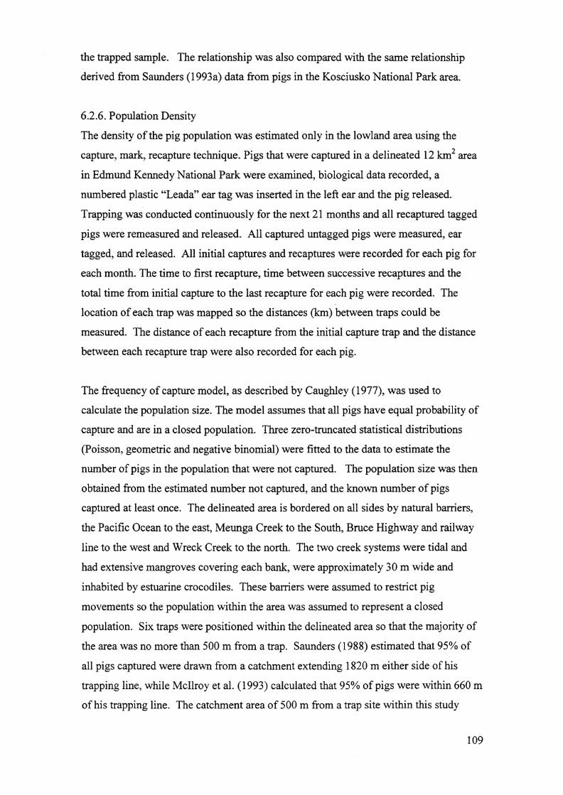
the trapped sample. The relationship was also compared with the same relationship
derived from Saunders (1993a) data from pigs in the Kosciusko National Park area.
6.2.6. Population Density
The density of the pig population was estimated only in the lowland area using the
capture, mark, recapture technique. Pigs that were captured in a delineated 12 km2 area
in Edmund Kennedy National Park were examined, biological data recorded, a
numbered plastic "Leada" ear tag was inserted in the left ear and the pig released.
Trapping was conducted continuously for the next 21 months and all recaptured tagged
pigs were remeasured and released. All captured untagged pigs were measured, ear
tagged, and released. All initial cap~es and recaptures were recorded for each pig for
each month. The time to first recapture, time between successive recaptures and the
total time from initial capture to the last recapture for each pig were recorded. The
location of each trap was mapped so the distances (km) between traps could be
measured. The distance of each recapture from the initial capture trap and the distance
between each recapture trap were also recorded for each pig.
The frequency of capture model, as described by Caughley (1977), was used to
calculate the population size. The model assumes that all pigs have equal probability of
capture and are in a closed population. Three zero-truncated statistical distributions
(Poisson, geometric and negative binomial) were fitted to the data to estimate the
number of pigs in the population that were not captured. The population size was then
obtained from the estimated number not captured, and the known number of pigs
captured at least once. The delineated area is bordered on all sides by natural barriers,
the Pacific Ocean to the east, Meunga Creek to the South, Bruce Highway and railway
line to the west and Wreck Creek to the north. The two creek systems were tidal and
had extensive mangroves covering each bank, were approximately 30 m wide and
inhabited by estuarine crocodiles. These barriers were assumed to restrict pig
movements so the population within the area was assumed to represent a closed
population. Six traps were positioned within the delineated area so that the majority of
the area was no more than 500 m from a trap. Saunders (1988) estimated that 95% of
all pigs captured were drawn from a catchment extending 1820 m either side of his
trapping line, while McIlroy et a1. (1993) calculated that 95% of pigs were within 660 m
of his trapping line. The catchment area of 500 m from a trap site within this study
109

assumed that 95% ofthe total pig population within the delineated area were likely to
encounter a trap during their normal range ofmovements. The density of the population
was therefore calculated from the estimated population size within the 12 km2
delineated area.
6.3 Results
6.3.1. Catch / Effort Assessment of trapping.
Traps established specifically for the capture/effort estimations in the highland area
were monitored for an average of48 days (range 37 to 57 days), lowland area traps
were monitored for 18 days. The results of the trapping project are presented in Table
6.1. The number of trapping nights required to catch an individual pig in a trap was 15
times higher in the highlands (14.2 trapping nights) than for the lowland area (0.95
trapping nights).
Table 6.1. The effectiveness of trapping feral pigs in the highland and lowland areas.
Highland Lowland
Traps available (0)
Number of captures (n)
Mean time to first pig visit (days)
Mean time to first capture (days)
Total trap nights / area
Trap nights / capture
Trap nights / capture / trap
8 9
3 19
11.1 2.6
19 4.5
383 162
127.7 8.5
14.2 0.95
6.3.2. Population Struc~ureof all Captured Pigs.,A total of336 pigs ,189 (56%) males and 147 (44%) females, were captured in 25 trap
sites during the five year trapping program; 7 in 1994, 25 in 1995, 36 in 1996, 68 in
1997,119 in 1998 and 81 in 1999 (trapping effort was not equal for each year). The
male to female sex ratio of the trapped sample was 1.29 : 1.0. There was no significant
difference between the number of each sex captured within each age category (X2 =
4.04, df= 6, P > 0.05). The numbers of captured pigs in each age category (males and
females), estimated by tooth eruption patterns are presented in Table 6.2.
110

Table 6.2. The number (n) of trapped male and female pigs and percent (%) of the total
captured for each age category. Pigs were aged (months) by tooth eruption patterns.
Age Category Males Females Total % Of Total Sample
oto 5 52 41 93 27.68
6 to 11 54 41 95 28.27
12 to 17 21 11 32 9.52
18 to 23 12 11 23 6.85
24 to 29 7 2 9 2.68
30 to 36 6 7 13 3.87
> 36 37 34 71 21.13
Totals 189 (56%) 147 (47%) 336
A life table based on the trapped sample is shown in Table 6.3. The life table was
constructed using method 6 described by Caughley (1977), with the assumption that the
captures represent a single birth pulse ofa stable age distribution with a zero rate of
increase. Estimates of age specific mortality were based on frequency of capture of each
age category, pooled over sexes. The frequency of the zero age category was calculated
from fecundity data. Age frequencies were smoothed using an exponential smoothing
technique.
Table 6.3. Life table of captured male and female pigs (n = 336). Age (exponential
smoothing) of captured frequencies (fx), probability at birth of surviving to age x (Ix),
number dying in age category (dx) and mortality rate (qx) (Caughley 1977)
Age Category Sampled Smoothed Life Table
Years Frequency Frequencies Survival Mortality Mortality Rate
(x) (fx) (Fx) (Ix) (dx) (qx)
0-1 703 703 1.0 361 0.51
1-2 188 342 0.49 201 0.59
2-3 55 141 0.2 84 0.60
3-4 22 57 0.08 16 0.28
4-5 35 41 0.06 15 0.37
5-6 20 26 0.04 26 1.0
6-7 14 0 0.0
111

6.3.3. Reproductive Parameters
A birth pulse was evident in January/February (the start of the wet season) with a
smaller pulse in September (Figure 6.1). The calculated mean date of birth (Caughley.
1977) for an assumed single breeding season was estimated to be the 6th June (s.d = 3
months and 21 days) and the mean date of conception was 10th February.
Figure 6.1. The number (n) of trapped male and females pigs (less then 36 months of
age) that were born in each month of the year estimated from backdating age at capture.
25 -;I
20
- 15.sQ)
L)
E~
z 10
5
-r-----"'------..,.......,Jan Feb Mar Apr May Jun Jul Aug Sep Oct Nov Dec
Month
Gfthe 67 mature females (aged over 12 months) that were captured and assumed to be
capable of breeding (no females less then 12 months ofage were found to be pregnant),
27 (40.3%) were pregnant while 39 (58%) were pregnant and/or lactating. The
distribution of fecund (pregnant or lactating) females captured each month is presented
in Figure 6.2. Fecund females were captured in every month. with the highest fecundity
rate in October and February. The maximum month of pregnant females being trapped
was February, with a smaller peak in September.

Figure 6.2. The frequency (%) of female pigs trapped (n) in each month that were
pregnant and or lactating (fecund)
14 - 100
90
80
70 _
C60 $
co0=:
50 >-.....,~
40 §(.)Q)
30 u.
--
EJtrapped
Do/a Fecund
- ~-
. ~
-
20
10
t·O---.........-----.........---...........,............~..,---a.I.....-..- .........................,--AIII.......-.--................~~---~......----.........--~-----+-O
2
12
"'CQ)
§: 10m.=UJ
~ 8EQ)u.- 6..ss-a.>.Q
E 4:J • III
Z
Jan Feb Mar Apr May Jun Jul Aug Sap Oct Nov Dec
Month
A fecundity schedule (Table 6.~) was calculated (Caughley 1977) for captured females
within each age category. The prevalence of pregnancy in mature females was 41 %
with the incidence of pregnancy calculated at 1.64 pregnancies / year. Mean litter size
in utero was 6.4 ± 1.15 (n = 22).
Table 6.4. Fecundity schedule of breeding age females (> 12 mths old) in the trapped
sample. The fecundity rate (female births per female) is calculated from the number (n)
of trapped females within each age category.
Age Category Trapped Pregnant Lactating Breeding Female births /
(months) Frequency (n) (n) Frequency female
(fx) (bx) (mx)
< 12 80 0 0 0 0
12 to 23 22 10 1 11 0.25
24 to 35 9 2 6 8 0.44
36 and> 36· 15 8 23 0.32
Total> 12 67 27 15 42 0.31
113

6.3.4. Morphometric models.
6.3.4.1. Relationship ofbody measurements with age
For each of the morphometric measurements recorded, males tended to have slightly
greater overall mean body measurements than females. However, the differences
between the sexes for each body measurement were not significant (Table 6.5).
Table 6.5. Mean body measurements (cm) for all aged trapped male and female pigs.
Significance of one-way ANDVA tests of independence of male and female values is
also given.
Body Measurement
Total Length
Height
Head
Snout
Foot
Male (n = 179)
(± s.e.)
103.5 ± 2.24
56.2 ± 1.27
24.55 ± 0.5
16.43 ± 0.39
21.18 ±0.38
Female (n = 139)
(± s.e.)
101.6 ± 2.3'8
54.14±1.3
24.46 ± 0.56
16.0 ± 0.39
20.18 ± 0.39
Test Statistic
F1,316 = 0.36, p > 0.05
F1,316 = 1.27, p > 0.05
F1,316 = 0.02, p > 0.05
F1,316 = 0.57, P > 0.05
F1,316 = 0.45, P > 0.05
A relationship of age with each body measurements for both males and females is
presented in Table 6.6. A plot of the relationships of all body measurements of all pigs,
less then 36 months of age, is shown in Figure 6.3.
Table 6.6. Regression models of the relationship of individual body measurements
with age for all males and females pigs in the trapped sample. Y = Body measurement
(em) and X = age (months).
Body Measurement
Total Length
Head length
Snout Length
Body Height
Foot Length
Male
Y = 54.75Xo.Z8 (Rz= 0.94)
Y = 13.73Xo.Z5 (Rz = 0.89)
Y = 8.54Xo.28 (R2 = 0.89)
Y = 29.36Xo.28 (R2 = 0.94)
Y = 12.76Xo.22 (R2 = 0.92)
Female
Y = 52.38Xo.Z7 (Rz= 0.94)
Y = 13.81Xo.23 (R2 = 0.84)
Y = 8.2Xo.27 (R2 = 0.93)
Y = 28.66Xo.26 (R2 = 0.93)
Y = 12.48Xo.21 (R2 = 0.89)
114

Figure 6.3. Mean age specific body measurement (cm) for captured male and' female
pigs less then 36 months of age. The regression line of best fit for each body
measurement is shown.
(a) Male
160 -. -Head
• Snout140 -:
)( Total Lengthx
- 120-: * HeightE
• Foot~
C 100 -:Q)
EQ)
:s 80 -:UJ zmQ)
:: 60 :~'00
ED 40 ~ • :! :: ; : i ! i i20 ~
0
0 5 10 15 20 25 30 35 40
Age (months)
(b) Female
140 ~
E 120~
~ 100 ~E~ 80-:::sencoQ) 60..J:2>.
-g 40 ~CD
o
• Head .----• Snout x x _---x-x--------------;-~- xx Total length --->e--X---
~x Height x ~x• Foot X
/;".:~ X
X ./.-""'"x
//x
/
x
o 5 10 15 20
Age (months)
25 30 35 40
115

6.3.4.2. Relationship oflive body weight with age.
The average live weight of all of the trapped sample was 40.2 ± 32.1 kg (range 3 to
125kg) for males and 34.3 ± 24.6 kg (range 3 to 107 kg) for females. There was a
significantly higher mean body weight for males then females (F1,335 = 11.72, P < 0.05).
The mean body weights of all breeding age pigs (12 months or more) was 77 kg for
males and 59 kg for females. The mean body weights of all mature age pigs (greater
then 2 years of age) was 87 kg for males and 67 kg for females. The mean body
weights for each age category are presented in Table 6.7.
Table 6.7. Mean live weight (kg) for each age category of trapped male and female
pIgS.
Age Category Male Female
(month) (kg) (kg)
oto 5 12.9 11.2
6 to 11 30.6 26.0
12 to 17 55.9 42.6
18 to 23 68.5 51.5
24 to 29 76.1 65.8
30 to 35 82.9 66.3
36+ 102.4 67.6
Regression models calculated age (A) in months from body weight (BW) for males (n =
190) and females (n = 147) pigs (Figure 6.4). The linear models provided a good fit
and were highly significant.
Males -
Females-
y=2.77x+4;
y = 2 x + 4;
(r2 = 0.81, F1,189 = 1002.7 p < 0.001)
(r2 = 0.73, F1,146 = 831.0 p < 0.001).
116
Figure 6.4. Relationship of age specific mean live weight (kg) for each age category
for males and female pigs from the trapped sample.
(a) Males
120 ~
•• • •
•• • •••
• ••
•y =2.7696x + 4
R2 =0.8109
•
•••
•
•.. I
••
••
40 ~
20 -
60 -:
O~--------,-----~-----,-----~----~--------,---------:-----------:-
100
80 -;
o 5 10 15 20 25 30 35
Age in Months
(b) Females
80 -.
353015 20 25Age in Months
10
•••
• • ••• ••• • •• ••• • •• •• • • y = 2.009x + 4
• • R2 = 0.7248
5
10 -
oo
20 -
60 ~
70 -
50 Cie.:i: 40-en
~ 30 ~
117

6.3.4.3. Relationship oflive body weight and body length
A model to predict body weight (aW) from body length (TBL) for males and females
is presented in Figure 6.5. The models provided a significant fit and were described by
the quadratic equations :-
Males: BW = 0.007 TBLl- 0.38 TBL, (R2 = 0.93, F1,178 = 2893.03, P <0.001)
Females: BW = 0.006 TBL2- 0.28 TBL, (R2 = 0.92, F1,138 = 2509.61, P <0.001)
Figure 6.5. Relationship of body weight (kg) with total body length (em) for male and
female pigs from the trapped sample.
(a) Males
140 -
160 180
•
140
----_.._--~--
120
•
10080
y =O.0069x2
- O.3798x
R2 =0.9297
604020
0-.----
o
20 ~
120 -:
C» 100 ~:::.. .
~ 80-
~>. 60-"C
~ 40:
Total Body Length (em)
(b) Females
-_._._------
120 ~
100 -
Oi 80 -~
:cen
60 -~>.
"'00 40 -co
20 -
o --.--------....------.o 20 40
y = O.0056~ - O.275x
R2 = 0.916
60 80 100 120
Total Body Length (em)
••
•••
••••
•
140
•
160 180
118

There was no significant difference between modelling the estimated body weight from
total body length using the Saunders Index and the calculated index model for males
and females in this study (F2,12 = 0.035, P > 0.05). A plot of the estimated body weights
using both models for pigs from 50 cm to 150 cm total body weight is shown in Figure
6.6.
Figure 6.6. Comparison of calculated body weight relationship with total body length
using the Saunders index model (male and femal~ combined) and the model relationship
derived from this study (male and females calculated separately).
120.00 "'
15014013080 90 100 110 120
Total Body Length (em)
70
--+- Saunders Index
--.- Females this study
--.-l'v1ales this study
0.00 -.--50 60
20.00 -
~ 80.00
1;C)
~ 60.00 ~
~
"'C~ 40.00 ~
100.00
6.3.5. Models ofaging
Average age of the trapped sample was 15.3 ± 0.75 months (range 1 to 72 months), 14!"9
months for males and 15.9 months for females. The Boreham age index was calculated
for all captured male and female pigs and fitted to a regression model (Figure 6.7). The
Bareham age index appears to be a good model for predicting the age of pigs from the
morphometric measurements (average of the total body length and head length).
119

Figure 6.7. The calculated Boreham age index for male and female pigs from the
trapped sample. Index is calculated for the mean age specific morphological
measurements. A regression model is fitted to the data.
403530
y =33.42 xO.2792
R2 =0.92
15 20 25Age in Months
•
105
•
(a) Male
100 -:90 J
80 ~Xl1.>-g 70
l1.> 600.0
<t:: 50
~ 40..c
~ 30 lc:e 20 ~
10 i
o ...:.-;---,...--------,...-----------;----------,...-----~o
(b) Female
y = 31 .582xo.2994
R2 = 0.94•
90 ~.
80 ~
70 ~xQ,) .
-g 60 ~
~ 50 ~«~ 40 -.c.~ 30 om
20 -
10 ~
0------,...-----1 2 3 4 6 7 8 9 10 11 12 13 14 15 17 18 19 20 23 24 30 34 36
Age in Months
The Choquenot age index model (Choquenot and Saunders 1993) was then used to
recalculate the Borehams age index data to estimate the age (in days) of captured pigs
and compare this index with ages estimated from tooth eruption techniques (Figure 6.8).
Linear regression models of the relationship for both male and female pigs were
identified. For all pigs combined there was no significant difference in age estimation
between the Choquenot and the Tooth Eruption Indices (F1,302 = 2.6; p> 0.05).
120

Figure 6.8. Comparison of the estimated age (days) of captured male and female pigs
using the Choquenot age index (Choquenot and Saunders 1993) and Tooth Eruption
index.
(a) Males800 ~
1000
•
900800
••
y =O.8305x
R2 =0.7987
• ••
•
••
•••
300 400 500 600 700
Age by tooth eruption index (days)
••
200•
•••• ••
••• I•• ••
100
••
700
oo
tii'~co ,~ 600 ~
xQ)-c.5 500 ~Q) Ien 'co(5 400 -;cQ)=sg .300 -:.c. :(.)
~ 200 ~Q)
If100 ~
(b) Female
800 -
o ----- ~.~.~-.-
•• •• •• •-I- • ••• •.:
en 700 -~
co"0'; 600 -Q)"0
.= 500-Q)
If(5 400-;c:Q)
6- 300 ~o
.r:.()~ 200 .0Q)
~ 100 ~
•
•I
•• I •• ••
o 200 400 600 800 1000 1200
Age by tooth eruption index (Days)
121

6.3.6. Estimates of Population Density
For the 33 pigs (17 males, 16 females) captured tagged and released, there were 146
total captures with 5 pigs not being recaptured (Table 6.8.)
Table 6.8. The number (n) of pigs captured for each capture frequency
Frequency of Capture 1 2 3 4 5 6 7 8 9 10 11
No. Pigs 5 7 5 6 2 1 1 2 0 0 2
12 13 14 15
1 0 0 1
The mean number of recaptures was 3.39 ± 0.66 (2.47 ± 0.91 male, 4.3 ± 1 female),
with the maximum number of captures was 15 times for one female pig. There was no
significant difference in the number of recaptures between males and females (t = 0.43,
df= 26, p> 0.05). Frequency of capture models (Caughley 1977) were calculated from
the trapped data (Table 6.9). capture frequencies more then 8 times were pooled for
analysis
Table 6.9. The estimated pig population (N) within the study capture area calculated by
three capture frequency distribution estimations (Caughley 1977).
Number of Number of Negative bionomial Geometric distribution Poisson distribution
captures individuals estimate estimate estimate
(i) (fi) E(fi) E(fi) E(fi)
1 5 0.14672 0.714066 5.35092
2 7 0.377648 0.30884 2.160716...,
5 0.011998 0.075272 0.133924:J
4 6 1.134875 1.890864 0.028498
5 2 0.389156 0.175203 2.327378
6 0.829079 0.570783 2.333559
7 0.394084 0.244121 0.942157
8 2 0.246879 0.418128 0.265563
>8 4 0.040111 0.023323 7.074152
X2 3.57 4.42 20.62
d.f. 6 7 7
P <0.5 <0.5 <0.005
N 37 42 33
122

The model of best fit (highest p) population estimation from the three frequency
distributions was 37.23 pigs for the Negative Binomial Estimator and 42.35 for the
Geometric Distribution Estimate, within the 12 km2 capture area (3.1 and 3.53 pigs km2
respectively). The calculated population size using the Chao's method moment
estimator was 34.79 (95% confidence limits = 33.29 - 44.08) or a density of2.9
pigs/km2 (95% C.I. = 2.8 - 3.67 pigs/km2).
6.3.7. Recapture distances.
The mean distance that pigs were recaptured from the initial capture point was 591m ±
120 for males and 910m ± 180m for females, a non - significant difference (t = 0.99, df
= 26, p > 0.05). Mean recapture distance for both sexes was 743 m ± 110. The mean
distance between recapture points was 610m ± 110 for males and 880m ± 180m for
females, a non - significant difference (t = 0.43, df= 26, P > 0.05). The mean distance
between recapture points for both sexes combined was 735 m ± 100 m. The mean time
to first recapture was 4.7 months for females and 1.9 months for males. The mean time
between recaptures was not significantly different (t = 0.42, df= 25, P >0.05) between
males (96 ± 15 days) and females (115 ± 48 days). The overall time between
recaptures for both sexes was 100 ± 22 days. Recapture data for all captured pigs are
presented in Table 6.10.
123

Table 6.10. Distances (km) and times (months) between recapture for all ear tagged
pigs in the lowland area.
Pig Total Mean recapture Mean recapture Mean time Total time
identification recaptures distance from initial distance between between initial to last
and sex capture point recapture points recaptures captured
(M IF) (n) (km) (km) (months) (months)
12 F 1 2 2 21 21
16F 6 0.88 1.38 2.67 16
18 F 1.75 1.75 4 4
19 F 11 1.19 1.0 1.8 21
20F 3 1.42 1.33 1.42 4
25 F 10 0.98 0.98 1.33 12
26F 4 1.5 0.56 3.13 12
27F 4 0.19 0.31 3.13 12
30F 7 0.78 0.93 1.29 8
42F 7 0.93 0.9 1.04 6
48F 0.0 0 I 1
55 F 0.25 0.25 4 4
46F 0 0 0 0 0
17M 3 0.58 1.16 5.67 17
31 M 2 0.38 0.38 4.38 8
32M 3 0.92 0.85 3.92 II
33M 2 0.0 0 1.38 2
34M 13 1.19 0.71 1.02 11
35M 10 0.95 0.48 1.08 8
36M 1 0.3 0.3 3 3
37M 0.3 0.3 3 3
38M 0.3 0.3 3 3
39M 0.3 0.3 3 3
40M 3 0.67 1.33 2.75 8
4IM 4 0.56 1.06 7.88 19
49M 5 0.6 0.7 0.95 4
53 M 2 1.88 1.25 4.75 9
54M 0 0 2 2
124
6.4. Discussion
Both differences and similarities in pig demography in this study were apparent when
compared with other studies. Contrasting environmental factors and changes in the
availability of resources would influence these demographic differences. Comparisons
between the results of this study and various pig demography studies are discussed.
Assuming the trapped population accurately describes the population within the Wet
Tropics region, the calculated life table from the trapped sample is typical ofmost
mammalian populations. There was a high sub-adult proportion in the trapped sample
(over 50% were under 12 months of age). This could be due to trapping bias in favour
of capturing naIve piglets, although Saunders (1988) did not find an age related trapping
bias in his NSW study. The predominance ofjuveniles in the sample may be due to
capturing family units, females with litters were captured all year round. Caley (1993b)
who also used a trapping sampling technique in his dry tropics study in the N.T, found a
similar predominance ofjuveniles. Pavlov (1991) in contrast, found that 51% of his
sample from the dry tropics of Qld. were older then 36 months, more than double the
21% found in this study. However, this difference may be due to the sample being
collected by a hunting capture technique which has a differing age bias compared to a
trapping capture technique (Giles 1980, Caley 1995).
The disproportionately high number of trapped pigs in the >36 month age category was
due to grouping pigs of four or five years age into one age category. Inaccuracy of age
estimation of pigs ave.! 36 months ofage was the reason that pigs were placed into a
single age category. The oldest captured pig was a female estimated to be more than 6
years of age, although the accuracy of this estimation is questionable due to
inconsistencies in tooth wear. From the calculated population life table less then 2% of
the population would be older then 5 years of age. Giles (1980) also found that few pigs
lived beyond five years of age.
Juvenile mortality of 51 % was calculated for the first 12 months of their life. Most
published studies indicate high mortality in the first year of life, ranging from 10 to 15
% if resources are adequate (Jezierski 1977), to 70 to 90% (Barrett 1978) and 89% to
100% (Giles 1980) when resources were severely limited.
125

The reason for the high juvenile mortality rate in this study is uncertain. There appears
to be a high availability of resources and predation rates were considered minimal. All
captured pigs appeared healthy and in good body condition. One reason for this
mortality rate c,?uld be the lack of a key dietary resource at a critical stage of life.
(Giles 1980) found that females whose protein intake drops below a critical level cease
to lactate resulting in high juvenile mortality in his western NSW study. In the USA,
Coblentz and Baber (1987) found 52% mortality ofpiglets before weaning age (2 to 4
months) and Barrett (1978) reported 70 to 90% mortality ofjuveniles « 6 months) due
to low protein intake of lactating sows. Mortality of domestic piglets was reported to
be as high as 93 % if crude protein intake of lactating females was below 15% of dietary
dry matter (Duncan and Lodge 1960, Anon 1966).
Studies on the population dynamics of large vertebrate herbivores (including feral pigs)
have demonstrated the relationship when low rainfall patterns and the associated
nutritional stress have on mortality through low pregnancy rates, rebreeding
frequencies, implantation success and low birth weights·and litter size. Significant
numerical responses in dry tropical environments between rates of increase and
antecedent rainfall have been documented in other mammalian herbivores such as
kangaroos (Bayliss, 1985) and feral water buffalo (Skeat 1990). The influence of
rainfall on feral pig mortality was observed by Giles (1980), Woodall (1983) and Caley
(1993b). Giles (1980) and Caley (1993b) found pig populations fluctuated markedly in
response to the availability of dietary protein caused by fluctuations in diet in relation to
seasonal rainfall conditions. The survival of piglets was very low when little green
pasture was available.
Other compounding factors that may influence the population demography of pigs in
this study include the soil becoming very hard when dry which may leave little areas
available for digging. Massei et ale (1997b) found in their Mediterranean study that
mortality rates were highest in the dry season where the hard ground prevented
diggings, causing food shortages. A rapid decrease in mortality after rain fell was
observed. They also reported that mortality rates were sex and age biased, more
females survived their first two years than males due to the higher metabolic rate of
young males. Conversely, more adult males survive than adult females due to higher
126

mortality of lactating females during dry season or food shortage phases (Massei et aL
1997a).
There was no significant difference between the sexes in the frequency of capture,
although 12% more males than females were captured overall (1.29 : 1). Giles (1980)
found a significantly male biased sex ratio, 1.15: 1 (0= 1021) in NSW. Incontrast
Caley (1993b) found parity of the sex ratio for pigs in the N.T. He postulated that adult
males were more likely to be trapped in the dry season as hunger increased their
probability of being trapped. He also found a significantly higher number of males
were captured when using hunting with dogs as the capturing technique. Pavlov (1991)
also found a significant male bias (1.6 : 1, n = 432) when using a hunting sampling
technique. He found an overall sex ratio of 1.2 : 1 from over 1000 pigs captured by
hunting in a variety of habitats throughout Australia. Differences in capture success
between hunting and trapping techniques may account for this discrepancy. Giles
(1980) also reported a significant difference in captured sex ratio with more males in the
shot sample compared to the trapped sample.
Female pigs were breeding all year round in this study site; pregnant or lactating
females were trapped in every month of the year. Birth month estimates confirmed a
continuous breeding pattern throughout the year. The highest frequency of births
occurred in January/February (the wet season), and a smaller birth pulse in September.
The commencement·of the wet season marks the return ofearthworm populations to
surface soil layers and the soil becomes easier to dig. The availability and abundance of
a high protein food source in earthworms would be an ideal resource for lactating sows
to maximise the survival rate of the litter. The September pulse coincides with
maximum fruit production with some species producing abundant fruit falls at this time.
These periodic peaks in food availability and quality might have a marked influence on
reproductive success.
A model of reproductive patterns could be hypothesised from these ecological
influences. With the maximum birth pulse occurring in January-February, the litter
would be weaned by approximately May-June. If these females conceived immediately
following weaning the following expected birth pulse would occur around the
September-October period, as found. If environmental conditions were poor following
127

weaning, nutritional stress may delay conception until maximum fruit fall in September.
The increasing plane of nutrition at this time would trigger ovulation, and the
corresponding birth pulse would occur in the following January-February, completing
the cycle.
Studies in Hawaii, which has similar rainfall patterns to this study, found comparable ~
annual birth pulses to this study. Diong (1982b) observed a continuous breeding pattern
with higher birth frequencies occurring in two peaks, November to March, (wet season),
and June to September. Giffin (1978) also found a continuous breeding pattern in
Hawaii with a distinct birth pulse in January-February and a secondary smaller birth
pulse in the late dry season (July-August).
Hone (1978) found an all year round breeding pattern in the arid plains ofNSW but
Giles (1980) found a seasonal breed~ngpattern in the Kosciuszko highlands. Saunders
(1993a) indicated food supply was the main influence on reproductive success in the
Kosciusko area, lack of food in the winter period produced anoestrus, only 12% of
females were pregnant in autumn and early winter. The severity of low temperatures in
winters also caused high juvenile mortality.
Caley (1993b) also found a year round breeding pattern in the monsoonal lowlands of
the NT but found a birth pulse in the early dry season (April-May) and not during the
wet season in contrast with this study. He suggested that the poor general body
condition (which limits conception) at the end of the dry season would restrict litter
drop in the following wet season. The effects of environmental factors are similar to this
study; except that the dry season in the dry tropics is more severe on resource
availability than in the Wet Tropics.
In contrast, seasonality of breeding peaks have been reported in several overseas studies
(Wood and Brenneman 1977, Giffin 1978, Sweeney et al. 1979, Baber and Coblentz
1987). Nutrition was the main factor regulating breeding, with conception dependent
on provision of diets of sufficient nutritional quality to attain some threshold of body
condition. All of these studies suggested that energy reserves appeared to influence the
onset of oestrus with photoperiodism an important influence.
128

No juvenile females under 12 months of age (n = 80) were found to be sexually mature
(pregnant of lactating). This is in contrast with other overseas and Australian studies
where a younger age of sexual maturity was found to occur. Hone (1978) found sexual
maturity started at 8 months old with 30 to 40% of females under 12 months old
pregnant. In Hawaiian studies, Diong (1982b) found a minimum breeding age of 5
months for females and 7 months for males, contrasting with Giffin (1978) who found
no females under 10 months had bred (n = 61). Coblentz and Baber (1987) found
sexual maturity began earlier in Galapagos Islands with 33% of females between 8 and
12 months of age had conceived. Taylor et al. (1998) also found 12% of females under
12 months of age to be sexually mature in their Texas study although all of these
juveniles were above 30 kg body weight.
Domestic pigs may become sexually mature at 4 to 9 months of age (Choquenot et aL
1996). However in the feral population, sexual maturity is dependent on bodyvveight
with 25 to 30 kg regarded as the minimal for attaining sexual maturity (Masters 1979,
Giles 1980, Choque~ot et al. 1996). In field conditions, feral pigs normally do not
reach this weight before 7 to 12 months old (Giles 1980, Pavlov 1991). The mean age
that females reached this 30 kg breeding body weight in this study was 12 months; the
recorded minimal weight of a pregnant female (28 kg) was for a 12 month old. Hone
(1978) found that females less then 20 kg had an 8% breeding rate, which increased
with each weight class until females over 40 kg had a mean pregnancy rate of 92%.
The prevalence of pregnancy in all females over 12 months ofage was 41 0/0. Caley
(1993b) found a similar prevalence of pregnancy which ranged from 23% in the late dry
season to 51 % in the early dry season in his NT study. Hone (1978) reported an overall
breeding rate of 670/0 for females over 8 months of age (n = 496). Females older then
14 months were found to have a pregnancy rate of approximately 76%. Diong (1982b)
reported 89% of captured females (n = 28) were pregnant and/or lactating in Hawaii.
The mean litter size of 6.4 found in this study is comparable with other Australian and
overseas studies. Litter sizes of 4.6 to 8.2 (Hone 1978); 6.24 (Giies i 980); 6.6
(Saunders 1993a) and 7.0 (Pavlov 1991) have been documented. In the USA, Taylor et
ale (1998) reported a 6.3 to 5.6 mean litter size for adult females. Springer (1977) found
the mean litter sizes in Texas of 4.2, while Diong (1982b) and, Giffin (1978) in Hawaii
129

found mean litter size of 5.9 and 6.4 respectively. In the USA, a mean litter size of7.4
(Sweeney et ale 1979) and 5.9 (Wood and Brenneman 1980) in South Carolina; 5.6 in
California (Barrett 1978) was documented. Coblentz and Baber (1987) found in the
Galapagos Islands a mean litter size of 4.7.
The incidence of pregnancy of 1.64 litters per year in this study is similar to 1.11
reported by Caley (1993b) in N.T. and two litters every 12 to 15 months (Hone 1978)
and 1.93 per year (Giles 1980) in western NSW. Saunders (1988) in contrast, reported a
much lower incidence of 0.85 for a seasonal breeding population in NSW. In overseas
studies Taylor et ale (1998) found a 1.57 litter frequency for adult (> 21 months)
females in Texas and a mean of 1.22 litters / year for all age females. Barrett (1978)
reported 2.0 in California and Baber and Coblentz (1986) reported 0.86 on Santa
Catalina Island in California.
Morphometric measurements have been used in other studies to predict age (Boreham
1981; Choquenot and Saunders 1993) and body weights (Saunders 1993a). All
individual body measurement models revealed a good fit with age, the trapped sample
was relatively consistent for mean body measurements for each age group. No sex
differences were -apparent, although in general all body measurements for males were
greater then females. Caley (1993a) found significant asymptotic morphometric
measurements differences for males and females in body height, but not for head or
total body length. He indicated that at a given age males have longer heads, are taller at
the shoulder but had only had a slightly longer total body length. (Dzieciolowski et al.
1990) in contrast, found males had significantly longer body length then females.
As in nearly all published studies of feral pigs and wild boars, males were heavier at a
given age than females. The average weight for a mature male (older than 3 years of
age) was 102.4 kg compared to 67.6 kg average weight for females. Age specific body
weights were similar to those reported in the Kosciusko National Park by Saunders
(1993a), but were greater than those reported by Giles (1980) and Pavlov (1991) in
more resource limiting drier regions of westem NSW and dry tropics of Queensland.
Models for estimating age from body measurements were calculated and compared with
other published studies. The Borham index method used the mean of total body length
130
and head length to calculate age. The model exhibited a good fit to the data for both
males and females. The limitation of this index is the error associated with age
estimates over 33 months or an index score of greater then 100. The Choquenot index
was used to recalculate the Borham index to give an age estimate in days. Again the
model provided a good fit to the data but appeared to underestimate the age for pigs
older than 12 months of age.
The model of age specific body weights was fitted to the data to detennine if age could
be accurately predicted from body weight. The relationship was linear and significant
so this model could be used to predict age from body weight. The model of weight
prediction from total body length was highly significant. The equations were very
similar to those reported by Saunders (1993a) model:
Saunders model Ln (Body Weight) = -10.6 + 3.1 In (Total Body length)
This study Males Ln (Body Weight) = -10.274 + 2.96 In (Total Body length)
This study Females Ln (Body Weight) = -9.6 + 2.8 In (Total Body length)
As an illustration, for a pig 100 cm in total body length, the Saunders index calculated
an estimated weight of29.95 kg. The calculated weight from this study model, was
28.7 kg for a male and 26.98 kg for a female. There was no significant difference in the
weight estimations using the Saunders index from the weight estimation model
calculated in this study.
The estimated population density on the coastal lowlands was 3.3/km2• This density is
comparable with estimated pig densities in the dry tropics of Cape Yark (Dexter 1990,
Mitchell 1998) and NT (Caley 1993b). Higher densities have been reported in
floodplains and swamps of tropical areas (Dexter 1990, Hone 1990b), and wetlands in
the Paroo River area of westem NSW (Giles 1980). Lower population densities than
found in this study were reported in the drier regions ofNSW, WA, TAS, QLD and N1~.
Choquenot et al. (1996) list all of the current population densities from studies
conducted in different habitats throughout Australia.
The population densities calculated in this study are much lower than densities in
Hawaii. Diong (1982b) found densities of between 5 to 31/km2. Giffin (1978)
suggested that very high densities of a maximum of 125 / km2 exist in highland
131

rainforest area (above IOOOm) which have no hunting pressure. He suggested an
average figure of49/km2 for preferred habitats overall. No evidence or study suggests
that pig densities within the Wet Tropics would approach these density levels. Habitat
and resource availability differences between the Wet Tropics and Hawaiian habitats do
not allow a direct comparison of population density potential. However the potential
for pig populations within the WHA to expand to the levels sustained in Hawaiian
rainforest cannot be overlooked.
132

Chapter 7.
General Discussion
Feral pigs are a major conservation issue for the wet tropics region, especially the WHA.
Community surveys and public discussions have highlighted the general view that feral
pigs are a significant threat to the conservation values of the WHA and an economic
concern to agricultural industries bordering the WHA. This study collected some basic
infonnation on aspects of feral pig ecology and their ecological impacts which may
assist in further developing effective management strategies for feral pigs within the Wet
Tropics region.
The impacts that feral pigs have on the long term ecological processes of the WHA are
difficult to quantify. Disturbance in rainforests is a nonna! occurrence; rainforests
throughout the world have evolved with disturbances that have structured their plant and
animal communities (Denslow 1980). Many species of native animals constantly create
patches of small disturbances on a daily scale, producing a chronic disturbance regime.
However small scale "unnatural" disturbances caused by pig diggings may produce
profound changes in the natural ecosystem by influencing species composition, diversity
and ecosystem functions (Hopkins 1990; Welander 2000).
Measuring patterns ofdiggings will not fully assess the distribution and density ofpig
populations. Similarly, measurements ofa select few ecological parameters will fail to
demonstrate the impact pig diggings are having on all the ecosystem processes involved
in this rainforest environment. Aspects of the demography examined in this study will
not address all of the questions regarding feral pig ecology. However, in view ofthe
paucity of information previously available, this study should be viewed as a step
fornrard in acquiring the relevant information required for further understanding of the
feral pig issues within the Wet Tropics, while acknowledging the limitations of this
study.
133

7.1. Digging Patterns
The main visual or obvious signs of feral pig impacts is soil disturbance caused by
their digging behaviour in the soil profile. Animal signs such as diggings do not
necessarily correlate with ecological impacts, population density or distribution.
However, feral pig diggings have been used in ~ther studies as an index of ecological
impact (see Hone 1988) and have been used in this study to represent potential pig
ecological impacts.
A major finding of this study is the variation in the amounts of diggings occurring
between the different microhabitats (strata). The majority of diggings occurred in
microhabitats that were relatively small in area compared to the total rainforest
surface area. For example in the highlands, most of the diggings occurred in
probably less then 5% of the available area (represented by the road, track, creek and
swamp strata), compared to very few diggings occurring in the large proportion~l area
"ridge" microhabitats representing the remaining 95% of the surface area (termed the
forest floor). The amount of diggings in the ridge stratum was less then 1% of the
mean digging rates in the other strata. Similarly, in the lowlands, the majority of
diggings occurred in the microhabitats (creeks, swamps and tracks) that were
proportionally small in area compared to the large in surface area microhabitat
represented by the woodland stratum. In general, the small microhabitats had
significantly more digging activity compared to the general forest floor. Hone (1995)
also found this patch mosaic digging distribution pattern and described this as fitting a
negative exponential frequency distribution.
Excessive diggings within small microhabitats may not have much influence on Wet
Tropics conservation values as a whole, but may have a severe ecological impact on
the microhabitat. The clear preference of pigs to dig in swamps and creeks may have
important ramifications if these habitats are refuges for rare or endangered plant and
animal species. For example, feral pig diggings disturbed more than 80% of the
sampled surface area of the highland swamp microhabitat. This level of disturbance
may influence the survival of rare and endangered species or the ecological process
involved in this microhabitat. The timing of pig diggings may also have important
implications; maximum disturbance at a vulnerable phase of the endangered species
life cycle may have a devastating impact.
134

Although large-scale ecological impacts of digging could not be demonstrated in this
study, the ecological impact of diggings on smaller scale microhabitat is severe.
Management strategies for reducing the ecological impact ofpigs should concentrate
on reducing the impact to these microhabitats, and not to the Wet Tropics as a whole.
Management should be more specific in identifying priorities or conducting risk
assessments and then specifically targeting areas or species that have been identified
as high priority.
Spatial and temporal patterns ofpig diggings were identified. There was a clear overall
preference of pigs to dig in moist soils with the majority of diggings occurring at the
start of the dry season three to five months after the peak of the wet season. The
extent and intensity of diggings may be influenced by soil friability and availability of
a food source such as earthwonns. Rainfall, correlated with soil moisture levels,
appears to have a major influence on soil friability and may regulate the intensity, size
and frequency ofdiggings. Studies in other areas have demonstrated that rainfall
patterns, particularly in dry areas, have a prominent influence on pig population levels
(Choquenot et al. 1996) and food and water availability effect pig distribution patterns
(Giles 1980; Caley 1997; Dexter 1998). This study demonstrated that the association
of digging activity with rainfall also exists in rainforest situations and implies that
rainfall has ~ substantial influence on the ecological factors that indirectly influence
feral pig ecology.
The amount ofdiggings has been positively associated with pig population densities in
Hawaii (Katahira et al. 1993), mainland USA (Ralph and Maxwell 1984) and in
Australia (Hone 1987, 1988a, 1988b.). Hone (1988a) found that the amount of recent or
fresh diggings was positively related to pig population levels. As fresh diggings were
directly measured in this study, a relationship between the digging index and population
density may be relevant although no dir~ct association was tested. Vemes et al. (2001)
found a significant relationship between the production of fresh diggings and pig
abundance in this study area. The home range study indicated that pigs were sedentary
in all three areas, so pig populations did not fluctuate due to migration. No seasonal
breeding pattern was established so population fluctuations could not be due to birth
pulses. This implies that variations in the amount of diggings are not due to population
density fluctuations but may be due to switching digging activity between microhabitats
135

within each home range according to changing environmental factors. Factors such as
the seasonality of available above groun4 food resources (for example fruits) as
compared to the availability of below ground food resources (example earthwonns)
would conceivably influence the distribution, scale and timing of diggings.
The spatial and temporal trends in diggings were also measured by the frequency of
occurrence of diggings and yielded very similar results to the digging index method.
Hone (1988a) also found digging frequency was a reliable indicator of feral pig
digging trends. Recording digging frequency takes less time and needs fewer
resources than measuring the amount of digging. Further research shou-ld consider the
approach of using digging frequency data.
7.2. Ecological Impacts
The conclusions drawn from other feral pig studies in Australia and overseas is that
pig diggings do have a negative ecological impact on the environment~ Diggings have
been demonstrated to disrupt soil nutrient and water cycling, change soil micro
organisms and invertebrate populations, change plant succession and species
composition patterns and cause erosion (Frith 1973; Alexiou 1983; Mitchell 1993).
Ecological impacts of feral pig diggings were demonstrated in this study. The overall
number of seedlings within the protected exclosures was 31% higher than in the
unprotected areas. The mean number of seedlings in both the wet and dry strata
increased in the exclosures and decreased in the controls. Overall more seedlings
germinated and survived within the protected exclosures than the controls, and the
number of seedlings increased or recovered over time when protected from pig
diggings.
This recovery of seedling numbers when protected from pig diggings was principally
demonstrated within the dry stratum. Significantly more seedlings germinated and
survived in the exclosures in the last 8 months of the study period. There was also a
significant interaction effect; differences in seedling numbers between the exclosures
and controls were influenced by time of sampling. The inference from this is that
recovery of seedling numbers in the dry stratum was occurring in the absence of pig
136

diggings. Pig diggings are having a measurable impact on seedling survival but this
was quantifiable only in the dry stratum.
Recovery was not apparent in other examined ecological parameters. Pig diggings
appear to have no influence on the amount of above or below ground biomass or soil
moisture levels. Pigs obviously disturb the litter layer and incorporate this into the
soil profile exposing the subsurface soil to the action of the weather. However, no
measurable impact on these parameters could be detected in this study. The study
period of two years may be insufficient to allow any changes in the ecological
parameters that may occur to be measurable. However, the conclusion to be drawn is
that pigs have no measurable impact on these ecological parameters over the time
frame of this study.
The relationship between feral pigs and earthworm species found in the WHA is
obscure. Other studies have suggested that earthworms are a preferred food source of
pigs, when available (Pavlov et al. 1992). However no significant correlation of
temporal digging patterns with earthworm biomass patterns was detected in this study.
There is a positive correlation between earthworm biomass and soil moisture levels. A
model of earthworm biomass levels would assume a cyclic seasonal pattern associated
with rainfall as observed in the digging index survey. The gradual drying of the soil
from the wet season saturation would enable the soil to reach an optimum soil
moisture content for earthworm during the early dry season. Further drying of the soil
throughout the dry season will force earthworms to aestivate in the deeper soil
horizons at the end of the dry season. This cyclic pattern of earthworm biomass in the
surface soil layers coincides with the cyclic pattern of pig diggings. A conclusion to
be drawn from this model is that pigs may dig more in the early dry season in
response to the presence of high earthworm biomass present in the soil profile.
7.3. Feral Pig Ecology
The general lack of ecological infonnation available prior to this study had limited the
effective management of feral pigs in the WHA being developed. The information
gained from this study will assist in the development ofmanagement strategies and
more effective management plans to be developed and implemented.
137

7.3.1 G Home Ranges
A key management issue found from this study is the variation in home range sizes
between the seasons. The individual home range centres did not shift between the
seasons, rather the home ranges expanded in size during the dry season. Home ranges
in the transitional area were 63% larger in the dry season then in the wet (7.7 km2
compared to 2.9 km2). The calculated harmonic centres of each pig's home ranges
did not shift more than a maximum of 806 m between the wet and dry season. The re
trapping data obtained in the lowland area also confinned small linear home range
movements, the mean distance between recaptures (for both sex's combined) was
only 735 m over two complete seasonal changes.
A home range contains a finite potential energy resource that is proportional to its
area (Harstad and Bunnell 1979). It follows that variations in food resources may
cause variations in home range area requirements. Mammals adapt to this variation in
food availability by maintaining a home range area with sufficient resources when
food is limiting. The variation in seasonal home range sizes may be due to variations
in food or other resource availability between the seasons. Obviously, limitations in
some resource(s) in the dry season force pigs to expand their home range to
compensate. A deduction from this study is that pigs needed to forage over larger
areas in the dry season to search for limiting resource(s).
Home range sizes have also been directly associated with the animal body mass
(Saunders and McLeod 1999). Larger animals would tend to have larger resource
requirements so may need to forage over larger areas. The mean body mass of all
pigs for which a home range area was calculated was 79 kg for males and 57 kg for
females so a sex difference in home range size would have been expected. This was
not found in this study, no significant differences in home range size between the
sexes were found. Males did tend to have an overall larger home range area mainly
due to the large home range areas of three males (Nigel, Metric and Imperial).
The home range boundaries extensively overlap each other, males with females and
with other males and females with other females. This combined with seasonal
changes in home range areas will have management implications. Control techniques
138

need to compensate for smaller home ranges in the wet season, while effectiveness of
control can be enhanced if overlapping home ranges are considered.
7.3.2. Migration movement patterns.
The absence of large-scale movements that could be termed migration is contrary to
the general community perception. Many landholders within the region believe that
feral pigs inhabit the highlands during the wet season and migrate to the coastal
lowlands during the dry season to forage on the ripening sugar cane and banana crops
(Mitchell 1993). These pigs then return to the highlands in the wet season when the
sugar cane is harvested.
The results of this study do not support this seasonal migration perception. No radio
tracked pig was found out of its original capture area. The average distance radio
tracked pigs moved from their home range centre was less then 1 km, and the average
distance between marked pigs recapture points in the lowland area were also less then
1 km. The sampled pigs in this region have a sedentary movement pattem,.no
migration patterns could be identified. Feral pigs inhabiting the rainforest-crop
boundary are most likely the cause of this migration perception. The perceived
seasonal movements may be localised within the rainforest crop boundary area and
due to seasonal influences on pig movements.
The home range estimations within the transitional area found that feral pigs move
over larger areas possibly due to the decreased food and water availability in the dry
season. Larger foraging areas may increase the probability of contact with people,
especially during the sugar cane harvest period. During the wet season, home ranges
are smaller and human activity within the crops are reduced, so the probability of
contact with people may be less. Thus changes in seasonal home range movements
will influence human/pig contact rates.
McIlroy (1993) formulated the hypothesis that seasonal movement patterns were due
to food availability. Pigs readily switch locations in response to natural variability in
resource abundance and distribution (Choquenot et ale 1996). McIlroy (1993) argued
that most pigs confine their activities to rainforest areas during the wet season when
there is maximum fruit availability on the forest floor (Crome 1975). As conditions
139

begin to dry, earthwonn populations begin to move to deeper soil horizons to
aestivate and fruit availability decreases. He stated that the sugar content in sugar
cane is highest prior to harvesting in the late dry season, and would be more attractive
to pigs at this stage. This will cause pigs to move into cane fields providing refuge
and a high carbohydrate diet or move into banana plantations with friable, soil, high
earthwonn populations and waste bananas are available. The presence of a seasonally
abundant food source (sugar cane and bananas), within or near the home range~ of
pigs on the rainforest boundary, coupled with reducing fruit and earthworm supply
within the rainforest in the dry season, will draw pigs out of the rainforest into this
artificial but substantial food source. The increasing agricultural impact levels and
more frequent encounter rates with humans (due to harvesting and higher vehicle
movements in the dry season) will cause a higher pig/human interaction rate. The
community perception is that pig populations within crops had increased and that the
pigs had to come from somewhere, the highland rainforests.
During the wet season, the sugar cane crop has been harvested so food supply and .
refuge in the crops is minimal. In the rainforest, fruit begins to fall to the forest floor
and earthworm populations become more available in the shallow soil horizons. The
reduced agricultural food source and the increasing food resources within the
rainforest cause these pigs to move back into the rainforest. In addition, the reduced
human involvements within crops during the wet season cause a reduction in 'pig /
human interaction. The community perception is that the pig population within the
crops has decreased; the pigs moving back to the highland rainforests.
The results of this study suggest that the community perception of a seasonal
migration pattern occurring from the highland to the lowlands is unfounded in this
study area. The seasonal changes in movement patterns of pigs within their nonnal
home range on the Wet Tropics crop and rainforest boundary are the cause of this
community perception.
7.3.3. Population demography.
The demography of the pig population was examined to acquire biological
information considered vital for developing effective management strategies.
Information on reproductive strategies, age structure and population density can be
140

used to develop management plans. For example, knowledge on the timing of
breeding pulses can be used to target naive juveniles, increasing capture success in a
trapping strategy.
Choquenot et al. (1996) (see Table 1. pp 16) presented population density estimates
derived from a number of feral pig studies throughout Australia. The calculated
population density of3.3 pigs / km2 for the lowland area is within the range of most
of these studies. Higher density estimates were found in studies in the NT and NSW
where the availability of resource rich habitats such as swamps, flood plains etc
provide ideal conditions for pig populations to expand. Conversely, lower density
estimates were found in studies in less ideal pig habitats such as dry forests and arid
plains. The density estimates for the Wet Tropics lowlands could be termed as
medium level and suggests that the habitat is suitable for pig colonisation but some
factor(s) is limiting the population. The lowland habitat appears to be an ideal habitat
for high pig populations to exist. This is not the case; population densities are not as
high as believed by the general community in this region.
The"highland rainforests are perceived by conservation and community groups to be
"infested by high pig numbers" as reported in numerous media reports. If the
population density on the lowlands is the same as the density in the highlands, then
approximately 30,000 pigs could be assumed to reside within the 9000 km2 WHA.
However the trapping capture rate in the highlands is only 7% of the lowland capture
rate. Also information obtained in other studies (McIlroy 1993, Mitchell 1993)
suggest that the pig population in the highlands does not appear to be as high as on the
lowlands.
The trapped sample was predominately sub adults; over 50% were less then 12
months of age and had not yet attained sexual maturity. Only 20% were older then 36
months with 2% estimated to be older then five years. This is similar to Saunder's
(1993a) study in Kosciuszko National Park where 41 % of the trapped sample was less
then 12 months of age and only 5 % reached four years of age. Populations of any
animal with a high proportion ofjuveniles are considered an emergent population.
However, the constructed life table in this sample is typical of a stable mammalian
population with the high juvenile mortality rate indicating a low rate of population
141

increase (Saunders 1993a). The trapping method of collecting the population sample
may have introduced bias into the age structure of the sample. Young naIve pigs may
be more likely to be caught in traps, however Saunders (1993a), found no evidence
from recapture data to suggest that trapping bias was occurring in his study. No
evidence was found in this study to support the view that trapping biased the sample
age structure.
The high reproductive potential of the sampled pigs was shown by the continuous
breeding season. Each female is capable of rearing 10 piglets per year. The potential
growth rate of the population is enormous given the benign environmental conditions
and the apparent abundance of resources. However, this high reproductive potential is
offset by the 73% juvenile mortality rate within their first year of life. The reason for
this high mortality is unknown; no influencing factors like disease or parasites were
observed from the trapped sample. All trapped pigs appeared in excellent health, and
in good condition. Predation by dingoes, feral cats, and snakes is a plausible
explanation for high juvenile mortality, however no evidence was found to support
this. Mortality within the first year of life was measured at 86% in the highlands of
Kosciuszko National Park (Saunders 1993a) however severe cold winter conditions,
not found within the WHA, may be responsible for this high mortality. Similar
mortality rates have been found in other studies (Wood and Brenneman 1977; Giles
1980).
Growth rates and age specific body size in this study were similar to models
developed by Saunders (1993a) in Kosciuszko N.P., but were generally higher then
other published studies in Australia and overseas. This suggests that feral pigs within
the WHA have a higher growth rate then pigs studied within the dry tropics of NT
(Caley 1993b) or the dry western areas ofNSW (Giles 1980). This may be due to
resource availability, relatively low population densities and the biological advantage
of large body size.
Models for determining age from morphometric measurements were developed and
agree well with other published models (Boreham 1981; Saunders 1993a; Choquenot
and Saunders 1993). A significant linear relationship was developed to predict the
age of pigs from measured body weight. This model would be useful in situations
142

where the age of pigs is unable to be obtained in field situations. Similarly, a
curvilinear relationship was calculated for body weight and total body length. The
developed model agreed closely with the relationship calculated for pigs in the
Kosciuszko National Park by Saunders (1993a). Models to age pigs from other
morphological measurements were also developed. The Bareham index (Bareham
1981) used in other studies, and the Choquenot age index (Choquenot and Saunders
1993) was applied to the captured pig data in this study and the resulting models were
found to agree closely with age estimations obtained by the traditional tooth eruption
method.
The differences in demography between this study and the dry areas ofNSW and NT
were substantial with different breeding patterns, higher reproductive potential, and
age structure apparent. The effect of seasonality is not as marked in the Wet Tropics
as in drier areas. Lack of available surface water in the dry season in dry areas has a
significant effect on population dynamics, whereas surface water is available
throughout the dry season in the Wet Tropics. Demographic differences between this
study and other studies are due to environmental differences.
7.4. Management strategies
The home range and movement data suggest that control strategies need a coordinated
approach if long-tenn pig population reduction is to be achieved. Pigs are sedentary
throughout the year so broad scale control techniques need to be applied over
sufficient areas to encompass individual home ranges. One aspect found in this study
is the extensive overlap of home ranges so each control device has the potential to be
within a number of individual home ranges. Thus if a control device is successful and
eliminates pig(s) from an area, it is possible that pig(s) from an overlapping home
range will encounter the same device in time. Thus, control devices can be operated
continuously waiting for pigs to visit instead of devices being relocated.
In the highland areas, the lack of access to large parts of the rainforests and logestic
problems would mean sections of the pig population may never encounter a control
device. Broad area control techniques such as aerial baiting or shooting would solve
this encounter problem but may introduce a range of additional problems such as non
target impacts.
143

Spatial and temporal digging patterns found in this study are useful information for
pig management tools. High frequency of digging activity within particular
microhabitats and at particular times can he used to target management strategies.
Maximum pig diggings occur at the start of the dry season and occur mainly in moist
microhabitats. This information may be a key to effective control strategies by
targeting pig populations within the moist microhabitats at the start of the dry season.
As a large proportion of pig population normally occur in family groups, control
devices should target multiple captures; for example, box traps should be large
enough to accommodate several pigs. The predominance of sub-adults in the
population should also be useful in management strategies as sub-adults are generally
more naive. They are generally more likely to eat a poisoned bait and more likely to
enter a trap then mature pigs, particularly mature males.
Caley (1993a) found that the population density of feral pigs can be increased by the
presence of intensive cropping. He also found pigs with home ranges encompassing a
crop spent a disproportionately high amount of time within the crop. Sugar cane and
bananas are highly palatable to pigs and these crops provide concentrated food
sources that require minimal foraging effort. These crops could be used as an
attractant to increase control effectiveness by targeting these areas.
The recommended control strategy to optimise control effectiveness is by implementing
control programs when pigs are most susceptible and accessible. The optimum strategy
is for control during the dry season when pigs are concentrated around preferred habitat
areas, food and water supplies are limited, and dietary protein deficiency is the most
pronounced. The recommended location for the implementation ofcontrol techniques is
on the WHA· perimeter where infonnation obtained on the movements ofpigs can be
used to target control locations. Population reduction on the fringe should achieve a
measure ofcontrol within the rainforests, and reduce economic damage to the adjacent
rural industries.
Control techniques on the WHA fringe need to be fully coordinated; poisoning, trapping,
hunting and fencing techniques can all be implemented ifthe activities are integrated
into a control strategy. For example, large scale trapping programs can be established in
144

environmentally sensitive areas, or where landholder groups are available to participate
with the program. Hunting by licensed hunters would be suited to crop areas or in
inaccessible areas where other control techniques are not logistically feasible. Fencing
can be employed in high return cropping or intensive agriculture situations where the
cost is warranted. Pifproof fencing may also be an option in small sensitive
conservation areas or where rare or endangered species are localised, although the
impact on other species needs to be considered.
In summary control techniques should be coordinated to focus on the feral pig
population when pigs are concentrated, under environmental stress and more susceptible
to control efforts.
7.5. Management Recommendations
The development ofa feral pig management plan must rely on a clear understanding of
the extent and intensity of the ecological impact ofpig diggings on Warld Heritage
values and the level ofpopulation control required to protect these values. The control
ofpigs over large areas ap.d in difficult terrain such as in the Wet Tropics involve the
implementation ofa fully prepared management strategy conducted over a long time
frame. Control programs have to consider economic and environmental factors, risks to
non-target species and processes and the benefits derived from a reduction ofthe feral
.pig population. The costs and benefits need to be fully understood before a management
. plan is implemented. Consideration must be given to the level ofpopulation reduction
necessary to achieve the required level of impact reduction, and whether this reduction is
achievable by sustained control or eradication. A decision analysis process (Norton
and Pech 1988) is required to detennine the factors that affect the feasibility and
acceptability of control strategies.
McIlroy (1993) discussed using priority ratings to decide on the level ofpopulation
control required, when to implement control and choosing appropriate control strategies.
His priority ranking model will enable a number of feral pig management strategies to be
devised for the Wet Tropics. However, lack of the required information may prohibit
the development oflong-tenn management strategies. Short-tenn management strategies
require an adaptive management approach to monitor and evaluate, which necessitates
the continuation of research programs to develop innovative techniques or refine
145

established techniques and strategies. McIlroy's (1993) ranking model will enable
managers to prioritise control effort based on prioritising areas according to their
conservation value, and weighting these values according to the level ofpig impact on
these values. His model is the direction WTMA managers should take in developing
a workable pig management plan.
The question of whether feral pigs should be managed or controlled within the WHA
is complex. Scientific information is one consideration but social and political
influences also need to be considered. As in all management plans, all aspects of the
issue need to be considered when defining what is the problem. Economic and
logistic problems, social-concerns and attitudes, govermnent inertia or lack of political
will, and the changing priorities with time and situation, all need to be considered.
A strategic approach to feral pig management has been designed by Choquenot et al.
(1996) to follow four stages. The first stage is to identify the problem. Three aspects
of the pig problem within the WHA have been identified: agricultural and ecological
impacts and social factors.
First, although impacts of feral pigs on agricultural were not directly examined within
this study, all collared pigs in the transitional area had home ranges that overlapped
agricultural areas, potentially causing economic damage. Feral pigs do cause economic
damage, reducing profitability or increasing costs of production, to agricultural
industries bordering the Wet Tropics rainforests. However, the scope and amount of
damage to individual landholders and to the agricultural industry as a whole is
unquantified. Individual landholders sometimes suffer severe economic losses due to
pigs which vary between seasons, years and locality_ Mitchell (1993) found from a
farmer survey (n = 29), that 82% suffered some form of economic impact from feral
pigs. Information is inadequate on the direct cost of feral pigs to sugar cane, banana
and intensive farming enterprises (e.g. small crops, exotic fruits etc.) for a costlbenefit
analysis to be calculated within the region. McIlroy (1993) estimated economic costs
between $430,000 and $600,000 per year (1989-1991) to the sugar cane industry; no
similar estimation has been conducted on the other agricultural industries within the
region. Decisions on the amount to invest in pig management are based on the
146

perceptions of the economic significance of pig damage and an estimation of the
benefits derived from pig control.
The second Wet Tropics/pig issue identified was to define the negative ecological
impacts. Although the importance ofpig diggings may not be important to the
ecological sustainability of the Wet Tropics region as a whole, their potential ecological
impact on habitats for rare and endangered species need to be considered. Ecological
priority areas need to be identified to protect rare and endangered species and habitats.
Defined areas of high ecological significance can be targeted for intensive pig
management to reduce costs and resource requirements of pig control. Control
techniques are more feasible if applied in smaller areas and providing adequate
resources are available. Eradication may be feasible in high priority areas if the risk
to the ecosystem is high enough and adequate pig control resources are available. The
possible impact of pigs on rare and endangered species located in the highland
swamps and creeks need to be considered a high priority.
Large tracts of the Wet Tropics may not be directly adversely affected by pig activity,
however impact on ther smaller localised microhabitats is significant. There are
generally not enough resources available or the feasibility of effective control is too
low to attempt pig management over the whole Wet Tropics. Pig control should
concentrate on priority areas where control is feasible and sufficient resources are
available.
The third Wet Tropics/pig issue identified is to place the problem in its social and
biophysical context. Identification of stakeholders and decision makers will allow
compatibility of objectives between the two. For example, the Wet Tropics
Management Authority as a specific decision maker may fannulate pig control plans in
environmentally sensitive areas and regard the WHA edge as a low priority. Rural
industries stakeholders may identify pig control on the WHA boundary as their highest
priority. These conflicting management objectives may lead to dissension between the
parties.
Other social issues may have some influences on the pig management problem. For
example, the formation of the WHA generated the belief that all pigs causing economic
147

losses to agricultural industries originate from within theWHA. Political pressure from
environmental lobby groups on Government departments to be seen to be doing
something about the pig issue to protect specific rare and endangered species such as the
cassowary is also increasing. Hunting is also a social issue as hunters become more
active in promoting hunting as a sport and are pressuring managers for access to
protected areas for hunting purposes. This has resulted in the hunting lobby trying to
influence management strategies by changing control strategies like trapping in favour of
hunting. Further development of strategic pig management strategies may be influenced
by community pressure. Political and social issues outside the WHA may directly
influence pig management issues within the WHA.
7.6. Additional Research Required
Additional research infonnation is required on "best practice" control techniques to
develop efficient, cost effective and specific population controL A sound management
plan needs to coordinate, monitor, evaluate and continually evolve with developing
strategic directions. Logistic problems, lack of access, lack of management and
financial resources and the limited range of control technique that are effective in
large sections of the WHA have hindered controlling pigs within the WHA as a
whole. McIlroy (1993) recommended a list of research priorities, based on pig
ecology, ecological impact, priority ranking and pig control. Some of these
recommendations have been undertaken in this study, however more research is
required to fully understand the Wet Tropics feral pig problem.
A pressing need is to understand the relationships between pig density and ecological
impact level and the effect ofpig density on the effectiveness of controL The
dynamics of pig populations in relation to control also needs to be considered to
develop a framework of feral pig management (Choquenot et al.1996). Frameworks
are needed to assist managers to assess the merits of different control strategies and
the benefits of control. Recommended further research areas include:
(a) Evaluate the timing, location and degree of feral pig control required to protect high
priority areas such as high focus visitor zones and areas for the conservation of rare and
threatened plants and animals. Priority pig control areas need to be established.
148

(b) Monitor and evaluate pig control programs to assess the level ofcontrol that is
needed to attain the stated impact reduction.
(c) Develop pig specific control strategies suitable for rainforest environments.
Research into pig specific poisoning strategies should be a high priority.
7.7. Summary Conclusions.
Objective 1. To quantify pig diggings (soil disturbance) in terms ofspatial and
temporal patterns.
Spatial and temporal patterns of feral pig diggings were identified. Pigs preferred to
dig in small microhabitats where seasonally suitable soil moisture levels and
associated earthworm populations are present. The majority of diggings were
concentrated in a small proportion of the total WHA area. The majority of the WHA
suffered minimal pig digging impacts; small microhabitats suffered intense digging
impacts. Maximum digging activity oecured in the early dry season and was related
to the rainfall pattern occurring 4 to 5 months previously.
Objective 2. To examine the relationship ofdigging patterns with selected
ecologicalfactor~
Diggings appeared to be correlated with resource availability. Rainfall appeared to
be the prime influence on digging patterns where soil moisture appeared to influence
spatial patterns ofdiggings. Diggings are preferred in microhabitats of suitable soil
moisture levels where high earthworm populations exist.
Objective 3. To document aspects ofthe ecological impact offeralpigs diggings.
On average 31% more seedlings survived when protected from pig diggings. In 9 of
the 12 exclosures, seedling numbers increased in the exclosures and decreased in the
controls during the 2 year study period. The recovery of seedling survival rates was
significant in the last 8 months of the study in the dry stratum. Diggings did
significantly increase the death rate of seedlings within the moist microhabitat and
decreased the germination levels of seedlings within the dry microhabitat. The
importance of the abnormally high rainfall which occurred during the second year of
this study (1998) to the measured ecological parameters was unable to be determined.
149

The level of diggings in small microhabitats was severe. Moist microhabitats such
as creeks and swamps suffered high seasonal levels of pig digging disturbance. Over
80% of the surface area of the monitored highland swamps was disturbed over the 2
year study period. This level of disturbance is considered to have a severe negative
influence on the ecological processes within these microhabitats.
Objective 4. To establish feral pig movement patterns in relation to seasonal
influences.
No large-scale seasonal movements or migration was detected in this study. No pigs
in the highlands or the lowlands moved from their established home ranges
throughout the 4-year study period. Pigs on the transitional area have established
home ranges that vary in size due to seasonal influences, being larger in the dry
season compared to the wet season. No difference in home range size was detected
between the sexes. A model of the possible community perception of pig movements
has been presented. The seasonal fluctuations ofpigs home range sizes on the
rainforest/crop boundary, coupled with the fluctuations in pig I "human encounter
rates is a possible cause of the community perception of a seasonal pig migration
pattern.
Objective 5. To document aspects ofthe ecology and demography offeralpig
populations.
The majority of the pig population within the WHA were less then 12 mont4s of age.
Reproductive potential was high, however high juvenile mortality counter balanced
the potential population growth. Growth rates and age specific morphometries
suggest that the Wet Tropics population is in better physical condition than
populations studied in drier areas of Australia. A population density of 3.3 pigs / km2
was calculated in the lowland area. Morphometric models were developed that may
be of value in future feral pig ecological studies.
150

Objective 6. To integrate the ecological and management data obtained into the
development ofa preliminary model ofaferal pig management strategyfor this
region.
The management of feral pigs within the WHA is a complex issue. A range of factors
have to be considered in developing a strategy that takes into account the physical,
economic and social issues ofpig management within the Wet Tropics region.
Control of pigs in the highland areas is impractical. The logistic and economic problems
associated with controlling pigs within the inaccessible highlands are insunnountahle
with present control technology. Pig management needs to be concentrated in areas
identified as havjng high priority environmental, social or economic values. The timing
and location ofcontrol strategies should concentrate on the WHA boundary and during
the dry season.
The ecology and management offeral pigs within the WHA rainforests is still a complex
concern. This study has highlighted and quantified some aspects of feral pig issues;
hopefully this thesis can be used as the basic stepping stone to future research.
151

Bibliography
Allen, L. (1984). Feral Pig Control Handbook, Queensland Rural Lands Protection Board.
Alexiou, P. N. (1983). Effect of feral pig (Sus serofa) on sub-alpine vegetation at Smokers Gap,
Australian Capital Territory. Proceedings afthe Ecological Society ofAustralia 12, 135-142.
Anderson, L. L. and Melampy, R. M. (1972). Factors affecting ovulation rate in the pig. In "Pig
Production". (Ed. D. J. A. Cole). London, Butterworths: 329-363.
Anderson, S. J. and Stone, C. P. (1993). Snaring to control feral pigs (Sus serofa) in a remote Hawaiian
rain forest. Biological Conservation 63, 195-201.
Andrzejewski, R. and Jezierski, W. (1978). Management of a wild boar population and its effect on
commercial land. Acta Theriologica 23, (19), 309-339.
Anon. (1966). "The Nutrient Requirements of Farm livestock: Pigs". Commonwealth Agricultural
Bureaux.
Anon. (1986). "Tropical rainforests of north Queensland: their conservation significance: A report to
the Australia Heritage Commission". Rainforest Conservation Society ofQueensland.
Australian Government Publishing Service. Canberra
Aplet, G. H.; Anderson, S. J. and Stone, C. P. (1991). Association between feral pig disturbance and
the composition of some alien plant assemblages in Hawaii Volcanoes National Park. Vegetatio
95, 55-62.
Arrington, D. A.; Toth, L. A. and Koebel, J. W. (1999). Effects of rooting by feral hogs Sus scrofa on
the structure ofa floodplain vegetation assemblage. Wetlands 19, (3), 535-544.
Asahi, M. (1975). Stomach contents of wild boars (Sus scrofa) in winter. Journal Mammal Society
Japan 6, (3), 115-120.
Auld, B. A. and Tisdell, C. A. (1986). Impact assessment of biological invasions. In "Ecology of
Biological Invasions: an Australian Perspective". (Ed. R. H. Burton). Canberra, Australian
Academy of Science.
Baber, D. W. and Coblentz, B. E. (1986). Density, home range, habitat use and reproduction in feral
pigs on Santa Catalina Island. Journal ofMammalogy 67, (3), 512-525.
152

Baker, J. K. (1976). The feral pig in Hawaii Volcanoes National Park. In "Proceedings of the First
Conference on Scientific Research in the National Parks". (Ed. R. M. Linn). New Orleans,
Louisiana.
Baron, J. (1981). Effects offeral hogs (Sus scrofa) on the vegetation of Horn Island, Mississippi. The
American Midland Naturalist 107, (1), 202-205.
Barrett, R. H. (1978). The feral hog on the Dye Creek ranch, California. Hilgardia 46,283-355.
Barrett, R. H. and Pine, D. S. (1980). History and status of wild pigs, Sus scrofa, in San Benito county
California. California Fish and Game 67, (1), 105-117.
Bathgate, J. L. (1973). Summary of questionnaire returns. In "Assessment and Management of
Introduces Animals in New Zealand Forests". (Ed. J. Ornrin), N.Z. Forest Service. F.B.I.
symposium no 14: 102-113.
Bayliss, P. (1985). The population dynamics ofred and western kangaroos in arid New South Wales,
Australia. II. The numerical response function. Journal ofAnimal Ecology 54, 127-135.
Belden, R. C. and Pelton, M. R. (1975). European wild hog rooting in the mountains ofeast Tennessee.
Proceedings Annual Conference South eastern Association Game and Fish Commission 29, 665
671.
Benson, R. (1980). Evaluating feral pig damage and costs of control in western New South Wales. New
South Wales Department of Agriculture.
Bonell, M.; Gilmour, D. A. and Cassells, D. S. (1991). The links between synopic climatology and the
runoff response of rainforest catchments on the wet tropical coast of north-eastern Queensland.
In "The Rainforest Legacy: Australian National Rainforest Study. Flora and Fauna of the
Rainforests". (Ed. WelTen, G. and Kershaw, P). Canberra, Australian Heritage Commission.
Special Australian Heritage Publication Series Number 7, (2), 27-63.
Boreham, P. (1981). Some aspects of the ecology and control of feral pigs in the Gudgenby Nature
Reserve. Australian Capital Territory Conservation Service, Conservation Memorandum 10.
Bowman, D. M. J. S. and McDonough, L. (1991). Feral pig (Sus serofa) rooting in a monsoon forest
wetland transition, northern Australia. Wildlife Research 18, 761-767.
153

Brasell, H. M.; Unwin, G. L. and Stocker, G. C. (1980). The quantity, temporal distribution and
mineral element content of litterfall in two forest types at two sites in tropical Australia. Journal
ofEc0 logy 68, 123-139.
BraseIl, H. M. and Sinclair, D. F. (1983). Elements returning to the forest floor in two rainforests and
three plantation plots in tropical Australia. Journal ofEcology 71,367-378.
Bratton, S. P. (1974). The effect of the European wild boar (Sus scrofa) on the high elevation vernal
flora in Great Smokey Mountains National Park. Bulletin ofthe Torry Botanical Club 101, (4),
198-206.
Bratton, S. P. (1975). The effect of the European wild boar (Sus scrofa) on grey beech forests in the
Great Smoky Mountains. Ecology 56, 1356-1366.
BrattoD, S. P.; Harm0l?-, M. E. and White, P. S. (1982). Patterns of European wild boar rooting in the
western Great Smoky Mountains. Castanea 47, 230-242.
Bray, J. R. and Gorham, E. (1964). Litter production in forests of the world. "Advances in Ecological
Research". (Ed. J. B. Cragg). London and New York. 2: 101-157.
Brisbin, I. L.; Geiger, R. A.; Graves, H. B.; Pinder, J. E.; Sweeney, J. M. and Sweeney, J. R. (1977).
Morphological characterisations of two populations of feral swine. Acta Theriologica 22, (4),
75-85.
Caley, P. (1993a). The ecology and management of feral pigs in the wet-dry tropics of the Northern
Territory. Masters AppliedScience Thesis, University ofCanberra.
Caley, P. (1993b). Population dynamics of feral pigs (Sus scrofa) in a tropical riverine habitat complex.
Wildlife Resear:ch 20, (5), 625-637.
Caley, P. (1995). The effectiveness of hunting dogs for removing feral pigs (Sus scrofa). Wildlife
Research 22, 14-154.
Caley, P. (1997). Movements, activity patterns and habitat use of feral pigs (Sus scrofa) in a tropical
habitat. Wildlife Research 24, 77-87.
Caley, P.; Hunt, N. T. and Melville, L. (1995). Age specific prevalence of porcine parvovirus
antibodies in feral pigs from a site in the Northern Territory. Australian Veterinary Journal 72,
36-37.
154

Caughley:o G. (1977). "Analysis of Vertebrate Populations". Wiley. London.
Challies, C. N. (1975). Feral pig (Sus scrofa) on Auckland Island: status and effects on vegetation and
nesting sea birds. New Zealand Journal a/Zoology 2, 479-490.
Choquenot, D. (1994). The dynamics of feral pig populations in Australia's semi-arid rangelands.
Doctorate ofPhilosophy Thesis, University ofSydney.
Choquenot, p.; Kilgour, R. J. and Lukins, B. S. (1993). An evaluation of feral pig trapping. Wildlife
Research 20, (1), 15-23.
Choquenot, D. and Saunders, G. (1993). A comparison of three aging techniques for feral pigs from
sub-alpine and semi- arid habitats. Wildlife Research 20, 163-171.
Choquenot, D. and Lukins, B. (1996). Effect of pasture availability on bait uptake by feral pigs in
Australia's semi-arid rangelands. Wildlife Research 23, (4),421-429.
Choquenot, D.; McIlroy, J. C. and Korn, T. J. (1996). ttManagi~g Vertebrate Pests: Feral Pigs". Bureau
of Resource Sciences. Australian Government Publishing Service. Canberra
Clarke, C. M. H.; Dzieciolowski, R. M.; Batcheler, D. and Frampton, C. M. (1992). A comparsion of
tooth eruption and wear and dental cementum techniques in age determination ofNew Zealand
feral pigs. Wildlife Research 19, (6), 769-779.
Coblentz, B. E. and Baber, D. W. (1987). Biology and control of feral pigs on Isla Santiago,
Galapagos, Ecuador. Journal ofApplied Ecology 24, 403-418.
Cooray, R. G. and Mueller-Dombois, D. (1981). Feral pig activity. In "Island Ecosystems: Biological
Organisation in Selected Hawaiian Communities". (Ed. D. Mueller-Dombois, R. W. Bridges and
H. L. Carson). Stroudsburg, Hutchinson Ross Publishing Company. US/IBP Synthetic Series
No. 15: 309-317.
Comer, L. A.; Barrett, R. H.; Lepper, A. W. D.; Lewis, V. and Pearson, C. W. (1981). A survey of
mycobacteriosis of feral pigs in the Northern Territory. Australian Veterinary Journal 57, 537
542.
Critchley, B. R.; Cook, A. G.; Critchley, U.; Perfect, T. S.; Russell-Smith, A. and Yeadon, R. (1979).
Effects of bush clearing and soil cultivation on the invertebrate fauna of a forest soil in the
humid tropics. Pedobiologia 19, 425-438.
155

Crome, F. H. J. (1975). Some observations on the biology of the Cassowary in northern Queensland.
Emu 76, 8-14.
Dardaillon, M. (1987). Seasonal feeding habits of the wild boar in a mediterranean wetland, the
Camargue (southern France). Acta Theriologica 32, (23), 389-401.
Davidson, S. (1990). Foot-and-mouth disease: the feral pig factor. Rural Research 148,20-26.
Denslow, J. S. (1980). Pattern of plant species diversity during succession under different disturbance
regimes. Oecologia 46, 18-21.
Dexter, N. (1990). Population density and management of feral pigs at Aurukan north Queensland,
Bureau of Rural Resources.
Dexter, N. (1995). The behaviour of feral pigs in north-west New South Wales and its implications for
the epidemiology offoot and mouth disease. PhD Thesis, University ofNew England.
Dexter, N. (1998). The influence ofpasture distribution and temperature on habitat selection by feral
pigs in a semi-arid environment. Wildlife Research 25, (5), 547-560.
Dexter, N. (1999). The influence of pasture distribution, temperature and sex on home range size of
feral pigs in a semi-arid environment. Wildlife Research 26, (6), 755-762.
Diong, C. H. (1973). Studies of the Malayan wild pig in Perak and Johore. Malayan Nature Journal
26, 120-151.
Diong, C. H. (1982a). Population biology and management of the feral pig (Sus scrofa) in Kipahula
Valley, Maui. PhD Thesis, University ofHawaii.
Diong, C. H. (1982b).Role of the feral pig Sus scrofa, in the dispersal and germination of the
strawberry guava Psidium cattleianum. Trans. International Congress ofGame Biologists 14,
381-394.
Dixon, K. R. and Chapman, J. A. (1980). Hannonic mean measure of animal activity areas. Ecology
61, 1040-1044.
Duncan, D. L. and Lodge, G. A. (1960). Diet in relation to reproduction and the viability of the young.
Part III, Pigs. Commonwealth Bureau Animal Nutrition Technical Communication 21.
156

Dyne, G~ R. (1991)~ Earthworm fauna of Australian rainforests~ In "The Rainforest Legacy: Australian
National Rainforest Study. Flora and Fauna of the Rainforests". (Ed. G. Werren and P.
Kershaw), Australian Heritage Commission~ Special Australian Heritage Publication Series
Number 7(2): 335.
Dyne, G. R. and Wallace, C~ C. (1994). Biodiversity and conservation of the earthworm fauna of the
wet tropics ofQueensland's world heritage area. Memoirs ofthe Queensland Museum 36, (1),
59-66.
Dzieciolowski, R. M.; Clarke, C. M. H. and Fredric, B. J. (1990). Growth of feral pigs in New Zealand~
Acta Theriologica 35, (1-2), 77-88.
Edwards, C~ A. and Lofty, J. R. (1977). The influence of invertebrates on root growth of crops with
minimal or zero cultivation. In "Soil Organisms as Components of Ecosystems" ~ Proceedings of
the VI. International Soil Zoology Colloquium ofthe International Society of Soil Sciences
(ISSS). Ecological bulletins No. 25". (Eds. Lohm, U. and Persson, T.). Stockholm, Sweden,
Swedish Natural Science Research Council: 348-356.
Fittkau, E. J. and Klinge, H. (1973). On biomass and tropic structure of the central Amazonian rain
forest ecosystem. Biotropica 5, (1), 2-14~
Flynn, P. M. (1980). Report on vertebrate pests and exotic animal diseases, Australian Bureau of
Animal Health, Department of Primary Industries.
French, C. E.; Liscinsky, S. A~ and Miller, D. R. (1957). Nutrient composition of earthworms. Journal
ofWildilfe Management 21, 348.
Frith, D. and Frith, C. (1990). Seasonality of litter invertebrates in an Australia upland tropical
rainforest. Biotropica 22, 181-190.
Frith, H. J. (1973). "Wildlife Conservation". Angus and Robertson. Sydney
Genov, P. (1981). Food composition of wild boar in north-eastern and western Poland. Acta
Theriologica 26, (10), 185-205.
Geering, W. A. and Forman, A. J. (1987). Exotic Diseases~ "Animal Health in Australia". Canberra,
Department of Primary Industries and Energy and Australian Government Publishing Services.
Giffin, J. (1978). Ecology of the feral pig on the island of Hawaii, Hawaii Department of Land and
Natural Resources, Division ofFish and Game: 1-122.
157

Giles, G. R. (1980). The Ecology of the Feral Pig in Western New South Wales. PhD Thesis,
University of Sydney.
Graves, H. B. (1984). Behaviour and ecology of wild and feral swine (Sus scrofa). Journal ofAnimal
Science 58, 482-492.
Harstad, A. S. and Bunnell, F. L. (1979). Home range and body weight -a re-evaluation. Ecology 60,
389-402.
Hart, K. (1979). Feral pig problems on the south coast. The Agricultural Gazette ofNew South Wales
90, (6).
Henry, V. G. (1968). Fetal development in European wild hogs. Journal o/Wildlife Management 32,
966-970.
Henry, V. G. and Conley, R. H. (1972). Fall foods of European wild hogs in the southern
Appalachians. Journal ofWildlife Management 36, 854-860.
Hone, J. (1978). The biology and control of feral pigs, A Report to the Australian Meat Research
Committee
Hone, J. (1980). Effect of feral pig rooting on introduced and native pasture in north-eastern New
South Wales. Journal ofthe Australian Institute ofAgricultural Science 46, 130-132.
Hone, J. (1987). Theoretical and practical aspects offeral pig control. PhD Thesis, Australian National
University.
Hone, J. (1988a). Evaluation of methods for ground survey offeral pigs and their sign. Acta
Theriologica 33,451-465.
Hone, J. (1988b). Feral pig rooting in a mountain forest and woodland: distribution, abundance and
relationships with environmental variables. Australian Journal ofEcology 13, 393-400.
Hone, J. (1990a). How many feral pigs in Australia. Australian Wildlife Research 17, 571-572.
Hone, J. (1990b). Note on seasonal changes in population density of feral pigs in three tropical habitats.
Australian Wildlife Research 17, (2), 131-134.
Hone, J. (1995). Spatial and temporal aspects of vertebrate pest damage with emphasis on feral pigs.
Journal ofApplied Ecology 32, 311-319.
158

Hone, J. (1998). Island biogeography theory and feral pig disturbance ofgrassland. Proceedings
Australasian Wildlife Management Society, 11th Annual Meeting.
Hone, J. and Pederson, H. (1980). Changes in a feral pig population after poisoning. "Vertebrate Pest
Conference",(Ed. J. P. Clark). Davis, University ofCalifomia.
Hone, J. and Robards, G. E. (1980). Feral pigs: Ecology and control. Wool Technology and Sheep
Breeding 28, 7-11.
Hone, J.; Pech, R. and Yip, P. (1992). Estimation of the dynamics and rate of transmission of classical
swine fever (hog cholera) in wild pigs. Epidemiology and Infection 108, 377-386.
Hopkins, M. S. (1990). Disturbance - the forest transformer. "Australian Tropical Rainforests. Science
- Values - Meaning". (Ed. L.J. Webb and J. Kikkawa). Canberra, CSIRO: pp 40-52.
Hopkins, M. S. and Graham, A. W. (1985). A preliminary assessment of problems and control
measures of feral pigs in the rainforests of the Field Force Battle School, Jarra Creek, via Tully,
north Queensland, CSIRO Division of Land and Water Resources.
Howe, T. D. and Bratton, S. P. (1976). Winter rooting activity of the European wild boar in the Great
Smoky Mountains National Park. Castanea 41, 256-265.
Howe, T. D.;Singer, F. J.and Ackerman, B. B. (1981). Forage relationships of European wild boar
invading northern hardwood forest. Journal ofWildlife Management 43, (3), 748-754.
Jacobi, J. (1976). The influence of feral pigs on a native alpine grassland in Haleakela National Park.
"Proceedings Hawaii Volcanoes National Park Natural Science Conference Vol 1".
Jezierski, W. (1977). Longevity and mortality rate in a population of wild boar. Acta Theriologica 22,
(24),337-348.
Katahira, L. K. (1980). The effect of feral pigs on a montane rain forest in Hawaii Volcanoes National
Park. In "Proceedings Hawaii Volcanoes National Park Natural Science Conference". Hawaii.
Katahira, L. K.;Finnegan, P.and Stone, C. P. (1993). Eradicating feral pigs in montane mesic habitat at
Hawaiian volcanoes national park. Wildlife Society Bulletin 21,269-274.
Keast, J. C.; Littlejohn, L R.; Rowan, L. C. and Wannan, J. S. (1963). The role of the feral pig as a
disease reservoir. Australian Veterinary Journal 39, 99.
159

Kerkwyk, R. E. (1974). Pigs as a problem to sugar cane. Cane Growers Quartely Bulletin 37,.
Kotanen, P. (1994). Effects of feral pigs on grasslands. Fremontia 22, (2), 14-17.
Kotanen, P. M. (1995). Responses of vegetation to a changing regime of disturbance: effects of feral
pigs in an Californian coastal prairie. Ecography 18, 190-199.
Kurz, J. C. and Marchinton, R. L. (1972). Radiotelemetry studies of feral hogs in south Carolina.
Journal ofWildlife Management 36, 1240-1248.
Lacki, M. J. and Lancia, R. A. (1983). Changes in soil properties afforests rooted by wild boar.
"Proceedings Annual Conference Southeastern Association ofFish and Wildlife Agencies".
Lal, R. (1987). Earthworms. In "Tropical Ecology and Physical Edaphology". New York, John Wiley
and Sons: 285-326.
Laurance, W. F. and Harrington, G. N. (1997). Ecological associations of feeding sites of feral pigs in
the Queensland wet tropics. Wildlife Research 24, (5), 579-591.
Lavalle, P. (1983). The soil fauna of tropical savanna II. The earthworms. In "Tropical Savannas". (Ed.
F. Bourliere). Amsterdam, Elsevier: 485-504.
Lee, K. E. (1985). "Earthwonns. Their Ecology and Relationship with Soils and Land Use". Academic
Press. Sydney.
Lesourret, F. and Genard, M. (1985). Search for signs of feeding and investigation of the summer
habitat used by the wild boar (Sus scrofa) in the Herault Departement. Gibier Faune Sauvage 1,
63-73.
Lindstedt, S. L.; Miller, B. J. and Buskirk, S. W. (1986). Home range, time and body size in mammals.
Ecology 67,413-418.
Loope, L. L. and Scrowcroft, P. G. (1985). Vegetation response within exclosures in hawaii: A review.
"Hawaii's Terristrial Ecosystems: Preservation and Management.". (Ed. C. P. Stone and J. M.
Scott). Honolulu, University of Hawaii Cooperative National park Resources Study Unit.: 377
402.
Loope, L. L. and Medeiros, A. C. (1995). Strategies for long-term protection of biological diversity in
rainforests of Haleakala National park and east Maui, Hawaii. Endangered Species Update 12,
(6).
160

Lucas, E. G. (1977). Feral Hogs - problems and control on national forest lands. In "Research and
management of Wild Hog Populations". (Ed. G. W. Wood). Georgetown, South Carolina, Belle
Barush Forest Science Institute: 17-22.
Mack, A. L. (1998). The potential impact of small-scale physical disturbance on seedlings in a Papuan
rainforest. Biotropica 30, 547-552.
Mackin, R. (1970). Dynamics of damage caused by wild boar to different agricultural crops. Acta
Theriologica 15, (27), 447-458.
Madge, D. S. (1969). Field and laboratory studies on the activities of two species of tropical
earthworms. Pedobiologia 9, 188-214.
Massei, G.; Genov, P. V.; Staines, B. W. and Gonnan, M. L. (1997a). Mortality of wild boar, Sus
scrofa, in a mediterranean area in relation to sex and age. Journal Zoology, London 242, 394
400.
Massei, G.; Genov, P.V., Staines, B. W. and Gonnan, M.L. (1997b). Factors influencing home range
and activity of wild boar (Sus sera/a) in a Mediterranean coastal area. Journal o/Zoology,
London 242, 411-423.
Masters, K. (1979). Feral pigs in south-west of Western Australia., Final Report to Feral Pig
Committee: Agricultural Protection Board and Department of Conservation and land
Management.
Matschke, G. H. (1967). Ageing European wild hogs by dentition. Journal ofWildlife Management 31,
(1), 107-113.
McGraw, C. C. and Mitchell, J. L. (1998). Feral pigs in Queensland: Pest status review series - Land
Protection, Department ofNatural Resources.
McIlroy, J. C. (1989). Aspects of the ecology of feral pigs (Sus scrofa) in the Murchison area, New
Zealand. New Zealand Journal ofEcology 12, 11-22.
McIlroy, J. C. (1993). Feral pig management problems in the wet tropics of Queensland World
Heritage Area, Wet Tropics Management Agency.
McIlroy, J. C. and Saillard, R. J. (1989). The effect of hunting with dogs on the numbers and
movements of feral pigs, Sus serofa, and the subsequent success of poisoning exercises in
Namadgi National Park, Australian Capital Territory. Australian Wildlife Research 16, 353-363.
161

McIlroy, J. C.; Gifford, E. J. and Forrester, R. L (1993). Seasonal patterns in bait consumption by feral
pigs (Sus scrofa) in the hill country of south-eastem Australia. Wildlife Research 20, (5), 637
653.
McInerney, J.; Small, K. J. and Caley, P. (1995). Prevalence ofMycobacterium bovis infections in feral
pigs in the Northern Territory. Australian Veterinary Journal 72, 448-451.
Medwecka-Komas, A. (1971). plant litter. In "Methods of Study in Quantitative Soil Ecology:
Population, Production and Energy Flow". (Ed. J. Phillipson). London, Blackwell Scientific
Publications. International Biological Programme Handbook No. 18.: 24-34.
Mitchell, J. L. (1982). Vertebrate Pests of Queensland, Stock Routes and Rural Lands Protection
Board.
Mitchell, J. L. (1993). Systematic assessment offeral pig damage and recommended pig control
methods in the wet tropics World Heritage Area. Final report to the Wet Tropics Management
Agency. Cairns.
Mitchell, J. L. (1998). The effectiveness of aerial baiting for control of feral pigs (Sus scrofa) in north
Queensland. Wildlife Research 25, (3), 297-305.
Mitchell, J. L. and. Mayer, R. (1997). Digging by feral pigs within the wet tropics World Heritage Area
of north Queensland. Wildlife Research 24, (5), 591-603.
Norton, G. A. and Pech, R. P. (1988). Vertebrate Pest Management in Australia: A decision
Analysis/Systems Analysis Approach. CSIRO. Division of Wildlife and Ecology.
O'Brien, P. H. (1987). Socio-economic and biological impact of feral pigs in New South Wales: an
overview and alternative management plan. Australian Rangeland Journal 9, 96-101.
O'Brien, P. H. (1989). Introduced animals and exotic disease: assessing potential risk and appropiate
response. Australian Veterinary Journal 66, (12), 382-385.
Olsen, J. S. (1963). Energy storage and the balance of producers and decomposers in ecological
systems. Ecology 44, 322-331.
Pavlov, P. M. (1980). The diet and general ecology of the feral pig in the Girilambone district of New
South Wales, Monash University.
162

Pavlov, P. M. (1991). Aspects of the ecology of the feral pig (Sus scrofa) in semi-arid and tropical
areas of eastern Australia, Monash University.
Pavlov, P. M.; Kilgour, R. J. and Pederson, H. (1981). Predation by feral pigs on merino lambs at
nyngan, New South Wales. Australian Journal ofExperimental Agriculture and Animal
Husbandry 21, 570-574.
Pavlov, P. M.; Crome, F. J. and Moore, L. A. (1992). Feral pigs, rainforest conservation and exotic
disease in north Queensland. Wildlife Research 19, 179-193.
Pech, R. P. and Hone, L. J. (1988). A model of the dynamics and control of an outbreak offoot-and
mouth disease in feral pigs in Australia. Journal ofApplied Ecology 25, 63-77.
Perel, T. S. (1977). Differences in Lumbricid organization connected with ecological properties. In
"Soil Organisms as Components ofEcosystems". Proceedings of the VI. International Soil
Zoology Colloquium ofthe International Society of Soil Sciences (ISSS). (Ed. Lohm, U. and
Persson, T). Uppsala Sweden June 1976, Swedish Natural Science Research Council. Ecological
Bulletins No. 25: 56-63.
Plowman, K. (1983). The micro-invertebrate litter fauna of two montane forests in Papua New Guinea.
Tropical Ecology 24, (1),1-12.
Pullar, E. M. (1950). The wild (feral) pigs of Australia and their role in the spread of exotic diseases in
Australia. Australian Veterinary Journal 26, 99-109.
Pullar, E. M. (1953). The wild (feral) pig of Australia: their origin, distribution and economic
importance. Memoirs ofthe National Museum 18, 7-23.
Ralph, C. J. and Maxwell, B. D. (1984). Relative effects of human and feral hog disturbance on a wet
forest in Hawaii. Biological Conservation 30, 291-303.
Reichle, D. E. (1977). The role of soil invertebrates in nutrient cycling. In "Soil Organisms as
Components of Ecosystems". Proceedings of the VI. International Soil Zoology Colloquium of
the International Society of Soil Sciences (ISSS). Ecological bulletins No. 25". (Ed. Lohm, U.
and Persson, T.). Stockholm, Sweden, Swedish Natural Science Research Council: 145-157.
Rolls, E. C. (1969). "They All Ran Wild". Angus and Robertson. Sydney.
Rudge, M. R. (1976). A note on the food of feral pigs (Sus scrofa) of Auckland Island. New Zealand
Ecological Society Proceedings 23, 83-84.
163

Sam, N. (1995). "Root distribution, mycorrhizal colonization and seedling establishment in six
rainforest plant communities on Mt Windsor Tablelands, north Queensland". PhD thesis, James
Cook University.
Satchell, J. E. (1971). Earthworms. In "Methods of Study in Quantitative Soil Ecology: Population,
Production and Energy Flow". (Ed. J. Phillipson), Blackwell Scientific Publications.
International Biological Program Handbook No. 18.: 107-128.
Saunders, G. (1988). "The ecology and management of feral pigs in New South Wales", M. App. Sc.
Thesis, Macquarie University.
Saunders, G. (1993a). The demography of feral pigs (Sus scrofa) in Kosciuszko National Park, New
South Wales. Wildlife Research 20, 559-570.
Saunders, G. (1993b). Observations on the effectiveness of shooting feral pigs from helicopters in
western New South Wales. Wildlife Research 20, 771-776.
Saunders, G. and Bryant, H. (1988). The evaluation of a feral pig eradication program during a
simulated exotic disease outbreak. Australian Wildlife Research 15, 73-81.
Saunders, G. and Kay, B. (1991). Movements offeral pigs (Sus scrofa) at Sunny Corner, New South
Wales. Wildlife Research 18, (1), 49-63.
Saunders, G. and Kay, B. (1996). Movements and home ranges of feral pigs (Sus scrofa) in
Kosciuszko National Park. Wildlife Research 23, 711-719.
Saunders, G. and McLeod, S. (1999). Predicting home range size from the body mass or population
densities of feral pigs Sus scrofa (Artiodactyla: Suidae). Australian Journal ofEcology 24, 538
543.
Schmidt, R. (1991). "Ecology ofa Tropical Lowland Rainforest. Plant communities, soil
characteristics and nutrient relations of the forests in the Shimba Hills Nationa! Reserve,
Kenya". J.Cramer. Berlin
Scott, C. D. and Pelton, M. R. (1975). Seasonal food habits of the European wild hog in the Great
Smoky Mountains National Park. "Proceedings 29th Annual Conference South-eastern
Association of Game and Fish Commissioners". St Louis.
Scott, J. M.; Kepler, C. B.; Van Riper, C. and Fefer, S. L (1988). Conservation of Hawaii's vanishing
avifauna. Bioscience 38, (4),238-253.
164
Singer, F. J. (1981). Wild pig populations in the National Parks. Environmental management 5, (3),
263-270.
Singer, F. J.; Otto, D. K.; Tipton, A. R. and Hable, C. P. (1981). Home ranges, movements, and habitat
use ofEuropean wild boar in Tennessee. Journal ofWildlife Management 45, (2), 343-353.
Singer, F. J.; Swank, W. T. and Clebsch, E. E. C. (1984). Effects of wild pig rooting in a deciduous
forest. Journal ofWildlife Management 48, (2),464-473.
Skeat, A. (1990). "Feral buffalo in Kakadu National Park: survey methods, population dynamics and
contro]". PhD Thesis, University of Canberra.
Spain, A. V. (1991). Synoposis and bibliography of studies relevent to the rainforested soils of tropical
north-eastern Queensland. In "The Rainforest Legacy: Australian National Rainforest Study.
Flora and Fauna of the Rainforests". (Ed. Werren, G. and Kershaw, P.). Canberra, Australian
Heritage Commission. Special Australian Heritage Publication Series Number 7(2): 63-83.
Spain, A. V. and Le Feuvre, R. P. (1987). Breakdown of four litters of contrasting quality in a tropical
Australian rainforest. Journal ofApplied Ecology 24, 279-288.
Spatz, G. and Mueller~Dombois, D. (1975). Succession patterns after pig diggings in grassland
communities on Mauna Loa, Hawaii. Phytophathology 3, 346-373.
Springer, M. D. (1977). Ecological and economic aspects of wild hogs in Texas. In "Research and
management of wild hog populations". (Ed. G.W.Wood). Georgetown South Carolina, Belle.W.
Baruch Forestry Science Institute, Clemson University.: 37-46.
Statham, M. and Middleton, M. (1987). Feral pigs on Flinders Island. Papers and Proceedings ofthe
Royal Society afTasmania 121, 121-124.
Stone, C. P. and Taylor, D. D. (1984). Status of feral pig management and research in hawaii
Volcanoes National park. "Proceedings National Science Conference. Hawaii Volvanoes
National Park".
Stone, C. P. and Scott, J. M. E. (1985). ""Hawaii's Terrestrial Ecosystem: Preservation and
Management". University of Hawaii Press for University of Hawaii Coop. Natural Park
Resource Studies Unit, Hawaii, USA.
165

..>tone, C. P. and Loope, L. L. (1987). Reducing negative effects of introduced animals on native biotas
in Hawaii: what is being done, what needs doing, and the role of national parks. Environmental
Conservation 14, 245-258.
Stone, C. P. and Anderson, S. J. (1988). Introduced animals in Hawaii natural areas. In "Proceedings
13th Vertebrate Pest Conference". pp 134-140. University ofCalifomia. Davis.
Sweeney, J. M.; Sweeney, J. R. and Provost, E. E. (1979). Reproductive biology ofa feral hog
population. Journal o/Wildlife Management 555-559.
Taylor, R. B.; Hellgren, E. C.; Gabor, T. M. and Isle, L. M. (1998). Reproduction of feral pigs in
southern Texas. Journal ofMammalogy 79, (4), 1325-1331.
Thomson, C. and Challies, C. (1988). Diet of feral pigs in the podocarp-tawa forests of the Urewera
Ranges. New Zealand Journal ofEcology 11, 73-78.
Tipton, A. R. (1977). The use of population models in research and management of wild hogs. In
"Research and Management of Wild Hog Populations". (Ed. G. W. Wood). Georgetown, Belle
Baruch Forestry Science Institute: 91-101.
Tisdell, C. A. (1983). An economist's criteria of the world conservation strategy, with examples from
the Australian experience. Environmental Conservation 10, (1), 43-52.
Tisdell, C. A. (1984). Feral pigs threaten native wildlife in Australia~ Tigerpaper 11, 13-17.
Tracey, J. G. (1982). "The vegetation of the humid tropical region of north Queensland". CSIRO
Publications, Melbourne.
Tunison, J. T.; Leialoha, J. and Loh, R. (1993). Vegetation recovery two years after pig removal in a
tee fern rainforest, Hawaii Volcanoes National Park, Hawaii State Division of Forestry and
Wildlife.
Vernes, K., Johnson, C.N.and Mitchell, J.L. (2001). The effectiveness of trapping in reducing pig
abundance in the wet tropics of north Queensland. In "Feral pigs: Pest status and prospects for
control". (Ed. C.N. Johnson). Proceedings of a feral pig workshop, pp51. James Cook
University.
Webb, L. J. and Tracey, J. G. (1981). Australian rainforests: patterns and change. In "Ecological
Biogeography of Australia". (Ed. A. Keast). The Hague, WJunk: 605-694.
166

Webster, W. R. (1982a). Pig diseases guide, Queensland Department of Primary Industries.
Webster, W. R. (I 982b). Pig parasites (I) - worm species, Queensland Department ofPrimary
Industries.
Welander, J. (2000). Spatial and temporal dynamics of wild boar (Sus scrofa) rooting in a mosaic
landscape. Journal Zoology London 252,263-271.
White, G. C. and Garrott, R. A. (1990). "Analysis of Wildlife Radio-Tracking Data". Academic Press,
Inc. Sydney.
Wilson, G.; Dexter, N.; O'Brien, P. H. and Bomford, M. (1992). "Pest Animals in Australia - A survey
of Introduced Wild Mammals". Kangaroo Press and Bureau of Rural Resources. Canberra.
Winter, J. W.; Artherton, R. G.; Bell, F. C. and Pahl, L. I. (1991). Rainforest dynamics, disturbance and
alienation in northern Queensland. In "The Rainforest Legacy: Australian National Rainforest
Study. Rainforest History, Dynamics and Management". (Ed. Werren, G. and Kershaw, P)..
Special Australian Heritage Publication Series Number 7, (3), 107-139. Australian Government
Publishing Service, Canberra.
Wood, G. W. and Brenneman, R. E. (1977). Research and management of feral hogs on Hobcaw
Barony. In "Research annd Management of Wild Hog Populations",(Ed.G. W. Wood).
Georgetown, South Carolina, Belle W. Baruch Forest Science Institute, Clemson University.
Wood, G. W. and Barrett, R. H. (1979). Status of wild pigs in the United States. Wildlife Society
Bulletin 7, (4),237-246.
Wood, G. W. and Brenneman, R. E. (1980). Feral hog movements and habitat use in coastal south
Carolina. Journal ofWildlife Management 44, (2), 420-427.
Woodall, P. F. (1983). Distribution and population dynamics of dingoes (Canisfamiliaris) and feral
pigs (Sus scrofa) in Queensland. Journal ofApplied Ecology 20, 85-95.
Wroot, A. J. (1985). A quantitative method for estimating the amount of earthworm (Lumbricus
terrestris) in animal diets. Oikos 44, 239-242.
167