E. (Ted) WhybrOW* and John W .. Longvorth-;t*

Paper presented to the 32nd Annual COnference of the Australian Agricultural Economics SocietJ~

for trobe university, 8-11 Pebruary. 1988

* Harketing Services Branch, Queensland Deparment of Primary Industries Brisbane, Qld. 4000.

** Department of Agriculture, University of Queensland, St. Lucia. Qld. 4067.

Price expectatiotls arebelievOd to pIa, amajCi't." role in qetertnin.\lig supply

responses in agricultu;e. This paper reports part of' .a stlldy designed to

inv.est.igate the price expectation formulation beqviou'1J; of 40 Queensland

tomato growers during the 1986 tomato season.

The full ttudy (Whybtow 1981) is concerned:firat. with dllUlOnatrating that

tomato growers actively formulate price expectations and that thel.e

expec~.tion$ are important determinaut. of production and marketing

decisions; secondly t with modelling. the price expectatit.'Q formulation

behaviour of growers and investigating how this process changtlS during the

growing season: and thirdly t with the nature and sources of information used

by growers both to .initially fOrl11ulate and then to revise their price

expectations during tbe season.

This paper is p~imarily concerned with the second of these thtee aspects. A

ran'e of ! priori models are postulated and estimated using data collected

by • aerie$ of field $nd telephone surveys.

1. IHfI.OOOC1'Ioa

Traditional supply response analysis based on aggregative time seriee data

can not allow for modification of price expectations during the production

period. Such models fail to capture short-run (within season) supply

responseo. In the case of annual horticultural crops (such as tomatoes)

these within season supply decisions may be crucial to the survival of the

firm. They may also significantly influence both the level of and the

day-to-day stability of market prices. A better understanding of short-te~

changes in price expectations and hence supply response is, thereforg.

relevant to improving the efficiency of both production and marketing.

Data were collected by three field surveys and eight telephone surveys

between May and December 1986. Half of tbe 40 growers studied lived in

Redland Bay. an old traditional t~ato grOWing area. The other 20 growers

were from the Bundaberg distrtct t a new and rapidly expanding tomato

producing district. A subsidiary objective of the investigation was to

compare price expectation behaviour in these two districts.

2

2.'18 DUlU>PHDT OFUEPl.ICEDPICfUIOH HOD~

1'.hlrins the 3 field surveys data werecollacted 'Which demonstrated that

growers in both ciistrictsused acomb1D.JtionQf fettors in formulating and

revisingthelrprice expectations. the mott coumonly mentionec,l factors in

the Bundaberg district were po.tential industry wIde supply and dmnand

together; potential lnd~stry supply alone; and average prices in ,recent

years. Grower, III Redla.nd Shire commonly mentioned potential supply;

average price in recent years and. seasonal weather possibilities (also

related to pot.ential supply). The frequency with which broad economic

factors were mentioned in both districts indicated that growers search for

relevant information in relation to these factors and that they use this

information to formulate their price expectations. The emphasis growers

placed on known prices (e.g., average prices in recent years, trends in past

prices. average pri.ce year-to-date. price last year t current prices)

indicated that realistic models of price expectations for tomato growers in

both districts should attempt to blend both the traditional style

expectation model based on known prices and quantitative variables

representing the other factors (or groups of factors) mentioned by growers.

The approach adopt~d in this investigation can be contrasted with the

conventional approach to price expectations. In this case price

expectations were studied within one production period rather than, as in

most conventional supply response stucUes t across a number of production

periods. Nine models were developed to examine relationships between the

.average price expected during the time when the crop was to be picked and

observed independent variables. Three of these models were estimated 9

times and 2 models were estim!1ted 8 times using cross-sectional data

collected at different dates throughout the 1986 • spring" season. The

remaining 4 models were estimated by pooling either 9 or 8 sets of

cross-sectional data, with the number of sets of data used depending on the

variables included in each model. Although traditional ~priori models were

used to test relationships, it was necessary to mOdify these models to

accommodate the special circumstances of the tomato growing industry and to

facilitate statistical analysis.

'W WI EM

3

The nature of the crop and the behaviour of tomato growers dictate that the

6~pendentvariable be the aver ... ge expected price over a period.. Tomatoes

-.;e .hi:ghly perilbable rith A storable li·f. from picking at -mature green­

grade of only about 2 week. (i.e .. , they have to be sold alrnoat !mediately

,.fhen they reach market fUturity). "this, together with the vag.riee of

... aather ,rG!llult in either gluts or drtunatic falll in short term .\lpply

whi.ch, in turn. causel: large .hort t.rsn fluctuation. in price. Tomatoes aJ;'e

harvested and sold over several weeks from any given .planting. thus a

weighted average expected price o"r this extended harvesting period is

requil'ed ratber than an 0zpected price at one unique point in time.

In addition. gtovers ha~c tended to ram.ct to the changeable nature "f tomato

price$ by spreading their plantings .0 as to have product ready for market

throughout the season. It is now common for all grower. in both the

districts being studied to plant 8~11 areas 2 weeks apart throughout July,

August ,and September and then t\., pick almost continually from early October

to jUlt prior to Christmas. In effect, the -spring· crop is tnade up of many crops and thus the price realised by it must be the weighted average of the

component crops.

Thus, in the models under consideration, ttme t will be the ttme at which

the first observation was made (i.e., the time of the first survey) 4sther

than the time or month of harvest. as is conventional. This change was

necessary because of the length of tim~ oveX' which the ·spring~ crop is

picked (i.e., 2 to 3 months) and the need to establish a reference point in

the period being examined. The most convenient point of reference is at

that point in time when the first observation is made. The dependent -ft

variable therefore. becomes Ph, which represents the weighted av'erage price .... expect.sa for a specific grade of tomatoes at picking time. Therefore Ph .. replacf!s the more conventional Pt notation for: the expected price. The

subscript h refers to the anticipated 2 to 3 month period over which the

crop is to be picked commencing approximately 3 months after time t.

For ailuilllr reasons the variable Pm (rather than Pt _ 1) will be used to

refer to the weighted av.erage price obtained for the crop picked during the

previous • spring" season. The subscript III io used to denote the actual

length of the picking period in that season •.

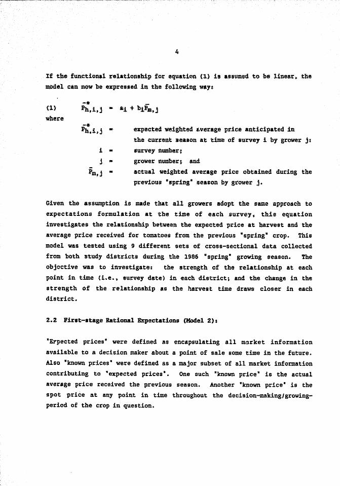
lithe functionalrelations~p for ~quatinn (1) isa.sumttd tobell.l1ear, the mQdel can now be expressed in the following .,.;

-ft _

(l)Ph,i,j .. &i+ bi,Pm,j

whe~e

i ..

j -Pm,j ..

expected _ighted .. ver.ge pric.e anticipated in

the current.eason at tilne of 8urv,e,. i bygrowe; j;

tn~rve,. tltmlb~~:

growetnumber. ;4nd

actual we~ghted averas., pr1ceobtaine4durlng the

previou, itspring· .ea8on by gtower j ..

Given the assumption io Jl1ade that all growers adopt thesam.e appro4ch to

expectations .f'otmulation atthetisne of each9urv~y; this equation

investigates the relationship between the eXll$cted p~iceat harvest and the

average price t.eceived for tomatoes from the previDus !tapring- crop. This

model was tested using 9 different seta of cross-sectional data. colleeted.

from both studydiatricts dur.ing the 1986 -opringit growing season. lhe

objcct!v.., was to investigate: the strengthcf the relationship at each

point in time (i.e., tJurvey date) in each distr.ict; and the change in the

strength of the relationship as the harvest time draws closer in each

district ..

2.2 Pir.t-stage Rational Expectations (MOdel 2):

"Erpected prices" wer.e defined 8S encapsulating all market information

available to a decision maker about a point of sale some time in the future~

Also "known prices" were defined as a major subset of all market information

contributing to "expected prices". One ouch Itknown price" is the actual

average price received the previous season. Another "known price" is the

spot price at any point in time throughout the decision-making/growing­

period of the crop in question.

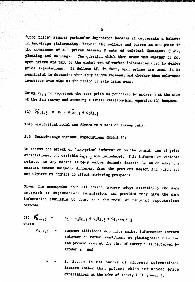
-,spot. Ptice- a.aumel 'p~t!cul.r imPQrtancf! becaus. it. ~ep,..e.ents •• halaut:e

inknQ'wl~dg. (infot;llllt1on) llet~enthe .,ellf!r. ;.ndbu1er •• toD.e poJ,nt in thflCQnt.iuuum.,()fall price, between. .2 seta of "Crltical deci.~Qn&(i •. i!! ••

·plantingal\d.eU.ill,> • the question whi.chtben ar.ole waawh.&tllero;,. not spot prices .te.p.rt of the global set l)fllllrlc.t lnfotillat';onused tp derl\"Q llrice expectation.. It iollowa '1f, in fact. spot prices 'are UIEld. It is ,JllE!anil1gfu1.tQdete~ne wh~n th~1 b~e~erelevant an4wnetner tl1atrelevance

inc%'ea.e$9~1: tixlle.. the period of'.al. 4rawsnear.

Using Pi • j to· ,;'epres.ent the spot price$$. p~r.cei vedbygrower jattbe'time

of the ith survey and a$swnins a linear relationship. eq~atlC)n (2) :becpme$:

(2)

'this statistical Illodel was fitted to 9 sets of survey dat:,a ..

2. •. 3 Second-stage Rational Expectations (Model 3):

'1/0 4ssess the affect of -non-price- information on the formul, ion Of price

expectations. the variable Zs,i.j was introduced. This information variable

relateo to any market (supply and/or demand) factors Zs which make the

current season uniquely diffe.rent from the previous season and which are

anticipated by farmers to affect marketing prospects.

Given the assumption that all tomato growers adopt essentially the sam.e

approach to expectations formulation. and provided they have the same

information available to them. then the model of rational expectations

becomes:

(3)

where

-it

Ph,i,j -

s •

curr.ent additional non-price market information factors

relevant tr market conditions at picking/sale time for

the present crop at the time of survey i as perceived by

grower j; and

1, 2, ••• n is the number of discrete informational

factors (other than prices) which influenced price

expectations at the time of survey i of grower j.

...•

6

·~~oQmOnZ.V'at~.ble8. (i. ell, i11fQrmation. ',indlcAtingeffects ,on $upply .nd

it1io~tion telatin..g :topotential delQnd) were lntli.ntained ~ll~.ch Burver .na t"Q.uB it. wa$;pos8ibletoe~~et1ie eh!D8es !n the 8~g¢ficanee ofth~$~ ·v.ti$ble8overt~~ .(i.'4 •• ftomplanUt\g. to l .. t~ !~ the piC:ldnsperiod)..

tlU.s, 'WOu,l,dnt)t.h&ve"eenposs~ble .iftheZavar.lablea luta.changed f~OO1cne

$ur:v~:r to: the nex t •

An e~pected p$:ice formulated in ,a past PE!tiodfor some time in the future

should encapsulate all of the ,information aVAilable and roc:ognisedat the

point $n time when that expectatidn was formulated. As such, the most

r'ecent past e)tp~ctedprice c:ould be viewed ., infot",Dlation in Ilddition to

last year\ price, current spot pticesand new nOn-price infof1'(JAtion. It

¥QuId include an element of the averAge price receIved in thesamese~son in

the pteviQus year but the size oftbiselementWQuld reduce a~ the current

season progresses. Thus • with the exception of possibly some mino.r double

counttng of th~ effects of the past season's average .price,the inclusion of

the most recently formulated expected price before the current one in the

model should exhaust all of the historical information available to and

observed by tbe grower.

The rational expectations model therefo.re becometH

- -- a1 + b1Pm,j +ciPitj + di.sZs,i,j + etPh,i-l,j where

-* Ph,i-lt j. expected weighted average price anticipated in the

cur.rent season at the timE: of survey i-1 by grower j.

-. Since Ph.i-l is a lagged variable from the previous period, it was not

po.ssible to estimatt:: this tnodel for the first field survey. This model was,

therefore, estimated only 8 times.

7

tle~lo:ve (19.56.) presented.hi8adaptive.expectations hypothe.ls .au

..... ach ,ear farmers rev!,. th~ price the1expectt()~preV'ail in the com11181,.r in.proportiQn' ,to the: e?:J:'OJ:they made 1npreditting

price this p~r1.(Jd.

*.. * Pt - Pt-l - B(Pt~l .... Pt-l) where

l. r

Later Nerlove (1.!lSS) restated his hypothesis in terms of the long run normal

price concept:

• __ • each period people revise their notion of I normal' price in

proportion to the difference between their current price and their

previous idea of normal price.

Using the same logic for the very short term it c.ould be stated that the

expect,ld priee at any point in the season could be perceived as the -normal­

price for that particular season and that growers may alter their notion of

the -no~l· price for that season in proportion to the difference between

the current spot price and their previous expectations for the season. That

is. spot price is perceived as encapsulating all of the relevant market

information about the ma1:ket at that point in time and growers may perceive

that information (i.e.. the spot price) as having an influence on future

prices. Thus the hypothesis could be restated for the present study as:

-* -* -* (5.1) (Ph,i,j - Ph,i-l,~' - b(Pi,j - Ph,i-l,j)

whfJre, as with N~rlove's hypothesi.s, O<b,l. That is. if b-l then the grower

would have no faith in his previous prediction and wo~ld adopt tbe current

spot price as his new expected price.

8

The .above equatiollCall be restated as:

The coefficients (i.e., ci and ei)were tested todetertnine whether they are

consistenttf.ith adaptive expectations for e$ch survey in each district.

This wa$ achieved by using the t-t.est of equality (homogenity) to teat

~ether ci • 1 - 91 for each s~rV9y(St(tel and 'lorrie, 1980).

z .. ~ x»ooled Data Models (MOdels 6 to 9)

In Models ~ to 5 it was assumed that on average all growers use the same

priceexpect&tion formulation process at each point in time. This

assumption coulr.l have been tested by estimating e.achmodel for each grower

using the 9 observations obtained from each grower over the season. The

coefficients of these equations -.rould then give an indlcation of the e~tent

of difference b~tweengrowers. However. owing to the small nu."!ber of

observations for each grower. this was not statistically feasible. It was

considered that it may still be useful to estimate the average effect of

such variables over the whole season. This was achieved by pooling cross­

$ectional and time-s~ries data.

These pooled data were used to test all of the previously specified models

except Modell (the cobweb model). The latter was not considered because, ~ -* -priori, it was expected that the relationship between Ph, i. j and Pm. j would

become less significant as the season progressed. Preliminary analysis

confirmed that this was the case. It seemed illogical therefore. to test

the explanatory power of this model relative to the whole season since this

would only servo to hide important changes in the pattern of relationships.

This would not necessarily be the case for the other models, since they are

more exptoratory and !. priori anticipations were not as strong ..

;42flumJ.ng lin(:lar relationships. the pooled d_t& V~r1.l1Qn6of Ho6el$ Z ,to '$ are as :follows:

~* -(1) lb.!. , j - a + bPm, j +cP i ,j + daZ,s, i • j

-* - -* (8) Ph.i~j .. a + bPm,j + c:Pi,j +ds'Zs,i,j + ePh.1-1,j and

-* -* (9) Ph.,i,j • a + CPi.j + el,)h.,i-l,j

where all variables are as defined earlier.

3. EKPIUCAL TESTING AND Ih~ERPiftAfIOH OF MODELS

The analysis of each model proceeded by determining whether any single one

of the coefficients and/or all of the coefficients combined were different

from zero at the .1, 1, 5, 10 B.nd 20 percent levels of eigni,ficance. The

adjusted coefficient of determination CR2) was used to i11dicate the

proportion of variation in the deperl.!pnt variables explained by the

independent variables.

Each model was checked for multicollinearity by eXamining the correlations

between independent variables and by calculating the tolerance of each

variable. The Durbin-Watson test was used to test for autocorrelation in

the pooled cross-sectional/time-series models.

Once the statistical acceptability of each model was established for all

surveys in each district, the acceptability of the models in terms of their

economic logic was examined. This was achieved by determining whether the

coefficients conform in relation to !.. priori expectations of sign and magnitude.

3.1 Cross-Sectional Models

The results for Models 1 to 5 using all available data are presented in Tables 1 to 5.

10

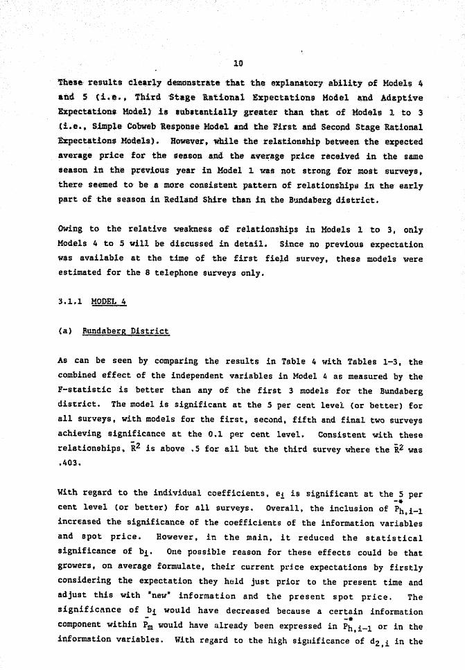
These re$ults c.l~.rly demonatrAte that the ~xpla~tor1 abJ,lity ()f }fQdel$ "4

abel S (.i.e.; 1hird. 'Stegellational Expectations Hod~l 4nd: Adaptive

~ectatipn8 ~dell i$ "Substantially ,great~r than that of Modele 1 to 3

(i.e., Simple Cobweb Response Model .nc:i the 'itst and Second Stage Rational txpectatioDS liodels)..lIowever,wb,ile th~ telationshlp between the expected

ave~age. pri.ce for tl1eseasor1 and the a:Y'er,ageprice rtceived in the ss,me

seaSon in. the pr~vious year in Kodel 1 waf! not strong for most survey.s,

there seEmled to be a more consi~tent pattern ofrelationshiptl in the early

part of the se~son in Redland Shire than !nthe Bundaberg d!strict •

. Owing to the relative 'Weakness of relationships in Models Ito 3, only

Models 4 to 5 will be discussed in detail. Since no previous expectation

Was available at the! time of the fi.rst fiel.d survey, the.s~Diodels 'Were

estimated for the 8 telephone surveys only.

3.~.1 MODEL 4

(a) Bundaberg District

As can be seen by comparing the results in Table 4 with Tables 1-3 t the

combined effect of the independent variables in !-fodel 4 as measured by tlle

F-statistic is better than any of the first 3 models for the Bl,lndaberg

district. The model is significant at the 5 per cent level (or better) for

all surveys, with models for the first. second. fifth and final two surveys

achieving significance at the 0,,1 per cent level. Consistent with these

relationships~ a2 is above .5 for all but the third survey where the i2 was

.. 40.3.

With regard to the individual coefficients, e1 is significant at the 5 per -* cent level (or better) for all surveys. Overall, the inclusion of Ph

9i-l

incr~ased the significance of the coefficients of the information variables

and spot price. However t in the main, it reduced the statistical

significance of bi. One possible reason for these effects could be that

·growers, on average formulate, their current price expectations by first.ly

considering the expectation they held just prior to the present time and

adjust this with wnew• information and the present spot price. The

significance of bi would have decreased because a certain information - -* component within Pm would have already been expressed in Ph,i-l or in the

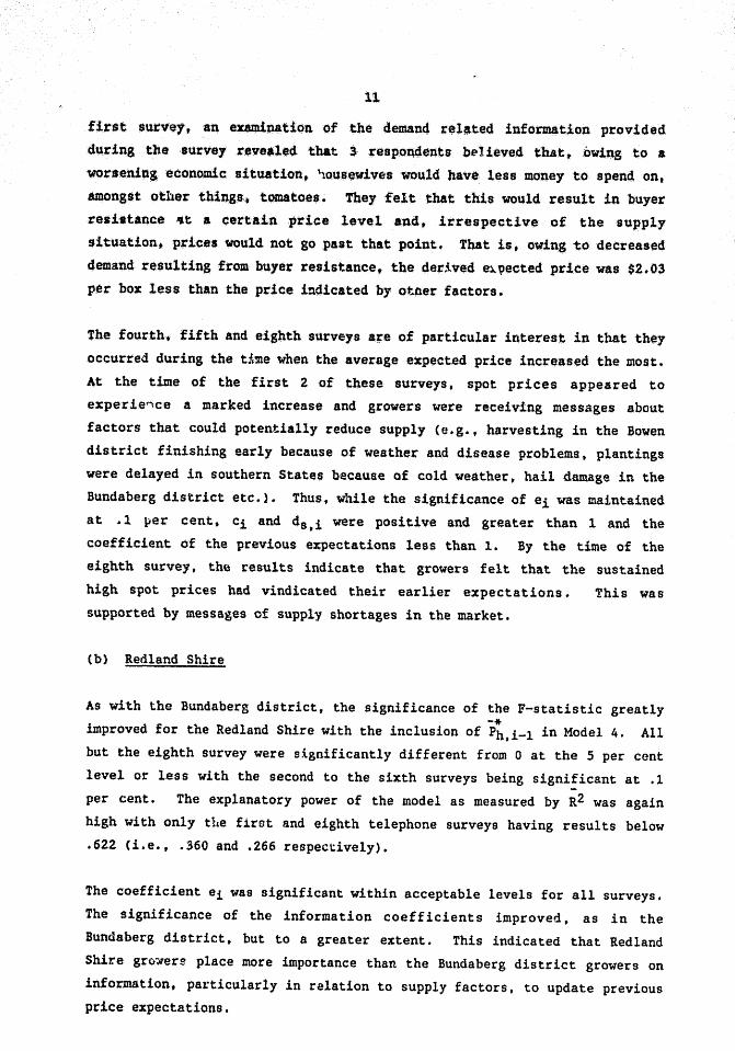
information variables. With regard to the high significance of d2,i in the

11

f!r$t survey tan examination of the dentan4rA;!1~ted informa.tion provided

.duringthe 'flurvay reve.ledthat 3 respondents 1) pI ieved tha.t ~ owing to a

wor.enil1g econcnnic situation. ~ous~v~s would have less money to spend on,

&nongst other things" 'tomatoes. They felt that this would result in buyer

resiat.nce "'ta certain price level all.d, irrespective of the supply

$~tuation .. prices would not go past that point. Tbatis, owing to decreased

demand re$ulting from buyer resistance, the der.ived e1.gected pric$ was $2.03

p~r box less than the price indicated by otfter factors.

The fourth. fifth and eighth surveys are of particular interest. in that they

occurred during the ti.ne when the average expect.ed price increased the most.

At the time of the first 2 of these surveys. spot prices appeared to

experie'tce a marked increase and growers were receiving me.ssages about

factors that could potentially reduce supply (e.g., harvesting in the Bowen

district finishing early because of weather and disease problems. plantings

were delayed in southern States because of cold weather. hail damage in the

Bundaberg district etc.). Thus. while the significance of ei was maintained

at .1 lIer cent, ci and ds,i were positive and greater than 1 and the

coefficient cf the previous expectations less than 1. By the time of the

eighth survey. the results indicate that growers felt that the sustained

high spot prices had vindicated their earlier expectations"

supported by messages of supply shortages in the market.

(b) Redland Shire

This was

As with the Bundaberg district, the significance of the F-statistic greatly -* improved for the Redland Shire with the inclusion of Ph.i-l in Model 4. All

but the eighth survey were significantly different from 0 at the 5 per cent

level or less with the second to the sixth surveys being significant at .1

per cent. The explanatory power of the model as measured by R2 was again

high with only the first and eighth telephone surveys having results below

.622 (i.e., .360 and .266 respectively).

The coefficient 8i was significant within acceptable levels for all surveys.

The significance of the information coefficients improved, as in the

Bundaberg district, but to a greater extent. This indicated that Redland

Shire grG7erS place more importance than the Bundaberg district growers on

information. particularly in relation to supply factors. to update previous

price expectations.

12

-* The effects of the inclusion of Ph.i-l on the -known- price coefficients

varied slishtly. In the main. the significance cf bi decreased while two

coefficie1'.ts became significant at the 5 and 20 per cent levels.

The reasons for the above observed changes are broadly similar to those

given for the Bundaberg district.

The resulte for the fifth, seventh and eighth surve,'s are of part.icular

interest due to the large increase in average price expectations nt those

times. The relatively large and positive value of dl,! in the fifth survey

(i .. e., 2:.112:) was probably caused by reports of hail and other weather

damage to crops in the Bundaberg district and the early cessation of picking

in Bowen affected price expectations at that time. While previously held

price expectations influenced the for,mulation process, the magnitude of ei

(i.e.; .697) indicates that only part of these past expectations was

relevant (i. e.. some of the information content of the previous price

expectation was superseded by the current supply situation). In the seventh

survey the magnitude And sign of the coefficients of significant variables

(i.e. t d1,i and ei) clearly demonstrates the importance growers placed on

both the new knowledge that a supply shortage was likely and previously held

expectations. That is, it is estimated that the Redland ~istrict growers

adjusted their previous average expected price upwards by approximately

$2.00 a box because of the new supply side information they had received.

The result for the eighth survey is puzzling in that the large and

marginally acceptable ail together with the signific~nt ei (i.e •• at the 1

per cent level), would normally indicate that the avr~age price expectations -* are largely explained by Ph,i-l and the other variables not covered by the

model. However, 15 out of the 19 growers responding to this survey in this

district recorded a shortage of supply message and all but one increased

their price expectations. Also. spot prices were unusually high at that

time. Thus. it would be logical to anticipate that both ci and dl.i would

be highly significantly positive and large in magnitude. A possible

explanation of this apparent anomaly could be that the recorded values of -* Ph,i were regressed against 1S values of 1 ::or I-he supply information

variable and 12 values of $26.00 for the spot price variable. Thus while

most growers agreed that the shortage of supply and spot prices would

increase average expectations. these relationships would have been obscured

because of the common values given to both variables (i.e., graphically.

13

moatobservatlaru, wpuld f.ll ona line parallel to the Y-axl.s from a common

point on the X-ana). this interpretation is supported. by the poorove;:all

fit of the equation for the eighth ,survey.

i

The fourth telephone survey it also of interest because of the highly

significant but negative and relatively large values for dl,!. This wac

mainly due tQthe e~pectation of no null large supplies of t.omatoesfrom the

Bundabflrc district and the good weather conditions prevailing at the time in

both ~he Bundaberg district and Redland Shire (i.e., both these factors

reduced .veraged price expecta.tions).

(c) The Two Districts Ccmpared (Model 4)

-* The addition of Ph,i-l in Model 4 greatly improved the explanatory power, as

measured by i 2 t in all surveys in both study districts.. The F-statistic

became significantly different from 0 at acceptable levels for all but the

eighth Redland Shire survey, which as discussed above had data problems.

The significance levels of the lIadditional· information variables were

either naintained or improved compared with Model 3. "Additional­

information affected average price expectations more in Redland Shire than

in the Bundaberg district. For example, d1,i is significant at acceptable

levels in 6 out of the 8 surveys in Redland Shire compared with 4 in the

Bundaberg district. Also, this coefficient is larger in magnitude in the

former district in (; 'of the surveys. The coefficient ei is highly

significant in all surveys in both districts ~ However. it is larger in

magnitude in 5 surveys in the Bundaberg district. thus indi~ating s greater

hesitancy in that district to change expectations from one point in time to

the next.

3.1.2 MODEL 5

(a) Bundaberg District

The results for. Model 5 (adaptive expectations) for this district and for

Redland Shire are presented in Table 5. In addition to the size and levels

of $ignificance of the coefficients, the F-statistic and Rt, this table also

provides the values of the t-statistics used to test whether, on the basis

of the data available, the coefficient ci is or is not significantly

different from 1-ei for each survey.

14

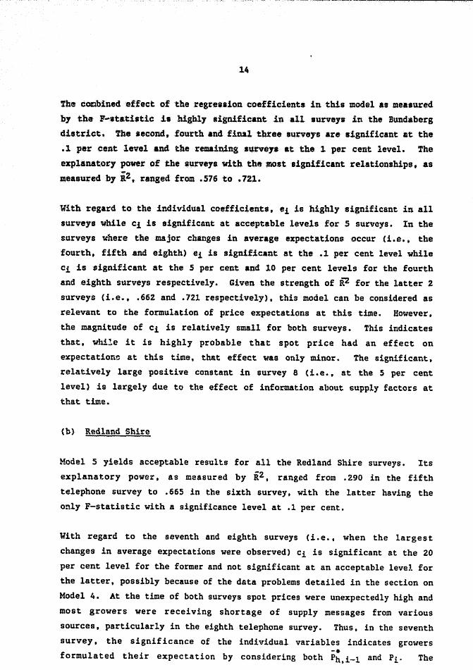
The coznbinedeffect of the ,regression coefficients in this model atsQ1easured

by the P-st&ti.tic:: is ,highly lignificantin all survey • .in the Bund.berg

dia.trict.The .econd,fourth and final tbreeaurveys are significant at the

.1 par cent level an4the ~emaining survey. at the 1 p(!r cent level. The

explanatory power of the surveys. ~tb the~$tsignificant re14tionships. a. me.suredby i 2, ranged from .576 to .721.

Vithregard to the individual coefficient., 8i is highly significant in all

surve,s while ci is significant at acceptable levels for 5 survoys. In the

surveys where the major changes in average expectations occur (i.e. , the

fourth, fifth and eighth) ei is significant at the .1 per cent level while

ci is significant at the 5 per cent and 10 per cent levels for the fourth

and .eighth surveys respectively. Given the strength of i2 for the latter 2

surveys (i.e .. , .662 and .. 721 respectively). thls model can be considered as

relevant to the for.mulation of price expectations at this time. However.

the magnitude of ci is relatively small for both surveys. This indicates

that. whi:!.e it is highly probable tbat spot price had an effect on

expectations at this time, that effect was only minor., The significant.

relatively large positive constant in survey 8 (i.e .. t at the 5 per cent

level) is largely due to the effect of information about supply factors at

that time ..

(b) Redland Shire

Model 5 yields acceptable results for all the Redland Shire surveys. Its

explanatory power, as measured by i2. ranged from .290 in the fifth

telephone survey to .665 in the sixth survey. with the latter having the

only F-statistic with a significance level at .1 per cent.

With regard to the seventh and eighth surveys (i.e., when the largest

changes in average expectations were observed) ci is significant at the 20

per cent level for the former and not significant at an acceptable level for

the latter. possibly because of the data problems detailed in the section on

Model 4. At the time of both surveys spot prices were unexpectedly high and

most growers were receiving shortage of supply messages from various

sources, particularly in the eighth telephone survey. Thus, in the seventh

survey, the significance of the individual variables indicates growers -. formula ted their expectation by considering both Ph. i-1 and Pi' The

- - - -lS

magnitude of ci was relatively small (i.e., not approaclling 1) beCal.1Se

picking had commenced 2 to 3 weeks beforehand and the prices received tben

would reduce the overall average for the season below the C"7.1rrent spot

price. In the eighth survey, the constant is large and significant because

of the effect of variable& not covered in this model.

(c) The Two Districts Compared (Model 5)

Generally the V-statistic for each of the surveys i~ signifieant at lower

levels in Redland Shire than in the Bundaberg district. The explanatory

power of the model, as measured by i 2 , is also much less. with Redland Shire

having only 1 survey with i2 above .6 compared with 4 in the Bundaberg

district. The significance of the 81 coefficients are not as tight. in

Redland Shire as in the Bundaberg district but they are still all

significant at levels between the .1 per cent .and 10 per cent levels. The

magnitude of tbis coefficient is larger in the Bundaberg district in 6 out

of the 8 surveys. Five out of the 8 ci coefficients in the Bundaberg

district are significant at Acceptable levels compared with 4 in Redla.nd

Shire. With the exception of tbe fifth Redland Shire survey the magnitude

of this coefficient is less than .5 for all those with &cceptable levels of

$ignificance, thus indicating that, in general, the .probable effect of spot

prices on average expectations is not great in both diRtricts.

In summary, it would appear that. while Model 5 is relevant to both

districts, it is more effective an a model of price expectations in the

Bundaberg district than in Redland Shire.

(d) Model 5 and the Adaptive Expectations Hypothesis

As explained earlier. the t-te$t for equality was applied to determine

whether. on the basis of the data available, ci is or is not significantly

different from l-ei for each survey. If these two values are not

significantly different from eAch other, the data are consistent with the

adaptive expectations hypothesis. That is, the data suggests there is no

reason to reject the hypothesis that tomato growers revise their average

expected price for the season in proportion to the difference between the

current spot price and their previous expectation for the season.

-

,- · RIi* .... cw ,.- ,. m._

16

TbJ,ste.t. rev.aledtb.f,tt.hemQdel i •• Inde,d. ·::!t)n.il-t~twith .daptive

expectatioIlI foralt a tel,phone lIu~e,..forth&Bundaberg diat!:lct at the 5 and lQ p'er ceIlt.i$~fica~celevel. and fot all but thetbJ,rd and eigb.th

telepholleaurveysfot'1le41andSlU.rs. 'nl,u •• it co"ld be said that, with only

min()t' exceptions, t--.togrowers in both district. used the amrket .signals

as relA1(td througn theapotprice toadjuat their average -expectation. frQm

one period. to the next during the season. In the! $utv',I,where the.

results .re 'not consistent witb adaptive expect.tiona, thecoQst.nts are

significantly different from zero at the Sper cent level and they are

relatively large ana positive. This ,1ndicate$that iJnportant explanatory

variables 81".e 1!xcluded from th. model in tnele cases (e.g. II information

about SUPP"',1 f&~tora).. AI_o, .as alreadyment.toned .ev~ral t;l.mes, with

regard to the eighth survey, the. r~petition of the .ante value of Pi would

have ~dver£ely affected the ability of the tegtes.ion analy.sis to estimate -0-

the relationship between that var!.bl~ and lil,i. Tbe t-statistics of

equality for all sur~eys are presented in Table S.

3.2 Pooled Crocs-sectional/tfae-Ieries HDdels

'the results for the pooled cross-sectional models are given in Table 6. The

Fir$t and Second Stage Rational Expectations Models (i.e., Models 6 and 7)

appeared to produce promiaing results but the Durbin-Watson test suggested

the presence of serial correlation in both models in both districts.

The Third Stage Rational Expectations Model and the Adaptive Expectations

Model (i.e., Models 8 and 9) became even more powerful when the data was

pooled. In the former the coafficients for spot prices. information about

factors relating to supply and the expected price formulated in the mos.t

recent period bafore the current period, were all significant at the .1 per

cent level for both districts. The coefficient for information about

factors &:elating to demand was significant at 1 per cent for the Bundaberg

district.. 'these results clearly indicate that growers, on average, use

these variables throughout the $eason to formulate average price

expectations for the season. The coefficients of all the variables in the

Adaptive Expectations Model (1 e., Model 9) were significant at the .1 per

cent level, also indicating a close fit for this model throughout the

s~ason. This model was also shown to be consistent with the adaptive

expectations hypothesis.

•

,aaa pa ,

17

%omat;Q 'Stowers. 11k- l1\O*thorticultttralprodtu:etfJ, ,eQ and de. .1 tet:botlttha

lev,l :.nd th- timinsof tb.eit Pl:'Q~~c;t1()nduri~g aSt'owing'season. these

witblJ1 •••• ct;l.'.uppl,.~ejpon.ee~.llnot be capt,uredby the traditional

&8gt'~g.ti:'1e a.nnual tim.-,erie.allpro.ch.

'lh$ p;-lncipal .im of thispapttr u_ tb"deV'elop anaeva'1Qat. a se.rles ()f

models detigned to qgantify thepr1<:e. ,t!txpectatlonfo~lat:l.on behaviour of

tomato grQw\!!ra and to investiga.t.e bowtht!8$pr!ce ta:ttpectations changecl

withinonegt'ow1ugseason.

Overall, the result. are consistent 'With economic rationality andsugge$t

that growers attribute considerable importance to being able to formulate

realistic prtce expectations. A. one WQuldel(pect. the eviden<:e is that

grower,a· expectations ate very mucb influenced by their previously held

expectations. In this r.egard. contrary to what one may think9 the growers

in the new and expanding tomato growing area (Bundaberg) appear more

J;'eluctant to change their expectations over time than the growers in the

more traditional di~trict (Redland Bay). The adaptive expectation

hypothe$is is supported by the analysis' which mt!anB that when tomato growers

do alter their price expectations, they d'O so largely in response to changes

in the spot price. This finding emphasises the importance growers place on

the need for an accurate (and trusted) market reporting service.

.. # . .i .. 18

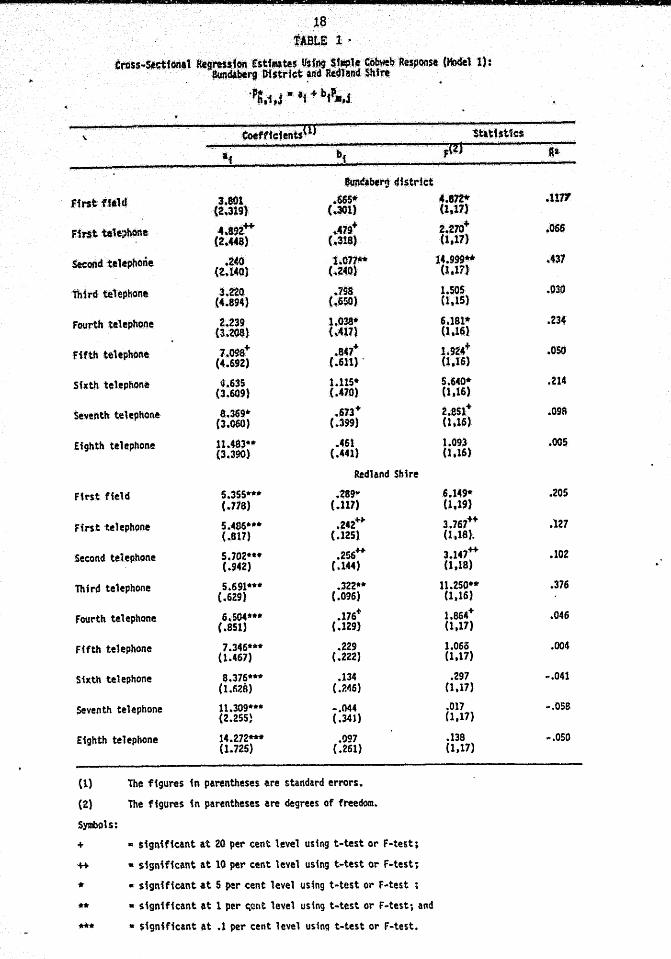
fABLE 1 •

tro$s"SJ~iOrt.l~greSl1~£stf.te$. tf${Jjg$f".l •. ~~. 'Re.PQnse(Hodel 1): , . . '1km~~ Pbttt~t~nd ,Re.dhnd $hi"

'P;.f;S- !Ii +bf~.,J.

\.

. "w .,,'"

~abt~ dt$trict

ffrst·ft.'d .3.801 _$6S· 4.872* .. 1171 (2.319) (~~1) (1,171

f1r$ttele~hone 4.a~!++ (2.448)

.. 4.2!l (.318)

t.270+ (1,11)

.066

SeeOj'idtelephone .2CO t.0711o'* 14.999" .437 (2..140) (-02(0) Uti?}

lhh'd telepliQne 3.220. .198 l4.894) ,.~~).

1.505 (1.15)

.030

FOUrth teleph~ne 2.239 1.038· 6.181-- .234 (3..:2Q8) (~411l (I ,un

fUthte1ephf.)ne 7.OSS+ .841+ 1.924+ .050 (4.692) (.611) . (1,16)

Sixth telephone 4.635 I .. US* 5.640* .214 (3.609) (.,410) (lt16)

Seventh telephone 8~3G9* .673+ 2.851:+ .098 (3.0Q0) (.399) (1,16)

Eighth telephone 11.483*· ,.461 1.093 .00$ (3 .. 390) (.441) (1.16)

~dland Shire

Ftrst field 5.355-·· .289" .6.149- .205 ( .. 718) {.U7) (1119)

Fi.rsttl!lepb()ne 5.466·" .242+" 3..761++ .127 ( .. 817) (.12S) (1 tI8)~

Second telephone 5,102 .... .256++ ~.141++ .10Z (.942) (,.144) (1.18)

Third te1ephQne 5.691··· .322·· 1l~250u .376 (.629) (.096) (1,16)

fourth telephone 6 .. 504 .... .176+ 1.664+ .046 C .851) (.129) U,11)

Fifth telephOne 7.346· ... .229 1.060 .004 (1.467) (.222) U,11)

Sixth telephone 8.316· ..... .134 .297 ... 041 (1.628) (.246) (1.11)

Seventh telephone 11.309**- -.044 .017 ... 058 (2.255} ( .34l) (1,17)

Eighth telephone 14.212 ...... .097 .138 ... 050 (1.725) (.261) (1,11)

(l) The figures in parentheses are standard errors.

{al The figures in parentheses are degrees of freedom.

Symbols:

+ • significant at 20 per cent level using t .. test or F-test;

++ • significant at 10 per cent level using t-test or f-test;

'1ft • significant at 5 per cent level using t .. test or f .. test ;

'il''' • $ign1ficant at 1 per ~Cflt level using t-test .or f.-test; and ... • ~i9nlficant at .1 per eent level usin!l t-test or , .. test •

L. 19

TAB.LE2

CtoS$.Se~t{~"'l :~gre~don' ~E$d .. ~s Y$11)9, Ffl'$ts~.ge btt<mal £~Pfletltf9~$ (~1~h8~~r, N$tdct Jm!b.f\la.n~Shtre ~

',".l',~ -Ii +'bl~ .. ~J *.~iPU . ", • ,

$liMY ~oeftfei'n," t, .,bf ~1

Qu~~rgtn$tri,ct:

f1~tffeld.' 5.971+ {-121i ,,",ii,135'

(3.156) .320 (,,~l 2.531+ .145 "(~t16)

FfrsttelephQn, 2.67% ,496+ .313) (~~~12) (.:319) (·.nl

1.;606 .OG3 (2,I6)~

$tcqnd 'te1~phone ... 604 .940* ~lao, (2.445) '(,,321) (.2()S}

7.4~ .. 4$2 (2.l51

Third' ulephon~, 21'294 .555 .231 (5~238) ( .110) (~3$7)

.898 -~Oll (2~14)

f'Of,lr.;h, telephone 1 .. 552 .481 .3$7++ (3~0221 (.S23) (.204)

S.884~ .319 • (~,14)

Fifth tel~phont 4.624 .72,6 .. 119 (6 .. 412) (.G59). ( .. 315)

1.083 .. 010 (~.lS)

S1)(th~ehphon. -~a49 .838+· .5.16-(4.053) (.438) (.231)

6.029* .312 (2.1S)

Seventh telephone 6 .. 570" .447 .248 (3 .. 435) (.444) (.221)

2.018+ .113 (2.15)

Eighth telephone 9.014++ .281 .138 (4.524) ( .505) (.162)

.876 -.016 (2,14)

Rediand Shi re

First field 4.346·" .321-· .090 (.964) • (.10S) (.110)

5.842~ .338 (2.17)

first t~lephone 3.380+ .200+ .463 (2.028) ( .129) ( .409}

2.555 .141 (2.,17)

Second telephone 1.100 .330· • 38S"" (2.226) (.139) (.191)

3.732· .223 (2.17)

Third ':.elephone 4.154·* .241' .130 (1.287) ( .110) (.121)

4.147- .296 (2.13)

Fourth telephone 4.486- .• 045 .266+ (1.910) (.123) (.153)

1.551 .064 (2.14)

fifth telephone 1.168 .213 .337++ (3.036) (.2(14) (.165)

2.734++ .162 (2.16)

Sixth telephone 6.163 .131 .144 (4.825) ( .252) (.294)

.261 -.089 (2.16)

Seventh telephone 6.728+ -.149 .416+ (3.930) ( .340) (.296)

.995 ... 001 (2.16)

Eighth telephone 11.029++ .061 .132 (5.361) (.272) (.200)

.272 -.088 (2,16)

(1) The figul"e$ in parentheses are standard errors.

(2) The ffguru in parenthesis are degrees of freedom.

Symols:

+ • significant. At 2Q per cent level u~in9 t-tcst or F-test. . , .# • d~tftcant It. 10 per cent level USing t-test or F-test;

'It 1$ stgntftcant &t 5 per cent level us1ng t .. test ~r F-test;

• significant at 1 per cent level using t .. test or f-tellt; and

• significant It .1 per cent level using t-test or F-test.

,.,

'?:O'

tA$Le·3 Cron~~c~1o\'JI1 ~,"-,$$ib!ltst1.te$ Usfli9Secend~, ;$U~Rat1Mal~p~~tat1c:m$ ,(Hot!et3h lSlindlb6rti nfs~rtct, .~ntfRed .• 'vlSMre

~.i.~ '. If + ftl •• J t CtPi.J + di. i Zr •. ltJ + ~ •. ii'Z;f • .f

CoeftfcientsnJ. .ot

~t.ttstic;s \$U~

411 ~.i ft2l ftt " at ,lit c. ... . &mdabettt di$trfct

FfrSt ffeld 4.895 .156++ •• !5$ .. 014- .. 225 1.143 .031 (.4.041) (.358) (.249) ll,,4~) (.682) (4,.14)

fir$t telephone 31t133 .110* -.091 .l~S2 -2.030++ 1.99~+ .1$2 (3.032) (.321) (.3l0) (.71$) (.978) (4,14)

Second telephon6 ~ .• 50S .ssa· .209 .. 636 S.406w .43; (2.435) (.328) (.206) (. .. 593) (3,14)

Third telephona 1.842 .643 .188 .902 .• 814 ... 03G (5.326) ( .. 785) (.394) (1.088) (3.13)

fourth telephone 2.132 .l81 .360++ 1.005 4.611* .408 (2.985) (.515) ( .200) (.176) (:?~13)

Fifth telephone 3.927 ,820 .139 1.105 •• 948 -.009 (6.585) ( .674) (.3l1) (1.304) (3,14)

Sixth telephone .SGg .814+ .442+ -1.01S -1.2.43 3.887* .. 405 (4.107) (.470) (.234) (.876) (.983) :4,13)

Seventh telephone 6.550+ .3M .292 ... 310 1.353 .059 (3.538) (.482) ( .256) (.883) (3.14)

Eighth telephone 5 .. 501 .~5l .247''' 1.493+- 1.456 .079 (4.860) ( .481) C .170) (.956) (3.13)

Re4land Shire

First field 3.141** .314" .107 .506 .522 3.112- .368 (1,.008) ( .. Ill) ( .. 109) ( .. 49l) ( .491) (4~15)

First telephone 3.298+ .203+ .411 .143 1.631 .091 (2.111) ( .. 134) ( .422) (.S66) (3*16)

Second telephone -.251 .458·· .416- .980++ 4.446· .352 (2.236) (.141) ( .18S) (.468) (3.I6)

Third telephone S~070" .,55· .088 .Z45 2.701++ .255 (1.450) ( .111) (.148) (.459) (3,12)

Fourth telephone 5.377* .102 .162 -.784 1.478 .082 (2.10S) (.132) (.177) (.695) (3.13)

Fifth telephone 4.142+ .325++ .103 2.02** 7.536** .521 (2.386) ( .157) ( .140) (.562) (3.15)

SiXth telephone 2.494 .228 .295 '.664* 1.795+ .117 (4.659) (.231) ( .214) ( .7.64) (3,15)

Seventh telephone 6.224+ ... 024 .308 1.508 .726 .934 ~.OlS (3.988) (.357) ( .3lS) (1.239) (2.414) (4,14)

Eighth telephone 11.602++ .O~6 .120 -.350 .206 -.152 . (5.792) ( .280) ( .216) (1.076) (3.15)

(1) The figures tn parentheses are standard errors.

(2) The figures in parentheses are degrees of freedom.

Symbols: I

+ • significant at 20 per cent level using t .. test or ,-test; .

++ • significant at 10 per cent level using t .. test or F-test;

'* =- significant at 5 per cent leve~ using t-test 01" f·test; .. • significant at 1 per cent level usfng t-test or F-test; and ... ,.. • $ignificant at .1 per cent level using t .. test or F-test

21 ... -TAl:JtP i

ero$$":~t.1.Ohll ~e,sf~· t$~t.te, .lhfnj.T6ird .Stlge R#tionll ~~«;tat1~$ .( .. I '4); RuA~bt~tlfs~tfc~ .l'Id }tedllnrl SIli ...

~.i)~ ~:·t +btP •• J +CtFtf).1+dl.tt~,f.J.'" 4~J~~.t.~ ;. et~Jf;'lJj .. . . ... \'tj"'.1-"~~ •

0'

I « COetffcfefltst1) S~tbtic:s

~t b. cf 41•t <12•1 &i F(aJ Itt

8un~~rq dfstrtct Ift"$~.~lephQft. t~8$O .208 .. .. 259 ~7U+ ... 2i.t42~ .715*** t •. 226*** ,696

U~888) (~~al) (.2<8) ( .. 475) (.G14) (.l56) (5.13)

SecQ(1<1telephon~ .. 4·.401- .528* .. 231+ ..... 089 .1%3"'* 13.'l53H'* .74.1 U.898) (.23tH (~140) (.4Sg) (.18l) (4.13) .

i .. 251** Third telephone Z~416 ... 311 ... 142 ~94l 3.703· ..403 (4 .. 046) C~6(4) (.316) (.826) ( .• '387) (4,12)

Fou.fth telephone 1.245 - .. 109 .. 55Ztt 1.023++ .31S*** 9~a65** ~i'Q3 (2.450) ( ~36S)· (.120' (.4.97) '( .J3S) (4.11)

Fifth telephone .. 3.440 -~035 .267+ 1.ap~ ~$90"** 10. 235*-H' .. 684 (3.905) (.406) ( .181) (.142) (.158) (4,13)

S;~th telephone .. 183 .580+ .254 - .. 69'3 .. 1.280+ .406'" 5.988** .595 (3,;398) (.403) .206 ( .1lZ) ( .811) (.152) (S.12)

Seventh telephone 3 .• 243+ ... 31:1- .231+ ... 205 .1"~"'** 12'.154* .... .124 (1,,996) (.267) ( .1391 ( .481) ( .119) (4,13)

Eighth telephone 3.523 -.074 -.080 .831+ 1.0'26*'" 11.s..4*** .. 725 (2.619) ( .269) (.109) (.536) .183 (4.12)

Redhnd Sh f re

First telephone .611 .051 .378 .400 .563· 3.672* .360 (Z.016) (.124) (.356) (.434) (.202) (4.15)

Second telephone -2.316 .26S· .347* .866· .642·· 8.821**· .622 (1.805) (.121) 0 (.146) (.359) (.162) (4 .. 15)

Thi rd telephone 3.S2a*~ .146* -.134+ .843*· .628·"* 14.301·" .780 ( .831) ( .(66) ( .Ogo) (.213) (.115) {4.1l}

Fourth tele;'lhoM 1.850+ ... 134+ -.125 -1.658** 1.On·" 14.167 ..... .178 (1.192) ( .015) (.116) (.419) ( .117) (4,H)

Fifth telephone .104 .209+ .069 2.112*'" .697* 10.699*** .€S3 (2.318) (.134) ( .115) {.458} (.237) (4.14)

Sixth telephone .. 5.483++ -.014 .440· .910" .860*"· 12.60~'** .721 (2.962) ( .131) (.156) ( .446) ( .149) (4,14)

Seventh telephone .. 1.316 -.093 .156 2.06511 -.415 1.036"· 7.512'** .644 (2.774) (.2IZ) (.189) (.142) (1.447) ( .200) (5.13)

Eighth telephone 7.417'·' .120 -.008 .924 .555** 2.633 .266 (4.810) ( .224) ( .177) ( .952) (.180) (4,14)

(1) The figures in parentheses are standard errors

(2) The figures in plrentheses are degrees of freedom

Symbols:

+ • significant at 20 per cent level using t-test or F-testj

++ .. signfficant at 10 per cent level using t-test or F-test;

" • significant at 5 per cent level using t-test or F-test ;

--. • Significant at 1 per cent level using t-test or f-test; and

11 .. • significant at .1 per cent lev~t using t-test or F-test.

22

TABLE 5 ... CrOsll·Se~tlOl1'l, ~"s$1<mEiti.~$ l;sJns Aa.pti~. E,;peetlt1t\ns

• l~1...shBIitlrl~berg Jhstrfct Me! Rec!lantt'Shint

'h.1:S .. l i·+ C1Pf.J ... etPh.t-l,j

. Statistics

f(2)

~ber~ ~istrtet

flrsttelephone 1;1S4a 1 ... .31 .62~ 6:341**' ~360 -.6368 (Z.165) (2.345) (.181) (2.17)

Second telephone -3.021+ ~374~ .894"*· 21.314**-- .693 1.2802 (1.849) (.1lO) (.163) (2.16)

Third ~elephone .811 .. ~082 1.118-- 7.015** .414 .0834 (2.961) (.276) (.333} (t.1S)

Fourth telephone .953 .320· .543*11'* 16.699*" .662 -.7850 (i.111) (.125) C.1Zi) (2,14)

Fifth tel.tphone .011 .213 .785"-* 9.920'" .498 -.0091 (4.548) ( .209) ( .ISl) (2.16)

Sixth telephone .005 .431H •. 5)2" 13.249*'" .576 -.2:273 (2.BS2) ( ."213) ( .154) (2,16)

Seventh telephone 2.143 .274*'1: .. 565"· 22.756*** .107 -1.2394 (1.859) ( .094) {.O90} (2,16)

Eighth telephone 4.471* -.U9++ 1.024*-- 22.968·" .721 .5804 (2.096) ( .062) ( .152) (2.15)

Redland Shire

First telf!pnone .891 .396 .571** 1.313'" .401 -.0871 (1.889) (.335) ( .113) (2.17)

Second telephone -.027 .197 .789**· 10.540·* .Srl -.0571 (1.826j (.153) (.lSS) (2.17)

Third t~lephone 2.988· .OM .560" 11.591'** .585 -2.2617 (1.122) . (.095) (.135) (2,l3)

Fourth telephane .894 .239++ .525- 7.0U** .445 -.1764 (l.S4!;;) {.129} { .203} (2,13)

fifth telephone -1.161 .687++ .311++ 4.S6S· .290 .0103 (.3.474) (.336) (.152) {2,16}

Sixth telephone -4.541+ .364* .921*·· 18.857*** .665 1.2660 {l.169) (.167) (.ISl) (2,l6}

Seventh t~lt~h~n~ .. 1.131 .1.80+ .933**« 9.941'" .498 .6899 l!.ll1) (.206) ( .231) (2,16)

Eighth tEll,C!~fia £} '.'71* .005 .471** 4.877* .301 -2.2764 i,~.302) ( .l68) ( .151) (2.16)

(1) The figures in parentheses ire standard errors. (2) The figures in PAl'entheses are degrees of freedOll. Symbols:

+ • sIgnificant at 20 per cent level using t-test or F-test.; . ++ • Significant It 10 per cent level using t-test or F-test; .

* • significant at 5 per t"nt level ustng t-test or F-test; . --. • significant at 1 per cent level using t-test or F-testi and

*** • Significant at .1 per cent level using t-test or F-test.

23'

TAaLE 6

PooltdcroSS"Sectiona.'lITi.Sflrtes Resre. nion. En tmates (MOdels 6 to 9). 8undiberg District lnd'~~41and Sltfr-e

\ Coeftfcfents(l) Shtbtics District

Bundabero

Redland Shire

Bundaberg

Redland Shi r~

iI b

P*h.i.j·· 1+ bP,.. + CPf,j'

2.414++ .SOO·* .347·" (1.418) (.le3) .( .029)

3.582*"· •. 129+ .358." (.609) (.083) ( *021)

2.695'*+ .478" (1.403) (.179)

.330*·* .576++ {.029} (.344)

-1.450** (.530)

3.152'.. .157* .340·" 1.046·*· .572 (.593) (.080) (.021) (.265) (.641)

. lit FtZ)

Model 6

80,.591"· (2,155)

142.8S5**" (2.1~6)

Modt!l 7

44.235*"* (4,153)

8a.145 ...... (4,1641

~·b.itj· a + b~m + CP"j + d1l 1,i.j of d22z.i.J + eP\.i-l.J J40del 8

Bundaberg .930 .094 .173'" .857'" -1.747** (l.061) ( .14I} ( ~O241 (_253) (.S07)

Redland Shire ... 594 .014 ~173·'· Lag1 .... .711 (.537) (.061) (.020) ( .Z09) (1.161) .

P*h.f.j • a + cP i •j + eP*h,i-l.J

Bundaberg 1.731** .20764 1)

(.511) (.025)

Redland Shire ... 512 ,209"· (.484) ( .021)

tll The figures in parenth~5es are standard errors.

(ll The figures in parentheses are degrees of freedom

.656**" 95.079**' . (.054) (5.132)

.837·" 151.594*** (.OSS) (5.142)

foIodel 9

.635**~ .206.359'*· , (.05l) : (2,143)

.841***' 296.292*** , (.071) . (2.145)

Rl Durb1"r3) Watson

.S03 1.113

.628 1.169

.524 1.126

~661 1,321

.774 2.267

.842 1.968

• .'39 2.166

.801 t.918

(3) H (i.e.. sample size) for this statistic is the sum of ~he degrees of freedom for F plus 1

Symbols:

• significant at 20 per cent le~el using t-test or f-test; .

++ • significant at 10 per cent level using t-test or F-test; .

* • significant at 5 per cent level using t-test or F .. test; .

• Significant at 1 per ceht level using t-test. or F-test; and . ",. • significant at .01 per cent level using t·test or F-test •

24

NERLOVE. M. (1956). -Estimates of the Elasticities of Supply .of Selected

Agricultural Commodities-, 30urnal of Farm Economics 38.

NElUaOVE. M. (1985) ,The Drnamics of Supply;: Estimation of Farmers' Response

to Price. John Hopkins Pte$s, Baltimore.

STEEL. R.G.D. and TOXRIE~ J .H" (1980) ~ Principles and Procedures of

Statistics A Diametrical Approach, McGraw-Hill, Sydney.

WHYBROW. E. (1987), Price Expectation Formulation and Information Sources in

the Queensland Tomato Growing Industry, Unpublished Master of

Agricultural Science Thesis (Submitted).