« Drought and Civil War

in Sub-Saharan Africa »

Mathieu COUTTENIER,

Raphael SOUBEYRAN

DR n°2010-13

(revised version octobre 2012)

DROUGHT AND CIVIL WAR IN SUB-SAHARAN AFRICA∗

Mathieu COUTTENIER † Raphael SOUBEYRAN‡

Abstract

We show that civil war is strongly related to drought in sub-Saharan Africa. We consider

the effect of variations in the Palmer Drought Severity Index (Palmer 1965) - a cumulative

index that combines precipitation, temperature and the local characteristics of the soil - on

the risk of civil war. While the recent, contentious debate on the link between climate and

civil war has mainly focused on precipitation and temperature, without obtaining converging

results, the Palmer index describes social exposure to water stress in a more efficient way.

We show that it is a key factor of civil war in sub-Saharan Africa and that this result is

robust to various specifications and passes a series of sensitivity tests. Also, our results

indicate that agriculture, ethnic diversity and institutional quality are important factors to

link climate and civil war.

Keywords: Climate Change, Drought, Civil War.

JEL Codes: O10 , O55, P0, Q0.

∗We benefited from invaluable comments by Paola Conconi, Matthieu Crozet, James Fearon, David Laitin,Thierry Mayer, Edward Miguel, Elodie Rouviere, Julie Subervie, Mathias Thoenig, Thierry Verdier and par-ticipants in seminars at Stanford, Lausanne, DIAL and Montpellier. We thank Annie Hoffstetter for technicalassistance. Mathieu Couttenier would like to thank Sciences Po. Paris and the Stanford Political Science De-partment for their welcome. Raphael Soubeyran extends his thanks for financial support to the “RISECO”ANRproject, ANR-08-JCJC-0074-01.†University of Lausanne. Quartier UNIL-Dorigny Batiment Extranef 1015 Lausanne. Email: math-

ieu.couttenier@unil.ch‡INRA-LAMETA, Bat. 26, 2 Place Viala, 34060, Montpellier, France. Email: soubeyra@supagro.inra.fr

1

1 Introduction

According to the Intergovernmental Panel on Climate Change (2007), changes in the global

climate will generate an increase in the number of abnormal climatic events across the world,

such as droughts and floods. These climatic anomalies might have disastrous consequences for

countries with a scarce fresh water supply and economies that depend on the local agriculture.

Given that agricultural activities account for between 60% and 100% of the income of the poorest

African households (Davis et al. 2007) and that these households often have no access to safe

water,1 sub-Saharan Africa is one of the regions most adversely affected by climate change in

the world. One of the possible consequences of climate change is an increase in conflicts. For

instance, there is now a consensus that drought has been a contributory cause of the civil war

in Darfur because it increased disputes over arable land and water, even if the conflict also had

an ethnic component since it opposed Arabs and Black Africans (Faris 2009).

The economic and political literature has started to analyze the link between climate change

and civil war, by considering sub-Saharan Africa more particularly. Evidence of the significant

impact of rainfall (Miguel et al. 2004) and temperature (Burke et al. 2009) on the risk of civil

conflict in sub-Saharan Africa has generated a contentious debate (Jensen and Gleditsch 2009,

Buhaug 2010, Burke et al. 2009, 2010a,b, Ciccone 2011, Miguel and Satyanath 2011). The

broader literature dealing with climate and violence (e.g. Hidalgo et al. 2010 and Bruckner and

Ciccone 2011) includes Hsiang et al. (2011) who focus on global climate variations instead of

on the idiosyncratic variations of rainfall and temperature and find that global climate has a

robust effect on a global measure of the risk of civil conflict.

In this paper, we focus on drought and not on rainfall or temperature shocks. We use the

most prominent meteorological index of drought - the Palmer Drought Severity Index (PDSI)

- developed in hydrology by Palmer (1965). This drought severity index is a function of the

duration and the magnitude of abnormal moisture deficiency. The PDSI captures meteorological

conditions on the ground. It also captures important effects that were missing in previous

studies: non-linearities - the effect of contemporaneous rainfall and temperatures depends on

the climate history -, interaction effects - e.g. low rainfall is more important in hot years -, and

threshold effects due to the limited capacity of the soil - e.g. rainfall water will runoff when the

soil layers are full.

We operationalize the idea that the impact of drought should be considered by exploiting a

large data set of PDSI values. While most previous studies in the literature focused on the 1980s

and the 1990s, our database covers a longer time period (1946-2005). Moreover, we show that

drought has been a key factor of civil war in sub-Saharan Africa (after independence) and that

the link between drought and the incidence of civil war in sub-Saharan African countries is very

robust. We find that the effect of PDSI remains significant even after controlling for rainfall

and temperature, suggesting that local meteorological conditions on the ground are essential.

Our results also suggest that agriculture, ethnic diversity and institutional quality are channels

for the link between drought and civil war.

The seminal paper by Miguel et al. (2004) refers to sub-Saharan African countries in the

1Many African people have no secure access to fresh water. Only 22% of Ethiopians, 29% of Somalis and 42%of Chadians have secure access to fresh water.

2

1981-1999 period and shows that positive rainfall variations decrease the likelihood of civil war

through their positive impact on GDP.2 Burke et al. (2009) focus on the direct link between

climate and civil war. They study a reduced form relationship between rainfall, temperature,

and civil war and show that higher temperatures increase the likelihood of civil war. However,

the robustness of the link between contemporaneous climatic measures and civil war has been

challenged with two categories of arguments.

The first set of arguments relates to the lack of robustness to changes in the data and/or in

the coding choices. Jensen and Gleditsch (2009) show that spatial autocorrelation is important

and that taking it into account slightly weakens Miguel et al.’s result. In the present paper,

we follow Hsiang (2010) and use an estimator that takes into account both spatial and serial

autocorrelation (Conley 1999, 2008). Buhaug (2010) argues that Burke et al. (2009)’s result is

not robust to changes in the model specification (removal of fixed effects and trends), in the

rainfall and precipitation measures, or changes in the battle-death threshold (used to code civil

war indices). Buhaug et al. (2010) claim that the effect is not robust to removing a few very

influential and problematic observations, or to alternative sample periods (within the 1960-

2008 period). Burke et al. (2010a,b) answer that the inclusion of fixed effects and trends is

important to obtain unbiased estimates and that their original findings are robust to the use

of different climate data and to alternate codings of civil war. Our results cannot be subjected

to Buhaug (2010) and Buhaug et al. (2010)’s criticisms and are robust to the removal of the

most influential observations, to the use of alternative sample periods and to changes in the

battle-death threshold. However, we include country-specific fixed effects and country-specific

trends in our preferred specification.

The second category of criticism relates to the choice to model climate. Ciccone (2011)

argues that Miguel et al.’s findings rest on their choice to estimate the link between rainfall

variations and civil conflict. First, he claims that the negative link between rainfall growth

and civil war is in fact driven by a positive statistical link between lagged rainfall levels and

civil conflict in the data. Second, he uses the latest data and finds no link between rainfall

levels and civil conflict. Miguel and Satyanath (2011) answer that if the focus is on the causal

relationship between economic shocks and civil conflict, the use of rainfall levels rather than

rainfall variations does not affect their initial result.3 Our results cannot be subjected to the

same criticism. Indeed, we use a measure of drought that is based on a hydrological model.

Some recent papers report a link between climate and violence in other contexts. Hsiang

et al. (2011) show that the El Nino Southern Oscillation (ENSO) has increased the annual risk

of conflict4 from 1950 to 2004. Our analysis differs, as we focus on local drought using the

PDSI rather than a global scale measure of climate (ENSO) and we concentrate on the risk

of conflict within a country rather than on a planetary scale. We see the two approaches as

2Bruckner (2010) uses a similar approach and shows that civil war is more likely to occur following anincrease in population. Levy et al. (2005) use the Weighted Anomaly Standardized Precipitation Index (Lyonand Barnston 2005), a measure of precipitation deviation from normal. The WASP index is based on precipitationonly while the PDSI is based on precipitation, temperature, soil horizon thicknesses and textures, vegetation andtexture-based estimates of the available soil moisture.

3They also provide theoretical arguments to explain why they think that rainfall variations are a bettermeasure than rainfall levels.

4They define the probability that a randomly selected country in the data set will experience a conflict in agiven year.

3

being complementary since ENSO affects local drought and the PDSI (e.g. see Dai et al. 2004).

Jacob et al. (2007) show that positive temperature shocks displace violent crime in time in the

United States. Bruckner and Ciccone (2011) find that negative rainfall shocks are followed by

democratic improvement in sub-Saharan Africa. Hidalgo et al. (2010) point out that agricultural

revenue losses due to negative rainfall shocks have increased conflict in Brazil.

The remainder of the paper is structured as follows. Section 2 describes the PDSI data, the

control variables and our estimation framework. Section 3 presents our results regarding the

effect of drought on the incidence of civil war. Section 4 concludes.

2 Data and Measurement

2.1 Palmer Drought Severity Index

Data Description

Our measure of drought is the Palmer Drought Severity Index (PDSI) developed in meteorology

by Palmer (1965). It is the most prominent meteorological drought index. This drought severity

index is a function of the duration and the magnitude of abnormal moisture deficiency. The

PDSI captures meteorological conditions on the ground and combines contemporaneous and

lagged values of temperature and rainfall data in a nonlinear model (with thresholds). First,

the index captures important interactions that were missing in previous studies. For instance,

low rainfall is more important in hot months because evapotranspiration is significant and there

is in turn less moisture recharge (or more loss if the layers are full). Indeed, high temperatures

can prevent abundant rainfall from recharging the soil moisture. Second, the index depends both

on the limited capacity of moisture accumulation of the soil and on the local characteristics of

the soil. As a consequence, abundant precipitation that reaches the accumulation capacity

of the soil will runoff (and will not be captured by the ground). Third, the PDSI takes into

account the heterogeneity in local conditions and the differences in local climate history. In

other words, the PDSI values for two different countries with the same current temperature and

rainfall levels may differ because of their differences in local conditions (e.g. the capacity of the

soil that depends on the location). PDSI values may also vary within a given country, even if

temperature and rainfall levels are the same (at two different dates) because the climate history

is different from one location to another.

The PDSI measures how moisture levels deviate from a climatological normal. It is based on

a supply and demand model of soil moisture and is calculated on precipitation and temperature

data, as well as on the local Available Water Content (AWC) of the soil. The available soil

moisture at the beginning of the period is used as a measure of past weather conditions. The

abnormal aspect of the weather is also important: deficiency occurs when the moisture demand

exceeds the moisture supply at some point in time, and an abnormal moisture deficiency occurs

when the excess of demand is large (i.e. compared to the average). All the basic terms in

the water balance equation can be determined, including the evapotranspiration, soil recharge,

runoff, and moisture loss from the surface layer.

The cumulative measure of the PDSI for month m in year t at location l is obtained with a

4

weighted sum of the value of the previous month and a monthly contribution:5

Palmerltm = pPalmerltm−1 + qZitm, (1)

where p and q are calibrating weights and Zitm is the contribution of month m with m = 2, ..., 12.

The monthly contribution is calculated according to the supply and demand model of soil

moisture.6

We use the monthly PDSI grid cell data from Dai et al. (2004). This database covers

the world time series from 1870 to 2005; it is geolocalized and available at a resolution of 2.5

degrees by 2.5 degrees (about 250 km at the Equator). Figure 1 presents maps of the raw PDSI

data averaged over five periods of time: maps (a) to (e) represent the grid cell data averaged

over successive periods of time between 1946 and 2005; red represents the driest regions and

yellow represents the wettest regions of sub-Saharan Africa. The source for the PDSI data is

Dai et al. (2004) extended to 2005. The inputs to PDSI data are precipitation and temperature

time series over all months and climatological maps of the available water capacity of the soil

(AWC) at a given grid cell (2.5×2.5 degree). As in Burke et al. (2009), the climate data are

weather station data. Surface air temperature data come from the Climate Research Unit (Jones

and Moberg 2003); and precipitation data come from the National Centers for Environmental

Prediction (Chen et al. 2002). The available water capacity of the soil (AWC) is computed using

Webb et al. (1993) computations for the global distributions of soil profile thickness, potential

storage of water in the soil profile, potential storage of water in the root zone, and potential

storage of water derived from soil texture (see Webb et al. 1993 for a complete description).7

Before going further, let us provide some information regarding the accuracy of precipitation

and temperature data inputs for the PDSI. Brohan et al. (2006) report three categories of usual

potential errors: station error (the uncertainty of individual station anomalies), sampling error

(the uncertainty in a grid box mean caused by estimating the mean from a small number of point

values), and the bias error (the uncertainty in large-scale temperatures caused by systematic

changes in measurement methods). The Climate Research Unit surface air temperature data set

has been created by gridding data (0.5×0.5 degree grid cells) from 5,159 stations. The estimates

of accuracy reported by the CRU8 indicate that the annual values have been approximately

accurate to +/- 0.05◦C (two standard deviations) since 1951. They also report that the accuracy

is four times less accurate for the 1850s and improves gradually up to 1950. Our analysis

covers the period after independence for each country, thus covering the period with the highest

accuracy. The NCEP precipitation from Chen et al. (2002) is based on a previous version by

Dai et al. (1997) who report a 10% sampling error estimate in well-covered regions (in terms of

5The Palmer model is calibrated such that p = 0.897 and q = 1/3 (see Dai et al. 2004).6See Appendix B for a presentation of the PDSI hydrological model. See also Palmer (1965), Alley (1984),

Karl (1986), Wells et al. (2004) or Dai (2011) for other presentations of the PDSI model.7They computed these values by using: i) the data set of soil horizon thicknesses and textures, the Food and

Agriculture Organization of the United Nations/United Nations Educational, Scientific, and Cultural Organiza-tion (FAO/UNESCO) Soil Map of the World (includes the top and bottom depths and the percent abundance ofsand, silt, and clay of individual soil horizons in each of the 106 soil types cataloged or nine continental divisions).ii) the World Soil Data File (Zobler 1986) and iii) the Matthews (1983) global vegetation data set and texture-based estimates of available soil moisture. Data on soil characteristics is available at http://daac.ornl.gov/cgi-bin/dsviewer.pl?ds id=548

8available at http://www.cru.uea.ac.uk/cru/data/temperature/, accessed in June 2012.

5

the number of stations) including the Sahel and southern Africa, whereas the sampling error is as

high as 45% in poorly covered areas. They argue that the data need correction for station error

and bias error in high-latitude stations. Thus, potential errors in gauge records are relatively

limited in our context.

In practice, the PDSI values are most of the time between −10 and +10 (some values may

be outside this interval, because the index is not bounded theoretically), with negative values

referring to dry months and positive values to wet months. For the ease of exposition, we

choose to revert the initial scale such that the greater the value of the index, the drier the

climate. We also divide the values by 100 in order to avoid presenting 10−X coefficients in the

Tables. With these changes in mind and according to Palmer’s classification, PDSI = 0 means

a normal climate, PDSI > +0.04 means an extremely dry climate and PDSI < −0.04 means

an extremely wet climate. Palmer (Table 11, 1965) also defined 9 intermediate classes: severe

drought (0.03 to 0.04); moderate drought (0.02 to 0.03); mild drought (0.01 to 0.02); incipient

drought (0.005 to 0.01); near normal (0.005 to −0.005); incipient wet spell (−0.005 to −0.01);

slightly wet (−0.01 to −0.02); moderately wet (−0.02 to −0.03); and very wet (−0.03 to −0.04).

We make a country-year analysis of the effect of drought on the risk of civil conflict; in a

specific country-year, drought is measured as an average of the monthly grid cell PDSI values.

At the country level, the data contain observations for countries larger than one 2.5×2.5 grid

cell degree.9

Formally, the Palmer Drought Severity Index for country i in year t is:

PDSIit =1

Li

∑l belongs to i

1

12

∑m=1,...,12

Palmerltm

, (2)

where Li is the number of cells in country i.

Descriptive Statistics

The basic descriptive statistics of this measure are presented in Table 1. The number of meteo-

rological stations varies from 12 in the smallest countries (Benin, Liberia, Lesotho, Sierra Leone,

and Swaziland) to more than 300 in the largest countries (Democratic Republic of the Congo

and Sudan). The vast majority of sub-Saharan countries (76%) have experienced at least one

extremely dry year (maximum PDSI value above 0.04) and 23% have experienced at least one

extremely wet year (minimum value below −0.04). The average PDSI value is 0.0169 and its

standard deviation is 0.0247. The density curve of the PDSI for the sub-Saharan region moves

to the right over the decades (see Figure 2), i.e. the sub-Saharan climate has become drier.

The density curve becomes flatter and more right-skewed, i.e. the climate of more and more

countries is approaching extreme dryness.

The variation in the PDSI between and within countries is such that 54% of the PDSI is

explained by the specific year, whereas 44% is explained by the specific country; and 67% is

9The list of countries included in our analysis is presented in Table 1. The countries for which we have no PDSIdata are: Gambia, Rwanda, Burundi, Djibouti, Cape Verde, Sao Tome and Prıncipe, Comoros, and Mauritius.The largest country is Burundi - 27,000km2 - and its area is roughly a square measuring 160km on each side,which is smaller than one grid cell that measures 250km on each side.

6

explained by both.10 We find that the contemporaneous country-year average of the PDSI

is significantly correlated with its lagged value within countries, which is consistent with the

recursive formula. Indeed, as mentioned before, the contemporaneous monthly value is the sum

of the value in the previous month and a monthly contribution. However, the PDSI is not

significantly correlated with its value at t− 2.11

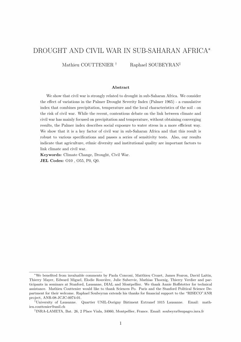
The inputs of the Palmer index are temperature, precipitation and the available water ca-

pacity of the soil. This contrasts with previous studies that looked at the impact of precipitation

and/or temperature on the risk of conflict (e.g. Miguel et al. 2004, Burke et al. 2009). Time

series show that PDSI and rainfall generally vary in opposite directions (see Figure 3) and

that PDSI and temperature generally vary in the same direction (see Figure 4). Rainfall (with

lags) explains 50% of the PDSI variation12 and 70 − 85% of the within-country PDSI varia-

tion.13 Temperature (with lags) explain 60% of the PDSI variation14 and 50% to 80% of the

within-country PDSI variation.15 Temperature and rainfall together explain 60% of the PDSI

variation16 and 70% to 90% of the within-country PDSI variation.17 This is consistent with the

theoretical formula of the PDSI, which is based on precipitation, temperature and the available

water content of the soil. Notice that consistently with the Palmer model, we find that rainfall

decreases the PDSI, but less so during hot years (see Supplementary Table ST4).18

2.2 Data on Civil Wars

We use the latest UCDP/PRIO Armed Conflict Dataset (v4-2011), over the 1946 - 2010 period,19

where some errors have been corrected and the data has been extended compared to previous

versions. We also use data from the Correlates Of War (COW) as a robustness check of our

results (see Appendix D). We use the civil war incidence dummy variable, which is equal to 1

for years with a number of battle deaths greater than 1, 000, and 0 otherwise (we further discuss

our results for alternative coding such as the onset or intensity of civil war).

The UCDP/PRIO database includes two categories of civil conflict: internal and interna-

tionalized armed conflict. An internationalized civil armed conflict occurs between the gov-

ernment of a state and one or more internal opposition group(s) with intervention from other

states. An internal civil armed conflict occurs between the government of a state and one or

more internal opposition group(s) without intervention from other states. We follow Jensen

and Gleditsch (2009) who point out that internationalized civil armed conflicts should not be

included in the analysis20 and focus on internal conflicts.

10These values are the R2 of least square estimates of panel models including country fixed effects and/ or yearfixed effects. The estimates are not reported here.

11See Supplementary Table ST1 in Appendix A.12Estimates not reported here.13We run several regressions of the PDSI on rainfall and temperature with some lags (and we use two data

sources: the first one is the same as Hsiang et al. 2011 and the second one is the same as Ciccone 2011). Seecolumns 1 to 6 in Supplementary Table ST2 in Appendix A.

14Estimates not reported here.15See columns 7 to 12 in Supplementary Table ST2 in Appendix A.16Estimates not reported here.17See Supplementary Table ST3 in Appendix A.18We find that rainfall decreases the PDSI, and the interaction term between rainfall and temperature has a

positive effect.19available at http://www.pcr.uu.se/research/ucdp/datasets/ucdp prio armed conflict dataset/20They show that the estimated effect of economic growth on civil war is reduced compared to

7

The history of sub-Saharan Africa reveals that there were important political changes

throughout the 20th century. Many African countries were colonized before World War II

and decolonized after World War II and the process of decolonization and the emergence of new

states present a theoretical and empirical challenge. This raises questions about the inclusion

or exclusion of anti-colonial civil wars in the analysis. We follow Fearon and Laitin (2003) who

argue that there are ways to include anti-colonial civil wars,21 but that the most conservative

strategy is to focus on civil wars in independent African states and to exclude the colonial

period. Hence, the time frame we consider is the period from a country’s independence to the

most recent year in our data, 2005. For example, the time frame for Ghana starts in 1957, for

Mozambique and Angola in 1975, and for the former French colonies in 1960.22

3 Estimation Framework

To estimate the effect of drought on the incidence of civil war, our baseline equation is the

following:

Warit = βPDSIit + ηi + θit+ εit, (3)

whereWarit is the the index of civil war in country i at time t and εit is the error term. PDSIit is

our country-specific measure of drought. The parameter β captures the effect of country-specific

drought on the risk of civil war. We also include country fixed effects (ηi) and country time

trends (θit) in our preferred specification. They serve as substitutes for variables which are

suspected of being endogenous (e.g. GDP), to control for unobserved heterogeneity, and to take

account of temporal trends in the causes of conflicts. We do not add other control variables to

the model in order to avoid the “bad control” problem (see Angrist and Pischke 2009).23

To give some insights into potential channels through which drought may affect the risk of

civil war (e.g. economic development, agricultural production, fractionalization indices, political

indices, food prices, etc.), we estimate the following equation:

yit = γPDSIit + yit−1 + ηi + θit+ ζit, (4)

Miguel et al. (2004)’s findings. They argue that according to Fearon and Laitin (2003), negative economicshocks should decrease the capacity of governments to send troops to civil wars in other states.

21The first way to code the data is to consider Ivory Coast as a single “state” for the whole 1946-2005 period(in fact it was part of the French empire from 1895 to independence in 1960). “States” that did not exist (suchas “Ivory Coast” from 1946 to 1960) are considered and the colonial empires are ignored. The second strategyis to consider colonial empires. For instance, Ivory Coast and Cameroon are categorized as belonging to theFrench empire before they gained independence (in 1960). Considering colonial empires requires the constructionof explanatory variables for whole empires. Fearon and Latin (2003) conclude that, although possible, it wouldbe very problematic to code variables such as GDP, ethnic fractionalization and democracy score. Also, in ourcontext it makes little sense to assign a climate value to a whole colonial empire. For instance, it would bemeaningless to assign the PDSI value of the French metropole (colonizer) to French colonies (such as Ivory Coastand Cameroon), or to assign the value of the PDSI averaged over the whole French empire to French colonies.

22Since different countries have different independence years, we have an unbalanced sample. However, we showthat our results are not influenced by this. In Supplementary Table ST5 (in Appendix A), column 1 shows ourbaseline estimates and column 2 shows the estimates of the same specification adjusted with sampling weights(weights that denote the inverse of the probability that the observation is included because of the samplingdesign): the significance of the effect is still 99% of confidence and the coefficient increases from 0.677 to 0.969.

23See section 3.2.3. Many variables that we may want to add are themselves outcome variables of droughtvariations. For instance, we know that drought affects GDP per capita (see Dell et al. 2012). The estimatedcoefficient of the PDSI will capture the effect of drought on the risk of civil war for a given level of GDP percapita. The problem is that this is not a causal argument.

8

where, yit is the country-specific measure of the potential channel, PDSIit our measure of

drought, yit−1 the lagged dependent variable (see Miguel et al. 2004), ζit is the error term, ηi

the country fixed effect and θit the country-specific time trend.

To investigate the underlying mechanisms, we include interaction terms between drought

and country-specific characteristics (time-invariant or time-varying) in the right-hand side set

of explanatory variables of equation 3. These interaction terms capture the effect of latent

tensions and shed light on factors that create a spark which fuels tensions and can lead to civil

conflicts. Denoting Ci the country characteristic, we estimate:

Warit = δPDSIit + λPDSIit × Cit + ρCit + ηi + θit+ ξit, (5)

where ξit is the error term. The parameter δ captures the mean effect of drought and parameter

λ captures the differentiated effect of drought on the risk of civil war according to the country

characteristic.

As our index of civil war is a dummy, we could have used a logit model. However, we

have preferred to consider the linear probability model throughout the paper and to report

the estimated effects using least squares. On the one hand, the logit methodology is undoubt-

edly preferable to the linear probability model if we want predictions with more than marginal

changes in the variables. On the other hand, as argued by Wooldridge (2002) the linear proba-

bility model (in binary response models) should be seen as a convenient approximation to the

underlying response probability. All in all, the linear probability model does not always predict

values within the unit interval, but it is usual and it seems a convenient approximation in our

case. One of the advantages of the linear model is that it enables us to use econometric tools to

take into account serial correlation and spatial autocorrelation in the climate data. Moreover,

some studies (e.g. King and Zeng 2001) claim that logit and probit may provide biased esti-

mates when used with data such as civil wars, because the number of events is relatively small

(5.4% of civil war in our sample).

An important issue is the estimation of the significance of the effects. As mentioned before,

since we use climate data, serial correlation within countries and spatial correlation between

countries have to be corrected when we estimate the standard errors. We follow Hsiang (2010)

and deal with the two problems simultaneously in all our regressions, using a nonparametric

estimation of the variance-covariance matrix for the error term allows both for cross-sectional

spatial contemporaneous correlation and country-specific serial correlation. Weights in this

matrix are uniform up to a cutoff distance of 1, 000 km (Conley 1999). Linear weights that fall to

zero after a lag length of 4 years are used to take serial correlation into account (Conley 2008).24

24We checked for the sensitivity of our baseline estimates to the distance cutoff of 1,000 km and to thelag length cutoff. We considered different cutoffs, from 2 to 10 years for the temporal dimension and1,000km/2,500km/5,000km for the spatial cutoff. Supplementary Table ST6 reports the standard errors forthe various possible combinations of the cutoff values (we do not report the coefficient, which is 0.677). We alsoused a two-way clustering method to compute the standard errors (Cameron et al. 2011).

9

4 Empirical Results

4.1 Main Results

Table 2 presents our main results. First, we run a model with country fixed effects (column

1). Drought has a positive effect on the within variation of the probability of civil war. In

column 2, we run a standard difference-in-difference model with the inclusion of year fixed

effects. The PDSI is no longer significant (p-value = 0.16). However, year fixed effects might

soak up a lot of the variation of interest, as they capture many factors that can influence the

incidence of conflict (e.g. a natural resource price shock) and variations in the global climate

(Hsiang et al. 2011). We then follow the literature25 and include country time trends instead

of year fixed effects (column 3). We show that the effect of the PDSI on civil war is significant

at the 99% level of confidence. A one standard deviation increase in the PDSI increases the

annual risk of conflict by an additional 1.7% (the standard deviation of the PDSI is 0.025, see

Table 1). Note that in terms of Palmer’s classification, a one standard deviation increase in

drought may correspond to a change from a near normal climate (PDSI between −0.005 and

0.005) to a moderate drought (0.02 to 0.03). A greater change in climate such as a change from

normal (PDSI = 0) to extremely dry (PDSI = 0.4) would increase the annual risk of civil war

by 2.7%.

Assuming that without PDSI variations (PDSI = 0, normal climate), the probability of

civil war evolves linearly, i.e. the probability of civil war is explained by country fixed effects

and country specific time trends, we find that the PDSI may have affected one-fifth (21%) of

all civil wars (in our sample).26 Our model explains 35% of the variance of the risk of civil war.

Using out-of-sample prediction, we find that the model explains 26% of the variance of the risk

of civil war out-of-sample.27 To illustrate our result, we have picked two cases. Figure 5 plots

the PDSI level and reports periods of conflict for Sudan and Uganda. The time series of PDSI

values for Sudan reached a peak in the early 80s and the civil war began in 1983; the time

series of PDSI values for Uganda shows two large peaks, one during the 80s and one around

2003-2005. These periods correspond precisely to two periods of civil war in Uganda. These

two cases illustrate a positive correlation between drought and the incidence of civil war.

4.2 Robustness of the Main Result

4.2.1 Sensitivity Tests

One of the criticisms of Miguel et al. (2004)’s seminal work is that the link between rainfall and

civil war fails to pass several sensitivity tests (see Buhaug 2010). In this section, we show that

our results are much less sensitive.

25See eg. Miguel et al. (2004), Jensen and Gleditsch (2009), Burke et al. (2009, 2010a), and Ciccone (2011).26We project the observed sequence of PDSI realizations onto our linear model (dWarij/dPDSI = 0.667) and

find 19 civil war years were associated with the PDSI: (β∑t

∑i

PDSIit) divided by the total number of civil

war years in the sample (88).27This percentage is computed using the following procedure. We estimate equation 3 using 1, 643 different

samples. Each observation is excluded once. Each set of estimates is used to compute a predicted value of therisk of civil war for the observation that was excluded from the sample. We then use the standard R-squaredformula and find 26%.

10

Supplementary Table ST7 (in Appendix A) shows the results of several sensitivity checks.

First, we relax the hypothesis of linearity of the country specific time trends and we augment

equation 3 with a country specific time trend squared term (column 1). The effect of the PDSI

remains significant at the 99% level of confidence. Second, we introduce a common linear time

trend and the effect of the PDSI is significant at the 95% (column 2); we then add a common

linear time trend squared and the effect of the PDSI is significant at the 99% (column 3).

Column 4 shows our estimates when the lagged civil war incidence is included in the right-hand

side of equation 3 and the effect of the PDSI remains significant.28 Column 5 finds that the

effect is still significant at the 99% level of confidence when we follow Hsiang et al. (2011) and

drop the observations for 1989 (the end of the Cold War) from our sample.

An important issue in the literature is the inclusion of lags of the climate variable. This

question seems less crucial in our context, as the PDSI is defined by a recursive formula and

then takes past PDSI values into account. However, to check whether our baseline specification

(Table 2, column 3) needs to be augmented with lagged (or forward) values of the PDSI, we

estimate equation 3 augmented with lagged or forward PDSI values. Supplementary Table ST8

contains our results. Column 1 replicates our baseline estimate (same as in Table 2, column 3).

Columns 2 and 3 augment the specification in column 1 with lagged PDSI values. Column 2

shows that the PDSI at time t− 1 has an insignificant effect on the contemporaneous incidence

of civil war. Column 3 shows that the effect of the PDSI at time t − 2 is also insignificant.

Columns 4 and 5 augment our preferred specification with forward PDSI values. Column 4

includes the PDSI at period t + 1 and finds that the effect is insignificant. Column 5 shows

that the effect of the PDSI at t + 2 is also insignificant. To check whether a sequence of dry

years is much worse than a single dry year, we add a term that interacts the current and the

lagged PDSI (column 6) and find that this variable has an insignificant effect on the risk of

civil war.29 Likelihood ratio tests also suggest that the inclusion of lags is not necessary. These

results strengthen our choice to use the contemporaneous PDSI value and no PDSI lags as our

preferred specification.

We also test the sensitivity of our results to a change in the time frame of the sample

considered. The processes of democratization and the development of sub-Saharan Africa might

have induced changes in the relationship between drought and civil war during the post-World

War II period. Thus, the effect of drought on civil war may be sensitive to the time frame in

our sample. We use our preferred specification and re-estimate the effect of the PDSI on civil

war for each time interval of a minimum of 20 consecutive years (i.e. 861 estimates) between

1965 and 2005. The graph at the top of Figure 6 shows the sign of the PDSI coefficient (β) for

every possible start and end year in the time scale. Pale grey represents negative values and

black represents positive values of the estimated effect of the PDSI. In most cases, the value

of the estimated PDSI coefficient is positive. The graph at the bottom of Figure 6 shows the

28The results are not affected when we use a General Method of Moment (GMM) to estimate this dynamicequation (Wooldridge 2002, page 304 or Greene 2002, page 308).

29We also considered two alternative measures of drought. First, we computed the intra-annual PDSI variationfor each country (moments of order 1, 2 and 3). Second, we considered spatial PDSI variations within eachcountry by computing various moments of the PDSI using the 2.5 degree x 2.5 degree grid cell year averages(within year variation is eliminated). In both cases, the effect of the PDSI is positive and significant, but thehigher moments of the PDSI are insignificant.

11

significance of the estimated PDSI coefficient (whether significant at the 5% level of confidence

or not). The PDSI coefficient is most often positive and significant, but it is negative and

non-significant when the time scale ends early. This result may be due to the small number

of ongoing civil wars and to the high frequency of “normal” climatic conditions before the 80s

(there are 28 observations with Warit = 1 before 1980 in our sample; see Figure 2 for the

frequency of a “normal” climate). Overall, our result is very robust to a change in the time

frame, compared to estimates that use rainfall and temperature data.30

Even if our sample is larger than in previous studies, our result might be sensitive to the in-

clusion/exclusion of a small number of observations.31 Figure 7 shows a plot of our observations

and the two and the three standard error limits (the 2-sigma and the 3-sigma outliers are the

observations outside the “2 s.d.” and “3 s.d.” limits, respectively). Supplementary Table ST13

shows our results using our preferred specification with different samples. Column 1 reports

our estimates over the whole sample (identical to column 3 in Table 2), column 2 shows our

estimates over a sample without the 3-sigma outliers and column 3 shows our estimates over

a sample without the 2-sigma outliers. The effect of the PDSI is lower than in our baseline

estimates, but it remains significant at the 99% level of confidence.32

So far, we have made implicit the assumption that the response of the risk of civil war to

the PDSI is linear. We relax this assumption and first include the square of the PDSI in the

right-hand side of equation 3. We find that the effect of this additional variable is insignificant

(estimates are not shown here). Second, we use a non-parametric estimate of the effect of the

PDSI (see for instance Deschenes and Greenstone 2011): we compute the 10 deciles of the PDSI

and run our preferred specification , including a variable for each of the 2nd to the 10th decile

of the PDSI (9 bins, with the first decile being our reference). Figure 8 plots the estimated

response function linking civil war and the nine PDSI bin variables. The Figure also plots the

coefficients plus and minus two standard errors. Our response function increases slightly for

the last bins, meaning that the effect of the PDSI on the risk of civil war is greater for the

highest PDSI values, i.e. for PDSI values which are classified as moderate drought or drier

according to Palmer’s classification (above the 8th decile of the PDSI distribution, i.e. for a

PDSI > 0.027). Overall, the magnitude of the effect is such that PDSI values above the first

decile are associated with a 5% to 7% additional risk of civil war. A one standard increase in

the PDSI (from a normal climate) translates into a 5% increase in the risk of civil war, which

is slightly greater than in our baseline estimates (1.7%).

30See the discussion of Buhaug et al. (2010) on Burke et al. (2010a). Notice that our results are robust to theusual time frame of Miguel et al. (2004): 1981 - 1999.

31Buhaug et al. (2010) argue that the estimates in Burke et al. (2010a) regarding temperature data do notpass this test.

32We also use the dfbeta statistic for the PDSI to identify observations that are likely to exercise an overlylarge influence (see Buhaug et al. 2010). It measures the impact of each observation on the estimated effect of acovariate. The critical value is 2/

√n, where n is the number of observations. We find a threshold that amounts to

.05 and identify 74 observations with higher dfbeta values. When these observations are excluded, the estimatedPDSI coefficient is lower and less significant; however, it remains significant at the 10% level. This confirms therobustness of the effect of drought for the post-colonial period (see Supplementary Table ST13, column 4).

12

4.2.2 Other Climate Variables

In this section, we compare the effect of the PDSI to the effect of rainfall and temperature on

the risk of civil war.

Supplementary Table ST9 presents our estimates of the effects of the PDSI and rainfall on

civil war. We estimate equation 3 augmented with rainfall levels or rainfall growth measures.

We use the same rainfall data as Hsiang et al. (2011) (columns 1 and 2) and a second data set

with the same rainfall data as Ciccone (2011) (columns 3 to 6). Columns 1 and 3 present our

estimates of equation 3 augmented with contemporaneous rainfall and one lag. The effect of

the PDSI is significant at the 95% and 90% level of confidence, respectively, whereas the effect

of rainfall is insignificant. Columns 2 and 4 show our estimates when a two-year lag is added

and find that the effect of the PDSI is generally less significant. However, the effect of rainfall

remains insignificant. In columns 5 and 6, we augment equation 3 with the contemporaneous

growth of rainfall and one lag, respectively (as in Miguel et al. 2004). In both cases, the effect

of the PDSI is significant (at the 90% and 95% level of confidence, respectively). However,

the effect of rainfall growth is insignificant. Supplementary Table ST10 presents our estimates

of the effects of the PDSI and temperature on civil war. We use equation 3 augmented with

temperature measures. We use contemporaneous temperature (column 1), then we add one lag

(column 2), and finally we add two lags (column 3). The effect of the PDSI is always significant

at the 99% level of confidence and the effect of temperature is generally insignificant. To check

whether a large fraction of the effect of the PDSI is due to global climate variations such as

ENSO (see Hsiang et al. 2011), we include various measures of El Nino fluctuations in our

baseline specification. Supplementary Table ST11 contains our results. The effect of the PDSI

is always positive and significant at the 99% level of confidence. This is another argument in

favor of the complementarity of our analysis with Hsiang et al. (2011).

Thus, our results show that the effect of the PDSI is robust to the inclusion of other local

climate measures (rainfall and temperature) and to global climate fluctuations (various measures

of ENSO). They also confirm the predictive power of the PDSI regarding civil wars.

4.2.3 Onset and Intensity of Civil War

A usual alternative measure of civil war is the onset (or outbreak) of civil war index. It is set

at 1 for the first year of civil war, set to missing for the subsequent civil war years, and at

0 for peace years.33 Supplementary Table ST12 shows our results. The PDSI has a positive

and significant effect on the probability of the outbreak of civil war if we only include country

fixed effects (column 1). However, columns 2 and 3 show that the PDSI has a non-statistically

significant effect on the onset of civil war when year fixed effects or country time trends are

included, respectively, suggesting that the PDSI is not a strong predictor of the onset of civil

war index.

To investigate whether the PDSI affects the intensity of civil war, we use two different

strategies. First, we test whether the effect of the PDSI is sensitive to a change in the battle-

33We take multiple contemporaneous conflicts in the same country into account. In our sample, there is onlyone country with two contemporaneous civil wars: PRIO data report that Ethiopia has experienced severalcontemporaneous civil wars. The onset index is then set to 1 for Ethiopia in 1976, 1980 and 1981.

13

related death threshold. We re-code our dependent variable Warit for each threshold between 25

and 200, 000 battle-related deaths per year and re-estimate our preferred specification. Figure 9

reports the value of the estimated coefficient of the PDSI (and the 95% interval of confidence).

The PDSI has a positive and robust effect on civil war as long as the battle-death threshold is at

least 1, 000. The coefficient of the PDSI is positive for thresholds between 25 and 999 (number

of battle deaths each year), but not significant in most cases. The 1, 000 battle-related death

threshold corresponds perfectly to the usual limit considered in the literature to distinguish

between civil war and civil conflict. However, we cannot assert whether this threshold we find

is due to a real phenomenon or to a variation in the precision of the data. It remains that the

effect of the PDSI on civil war is positive and significant at the 95% level of confidence, no

matter the battle-death threshold we consider.34

Second, we maintain the same set of explanatory variables as in equation 3, but we replace

the left-hand side dependent variable with different measures of the intensity of civil war. Sup-

plementary Table ST14 contains our estimates. We use three different approximations for the

number of battle deaths: a lower bound, a higher bound and the “best” estimates (according to

the PRIO data set). We also alternatively use the square root of the number of battle deaths

or the number of battle deaths. Columns 1, 4 and 7 contain our results when the left-hand-side

dependent variable is the square root of the number of battle deaths. In all cases, the PDSI

increases the intensity of civil war and the effect is significant at the 99% level of confidence.

Columns 2, 5 and 8 report our results when the left-hand-side dependent variable is the number

of battle deaths. Column 2 shows our results for the lower bound measure. Our results indicate

that a one standard deviation increase of the PDSI leads to 180 additional battle deaths and

the effect is significant at the 99% level of confidence. Column 5 reports our estimates for the

higher bound measure. We find that a one standard deviation increase of the PDSI leads to 800

additional battle deaths and the effect is significant at the 99% level of confidence. Column 8

shows our results for the “best” measure. Our estimates show that a one standard deviation

increase of the PDSI leads to 114 additional battle deaths and the effect is significant at the 95%

level of confidence. Columns 3, 6 and 9 show our estimates when the left-hand-side variable is

the number of battle deaths, but we use a Poisson regression instead of least squares in order

to account for the discrete nature of the dependent variable and the presence of a large number

of 0. Again, the PDSI has a positive effect on the number of battle-related deaths. The effect

is significant at the 99% level of confidence.

4.3 Channels and Other Outcome Variables

To provide insights into the potential channels through which drought affects the risk of civil

war, we look at whether the PDSI affects other economic and political outcomes. Blattman

and Miguel (2010) argue that drought may increase the risk of civil war because it decreases

the opportunity cost of fighting among rural populations; however, crop failure may also reduce

government revenues and/or state capacity. We first present estimates of the effect of the PDSI

on various measures of economic productivity and production. Table 3 contains our findings

34The effect becomes non-significant for thresholds higher than 50,000 deaths per year, but in that case only2 observations are still considered as civil war years.

14

regarding the effect of the PDSI on agricultural and total economic production, and different

measures of government finances.35

We use the specification of equation 4 where (log of) cereal yields (tons/ha) is the left-hand-

side variable (column 1). The PDSI has a negative and significant impact on cereal yields,

as expected, and the effect is significant at the 95% level of confidence. We show the PDSI

reduces agricultural income per capita (column 2). A one standard deviation increase in the

PDSI leads to a 1.5% decrease in agricultural income per capita and the effect is significant

at the 95% level of confidence. Column 3 shows that a one standard deviation increase in the

PDSI leads to a 2.2% increase in local food prices and the effect is significant at the 99% level

of confidence. These three results show that the PDSI has a considerable effect on agricultural

outcomes. This is consistent with previous studies that documented the significant impact

of other climate measures such as temperature, precipitation and El Nino variations on crop

yields (e.g. Schlenker and Lobell 2010 and Hsiang et al. 2011). These results suggest that an

opportunity cost mechanism may explain the effect of drought on civil war, through the negative

effect of drought on agricultural production.

In columns 4 and 5, we report the effect of drought on the global economic activity. The PDSI

has a negative and significant effect both on GDP per capita and economic growth (columns 4

and 5, respectively). Our results indicate that a one standard deviation increase in the PDSI

leads to a 0.66% decrease in GDP per capita and to a 0.5 decrease in economic growth (that

is 14% of the average).36 These results are consistent with recent but growing evidence that

climate affects economic performance (Hsiang 2010, Barrios et al. 2010, Zivin and Neidell 2010,

Jones and Olken 2010 and Dell et al. 2012).37

To test whether state capacity is also a channel for the drought-civil war relationship,

we present estimates of the effect of the PDSI on various measures of government finances

(columns 6 to 10 in Table 3). Column 6 uses the specification of equation 4 to explain tax

revenue (% of GDP) as a function of the PDSI. We find that a one standard deviation increase

of the PDSI increases tax revenue by 0.6% of GDP, and the effect is significant at the 99% level

of confidence. We find that the PDSI has an insignificant effect on government revenue (% of

GDP) (column 7). Columns 8 and 9 present the effect of the PDSI on government consumption

expenditure (% of GDP) and government consumption (% of GDP per capita), respectively.

We find that the PDSI has no significant effect on either measure of government consumption.

We also show that the PDSI has no significant impact on the level of military expenditures

(column 10). Overall, among the various measures of government finances we used, the ratio of

tax revenue over GDP is the only one that has a significant (and positive) effect on the risk of

civil war. An increase in collected tariffs due to an increase in imports (e.g. compensating for a

drop in agricultural production) may explain this result. This suggests that drought has little

35See Appendix C for a description of dependent variables.36The average growth is 3.6% over our sample.37Hsiang (2010) looks at temperatures and cyclones and shows that they negatively affect economic output.

Barrios et al. (2010) look at agriculture and hydro-energy supply as two channels through which rainfall is likely tohave adversely affected the development of sub-Saharan Africa. Zivin and Neidell (2010) show that temperatureshave an impact on U.S. workers’ allocation of time. Jones and Olken (2010) show that temperatures reduce theexports of poor countries. Dell et al. (2012) show that temperature shocks reduce growth in poor countries (aswell as agricultural output, industrial output, and political stability).

15

or no effect on state capacity.38

Democratic change is an important political outcome related to civil wars. Bruckner and

Ciccone (2011) have shown that country-specific variations in rainfall are followed by significant

improvements in the democratic institutions of sub-Saharan African countries. Table 4 links the

PDSI to various indices of democratic change. We use the same specification as in equation 3,

but the left-hand-side outcome variable is a democratic change index instead of a civil war index.

From column 1 to column 9, we successively use 9 different indices of democratic change (see

Appendix C for a description of the indices). Column 1 shows that a one standard deviation

increase in the PDSI raises the variation in the polity score by 0.17 (the average variation being

0.07), and the effect is significant at the 95% level of confidence. Column 5 shows that a one

standard deviation increase in the PDSI raises the risk of a coup d’etat by an additional 2.4%,

and the effect is significant at the 90% level of confidence. Column 9 indicates that drought has

a positive effect on the democratization step. These results confirm the main result of Bruckner

and Ciccone (2011), which is that drought is followed by a democratic improvement. However,

we find that the PDSI has an insignificant effect on the variation in executive recruitment

(column 2), on the variation in political competition (column 3), on the variation in executive

constraint (column 4), on the occurrence of a coup d’etat in a democracy (column 6), on

democratic transition (column 7), and on autocratic transition (column 8).

4.4 Interaction between PDSI and Country Characteristics

The effect of drought on civil war may be due to latent tensions and drought may create a

spark which fuels tensions and may lead to the outbreak of civil conflicts. To investigate the

potential underlying mechanisms linking drought to civil war, we consider interactions between

drought and country characteristics. Various country characteristics may channel the effect of

drought on the risk of civil war. Table 5 contains our estimates of equation 5 on the effect of

the interactions between the PDSI and various country characteristics.

The development interaction result (we use the log GDP per capita in 1965 in order to avoid

reverse causality problems, column 1) indicates that relatively poor countries hit by drought

are as prone to civil war as relatively rich countries. This result differs from the (worldwide)

cross-country evidence that poor countries are more prone to conflict (Fearon and Laitin 2003),

but this is certainly due to our focus on sub-Saharan Africa and the fact that this region of the

world was relatively homogeneous in terms of economic conditions in 1965.

In column 2, we interact our measure of the PDSI with a measure of ethnic fractionalization.

Interestingly, we find that the effect of the interaction term is significant and positive: countries

which are relatively more ethnically fractionalized and are hit by a drought are more prone to

conflict than countries with less ethnic fractionalization (the total estimated effect is negative

for three countries with a low fractionalization in the sample - Equatorial Guinea, Lesotho,

and Swaziland). We also test for the effect of interaction terms between drought and linguistic

or religious fractionalization, but we find no significant results (we have not reported these

estimates). The role of ethnic groups in conflicts39 is a contentious issue and the debate is still

38The interpretation of these results need to be taken with caution because of the small sample size for somespecifications.

39Fearon (2006) reports that 709 minority ethnic groups are identified around the world and that at least 100

16

very active.40 This result contrasts with cross-country studies that find that ethnic diversity is

not significantly correlated to conflict across countries (Easterly and Levine 1997, Collier and

Hoeffler 1998, 2004 and Fearon and Laitin 2003). However, our result is consistent with recent

studies by Esteban et al. (2012a,b) who show (theoretically grounded) cross-country evidence

that civil conflict is correlated with ethnic polarization and fractionalization.41

In column 3, we test for the effect of an interaction term between drought and the percentage

of mountainous terrain in a given country. The interaction term is positive and significant. We

find that countries with a relatively higher percentage of mountainous terrain suffering from

drought are more prone to conflict than countries with a lower percentage of mountainous ter-

rain. This result is consistent with previous studies that found that mountainous terrain is a

correlate of civil war (Collier and Hoeffler 1998, 2004, and Fearon and Laitin 2003). We also

interact the PDSI with the population density in 1965 and find a positive effect, as expected,

but the effect is not significant. Again, this result contrasts with cross-country studies that

report a robust correlation between conflict and the size of the population (see Hegre and Sam-

banis 2006). In other words, we do not find evidence supporting the Malthusian view according

to which population pressure leads to resource scarcity and environmental degradation (see

Homer Dixon 1999 for a review). In columns 5 to 8, we interact the PDSI with indices of the

level of democracy. In column 5, we include an interaction term between the PDSI and the

aggregated level of democracy (polity score) and find that relatively democratic countries hit

by a drought are more prone to civil war than relatively autocratic countries. In columns 6, 7

and 8, we include an interaction term of the PDSI and three different indices of democracy: the

executive recruitment level, the level of political competition, and the level of executive con-

straint, respectively. The democracy interaction results indicate that countries with a relatively

low level of democracy which are hit by a drought are more prone to civil war than countries

with a relatively high level of democracy.

Another empirical strategy to investigate the potential underlying mechanisms linking drought

to civil war is to estimate the effect of drought on civil war on sub-samples split by country char-

acteristics. We focus on the agricultural share of GDP, GDP per capita, and ethnic and linguistic

fractionalization. For each of these variables, we plot the estimated coefficient (black curve)

and the 95% of confidence interval (see Figures 10 to 13). The x-axis represents the cutoffs of

the variable of interest used to define the sub-sample (cutoff of the agricultural share of GDP,

GDP per capita or ethnic fractionalization). The model is re-estimated for each sub-sample

from which the country with the lowest value is excluded, and countries are also excluded with

respect to increasing values for this variable. Our results show that countries with a relatively

large agricultural sector which are hit by a drought are more prone to civil war (Figure 10).42

Figure 11 presents the results when we split the sample based on GDP per capita in 1965. It

had members who engaged in an ethnically-based rebellion against the state between 1945 and 1998.40Blattman and Miguel (2010) provide a summary of the debate between “primordialists” (Horowitz 1985) and

“modernists” (Bates 1986 and Gellner 1983) who argue that ethnic conflict arises when groups excluded fromsocial and political power begin to experience economic modernization.

41Esteban et al. (2012a,b) also argue that ethnic conflicts are likely to be instrumental, rather than driven byprimordial hatreds.

42Note that the slight decrease for an agricultural share above 50% is notably due to the small size of thesample.

17

indicates that drought has a similar impact on the risk of civil war in relatively developed coun-

tries and in relatively less developed countries, except for the richest countries in the sample.

Figure 12 and Figure 13 suggest that relatively ethnically and linguistically diverse countries

hit by a drought are more prone to civil war than relatively ethnically and linguistically uniform

countries, respectively.

5 Conclusion

In this paper, we have used a meteorological measurement of drought, the Palmer Drought

Severity Index, with values computed according to a supply and demand model of soil moisture.

We have shown that drought (PDSI values) and the incidence of civil war are positively and

robustly linked for the independent sub-Saharan African countries. Furthermore, as discussed,

our analysis cannot be subjected to the criticisms leveled at studies that rely on rainfall and

temperature data, and we have shown that our results pass several sensitivity tests.

Our results suggest that drought is a key factor in security issues and that there are sev-

eral pathways through which climate variations may increase the risk of civil war. First,

consistently with recent evidence that civil conflict is associated with ethnic diversity (Este-

ban et al. 2012a,b), our results suggest that drought and ethnic diversity are interacting roots

of civil war. Second, we also find that democracy reduces the negative effect of drought on

civil war. Third, we find that agricultural production may play a part in the link between

drought and civil war. This result is consistent with growing evidence that the climate affects

economic performance (Schlenker and Roberts 2006, Hsiang 2010, Barrios et al. 2010, Jones

and Olken 2010, Schlenker and Lobell 2010, Zivin and Neidell 2010 and Dell et al. 2012), which

may in turn affect the risk of conflict (Miguel et al. 2004). African countries remain highly

dependent on agriculture for both employment and economic production, with agriculture ac-

counting for up to more than 60% of their gross domestic product.43 Lobell et al. (2008) and

Schlenker and Lobell (2010) show that increases in temperature and decreases in precipitation

have strong negative effects on staple crop production. Their projections indicate that Africa

is one of the regions in the world where the climate will be the most affected. As argued in

Burke et al. (2010b), the negative effects of climate fluctuations on agricultural productivity

and their importance for economic performance should push governments and aid agencies to

help the African agricultural sector face climate change. Burke et al. (2010b) suggest several

strategies to mitigate the effect of climate change on the likelihood of conflict. Those strategies

include technical solutions such as developing new crop varieties adapted to a drier climate,

to build irrigation infrastructures and to improve existing ones (World Bank 2007). They also

include mechanisms such as the development of insurance against catastrophic weather risk

events (Hess et al. 2005) to compensate for weak primary insurance markets. Miguel (2007)

suggests making international aid contingent on climate risk to prevent the emergence of violent

acts. Our results also suggest that on of the channels between climate and civil war is economic

performance in the agricultural sector.

43See World Bank (2011), World Development Indicators 2011. Available at: www.worldbank. org/data/.Accessed on December 15, 2011.

18

Tables

Table 1: Descriptive Statistics of PDSI

Country Mean PDSI SD PDSI Max PDSI Min PDSI # of stations

Angola .0071984 .0107785 .0274556 -.019194 216Benin .0411368 .03853 .1165667 -.036375 12

Botswana .0130075 .0248074 .0460139 -.0636972 108Burkina Faso .0345842 .0264598 .0965361 -.0195167 36

Cameroon .0205576 .0254717 .102646 -.019745 60Central. Afr. Rep .0164558 .0200309 .0598714 -.0265631 84

Chad .0147019 .014445 .0437842 -.0192711 228Congo .0029642 .0181206 .0462563 -.0263271 48

Dem. Rep. Congo -.0017612 .0086887 .0165686 -.0321497 360Equatorial Guinea .0285614 .0219395 .0995095 -.0004417 24

Eritrea .0019821 .0168117 .0204083 -.0247667 24Ethiopia .0054814 .0146646 .0299699 -.0368096 156Gabon .0104718 .0267633 .0933485 -.0452917 36Ghana .0253675 .0333554 .0830083 -.0424792 24

Guinea Bissau .0277526 .0261821 .0700375 -.0177313 48Ivory Coast .0286724 .0271378 .0729271 -.0381312 48

Kenya .0021568 .0196988 .0297635 -.0581708 96Lesotho .011265 .021537 .0538083 -.0356417 12Liberia .0189005 .0248124 .0721667 -.0319333 12

Madagascar .0037987 .014909 .0405948 -.0283302 96Malawi .0184314 .0290299 .097125 -.0272625 24

Mali .0191649 .0143314 .0484657 -.0060814 204Mauritania .0195388 .0120298 .0421617 -.0099106 180

Mozambique .0175786 .0205434 .0653042 -.016535 120Namibia .013263 .0106717 .0294477 -.0024326 132

Niger .0164668 .0146296 .0462526 -.0098866 192Nigeria .0232486 .0228473 .0727674 -.0195644 132Senegal .0344408 .0242616 .0745833 -.0158917 36

Sierra Leone .0244459 .0221126 .074225 -.019175 12Somalia .0021149 .0122863 .0198657 -.0420463 108

South Africa .008476 .0167565 .0388681 -.0440833 216Sudan .0204686 .0185983 .061752 -.0173794 408

Swaziland .0169079 .0298251 .0864917 -.0333917 12Togo .0206309 .0305059 .0749333 -.0614458 24

Tanzania -.0015626 .0161149 .0314391 -.0454378 156Uganda .0230863 .0308077 .0811417 -.0543583 48Zambia .0192661 .0264835 .0941342 -.0274933 120

Zimbabwe .028104 .0237525 .0756861 -.0209417 72

Total 0.0169 0.0247 0.1166 -0.0637 -

Note: This Table reports the mean, the standard deviation, the maximum and the minimum for PDSIvalues. We also report the number of stations for the measure of the PDSI. The descriptivestatistics are computed using the same sample as in our baseline estimates (Table 2, column 3).

19

Table 2: The Effect of Drought on Civil War

Specifications (1) (2) (3)Dep. Var. Civil War

PDSI 0.700*** 0.275 0.677***(0.149) (0.197) (0.201)

Country Fixed Effect Yes Yes YesTime Fixed Effect - Yes -Country Time Trends - - Yes

Observations 1,643 1,643 1,643R-squared 0.305 0.349 0.350

Note: Conley standard errors in parentheses with ∗∗∗, ∗∗ and ∗ re-spectively denoting significance at the 1%, 5% and 10% lev-els. The dependent variable comes from the UCDP/PRIOArmed Conflict Dataset v4-2011 over the 1946 - 2010 pe-riod. Civil War is a dummy which is equal to 1 for a num-ber of battle deaths greater than 1,000. It includes onlyinternal civil wars. PDSI is the Palmer Drought SeverityIndex. Column 1 includes country fixed effects. Column 2includes country and year fixed effects. Column 3 includescountry fixed effects and country time trends.

Table 3: The Effect of Drought on Different Outputs

Specifications (1) (2) (3) (4) (5)Dep. Var. ln Cereal Yield ln Agricultural ln Local Food ln GDP/cap GDP Growth

Income/cap Prices

PDSI -132.6** -0.577** 0.871*** -0.265** -21.04**(58.15) (0.222) (0.227) (0.0992) (8.502)

Observations 1,447 1,177 32,569 1,543 1,375R-squared 0.853 0.951 0.957 0.989 0.214

Specifications (6) (7) (8) (9) (10)Dep. Var. Tax Revenue Gov. Revenue Gov. Consumption Gov. Consumption Military

(% of GDP) (% of GDP) Expenditure (% of GDP) Share Expenditure

PDSI 24.23*** 11.03 6.428 2.918 -0.496(8.134) (12.15) (4.902) (3.221) (0.959)

Observations 150 150 1,333 1,543 476R-squared 0.981 0.982 0.866 0.960 0.961

Note: Robust standard errors clustered at country level in parentheses with ∗∗∗, ∗∗ and ∗ respectively denoting significanceat the 1%, 5% and 10% levels.PDSI is the Palmer Drought Severity Index.All specifications include country fixed effects and country time trends. Column 3 includes also product fixed effects.ln Cereal Yield and ln Agricultural Income/cap come from Hsiang (2011). ln local food prices comes from FAO. lnGDP/cap and GDP Growth come from Penn World Table 7.0. Tax Revenue, Government Revenue, GovernmentConsumption and Government Consumption Share come from World Development Indicator. See Appendix C forfurther details on the dependent variables.

20

Tab

le4:

Th

eE

ffec

tof

Dro

ugh

ton

Dem

ocr

atic

Ch

ange

Sp

ecifi

cati

ons

(1)

(2)

(3)

(4)

(5)

(6)

(7)

(8)

(9)

Dep

.V

ar.

∆P

olity

∆E

xec

uti

ve

∆P

oliti

cal

∆E

xec

uti

ve

Coup

Coup

inD

emocr

ati

cA

uto

crati

cD

emocr

ati

zati

on

Rec

ruit

men

tC

om

pet

itio

nC

onst

rain

tdem

ocr

acy

transi

tion

transi

tion

Ste

p

PD

SI

6.7

56**

-3.5

79

-2.7

95

-2.0

37

0.9

42*

-0.3

11

-0.1

66

0.8

01

0.6

85***

(3.3

74)

(23.8

7)

(23.8

8)

(24.3

6)

(0.5

12)

(0.2

35)

(0.2

92)

(0.7

45)

(0.2

57)

Obse

rvati

ons

1,5

50

1,5

52

1,5

52

1,5

52

1,6

43

1,6

43

1,1

02

467

1,4

74

R-s

quare

d0.0

46

0.0

08

0.0

08

0.0

08

0.2

35

0.1

19

0.1

41

0.6

92

0.4

58

Note

:C

on

ley

stan

dard

erro

rsin

pare

nth

eses

wit

h∗∗∗,∗∗

an

d∗

resp

ecti

vel

yd

enoti

ng

sign

ifica

nce

at

the

1%

,5%

an

d10%

level

s.A

llsp

ecifi

cati

on

sin

clu

de

cou

ntr

yfi

xed

effec

tsan

dco

untr

yti

me

tren

ds.

PD

SI

isth

eP

alm

erD

rou

ght

Sev

erit

yIn

dex

.D

epen

den

tvari

ab

les

are

con

stru

cted

than

ks

toP

olity

IVd

ata

.∆

Polity

cap

ture

sth

evari

ati

on

of

the

polity

score

fromt

tot

+1.

∆Execu

tive

Recru

itmen

tre

pre

sents

the

vari

ati

on

of

the

exec

uti

ve

recr

uit

men

tfr

omt

tot

+1.

∆PoliticalCompetition

rep

rese

nts

the

vari

ati

on

of

the

politi

cal

com

pet

itio

nfr

omt

tot

+1.

∆Execu

tive

Constraint

rep

rese

nts

the

vari

ati

on

of

the

exec

uti

ve

con

stra

int

fromt

tot

+1.Coup

isa

du

mm

yeq

ual

to1

ifth

ere

was

aco

up

ina

cou

ntr

yat

tim

et.

Coupin

Dem

ocracy

isa

du

mm

yeq

ual

to1

ifth

ere

was

aco

up

ina

dem

ocr

ati

cco

untr

yat

tim

et.

Dem

ocraticTransition

isa

du

mm

yco

ded

1if

aco

untr

yw

as

non

-dem

ocr

ati

cat

tim

et,

bu

td

emocr

ati

cat

tim

et+

1.AutocraticTransition

isa

du

mm

yco

ded

1if

aco

untr

yw

as

dem

ocr

ati

cat

tim

et

an

dn

on

-dem

ocr

ati

cat

tim

et+

1.Dem

ocratizationStep

isa

du

mm

yco

ded

1if

the

cou

ntr

yw

as

up

gra

ded

toei

ther

ap

art

ial

or

full

dem

ocr

acy

bet

wee

nt

an

dt

+1.

See

Ap

pen

dix

Cfo

rm

ore

det

ails.

21

Table 5: Interactions between Drought and Country Characteristics

Specifications (1) (2) (3) (4)Dep. Var. Civil War

PDSI 1.952 -0.807*** 0.141 0.486*(2.423) (0.274) (0.195) (0.286)

PDSI * ln GDP/cap ini. -0.246(0.480)

PDSI * Frac. Ethn. 2.130***(0.560)

PDSI * % Mountainous Terrain 0.395***(0.146)

PDSI * Pop Density ini. 0.00135(0.00138)

Observations 1,120 1,643 1,592 1,120R-squared 0.406 0.351 0.352 0.407

Specifications (5) (6) (7) (8)Dep. Var. Civil War

PDSI 0.829*** 0.683*** 0.684*** 0.667***(0.246) (0.190) (0.189) (0.192)

Polity t− 1 -0.000831(0.00135)

PDSI * Polity t− 1 0.0347(0.0337)

Executive Recruitment t− 1 0.0180(0.0169)

PDSI * Executive Recruitment t− 1 -0.00142**(0.000593)

Political Competition t− 1 0.0181(0.0169)

PDSI * Political Competition t− 1 -0.00142**(0.000593)

Executive Constraint t− 1 0.0190(0.0168)

PDSI * Executive Constraint t− 1 -0.00143**(0.000593)

Observations 1,555 1,552 1,552 1,552R-squared 0.355 0.375 0.375 0.375

Note: Conley standard errors in parentheses with ∗∗∗, ∗∗ and ∗ respectively denoting significance at the1%, 5% and 10% levels. All specifications include country fixed effects and country time trends.PDSI is the Palmer Drought Severity Index. The dependent variable comes from the UCDP/PRIOArmed Conflict Dataset v4-2011 over the 1946 - 2010 period. Civil War is a dummy which is equalto 1 for a number of battle deaths greater than 1,000. It includes only internal civil wars. SeeAppendix C for more details on the independent variables.

22

Figures

Figure 1: Maps of PDSI

a. 1945-1960 b. 1960-1970

c. 1970-1980 d. 1980-1990

e. 1990-2005

This Figure represents the evolution of the PDSI over time. Deeper red indicates a drier climate (a higher PDSI level)

23

Figure 2: PDSI Density

02

46

81

0P

erce

nt

-.05 0 .05 .1 .15PDSI

1945 - 2005

01

02

03

04

0P

erc

ent

-.05 0 .05 .1 .15PDSI

1945 - 1960

05

10

15

20

Pe

rce

nt

-.05 0 .05 .1 .15PDSI

1960 - 1970

05

10

15

20

Pe

rce

nt

-.05 0 .05 .1 .15PDSI

1970 - 1980

05

10

15

Pe

rce

nt

-.05 0 .05 .1 .15PDSI

1980 - 1990

05

10

15

Pe

rce

nt

-.05 0 .05 .1 .15PDSI

1990 - 2005

Drought distribution by decades for Sub-Saharan Africa

Drought Distribution by decades

This Figure shows the distribution of the PDSI for the sub-Saharan region for the 1946-2005 period and its evolution over

the decades. A value of 0 refers to a “normal” climate, a value of +0.04 to an “extremely dry” climate, and a value of -0.04

to an “extremely wet” climate.

24

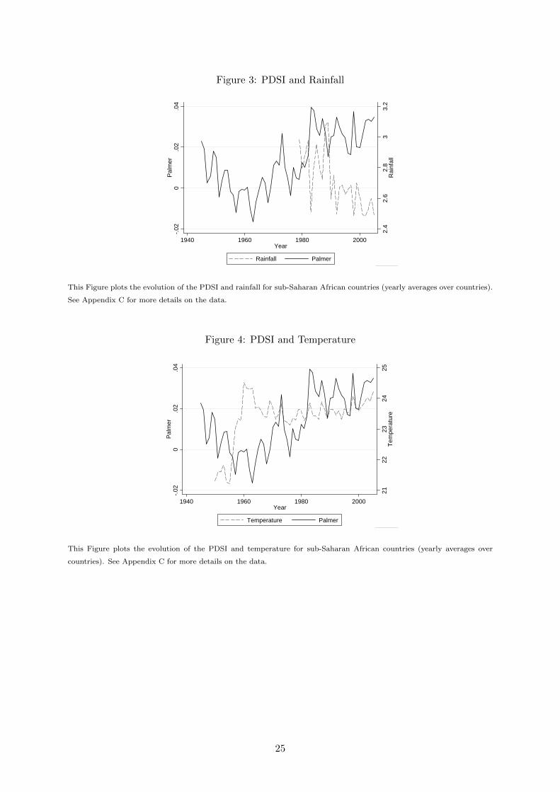
Figure 3: PDSI and Rainfall

-.02

0.0

2.0

4P

alm

er

2.4

2.6

2.8

33.

2R

ainf

all

1940 1960 1980 2000Year

Rainfall Palmer

This Figure plots the evolution of the PDSI and rainfall for sub-Saharan African countries (yearly averages over countries).

See Appendix C for more details on the data.

Figure 4: PDSI and Temperature

-.02

0.0

2.0

4P

alm

er

2122

2324

25T

empe

ratu

re

1940 1960 1980 2000Year

Temperature Palmer

This Figure plots the evolution of the PDSI and temperature for sub-Saharan African countries (yearly averages over

countries). See Appendix C for more details on the data.

25

Figure 5: Time Series of PDSI and Civil Wars for Sudan and Uganda-.

05

0.0

5.1

Pa

lme

r

1960 1970 1980 1990 2000 2010

Civil War Palmer

Sudan

-.0

50

.05

.1P

alm

er

1960 1970 1980 1990 2000 2010

Civil War Palmer

Uganda

The grey areas represent the years of civil war from the UCDP/PRIO Armed Conflict Dataset v4-2011 over the 1946 - 2010

period. Only internal civil wars are included. The y-axis reports the PDSI values. The black line represents the evolution

of the PDSI.

26

Figure 6: Drought Effect with Different Time Frame

194519501955196019651970197519801985

Sta

rt Y

ea

r

19

65

19

67

19

69

19

71

19

73

19

75

19

77

19

79

19

81

19

83

19

85

19

87

19

89

19

91

19

93

19

95

19

97

19

99

20

01

20

03

20

05

End Year

< 0

> 0

Size of Drought Coefficient

194519501955196019651970197519801985

Sta

rt Y

ea

r

19

65

19

67

19

69

19

71

19

73

19

75

19

77

19

79

19

81

19

83

19

85

19

87

19

89

19

91

19

93

19

95

19

97

19

99

20

01

20

03

20

05

End Year

NonSignifcant

Significant

Significance of Drought

The Figure shows (re-)estimates of our preferred specification (Table 2, column 3) for all possible time intervals of a

minimum of 20 consecutive years (i.e. 861 estimates). Each square represents the size of the coefficient of the PDSI ( β)

for every possible start and end year in the time scale. The graph at the bottom of the figure represents the degree of

significance of the estimated coefficient of the PDSI (whether significant at the 5% level of confidence or not).

27

Figure 7: Outliers

AGOAGOAGOAGOAGOAGOAGOAGOAGOAGOAGOAGOAGOAGOAGO

AGO

AGO

AGOAGOAGO

AGOAGOAGO

AGO

AGOAGOAGOAGOAGOAGOAGO

BENBENBENBENBENBENBENBENBENBENBENBENBENBENBENBENBENBENBENBENBENBENBENBENBENBENBENBENBENBENBENBENBENBENBENBENBENBENBENBENBENBENBENBENBENBENBFABFABFABFABFABFABFABFABFABFABFABFABFABFABFABFABFABFABFABFABFABFABFABFABFABFABFABFABFABFABFABFABFABFABFABFABFABFABFABFABFABFABFABFABFABFABWABWABWABWABWABWABWABWABWABWABWABWABWABWABWABWABWABWABWABWABWABWABWABWABWABWABWABWABWABWABWABWABWABWABWABWABWABWABWABWACAFCAFCAFCAFCAFCAFCAFCAFCAFCAFCAFCAFCAFCAFCAFCAFCAFCAFCAFCAFCAFCAFCAFCAFCAFCAFCAFCAFCAFCAFCAFCAFCAFCAFCAFCAFCAFCAFCAF

CAFCAFCAFCAFCAFCAFCAFCIVCIVCIVCIVCIVCIVCIVCIVCIVCIVCIVCIVCIVCIVCIVCIVCIVCIVCIVCIVCIVCIVCIVCIVCIVCIVCIVCIVCIVCIVCIVCIVCIVCIVCIVCIVCIVCIVCIVCIVCIVCIVCIVCIVCIVCIVCMRCMRCMRCMRCMRCMRCMRCMRCMRCMRCMRCMRCMRCMRCMRCMRCMRCMRCMRCMRCMRCMRCMRCMRCMRCMRCMRCMRCMRCMRCMRCMRCMRCMRCMRCMRCMRCMRCMRCMRCMRCMRCMRCMRCMRCMRCOGCOGCOGCOGCOGCOGCOGCOGCOGCOGCOGCOGCOGCOGCOGCOGCOGCOGCOGCOGCOGCOGCOGCOGCOGCOGCOGCOGCOGCOGCOGCOGCOGCOGCOGCOGCOGCOGCOGCOGCOGCOGCOGCOGCOGCOGERIERIERIERIERIERIERIERIERIERIERIERIERI

ETHETHETHETHETHETHETHETHETHETHETHETHETHETHETHETHETHETHETHETHETHETHETHETHETHETHETHETHETHETH

ETHETH

ETHETH

ETHETHETHETHETHETHETH

ETH

ETHETHETHETHETH

ETHETHETHETHETHETHETHETHETHETHETHETHETHETH

GABGABGABGABGABGABGABGABGABGABGABGABGABGABGABGABGABGABGABGABGABGABGABGABGABGABGABGABGABGABGABGABGABGABGABGABGABGABGAB

GABGABGABGABGABGABGABGHAGHAGHAGHAGHAGHAGHAGHAGHAGHAGHAGHAGHAGHAGHAGHAGHAGHAGHAGHAGHAGHAGHAGHAGHAGHAGHAGHAGHAGHAGHAGHAGHAGHAGHAGHAGHAGHAGHAGHAGHAGHAGHAGHAGHAGHAGHAGHAGHAGINGINGINGINGINGINGINGINGINGINGINGINGINGINGINGINGINGINGINGINGINGINGINGINGINGINGINGINGINGINGINGINGINGINGINGINGINGINGINGINGINGINGINGINGINGINGINGINGNQGNQGNQGNQGNQGNQGNQGNQGNQGNQGNQGNQGNQGNQGNQGNQGNQGNQGNQGNQGNQGNQGNQGNQGNQGNQGNQGNQGNQGNQGNQGNQGNQGNQGNQGNQGNQGNQKENKENKENKENKENKENKENKENKENKENKENKENKENKENKENKENKENKENKENKENKENKENKENKENKENKENKENKENKENKENKENKENKENKENKENKENKENKENKENKENKENKENKENLBRLBRLBRLBRLBRLBRLBRLBRLBRLBRLBRLBRLBRLBRLBRLBRLBRLBRLBRLBRLBRLBRLBRLBRLBRLBRLBRLBRLBRLBRLBRLBRLBRLBRLBRLBRLBRLBRLBRLBRLBRLBRLBRLBRLBR

LBR

LBRLBRLBRLBRLBRLBRLBRLBRLBRLBRLBRLBR

LBR

LBRLBRLSOLSOLSOLSOLSOLSOLSOLSOLSOLSOLSOLSOLSOLSOLSOLSOLSOLSOLSOLSOLSOLSOLSOLSOLSOLSOLSOLSOLSOLSO

LSOLSOLSOLSOLSOLSOLSOLSOLSOLSOMDGMDGMDGMDGMDGMDGMDGMDGMDGMDGMDGMDGMDGMDGMDGMDGMDGMDGMDGMDGMDGMDGMDGMDGMDGMDGMDGMDGMDGMDGMDGMDGMDGMDGMDGMDGMDGMDGMDGMDGMDGMDGMDGMDGMDGMDGMLIMLIMLIMLIMLIMLIMLIMLIMLIMLIMLIMLIMLIMLIMLIMLIMLIMLIMLIMLIMLIMLIMLIMLIMLIMLIMLIMLIMLIMLIMLIMLIMLIMLIMLIMLIMLIMLIMLIMLIMLIMLIMLIMLIMLIMLI

MOZMOZMOZMOZMOZMOZ

MOZMOZMOZMOZ

MOZMOZMOZMOZMOZMOZ

MOZ

MOZMOZMOZMOZMOZMOZMOZMOZMOZMOZMOZMOZMOZMOZMRTMRTMRTMRTMRTMRTMRTMRTMRTMRTMRTMRTMRTMRTMRTMRTMRTMRTMRTMRTMRTMRTMRTMRTMRTMRTMRTMRTMRTMRTMRTMRTMRTMRTMRTMRTMRTMRTMRTMRTMRTMRTMRTMRTMRTMRTMWIMWIMWIMWIMWIMWIMWIMWIMWIMWIMWIMWIMWIMWIMWIMWIMWIMWIMWIMWIMWIMWIMWIMWIMWIMWIMWIMWIMWIMWIMWIMWIMWIMWIMWIMWIMWIMWIMWIMWIMWIMWINAMNAMNAMNAMNAMNAMNAMNAMNAMNAMNAMNAMNAMNAMNAMNAMNERNERNERNERNERNERNERNERNERNERNERNERNERNERNERNERNERNERNERNERNERNERNERNERNERNERNERNERNERNERNERNERNERNERNERNERNERNERNERNERNERNERNERNERNERNER

NGANGANGANGANGANGANGA

NGANGANGANGA

NGANGANGANGANGANGANGANGANGANGANGANGANGANGANGANGANGANGANGANGANGANGANGANGANGANGANGANGANGANGANGANGANGANGANGA

SDNSDNSDNSDNSDNSDNSDN

SDNSDNSDNSDNSDNSDNSDNSDNSDNSDN

SDNSDNSDNSDNSDNSDNSDNSDNSDNSDN

SDNSDNSDNSDNSDNSDNSDNSDNSDNSDN

SDNSDN

SDNSDNSDNSDNSDNSDNSDNSDN

SDN

SDN

SDN

SENSENSENSENSENSENSENSENSENSENSENSENSENSENSENSENSENSENSENSENSENSENSENSENSENSENSENSENSENSENSENSENSENSENSENSENSENSENSENSENSENSENSENSENSENSENSLESLESLESLESLESLESLESLESLESLESLESLESLESLESLESLESLESLESLESLESLESLESLESLESLESLESLESLESLESLESLESLESLESLESLESLESLE

SLESLE

SLESLESLESLESLESLE

SOMSOMSOMSOMSOMSOMSOMSOMSOMSOMSOMSOMSOMSOMSOMSOMSOMSOMSOMSOMSOMSOMSOMSOMSOMSOMSOMSOM

SOM

SOM

SOMSOMSOM

SOMSOMSOMSOMSOMSOMSOMSOMSOMSOMSOMSOMSOM

SWZSWZSWZSWZSWZSWZSWZSWZSWZSWZSWZSWZSWZSWZSWZSWZSWZSWZSWZSWZSWZSWZSWZSWZSWZSWZSWZSWZ

SWZSWZSWZSWZSWZSWZSWZSWZSWZSWZTCDTCDTCDTCDTCDTCDTCDTCDTCDTCDTCDTCDTCDTCDTCDTCDTCDTCDTCD

TCD

TCDTCDTCDTCDTCDTCDTCDTCDTCDTCD

TCD

TCDTCDTCDTCDTCDTCDTCDTCDTCDTCDTCDTCDTCDTCDTCDTGOTGOTGOTGOTGOTGOTGOTGOTGOTGOTGOTGOTGOTGOTGOTGOTGOTGOTGOTGOTGOTGOTGOTGOTGOTGOTGOTGOTGOTGOTGOTGOTGOTGOTGOTGOTGOTGOTGOTGOTGOTGOTGOTGOTGOTGOTZATZATZATZATZATZATZATZATZATZATZATZATZATZATZATZATZATZATZATZATZATZATZATZATZATZATZATZATZATZATZATZATZATZATZATZATZATZATZATZATZATZAUGAUGAUGAUGAUGAUGAUGAUGAUGAUGAUGAUGAUGAUGAUGAUGAUGAUGAUGAUGA

UGAUGAUGAUGAUGAUGAUGAUGA

UGAUGAUGAUGAUGAUGA

UGA

UGAUGAUGAUGAUGA

UGA

UGA

UGA

UGA

ZAFZAFZAFZAFZAFZAFZAFZAFZAFZAFZAFZAFZAFZAFZAFZAFZAFZAFZAFZAFZAFZAFZAFZAFZAFZAFZAFZAFZAFZAFZAFZAFZAF

ZAF

ZAF

ZAFZAFZAFZAF

ZAFZAF

ZAFZAFZAF

ZAFZAFZAFZAFZAFZAFZAFZAFZAFZAFZAFZAFZAFZAFZAFZAFZAFZARZARZARZAR

ZARZAR

ZARZARZARZARZARZARZARZARZARZARZARZARZARZARZARZARZARZARZARZARZARZARZARZARZARZARZARZARZARZARZARZARZARZARZARZARZARZARZARZARZMBZMBZMBZMBZMBZMBZMBZMBZMBZMB

ZMBZMBZMBZMBZMBZMBZMBZMBZMBZMBZMBZMBZMBZMBZMBZMBZMBZMBZMBZMBZMBZMBZMBZMBZMBZMBZMBZMBZMBZMBZMBZMBZWEZWEZWEZWEZWEZWEZWEZWEZWEZWEZWEZWEZWEZWEZWEZWEZWEZWEZWEZWEZWEZWEZWEZWEZWEZWE

3 s.d.

2 s.d.

3 s.d.

2 s.d.

-1-.

50

.51

Res

idua

ls

1940 1960 1980 2000year

This figure reports 2-sigma outliers or 3-sigma outliers computed thanks to Table 2, column 3.

28

Figure 8: Non-Linear Effect of Drought

-.05

0.0

5.1

Est

imat

ed C

oeffi

cien

t

2 4 6 8 10PDSI Bin

We follow the same methodology as Deschenes and Greenstone (2011) and compute 10 deciles of the PDSI (bin 1 is the

reference). We estimate equation 3 with country fixed effects and country time trends. We plot the coefficient of each bin

(black line) and two standards errors (dashed lines).

29

Figure 9: Drought Effect and Intensity

-.5

0.5

11.

5D

roug

ht C

oeffi

cien

t

0 1000 2000 3000 10000 25000 100Battle Deaths

We re-code our dependent variable Warit for each threshold between 25 and 200,000 battle-related deaths per year and

re-estimate our preferred specification (Table 2, column 3). The figure reports the value of the estimated coefficient of the

PDSI at the 5% confidence interval (dashed lines).

30

Figure 10: Split with Agricultural Share

01

23

4D

roug

ht C

oeffi

cien

t

0.05 0.20 0.3 0.35 0.45Agricultural Share

This figure reports coefficient estimates of equation 3 that include country fixed effects and country time trends. The

equation is re-estimated for each sub-sample from which the country with the lowest value of agricultural share in 1965 is

excluded and countries are excluded with respect to increasing values of agricultural share in 1965. We report the value of

the effect of the PDSI on civil war (black line) and the confidence interval of 5% (grey area).

Figure 11: Split with GDP per capita

0.5

11.

5D

roug

ht C

oeffi

cien

t

39 75 110 135 175GDP per Capita 1965

This figure reports coefficient estimates of equation 3 that include country fixed effects and country time trends. The

equation is re-estimated for each sub-sample from which the country with the lowest value of GDP per capita in 1965 is

excluded and countries are excluded with respect to increasing values of GDP per capita in 1965. We report the value of

the effect of the PDSI on civil war (black line) and the confidence interval of 5% (grey area).

31

Figure 12: Split with Ethnic Fractionalization

01

23

Dro

ught

Coe

ffici

ent

0.65 0.75 0.850.05Ethnic Fractionalization

This figure reports coefficient estimates of equation 3 that include country fixed effects and country time trends. The

equation is re-estimated for each sub-sample from which the country with the lowest value of ethnic fractionalization is

excluded and countries are excluded with respect to increasing values of ethnic fractionalization. We report the value of

the effect of the PDSI on civil war (black line) and the confidence interval of 5% (grey area).

Figure 13: Split with Linguistic Fractionalization

0.5

11.

52

Dro

ught

Coe

ffici

ent

0.05 0.65 0.78 0.86Linguistic Fractionalization

This figure reports coefficient estimates of equation 3 that include country fixed effects and country time trends. The

equation is re-estimated for each sub-sample from which the country with the lowest value of linguistic fractionalization is

excluded and countries are excluded with respect to increasing values of linguistic fractionalization. We report the value

of the effect of the PDSI on civil war (black line) and the confidence interval of 5% (grey area) .

32

Appendix A: Supplementary Tables

Table ST1: PDSI Lags

Specifications (1) (2)Dep. Var. Palmer Drought Severity Index (PDSI t)

PDSI t− 1 0.660*** 0.629***(0.0313) (0.0445)

PDSI t− 2 0.0391(0.0382)

Observations 1,605 1,567R-squared 0.693 0.698

Note: Conley standard errors in parentheses with ∗∗∗,∗∗ and ∗ respectively denoting significance at the1%, 5% and 10% levels.All specifications include country fixed effects.The dependent variable is the contemporaneousPalmer Drought Severity Index.

33

Table ST2: The Effect of Rainfall/Temperature on PDSI

Specifications (1) (2) (3) (4) (5) (6)Dep. Var. Palmer Drought Severity Index (PDSI)

Hsiang et al. (2011)’s data Ciccone (2011)’s data

Rainfall t -0.0142*** -0.0114*** -0.0122*** -0.0591*** -0.0541*** -0.0555***(0.00217) (0.00249) (0.00247) (0.00442) (0.00387) (0.00390)

Rainfall t− 1 -0.00502* -0.00597* -0.0435*** -0.0427***(0.00272) (0.00314) (0.00467) (0.00470)

Rainfall t− 2 0.00480* -0.00597(0.00269) (0.00368)

Observations 973 936 899 891 855 819R-squared 0.736 0.752 0.766 0.799 0.840 0.847

Specifications (7) (8) (9) (10) (11) (12)Dep. Var. Palmer Drought Severity Index (PDSI)

Hsiang et al. (2011)’s data Ciccone (2011)’s data

Temperature t 0.0239*** 0.0185*** 0.0171*** 0.524*** 0.512*** 0.483***(0.00191) (0.00241) (0.00257) (0.0537) (0.0582) (0.0614)

Temperature t− 1 0.0110*** 0.00934*** 0.0403 0.0543(0.00249) (0.00268) (0.0613) (0.0681)

Temperature t− 2 0.00504** -0.121*(0.00242) (0.0637)

Observations 1,582 1,545 1,508 782 746 710R-squared 0.539 0.565 0.578 0.776 0.784 0.790

Note: Conley standard errors in parentheses with ∗∗∗, ∗∗ and ∗ respectively denoting significance at the 1%, 5%and 10% levels.All specifications include country fixed effects.The dependent variable is the Palmer Drought Severity Index. Data on rainfall and temperature come fromHsiang et al. (2011) for columns 1 to 3 and 7 to 9 and from Ciccone (2011) for columns 4 to 6 and 10 to 12.

34

Table ST3: The Effect of Rainfall and Temperature on PDSI

Specifications (1) (2)Dep. Var. Palmer Drought Severity Index (PDSI)

Hsiang et al. (2011)’s data Ciccone (2011)’s data

Rainfall t -0.00975*** -0.0484***(0.00241) (0.00407)

Rainfall t− 1 -0.00551* -0.0443***(0.00323) (0.00544)

Rainfall t− 2 0.00381 -0.00964**(0.00279) (0.00384)

Temperature t 0.0118*** 0.342***(0.00319) (0.0471)

Temperature t− 1 0.00118 -0.0287(0.00323) (0.0565)

Temperature t− 2 -0.00143 -0.00823(0.00282) (0.0448)

Observations 899 710R-squared 0.775 0.861

Note: Conley standard errors in parentheses with ∗∗∗, ∗∗ and ∗ respectivelydenoting significance at the 1%, 5% and 10% levels.All specifications include country fixed effects.The dependent variable is the Palmer Drought Severity Index. Dataon rainfall and temperature come from Hsiang et al. (2011) for col-umn 1 and from Ciccone (2011) for column 2.

35

Table ST4: The Cross Effect of Rainfall and Temperature on PDSI

Specifications (1) (2) (3) (4) (5) (6)Dep. Var. Palmer Drought Severity Index (PDSI)Rainfall Data Hsiang et al. (2011)’s data Ciccone (2011)’s data

Temperature t -0.000282 -0.00113 -0.00137 -0.0571 -0.123 -0.109(0.00299) (0.00306) (0.00315) (0.137) (0.123) (0.142)

Rainfall t -0.133*** -0.129*** -0.128*** -0.228*** -0.245*** -0.237***(0.0167) (0.0171) (0.0178) (0.0599) (0.0530) (0.0608)

Temperature t × Rainfall t 0.00507*** 0.00499*** 0.00493*** 0.0544*** 0.0622*** 0.0595***(0.000700) (0.000734) (0.000759) (0.0184) (0.0165) (0.0188)

Temperature t− 1 -0.00581 -0.00622 -0.0965 -0.105(0.00369) (0.00381) (0.145) (0.139)

Rainfall t− 1 -0.0662*** -0.0648*** -0.0626 -0.0592(0.0189) (0.0198) (0.0680) (0.0660)

Temperature t− 1 × Rainfall t− 1 0.00249*** 0.00242*** 0.00535 0.00495(0.000801) (0.000854) (0.0212) (0.0206)

Temperature t− 2 -0.00170 0.217*(0.00325) (0.123)

Rainfall t− 2 -0.00832 0.104*(0.0182) (0.0538)

Temperature t− 2 × Rainfall t− 2 0.000426 -0.0355**(0.000793) (0.0167)

Observations 973 936 899 638 609 580R-squared 0.769 0.790 0.801 0.819 0.857 0.866

Note: Conley standard errors in parentheses with ∗∗∗, ∗∗ and ∗ respectively denoting significance at the 1%, 5%and 10% levels.All specifications include country fixed effects.The dependent variable is the Palmer Drought Severity Index. Data on rainfall come from Hsiang (2011)for specifications 1 to 3 and from Ciccone (2011) for specifications 4 to 6 .

36

Table ST5: Baseline without/ with Sampling Weights

Specifications (1) (2)Dep. Var. Civil War Civil WarMethodology No Weight Sampling Weights

PDSI 0.677*** 0.969***(0.241) (0.344)

Observations 1,643 1,643R-squared 0.313 0.316

Note: Robust standard errors in parentheses with ∗∗∗, ∗∗ and ∗ respectively denotingsignificance at the 1%, 5% and 10% levels.PDSI is the Palmer Drought Severity Index. The dependent variable comesfrom the UCDP/PRIO Armed Conflict Dataset v4-2011 over the 1946 - 2010period. Civil War is a dummy which is equal to 1 for a number of battle deathsgreater than 1,000. It includes only internal civil wars.All specifications include country fixed effects and country time trends.

Table ST6: Standard Errors using Various Spatial and Temporal Cutoffs

Year : 2 - Distance: 1000 (0.230)*** Year : 6 - Distance: 4000 (0.226)***Year : 2 - Distance: 2500 (0.275)*** Year : 8 - Distance: 1000 (0.167)***Year : 2 - Distance: 4000 (0.265)*** Year : 8 - Distance: 2500 (0.225)***Year : 4 - Distance: 1000 (0.201)*** Year : 8 - Distance: 4000 (0.213)***Year : 4 - Distance: 2500 (0.252)*** Year : 10 - Distance: 1000 (0.137)***Year : 4 - Distance: 4000 (0.240)*** Year : 10 - Distance: 2500 (0.204)***Year : 6 - Distance: 1000 (0.183)*** Year : 10 - Distance: 4000 (0.190)***Year : 6 - Distance: 2500 (0.238)*** Two-way Clustering (0.018)***

Note: Conley standard errors in parentheses with ∗∗∗, ∗∗ and ∗ respectivelydenoting significance at the 1%, 5% and 10% levels. Reported Stan-dard Errors in parentheses for the estimates of our baseline (see Table 2,column 3) with different spatial and temporal cutoffs.

37

Table ST7: Robustness Checks

Specifications (1) (2) (3) (4) (5)Dep. Var. Civil War

Controls Country Specific Time Trend Time Trend + Lag War Year 6= 1989Time Trends Sq. Time Trend Sq.

PDSI 0.694*** 0.436** 0.572*** 0.346* 0.597***(0.210) (0.179) (0.204) (0.181) (0.208)

Lag War 0.509***(0.0601)

Observations 1,643 1,643 1,643 1,605 1,643R-squared 0.402 0.307 0.359 0.518 0.354

Note: Conley standard errors in parentheses with ∗∗∗, ∗∗ and ∗ respectively denoting sig-nificance at the 1%, 5% and 10% levels. The dependent variable comes from theUCDP/PRIO Armed Conflict Dataset v4-2011 over the 1946 - 2010 period. Civil Waris a dummy which is equal to 1 for a number of battle deaths greater than 1,000. PDSIis the Palmer Drought Severity Index. All specifications include country fixed effectsand country specific time trends. Specification 1 includes a country specific time trendsquared, Specification 2 includes a common time trend, Specification 3 includes a com-mon time trends and a common time trend squared, Specification 4 includes a lag of thedependent variable, and Specification 5 excludes the year 1989.

Table ST8: The Effect of (Lags and Forward) PDSI on Civil War

(1) (2) (3) (4) (5) (6)Dep. Var. Civil War

PDSI 0.677*** 0.522** 0.522** 0.533** 0.555** 0.557**(0.201) (0.247) (0.251) (0.224) (0.224) (0.263)

PDSI t− 1 0.307 0.183 0.337(0.205) (0.225) (0.237)

PDSI t− 2 0.241(0.226)

PDSI t+ 1 0.379 0.198(0.247) (0.248)

PDSI t+ 2 0.331(0.246)

PDSI * PDSI t− 1 -1.435(3.989)

LR chi2(1) - 1.06 1.65 1.64 2.70 1.11Prob > chi2 - 0.3027 0.4382 0.1999 0.2596 0.5744

Observations 1,643 1,605 1,567 1,605 1,567 1,605R-squared 0.350 0.354 0.359 0.367 0.361 0.354

Note: Conley standard errors in parentheses with ∗∗∗, ∗∗ and ∗ respectively denoting signifi-cance at the 1%, 5% and 10% levels.The dependent variable comes from the UCDP/PRIO Armed Conflict Dataset v4-2011over the 1946 - 2010 period. Civil War is a dummy which is equal to 1 for a number ofbattle deaths greater than 1,000. It includes only internal civil wars.PDSI is the Palmer Drought Severity Index.

38

Table ST9: The Effect of Drought and Rainfall on Civil War

Specifications (1) (2) (3) (4) (5) (6)Dep. Var. Civil War

Hsiang et al. (2011)’s data Ciccone (2011)’s data

PDSI 0.703** 0.593 0.892* 0.967* 0.794** 0.715*(0.344) (0.366) (0.505) (0.507) (0.389) (0.409)

Rainfall t 0.00698 -0.000444 -0.0314 -0.0196(0.0206) (0.0215) (0.0529) (0.0534)

Rainfall t− 1 0.00765 0.00418 0.0587 0.0609(0.0199) (0.0209) (0.0530) (0.0525)

Rainfall t− 2 -0.00499 0.0481(0.0193) (0.0555)

Rainfall Growth t -0.0461 -0.0572*(0.0293) (0.0327)

Rainfall Growth t− 1 -0.0265(0.0410)

Observations 936 899 725 725 725 725R-squared 0.550 0.559 0.561 0.561 0.561 0.561

Note: Conley standard errors in parentheses with ∗∗∗, ∗∗ and ∗ respectively denoting significance at the1%, 5% and 10% levels.The dependent variable comes from the UCDP/PRIO Armed Conflict Dataset v4-2011 over the1946 - 2010 period. Civil War is a dummy which is equal to 1 for a number of battle deathsgreater than 1,000. It includes only internal civil wars.PDSI is the Palmer Drought Severity Index.Data on rainfall come from Hsiang et al. (2011) for columns 1, 2, 5 and 6 and from Ciccone (2011)for columns 3, 4, 7 and 8.

39

Table ST10: The Effect of Drought and Temperature on Civil War

Specifications (1) (2) (3)Dep. Var. Civil War

Hsiang et al. (2011)’s data

PDSI 0.702*** 0.700*** 0.662***(0.206) (0.211) (0.216)

Temperature t -0.00405 -0.000531 -0.00197(0.0156) (0.0162) (0.0165)

Temperature t− 1 -0.0158 -0.00899(0.0184) (0.0189)

Temperature t− 2 -0.0364**(0.0152)

Observations 1,582 1,545 1,508R-squared 0.356 0.360 0.366

Note: Conley standard errors in parentheses with ∗∗∗, ∗∗ and ∗ respectivelydenoting significance at the 1%, 5% and 10% levels. The dependentvariable comes from the UCDP/PRIO Armed Conflict Dataset v4-2011 over the 1946 - 2010 period. Civil War is a dummy which isequal to 1 for a number of battle deaths greater than 1,000. It in-cludes only internal civil wars. PDSI is the Palmer Drought SeverityIndex. Data on temperature come from Hsiang et al. (2011).

Table ST11: The Effect of Drought and El Nino on Civil War

Specifications (1) (2) (3) (4) (5) (6)Dep. Var. Civil War

PDSI 0.734*** 0.694*** 0.716*** 0.689*** 0.729*** 0.703***(0.211) (0.212) (0.211) (0.216) (0.210) (0.208)

NINO3 May-Dec. 0.00361(0.00585)

NINO3 Jan-Dec. 0.00873(0.00795)

NINO12 May-Dec. 0.00492(0.00455)

NINO12 Jan-Dec. 0.00616(0.00566)

NINO4 May-Dec. 0.00526(0.00917)

NINO4 Jan-Dec. 0.00981(0.00949)

Observations 1,545 1,545 1,545 1,545 1,545 1,545R-squared 0.372 0.372 0.372 0.372 0.372 0.372

Note: Conley standard errors in parentheses with ∗∗∗, ∗∗ and ∗ respectively denoting significance at the1%, 5% and 10% levels. The dependent variable comes from the UCDP/PRIO Armed ConflictDataset v4-2011 over the 1946 - 2010 period. Civil War is a dummy which is equal to 1 for anumber of battle deaths greater than 1,000. It includes only internal civil wars. PDSI is thePalmer Drought Severity Index. The data set on El Nino is obtained from Hsiang et al. (2011).NINO3, NINO4 and NINO12 measure equatorial Pacific sea surface temperature anomalies indifferent locations in the Pacific Ocean. NINO3 refers to location (5S-5N, 150W-90W), NINO4 tolocation (5S-5N, 160E-150W) and NINO12 to location (10S-Eq, 90W-80W). May-Dec. indicatesthat the values are averaged over the May to December period and Jan-Dec. indicates that thevalues are averaged over the year.

40

Table ST12: The Effect of Drought on the Onset of Civil War

Specifications (1) (2) (3)Dep. Var. Onset of Civil War

PDSI 0.296** 0.182 0.187(0.128) (0.147) (0.152)

Country Fixed Effect Yes Yes YesTime Fixed Effect - Yes -Country Time Trends - - Yes

Observations 1,583 1,583 1,583R-squared 0.080 0.115 0.114

Note: Conley standard errors in parentheses with ∗∗∗, ∗∗ and ∗ re-spectively denoting significance at the 1%, 5% and 10% lev-els. The dependent variable comes from the UCDP/PRIOArmed Conflict Dataset v4-2011 over the 1946 - 2010 pe-riod. Onset of Civil War is coded 1 for the first year of civilwar (more than 1,000 battle deaths), set to missing for thesubsequent civil war years, and at 0 for peace years. PDSIis the Palmer Drought Severity Index. Column 1 includescountry fixed effects. Column 2 includes country and yearfixed effects. Column 3 includes country fixed effects andcountry time trends.

Table ST13: Robustness to the Exclusion of Outliers

(1) (2) (3) (4)Dep. Var. Civil WarSample All 3SD 2SD Dfbeta Stat.

PDSI 0.677*** 0.221*** 0.0650*** 0.131*(0.201) (0.0797) (0.0247) (0.0788)

Observations 1,643 1,573 1,544 1569R-squared 0.350 0.784 0.975 0.491

Note: Conley standard errors in parentheses with ∗∗∗, ∗∗ and ∗

respectively denoting significance at the 1%, 5% and 10%levels. All specifications include country fixed effects andcountry time trends. In specification 2, we exclude 3 stan-dard deviation outliers (labeled 3SD). In specification 3,we exclude 2 standard deviation outliers (labeled 2SD).In specification 4, we exclude observations using the Df-beta statistic. The dependent variable comes from theUCDP/PRIO Armed Conflict Dataset v4-2011 over the1946 - 2010 period. Civil War is a dummy which is equalto 1 for a number of battle deaths greater than 1,000. It in-cludes only internal civil wars. PDSI is the Palmer DroughtSeverity Index.

41

Table ST14: The Effect of Drought on the Number of Battle Deaths

Specifications (1) (2) (3)Dep. Var. # of deaths (low estimate)Methodology Square root - OLS Linear - OLS Poisson

PDSI 62.55*** 7,229*** 25.36***(15.37) (1,924) (0.0901)

Observations 1,643 1,643 1,351R-squared 0.362 0.217

Specifications (4) (5) (6)Dep. Var. # of deaths (high estimate)Methodology Square root - OLS Linear - OLS Poisson

PDSI 121.7*** 31,953*** 24.55***(30.42) (10,150) (0.0446)

Observations 1,643 1,643 1,351R-squared 0.422 0.210

Specifications (7) (8) (9)Dep. Var. # of deaths (best estimate)Methodology Square root - OLS Linear - OLS Poisson

PDSI 44.95*** 4,560** 18.22***(15.15) (2,048) (0.0752)

Observations 1,528 1,528 1,111R-squared 0.455 0.291

Note: Conley standard errors in parentheses (except for Poisson) with ∗∗∗, ∗∗ and ∗

respectively denoting significance at the 1%, 5% and 10% levels.The dependent variables come from the UCDP/PRIO Armed Conflict Datasetand are an estimate of the number of battle-related deaths. The UCDP/PRIOgives three estimates: a low one, a high one and a best estimate for battle-related deaths in the conflict, in the given year. The dependent variable incolumns 1, 4 and 7 is the square root of the number of battle-related deaths.We report least square estimates in columns 1, 2, 4, 5, 8 and 9. In columns 3,6 and 9, we use a Poisson model.PDSI is the Palmer Drought Severity Index.

42

Appendix B: Summary of the Palmer Model

In this appendix, we briefly present the way the PDSI is formulated (see Palmer 1965; Alley 1984;

Karl 1986; Wells et al. 2004, and Dai 2011). Palmer considered monthly values of precipitation

(P) and four other surface water fluxes: evapotranspiration (E) which is the return flow of water

to the atmosphere, recharge to soils (R), runoff (RO), and water loss of the soil layers (L). He also

considered the potential values of these four fluxes, namely PE, PR, PRO, and PL, respectively

(they depend on the available water capacity (AWC) of the soil, see Thornthwaite, 1948).

Palmer introduced the “climatically appropriate for existing conditions” (CAFEC) potential

values.

Evapotranspiration (E) in location i, year t and month m is computed as a function of

monthly average temperatures with the Thornthwaite (1948) method:

Eitm = cit × T aititm

ait = 6.75× 10−7I3it − 7.71× 10−5I2

it + 17.92× 10−3Iit + 0.49239,

cit = 1/Iit,

Iit =∑

m=1,...,12

(Titm

5

)1.514

,

and the potential evapotranspiration in location i, year t and month m is:

PEitm = 1.6

(10TitmIit

)ait.

Palmer considers a model with two layers, a surface layer s and an underlying layer u.

The moisture loss from the surface layer is:

LSitm =

{min {S′itm, PEitm − Pitm} if PEitm > Pitm

0 otherwise,

where S′itm is the available moisture stored in the surface layer at the start of the month. There

is no loss when potential evapotranspiration is lower than precipitation. When the difference

between potential evapotranspiration and precipitation is greater than the stock, the entire

moisture stock is lost. When the difference is smaller than the stock, the loss is equal to this

difference.

The loss from the underlying layer is:

LUitm =

{min

{U ′imt, ((PEitm − Pitm)− LSitm)

U ′imtAWCi

}if LSitm = Sitm

0 otherwise

where U ′itm is the available moisture stored in the underlying layer at the start of the month.

There is some loss of moisture in the underlying layer only if the surface layer is empty, i.e. if

LSitm = Sitm. In that case, the loss is either the entire stock, or the difference between potential

evapotranspiration and precipitation (net of the moisture stock of the surface layer) times the

stock of the underlying layer over the available water capacity of the soil (that depends on the

43

depth of the “effective root zone” and on the local characteristics. AWCi is computed using

Webb et al. (1993)’s computations for the global distributions of soil profile thickness, potential

storage of water in the soil profile, potential storage of water in the root zone, and potential

storage of water derived from the soil texture. The moisture recharge, Ritm, is defined in a

symmetric (complementary) way to the moisture loss.

The runoff, ROitm is the excess of precipitation relatively to the available capacity of the

soil,

ROitm = min {Pitm −AWCi, 0} .

The potential recharge is defined as:

PRitm = AWCi − S′itm − U ′imt,

that is the available water capacity minus the moisture stocks of the two layers.

The potential loss is the maximum possible loss, i.e., the moisture loss when the precipitation

level is set to 0:

PLitm = PLSitm + PLUitm,

where

PLSitm = min {Sitm, PEitm} ,

and,

PLUitm = min

{Uimt, (PEitm − PLSitm)

U ′imtAWCi

}.

The potential runoff is the difference between the potential precipitation and the potential

recharge. Palmer assumed that the potential precipitation is equal to the AWC, and then:

PROitm = S′itm + U ′imt

Given a specific month m, he defined the water-balance coefficients and they are computed

as follows:

αim =Eim

PEim, βim =

Rim

PRim, γim =

ROim

PROim, δim =

Lim

PLim,

where the upper-bar indicates that values where averaged over the calibration period (1950-

1979). These ratios measure the ratio of the long-term mean values of a water flux and its

potential value.

The CAFEC value is the potential value of a water flux times its calibrated ratio (e.g., αim×PEitm is the CAFEC value of evapotranspiration). The CAFEC precipitation (P ) represents

the amount of precipitation needed to maintain a normal soil moisture level for a single month

and it is computed as follows (location i, year t, month m):

Pitm = αimPEitm + βimPRitm + γimPROitm − δimPLitm.

The excess of precipitation or the moisture departure, d, is the difference between the actual

44

precipitation in a specific month and the CAFEC precipitation:

ditm = Pitm − Pitm

In order to make the moisture departure comparable in time and space, it is weighted using a

factor K, which is a general approximation for the climate characteristics of a location.

K ′im = 1.5 log

(Lim + 2.8

dim

)+ 0.5

where dim and P im are values averaged over the years; they are the average moisture precipi-

tation and the average precipitation for a location in a specific month. Lim is a measure of the

ratio of “moisture demand” to “moisture supply” in location i for month i:

Lim =PEim +Rim +ROim

P im + Lim

Kim =17.67∑

j=1,...,12

djmK′jm

K ′im,

where 17.67 is an empirical constant derived from data from the US. Furthermore, Palmer

defined the moisture anomaly index Z:

Zitm = Kimditm

This value is used in the recursive formula of the PDSI.

Appendix C: Summary of Other Variables

Political Variables

Our measure of democratic institutions is the revised combined Polity core (Polity2) of the

Polity IV database (Marshall and Jaggers 2005). We follow Bruckner and Ciccone (2011) for

the definition of the variables. ∆ Polity captures the variation of the polity score from t to t+1.

A positive score represents an improvement in democracy. ∆ Executive Recruitment represents

the variation of the executive recruitment from t to t + 1. A positive score represents an

improvement. ∆ Political Competition represents the variation of the political competition from

t to t+ 1. A positive score represents an improvement. ∆ Executive Constraint represents the

variation of the executive constraint from t to t+1. A positive score represents an improvement.

Coup is a dummy equal to 1 if there was a coup in a country at time t. Coup in Democracy

is a dummy equal to 1 if there was a coup in a democratic country at time t. Democratic

Transition is a dummy coded 1 if a country was non-democratic at time t, but democratic at

time t + 1. Autocratic Transition is a dummy coded 1 if a country was democratic at time t

and non-democratic at time t+ 1. Democratization Step is a dummy coded 1 if the country was

upgraded to either a partial or full democracy between t and t+ 1.

45

Other Variables

Our Cereal Yield variable is obtained from the Food and Agricultural Organization (FAO) and

Agricultural Income/cap comes from the United Nations Accounts database (same data as in

Hsiang et al. 2011). The GDP/cap, GDP Growth and Gov. Consumption Share variables are

obtained from Penn World Table 7.0. The Tax Revenue, Gov. Revenue and Gov. Consumption

Expenditure variables come from the World Bank (World Development Indicator). The data on

Military Expenditure is obtained from the Stockholm International Peace Research Institute.

The demographic data come from the World Bank (World Development Indicator). Ethnic

Fractionalization, Linguistic Fractionalization and % Mountainous Terrain are obtained from

Fearon and Laitin (2003).

Other Climate Variables

In the body of the paper, we refer to alternative climate variables regarding temperature and

rainfall as being the same as in Hsiang et al. (2011) or Ciccone (2011). Hsiang et al. (2011)’s

rainfall data come from the Climate Prediction Center (CPC) (see Xie and Arkin 1996) and

their temperature data come from the NOAA NCEP-NCAR Climate Data Assimilation System

I (Kalnay et al. 1996). Their data is available at:

http://www.solomonhsiang.com/computing/data.

For rainfall, we also use Ciccone (2011)’s data that come from the Combined Precipitation

Dataset of NASA’s Global Precipitation Climatology Project (GPCP) version 2.1 (Huffman and

Bolvin 2009) and their temperature data come from Buhaug et al. (2010) who use data from

the University of Delaware. These rainfall and temperature data are available at:

http://www.aeaweb.org/aej/app/data/2010-0064 data.zip.

The data set on El Nino is obtained from Hsiang et al. (2011). NINO3, NINO4 and NINO12

measure equatorial Pacific sea surface temperature anomalies in different locations in the Pacific

Ocean. NINO3 refers to location (5S-5N, 150W-90W), NINO4 to location (5S-5N, 160E-150W)

and NINO12 to location (10S-Eq, 90W-80W). May-Dec. indicates that the values are averaged

over the May to December period and Jan-Dec. indicates that the values are averaged over the

year. Data available at:

http://www.solomonhsiang.com/computing/data.

References

[1] Alley, W. M. (1984). ‘Palmer Drought Severity Index: Limitations and assumptions’, Jour-

nal of Applied Meteorology and Climatology 23, 1100–1109.

[2] Angrist, J. D. and J-S. Pischke (2009). Mostly Harmless Econometrics: An Empiricist’s

Companion. Princeton University Press.

[3] Barrios, S., Bertinelli, L. and Strobl, E. (2010). ‘Trends in Rainfall and Economic Growth

in Africa: A Neglected Cause of the African Growth Tragedy’, Review of Economics and

Statistics vol. 92(2), pp. 350–366.

46

[4] Bates, R. H. (1986). ‘Modernization, Ethnic Competition, and the Rationality of Politics

in Contemporary Africa’, In Governing Black Africa, ed. Mario E. Doro and Newell M.

Schultz. New York and London: Africana Publishing Company.

[5] Blattman, C. and Miguel, E. (2010). ‘Civil War’, Journal of Economic Literature vol. 48

(1), pp. 3–57.

[6] Brohan, P., Kennedy, J. J., Harris, I., Tett, S. F. B. and Jones, P. D. (2006). ‘Uncertainty

Estimates in Regional and Global Observed Temperature Changes: A New Data Set from

1850’, Journal of Geophysical Research 111.

[7] Buhaug, H. (2010). ‘Climate Not to Blame for African Civil Wars’, Proceedings of the

National Academy of Sciences vol. 107(38), pp. 16477–16482.

[8] Buhaug, H., Hegre, H., and Strand, H (2010). ‘Sensitivity Analysis of Climate Variability

and Civil War’, PRIO Paper.

[9] Burke, M.B., Miguel, E., Satyanath, S., Dykema, J.A. and Lobell, D.B. (2009). ‘Warming

Increases the Risk of Civil War in Africa’, Proceedings of the National Academy of Sciences

vol. 106(37), pp. 20670–20674.

[10] Burke, M., Dykema, J., Lobell, D., Miguel, E. and Satyanath, S. (2010a). ‘Climate and

Civil War: Is the Relationship Robust?’, NBER Working Papers 16440.

[11] Burke, M., Dykema, J., Lobell, D., Miguel, E. and Satyanath, S. (2010b). ‘Climate Robustly

Linked to African Civil War’, Proceedings of the National Academy of Sciences vol. 107(51),

E185.

[12] Bruckner, M. (2010). ‘Population Size and Civil Conflict Risk: Is there a Causal Link?’,

Economic Journal 120(544), pp. 535–550.

[13] Bruckner, M. and Ciccone, A. (2011). ‘Rain and the Democratic Window of Opportunity’,

Econometrica vol. 79(3), pp. 923–947.

[14] Cameron, C., Gelbach, J. and Miller, D. (2011). ‘Robust Inference with Multi-way Clus-

tering’, Journal of Business and Economic Statistics 29(2), pp.238–249.

[15] Chen, M., Xie, P., Janowiak, J. E. and Arkin, P. A. (2002). ‘Global Land Precipitation:

A 50-yr Monthly Analysis Based on Gauge Observations’, Journal of Hydrometeorology 3,

pp. 249–266.

[16] Collier, P., and Hoeffler, A. (1998). ‘On Economic Causes of Civil War’, Oxford Economic

Papers vol. 50(4), pp. 563–73.

[17] Collier, P., and Hoeffler, A. (2004). ‘Greed and Grievance in Civil War’, Oxford Economic

Papers vol. 56(4), pp. 563–95.

[18] Conley, T. (1999). ‘GMM Estimation with Cross Sectional Dependence’, Journal of Econo-

metrics vol. 92, pp. 1–45.

47

[19] Conley, T. (2008). ‘Spatial Econometrics’, In New Palgrave Dictionary of Economics, eds

Durlauf SN, Blume LE (Palgrave Macmillan, New York), pp 741–747.

[20] Ciccone, A. (2011). ‘Economic Shocks and Civil Conflict: A Comment’, American Eco-

nomic Journal: Applied Economics vol. 3(4), pp. 215–27.

[21] Dai, A., Fung, I. Y. and Del Genio, A. D. (1997). ‘Surface Observed Global Land Precipi-

tation Variations During 1900-1988’, Journal of Climate 10, pp. 2943–2962.

[22] Dai, A., Trenberth, K. E. and Qian, T. (2004). ‘A Global Data Set of Palmer Drought Sever-

ity Index for 1870-2002: Relationship with Soil Moisture and Effects of Surface Warming’,

Journal of Hydrometeorology 5, pp. 1117-1130.

[23] Dai, A. (2011). ‘Drought under Global Warming: A Review’, Wiley Interdisciplinary Re-

views: Climate Change 2, pp. 45-65.

[24] Davis, B., Winters, P., Carletto, G., Covarrubias, K., Quinones, E., Zezza, A., Stamoulis,

K., Bonomi, G. and DiGiuseppe, S. (2007). ‘Rural Income Generating Activities; A Cross

Country Comparison’, Working Papers 07-16, Agricultural and Development Economics

Division of the Food and Agriculture Organization of the United Nations (FAO - ESA).

[25] Dell, M., Jones, B. and Olken, B. (2012). ‘Temperature Shocks and Economic Growth:

Evidence from the Last Half Century’, American Economic Journal: Macroeconomics 4

(3), pp. 66–95.

[26] Deschenes, O. and Greenstone, M. (2011). ‘Climate Change, Mortality, and Adaptation:

Evidence from Annual Fluctuations in Weather in the US’, American Economic Journal:

Applied Economics vol. 3(4), pp 152–85.

[27] Easterly, W. and Levine, R. (1997). ‘Africa’s Growth Tragedy: Policies and Ethnic Divi-

sions’, Quarterly Journal of Economics vol. 112(4), pp. 1203–50.

[28] Esteban, J., Mayoral, L. and Ray, D. (2012a). ‘Ethnicity and Conflict: An Empirical

Investigation’, American Economic Review vol. 102(4), pp. 1310–1342.

[29] Esteban, J., Mayoral, L. and Ray, D. (2012b). ‘Ethnicity and Conflict: Theory and Facts’,

Science 336, pp. 858 - 865.

[30] Faris, S. (2009). Forecast: The Surprising–and Immediate–Consequences of Climate

Change, New York: Holt Paperbacks, Henry Holt and Company.

[31] Fearon, J. D. (2006). ‘Ethnic Mobilization and Ethnic Violence’, In The Oxford Handbook

of Political Economy, ed. Barry R. Weingast and Donald A. Wittman, 852–68. Oxford and

New York: Oxford University Press.

[32] Fearon, J. D. and Laitin, D. D. (2003). ‘Ethnicity, Insurgency, and Civil War’, American

Political Science Review vol. 97(1), pp. 75–90.

[33] Gellner, E. (1983). Nations and Nationalism, Ithaca and London: Cornell University Press.

48

[34] Greene, W. (2002). Econometric Analysis, Prentice Hall, New Jersey.

[35] Hegre, H. and Sambanis, N. (2006). ‘Sensitivity Analysis of Empirical Results on Civil War

Onset’, Journal of Conflict Resolution vol. 50(4), pp. 508–35.

[36] Hess, U., Skees, J., Stoppa, A., Barnett, B. and Nash, J. (2005). ‘Managing Agricultural

Production Risk: Innovations in Developing Countries’, The World Bank, Agriculture and

Rural Development Department, Report No. 32727-GLB.

[37] Hidalgo, F. D., Naidu, S., Nichter, S. and Richardson, N. (2010). ‘Economic Determinants

of Land Invasions’, Review of Economics and Statistics vol. 92(3), pp. 505–523.

[38] Homer-Dixon, T. F. (1999). Environment, Scarcity, and Violence, Princeton and Oxford:

Princeton University Press.

[39] Horowitz, D. L. (1985). Ethnic Groups in Conflict, Berkeley and London: University of

California Press.

[40] Hsiang, S.M. (2010). ‘Temperatures and Cyclones Strongly Associated with Economic Pro-

duction in the Caribbean and Central America’, Proceedings of the National Academy of

Sciences, 107, 15367-15372

[41] Hsiang, S.M., Meng, K.C., and Cane, M.A. (2011). ‘Civil Conflicts are Associated with the

Global Climate’, Nature 476, pp. 438–441.

[42] Huffman, G., J. and Bolvin, D. (2009). ‘GPCP Version 2.1, Combined Precipitation

Data Set Documentation’, Laboratory for Atmospheres, NASA Goddard Space Flight

Center and Science Systems and Applications. (ftp://precip.gsfc.nasa.gov/pub/gpcp-

v2.1/doc/V2.1 doc.pdf)

[43] Jacob, B. A., Lefgren, L. and Moretti, E. (2007). ‘The Dynamics of Criminal Behavior:

Evidence from Weather Shocks’, Journal of Human Resources vol. 42(3), pp. 489–527.

[44] Jensen, P. S. and K. S. Gleditsch (2009). ‘Rain, Growth, and Civil War: The Importance

of Location’, Defence and Peace Economics vol. 20(5), pp. 359–372.

[45] Jones, B. and Olken, B. (2010). ‘Climate Shocks and Exports’, American Economic Review

Papers and Proceedings 100 (2), pp. 454–459.

[46] Jones, P.D. and Moberg, A. (2003). ‘Hemispheric and Large-scale Surface Air Temperature

Variations: an Extensive Revision and an Update to 2001’, Journal of Climate 16, , pp.

206–223.

[47] Kalnay, E., Kanamitsu, M. , Kistler, R., Collins, W., Deaven, D., Gandin, L., Iredell,

M., Saha, S., White, G., Woollen, J., Zhu, Y. , Leetmaa, A., Reynolds, R., Chelliah, M.,

Ebisuzaki, W., Higgins, W., Janowiak, J., Mo, K. C., Ropelewski, C., Wang, J., Jenne,

R., and Joseph, D. (1996). ‘The NCEP/NCAR 40-year Reanalysis Project’, Bulletin of the

American Meteorological Society 77, pp. 437–471.

49

[48] Karl, T. R. (1986). ‘Sensitivity of the Palmer Drought Severity Index and Palmer’s Z-

index to their Calibration Coefficients Including Potential Evapotranspiration’, Journal of

Climate and Applied Meteorology 25, pp. 77–86.

[49] King, G. and Zheng, L. (2001). ‘Logistic Regression in Rare Events Data’, Political Anal-

ysis, pp. 137–163.

[50] Levy, M. A., Thorkelson, C., Vorosmarty, C., Douglas, E. and Humphreys, M. (2005).

‘Freshwater Availability Anomalies and Outbreak of Internal War: Results from a Global

Spatial Time Series Analysis’, Paper presented at the annual meeting of the International

Studies Association, San Diego, CA.

[51] Lobell, D. B., Burke, M. B., Tebaldi, C., Mastrandrea, M. D., Falcon, W. P. and Naylor,

R. L. (2008). ‘Prioritizing Climate Change Adaptation Needs for Food Security in 2030’,

Science vol. 319(1), pp. 607–610.

[52] Lyon, B., and Barnston, A. G. (2005) ‘ENSO and the Spatial Extent of Interannual Pre-

cipitation Extremes in Tropical Land Areas’, Journal of Climate 18, pp. 5095–5109.

[53] Matthews, E. (1983). ‘Global Vegetation and Land Use: New High-resolution Data Bases

for Climate Studies’, Journal of Climate and Applied Meteorology 22, pp. 474–487.

[54] Miguel, E., Satyanath, S. and Sergenti, E. (2004). ‘Economic Shocks and Civil Conflict:

An Instrumental Variables Approach’, Journal of Political Economy, 112(4), pp. 725–53.

[55] Miguel, E. (2007). ‘Too Poor For Peace? Global Poverty, Conflict, and Security in the 21st

Century’, Brookings Inst Press, Washington, DC.

[56] Miguel, E. and Satyanath, S. (2011). ‘Re-examining Economic Shocks and Civil Conflict’,

American Economic Journal: Applied Economics vol. 3(4), pp. 228–32.

[57] Palmer, W. (1965). ‘Meteorological Drought’, Research Paper 45, US Dept. of Commerce.

[58] Schlenker, W. and Roberts, M. J. (2006). ‘Nonlinear Effects of Weather on Corn Yields’,

Review of Agricultural Economics vol. 28(3), pp. 391–398.

[59] Schlenker, W. and Lobell, D. B. (2010). ‘Robust Negative Impacts of Climate Change on

African Agriculture’, Environmental Research Letters vol. 5(1).

[60] Thornthwaite, C. W. (1948). ‘An Approach Toward a Rational Classification of Climate’,

Geographical Review 38, pp. 55–94.

[61] Webb, R. S., Rosenzweig, C. E. and Levine, E. R. (1993). ‘Specifying Land Surface Char-

acteristics in General Circulation Models: Soil Profile Data Set and Derived Water-holding

Capacities’, Global Biogeochemical Cycles 7, pp. 97–108.

[62] Wells, N., Goddard, S. and Hayes, M. J. (2004). ‘A Self-calibrating Palmer Drought Severity

Index’, Journal of Climate 17, pp. 2335–2351.

50

[63] Wooldridge, J. (2002). Econometric Analysis of Cross Section and Panel Data, MIT Press,

Cambridge, MA.

[64] World Bank (2007). World Development Report 2008: Agriculture for Development, New

York : Oxford University Press.

[65] Xie, P., and Arkin, P. A. (1996). ‘Analyses of Global Monthly Precipitation Using Gauge

Observations, Satellite Estimates, and Numerical Model Predictions’, Journal of Climate

9, pp. 840–858.

[66] Zivin, J. G. and Neidell, M. J. (2010). ‘Temperature and the Allocation of Time: Implica-

tions for Climate Change’, NBER Working Paper No. 15717.

[67] Zobler, L. (1986). ‘A World Soil File for Global Climate Modelling’, NASA Technical

Memorandum 87802. NASA Goddard Institute for Space Studies, New York.

51

Appendix D - Online Appendix - NOT FOR PUBLICATION:

Tables and Figures with Correlates of War Data

Table ST15: The Effect of Drought on Civil War (COW)

Specifications (1) (2) (3)Dep. Var. Civil War (COW)

PDSI 1.067*** 0.623** 0.907***(0.214) (0.282) (0.251)

Country Fixed Effect Yes Yes YesTime Fixed Effect - Yes -Country Time Trends - - Yes

Observations 1,643 1,643 1,643R-squared 0.305 0.349 0.350

Note: Conley standard errors in parentheses with ∗∗∗, ∗∗ and ∗

respectively denoting significance at the 1%, 5% and 10%levels. The dependent variable comes from the CorrelatesOf War data set. Civil War (COW) is a dummy which isequal to 1 for a number of battle deaths greater than 1,000.PDSI is the Palmer Drought Severity Index. Column 1includes country fixed effects. Column 2 includes countryand year fixed effects. Column 3 includes country fixedeffects and country time trends.

Table ST16: Baseline without/with Sampling Weights (COW)

Specifications (1) (2)Dep. Var. Civil War (COW) Civil War (COW)Methodology No Weight Sampling Weights

PDSI 0.907*** 1.252***(0.280) (0.367)

Observations 1,643 1,643R-squared 0.448 0.391

Note: Robust standard errors in parentheses with ∗∗∗, ∗∗ and ∗ respectively denotingsignificance at the 1%, 5% and 10% levels. The dependent variable comes fromthe Correlates Of War data set. Civil War (COW) is a dummy which is equalto 1 for a number of battle deaths greater than 1,000. PDSI is the PalmerDrought Severity Index.All specifications include country fixed effects and country time trends.

52

Table ST17: Interactions between Drought and Country Characteristics (COW)

Specifications (1) (2) (3) (4)Dep. Var. Civil War (COW)

PDSI 2.395 -1.271*** 0.630** 1.005***(2.283) (0.325) (0.320) (0.347)

PDSI * ln GDP/cap 1965 -0.267(0.431)

PDSI * Frac. Ethn. 3.126***(0.706)

PDSI * % Mountainous Terrain 0.213(0.170)

PDSI * Pop Density 1965 0.000605(0.00150)

Observations 1,148 1,643 1,592 1,120R-squared 0.484 0.507 0.506 0.507

Specifications (5) (6) (7) (8)Dep. Var. Civil War (COW)

PDSI 0.919*** 0.972*** 0.975*** 0.934***(0.317) (0.253) (0.254) (0.254)

Polity t− 1 -0.000187(0.00139)

PDSI * Polity t− 1 0.0104(0.0395)

Executive Recruitment t− 1 0.0472***(0.0160)

PDSI * Executive Recruitment t− 1 -0.00273***(0.000331)

Political Competition t− 1 0.0467***(0.0160)

PDSI * Political Competition t− 1 -0.00272**(0.000332)

Executive Constraint t− 1 0.0476***(0.0168)

PDSI * Executive Constraint t− 1 -0.00270**(0.000337)

Observations 1,555 1,552 1,552 1,552R-squared 0.512 0.544 0.544 0.544

Note: Conley standard errors in parentheses with ∗∗∗, ∗∗ and ∗ respectively denoting significance at the1%, 5% and 10% levels. All specifications include country fixed effects and country time trends.The dependent variable comes from the Correlates Of War data set. Civil War (COW) is a dummywhich is equal to 1 for a number of battle deaths greater than 1,000.PDSI is the Palmer Drought Severity Index.

53

Table ST18: The Effect of Rainfall/Temperature/El Nino on Civil War (COW)

Specifications (1) (2) (3) (4) (5)Dep. Var. Civil War (COW)

PDSI 1.410*** 1.426*** 1.051*** 0.984*** 1.072***(0.453) (0.460) (0.267) (0.275) (0.258)

Rainfall 0.0835*** 0.0772***(0.0213) (0.0208)

Rainfall t− 1 0.0774*** 0.0711***(0.0241) (0.0232)

Rainfall t− 2 0.0592***(0.0200)

Temperature -0.0115 -0.0178(0.0191) (0.0192)

Temperature t− 1 -0.0180 -0.00962(0.0204) (0.0205)

Temperature t− 2 -0.0291(0.0197)

NINO 3 0.00245(0.00694)

Observations 936 899 1,545 1,508 1,545R-squared 0.721 0.729 0.531 0.539 0.543

Note: Conley standard errors in parentheses with ∗∗∗, ∗∗ and ∗ respectively denotingsignificance at the 1%, 5% and 10% levels. The dependent variable comesfrom the Correlates Of War data set. Civil War (COW) is a dummy whichis equal to 1 for a number of battle deaths greater than 1,000. PDSI is thePalmer Drought Severity Index. Data on rainfall, temperature and El Ninocome from Hsiang et al. (2011). The data set on is obtained from Hsiang et al.(2011). NINO3 measures equatorial Pacific sea surface temperature anomaliesin different locations in the Pacific Ocean. NINO3 refers to location (5S-5N,150W-90W)

Table ST19: Standard Errors using Various Spatial and Temporal Cutoffs (COW)

Year: 2 - Distance: 1000 (0.259)*** Year : 6 - Distance: 2500 (0.293)***Year : 2 - Distance: 1000 (0.259)*** Year : 6 - Distance: 4000 (0.278)***Year : 2 - Distance: 2500 (0.318)*** Year : 8 - Distance: 1000 (0.195)***Year : 2 - Distance: 4000 (0.304)*** Year : 8 - Distance: 2500 (0.268)***Year : 4 - Distance: 1000 (0.251)*** Year : 8 - Distance: 4000 (0.251)***Year : 4 - Distance: 2500 (0.312)*** Year : 10 - Distance: 1000 (0.188)***Year : 4 - Distance: 4000 (0.297)*** Year : 10 - Distance: 2500 (0.263)***Year : 6 - Distance: 1000 (0.228)*** Year : 10 - Distance: 4000 (0.246)***

Note: Conley standard errors in parentheses with ∗∗∗, ∗∗ and ∗ respectivelydenoting significance at the 1%, 5% and 10% levels. We use our baselinespecification, equation (3). The PDSI estimate is 0.907, see Table ST15,column 3. The dependent variable comes from the Correlates Of Wardata set.

54

Table ST20: Robustness Checks (COW)

Specifications (1) (2) (3) (4) (5)Dep. Var. Civil War (COW)

Controls Country Specific Time Trend Time Trend + Lag War Year 6= 1989Time Trend Sq. Time Trend Sq.

PDSI 0.907*** 0.785*** 0.685*** 0.186 0.840***(0.251) (0.251) (0.263) (0.201) (0.257)

Lag War 0.729***(0.0421)

Observations 1,643 1,643 1,643 1,605 1,643R-squared 0.506 0.512 0.584 0.767 0.507

Note: Conley standard errors in parentheses with ∗∗∗, ∗∗ and ∗ respectively denoting signifi-cance at the 1%, 5% and 10% levels. The dependent variable comes from the CorrelatesOf War data set. Civil War (COW) is a dummy which is equal to 1 for a number ofbattle deaths greater than 1,000. PDSI is the Palmer Drought Severity Index. All spec-ifications include country fixed effects and country specific time trends. Specification 1includes a country specific time trend squared, Specification 2 includes a common timetrend, Specification 3 includes a common time trend and a common time trend squared,Specification 4 includes a lag of the dependent variable, Specification 5 excludes the year1989.

Table ST21: The Effect of Drought on the Onset of Civil War (COW)

Specifications (1) (2) (3)Dep. Var. Onset of Civil War (COW)

PDSI 0.216 0.309* 0.283(0.137) (0.160) (0.178)

Country Fixed Effect Yes Yes YesTime Fixed Effect - Yes -Country Time Trends - - Yes

Observations 1,495 1,495 1,495R-squared 0.090 0.119 0.135

Note: Conley standard errors in parentheses with ∗∗∗, ∗∗ and ∗

respectively denoting significance at the 1%, 5% and 10%levels. The dependent variable comes from the CorrelatesOf War data set. Onset of Civil War (COW) is coded 1 forthe first year of civil war, set to missing for the subsequentcivil war years, and at 0 for peace years. PDSI is the PalmerDrought Severity Index. Column 1 includes country fixedeffects. Column 2 includes country and year fixed effects.Column 3 includes country fixed effects and country timetrends.

55

Figure 14: Drought Effect with Different Time Frame (COW)

194519501955196019651970197519801985

Sta

rt Y

ea

r

19

65

19

67

19

69

19

71

19

73

19

75

19

77

19

79

19

81

19

83

19

85

19

87

19

89

19

91

19

93

19

95

19

97

19

99

20

01

20

03

20

05

End Year

< 0

> 0

Size of Drought Coefficient

194519501955196019651970197519801985

Sta

rt Y

ea

r

19

65

19

67

19

69

19

71

19

73

19

75

19

77

19

79

19

81

19

83

19

85

19

87

19

89

19

91

19

93

19

95

19

97

19

99

20

01

20

03

20

05

End Year

NonSignifcant

Significant

Significance of Drought

We re-estimate our preferred specification (Table 2, column 3) for all possible time intervals of a minimum of 20 consecutive

years (i.e. 861 estimates). The dependent variable comes from the Correlates Of War data set.

Each square represents the size of the coefficient of the PDSI ( β) for every possible start and end year in the timescale.

The graph at the bottom of the figure represents the degree of significance of the estimated coefficient of the PDSI (whether

significant at the 5% level of confidence or not).

56

Figure 15: Non-Linear Effect of Drought (COW)

-.05

0.0

5.1

Est

imat

ed C

oeffi

cien

t

2 4 6 8 10PDSI Bin

We follow the same methodology as Deschenes and Greenstone (2011) and compute 10 deciles of the PDSI (bin 1 is the

reference). We plot the coefficient of each bin (black line) and two standards errors (dashed lines) The dependent variable

comes from the Correlates Of War data set.

57

Figure 16: Split with Agricultural Share (COW)

01

23

4D

roug

ht C

oeffi

cien

t

0 5 10 15 20 25Agricultural Share

This figure reports coefficient estimates of equation 3 that include country fixed effects and country time trends. The

equation is re-estimated for each sub-sample from which the country with the lowest value of agricultural share in 1965 is

excluded and countries are excluded with respect to increasing values of agricultural share in 1965. We report the value of

the effect of the PDSI on civil war. The dependent variable comes from the Correlates Of War data set.

Figure 17: Split with GDP (COW)

-.5

0.5

11.

5D

roug

ht C

oeffi

cien

t

0 5 10 15 20GDP per Capita 1965

This figure reports coefficient estimates of equation 3 that include country fixed effects and country time trends. The

equation is re-estimated for each sub-sample from which the country with the lowest value of GDP per capita in 1965 is

excluded and countries are excluded with respect to increasing values of GDP per capita in 1965. We report the value of

the effect of the PDSI on civil war. The dependent variable comes from the Correlates Of War data set.

58

Figure 18: Split with Ethnic Fractionalization (COW)

01

23

4D

roug

ht C

oeffi

cien

t

0 10 20 30Ethnic Fractionalization

This figure reports coefficient estimates of equation 3 that include country fixed effects and country time trends. The

equation is re-estimated for each sub-sample from which the country with the lowest value of ethnic fractionalization is

excluded and countries are excluded with respect to increasing values of ethnic fractionalization. We report the value of

the effect of the PDSI on civil war. The dependent variable comes from the Correlates Of War data set.

Figure 19: Split with Linguistic Fractionalization (COW)

0.5

11.

52

2.5

Dro

ught

Coe

ffici

ent

0 10 20 30Linguistic Fractionalization

This figure reports coefficient estimates of equation 3 that include country fixed effects and country time trends. The

equation is re-estimated for each sub-sample from which the country with the lowest value of linguistic fractionalization is

excluded and countries are excluded with respect to increasing values of linguistic fractionalization. We report the value

of the effect of the PDSI on civil war. The dependent variable comes from the Correlates Of War data set.

59

Documents de Recherche parus en 20101

DR n°2010 - 01 : Arthur CHARPENTIER, Stéphane MUSSARD

« Income Inequality Games » DR n°2010 - 02 : Mathieu COUTTENIER, Raphaël SOUBEYRAN

« Civil War in a Globalized World: Diplomacy and Trade » DR n°2010 - 03 : Tamás KOVÁCS, Marc WILLINGER

« Is there a relation between trust and trustworthiness? » DR n°2010 - 04 : Douadia BOUGHERARA, Sandrine COSTA (Corresponding author),

Gilles GROLLEAU, Lisette IBANEZ « Can Positional Concerns Enhance the Private provision of Public Goods? »

DR n°2010 - 05 : Véronique MEURIOT, Magali AUBERT, Michel TERRAZA

« Une règle de décision pour les combinaisons d’attributs dans les

modèles de préférence des consommateurs » DR n°2010 - 06 : Charles FIGUIERES, Solenn LEPLAY, Estelle MIDLER, Sophie

THOYER « The REDD Scheme to Curb Deforestation : A Well-designed System of Incentives? »

DR n°2010 - 07 : Mireille CHIROLEU-ASSOULINE, Sébastien ROUSSEL

« Contract Design to Sequester Carbon in Agricultural Soils » DR n°2010 - 08 : Raphaële PRÉGET, Patrick WAELBROECK

« What is the cost of low participation in French Timber auctions? »

DR n°2010 - 09 : Yoro SIDIBE, Jean-Philippe TERREAUX, Mabel TIDBALL, Arnaud

REYNAUD « Comparaison de deux systèmes de tarification de l'eau à usage agricole avec réservation et consommation »

DR n°2010 - 10 : Stéphane MUSSARD, Maria Noel PI ALPERIN

« Poverty Growth in Scandinavian Countries: A Sen Multi-decomposition »

1 La liste intégrale des Documents de Travail du LAMETA parus depuis 1997 est disponible sur le site internet :

http://www.lameta.univ-montp1.fr

DR n°2010 - 11 : Cédric WANKO

« A Secure Reversion Protocol that Generates Payoffs Dominating Correlated Equilibrium »

DR n°2010 - 12 : Stéphane MUSSARD, Bernard PHILIPPE

« Déséquilibres, système bancaire et chômage involontaire »

DR n°2010 - 13 : Mathieu COUTTENIER, Raphael SOUBEYRAN « Drought and Civil War in Sub-Saharan Africa »

Contact :

Stéphane MUSSARD : mussard@lameta.univ-montp1.fr