• Dijkstra's Algorithm • Floyd’s Algorithm 521: Principles of GIS Lecture 6: Spatial Analysis • Dijkstra's Algorithm – To find the shortest path from the origin node to the

LSGI 521: Principles of GIS Lecture 6: Spatial Analysis

• Dijkstra's Algorithm– To find the shortest path

from the origin node to the destination node

– No matrix calculation

• Floyd’s Algorithm– To find all the shortest paths

from the nodes to every other node in a network

– Using matrix

Shortest Path Algorithm

11/8/2011 57

• A typical problem in network analysis is finding the shortest path from one node to another through a network


• Let the node we are starting be called an initial node. Let a distance of a node be the distance from the initial node to it. Dijkstra's algorithm will assign some initial distance values and will try to improve them step-by-step.

Dijkstra's Algorithm

11/8/2011 58

1. Assign to every node a distance value. Set it to 0 for initial node and to ∞ for all other nodes.

2. Mark all nodes as unvisited. Set initial node as current.

3. For current node, consider all its unvisited neighbors and calculate their distance (from the initial node). If this distance is less than the previously recorded distance (∞ in the beginning, 0 for the initial node), overwrite the distance.

4. When we are done considering all neighbors of the current node, mark it as visited. A visited node will be out and not be checked ever again; its distance recorded now is final and minimal.

5. Set the unvisited node with the smallest distance (from the initial node) as the next "current node" and continue from step 3.


Dijkstra's Algorithm - Procedure

11/8/2011 59

It starts from a source node, and in each iteration adds another vertex to the shortest-path spanning tree. This vertex is the point closest to the root which is still outside the tree.



2011/11/8 60


• The shortest distance from node 1 to 5 is 20, and the corresponding path is 1-3-6-5.


2011/11/8 61


Dijkstra's Algorithm - Example

11/8/2011 62

Dijkstra's Algorithm solves the single-source shortest path problem in weighted graphs. Here we show it running on a planar graph whose edge weights are proportional to the distance between the vertices in the drawing -- thus the weight of an edge is equal to its visible length.


Floyd’s Algorithm

11/8/2011 64

• The algorithm works by updating two matrices, Dk and Qk, n times for a n-node network.

• Dk, in any iteration k, gives the value of the shortest distance between all pairs of nodes (i, j) as obtained till the kth iteration.

• Qk gives the immediate predecessor/previous node from node i to node j on the shortest path as determined by the kth iteration.

• Do an Qo give the starting matrices and Dn and Qn give the final matrices for an n-node system.

1. Let k = 12. We calculate elements of the shortest path length matrix found after

the k-th passage through algorithm Dk using the following equation:

3. Elements of predecessor matrix Qk found after the k-th passage through the algorithm are calculated as follows:

4. If k = n, the algorithm is finished. If k < n, increase k by 1, i.e. K = k+1and return to step 2.

Algorithm Steps:


Floyd’s Algorithm - Example

11/8/2011 65

A transportation network

Starting matrix Do Starting matrix Qo

3

4


Floyd’s Algorithm - Example

11/8/2011 67

3

4

The shortest distance from node 5 to node 4 is 10, and the shortest path is from 5 to 2 to 3 to 4.


C++ Source Code for Floyd Algorithm

11/8/2011 68

(http://www.lsgi.polyu.edu.hk/staff/Bo.Wu/teaching/lsgi521/11-12/lsgi521_lecture_slides/floyd.cpp)


• Determine the best (or least cost) way to make a series of deliveries or stops

Traveling Salesman Problem

2011/11/8 69

Blue triangles are stops


• Find the best one-to-one matching between two groups of objects

Assignment Problem

2011/11/8 70

Assign 8 offices that need

cleaning to 8 office cleaners

in order to minimize the

cost

Red : cleaner locationGreen : office location


• Create groups of features based on proximity

Resource Allocation

2011/11/8 71

Create 8 compact school districts where

the total number of school age children

does not exceed 12,000


• Compute the network cost between each service locations and all the links and nodes in the network

Network Partition

2011/11/8 72

Partitions the streets into three zones, one for each

ambulance


• Spatial interpolation:– The procedure of estimating unknown values using known

values at neighboring locations– Usually by means of a mathematical function

• e.g., interpolation of elevation values

– Most GIS softwares offer a number of interpolation methods for use with point, line and area data

• Interpolation methods:– Thiessen polygons– Triangulated irregular network (TIN)– Trend surface– Inverse distance weighted (IDW)– Kriging– …

Spatial Interpolation

2011/11/8 73


• The number and distribution of control points can greatly influence the accuracy of spatial interpolation

• Two different results that could reasonably be obtained from the same set of data points

Control Points and Interpolation Results

2011/11/8 74

INTERPOLATIONRESULT A

INTERPOLATIONRESULT B

CONTOURMAP

RESULT

CORRESPONDINGPERSPECTIVE

VIEWS

6050 50

30

3040 50

40

40

30

30


An Example: Control Points with Actual Terrain Surface

2011/11/8 75


• Thiessen polygon (Voronoi polygons)– Subdividing lines joining nearest neighbor

points– Drawing perpendicular bisectors through

these lines– Using these bisectors to assemble polygon

edges• Every polygon contain one control point• In every polygon, the distance from every

point to the control point is shorter than the distance to every other control points

Thiessen Polygons

2011/11/8 76Constructing a Thiessen polygon net


• Link all the control points to construct a TIN

Triangulated Irregular Network (TIN)

2011/11/8 77


• To fit a mathematically defined surface through all the control points so that the difference between the interpolated value and its original value is minimized

Trend Surface

2011/11/8 781st order polynomial 2nd order polynomial


Trend Surface (cont’d)

2011/11/8 79

3rd order polynomial 4th order polynomial


Inverse Distance Weighted (IDW)

• Each input point has local influence that diminishes with distance• Estimates are averages of values at s known points within window R• Is an exact method that enforces that the value of a point is

influenced more by nearby known points than those farther away

2011/11/8 80

• z0 is the estimated value at point 0• zi is the z value at known point i• di is the distance between point i and point 0• s is the number of know points used• K is the specified power

− K =1 : constant− K =2 : higher rate of change near a known point


• Developed by South African mining engineer – D.G. Krige– Reasonable number of control points for interpolation– The size and shape of the neighborhood points for interpolation– Reasonable weights– Accuracy assessment

Kriging

2011/11/8 81


Kriging

• Characteristics– Use the semivariogram, in calculating estimates

of the surface at the grid nodes– Can assess the quality of prediction with

estimation prediction errors (stochastic)– Assume spatial variation may consist of 3

components• A structural component, representing a trend• A spatially correlated component,

representing the variation of the regionalized variable

• A random error term

2011/11/8 82


3 Components of a Spatial Variable

2011/11/8 83

The structural component (e.g., a linear trend)

The random noise component (non-fitted)The spatially correlated component


Semivariogram in Kriging

• Semivariogram– Measure the spatial dependence or spatial autocorrelation of a

group of points

2011/11/8 84

ϒ(h) is the semi-variance between known point xi and xj, separated by the distance h; and z is the attribute value

or



2011/11/8 85



2011/11/8 86

a

( ) ( ) ⎥⎦⎤

⎢⎣⎡ −+= 223 3

10 ahahcchγ

( ) 10 cch +=γ

( ) 00 =γ

h=0 • Sphere model:

0 < h < a

h >= a

h=0

• Exponent model:

( ) ⎥⎦

⎤⎢⎣

⎡ −+= )

3exp(10 a

hcchγ h > 0

( ) 00 =γ h=0


Ordinary Kriging

• Assume that there is no structural component• Focuses on the spatially correlated component• Uses the fitted semivariogram directly for interpolation

2011/11/8 87

• Z0 is the estimated value,• Zx is the known value at point x• Wx is the weight associated with point x• S is the number of sample points used in estimation

E.g., for a point (0) to be estimated from three known points (1, 2, 3)


Ordinary Kriging

• The weight W can be determined by solving a set of simultaneous equations:

• The variance can be estimated by:

2011/11/8 88

DWC =⋅


Numeric Example of Kriging

2011/11/8 89

In this example, we want to estimate a value for point 0 (65E, 137N), based on the 7 surrounding sample points. The table indicates the

(x,y) coordinates of the 7 sample points and their distance to point 0.


Spatial Dependence Analysis

2011/11/8 90

Parameters:

C0 = 0, a = 10, C1 = 10

( ) ⎥⎦

⎤⎢⎣

⎡ −+= )

3exp(10 a

hcchγ


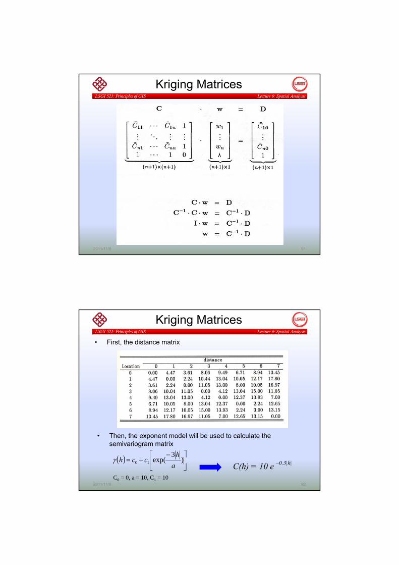
Kriging Matrices

2011/11/8 91

To solve for the weights, we multiply both sides by C-1, the inverse of the left-hand side covariance matrix:

λ


Kriging Matrices

2011/11/8 92

• First, the distance matrix

• Then, the exponent model will be used to calculate the semivariogram matrix

C(h) = 10 e –0.3|h|( ) ⎥⎦

⎤⎢⎣

⎡ −+= )

3exp(10 a

hcchγ

C0 = 0, a = 10, C1 = 10


Results

2011/11/8 95

Kriging weights:

Estimated value for point 0:

λ

How can the interpolation variance be estimated?


• Slope– The slope at a point is the angle

measured from the horizontal to a plane tangent to the surface at that point

– The value of the slope will depend on the direction in which it is measured. Slope is commonly measured in the direction of the coordinate axes e.g. in the X-direction and Y-directions.

– The slope measured in the direction at which it is a maximum is termed the gradient

• Aspect– The angle formed by moving clockwise

from north to the direction of maximum slope

Analysis of Surface

2011/11/8 96

Y SLOPE

NORTH

ASPECT


Shade Slope and Aspect Image

2011/11/8 97


• Hillshading: to calculate the location of shadow and the amount of sun incident on the terrain surface when the sun is in a particular position in the sky

Hillshading

2011/11/8 98

Modelling incoming solar radiation (a–f) representing

morning to evening


Visibility Analysis

2011/11/8 99


Sol 953

An Example in NASA’s Mars Exploration Rover Mission

Sol 1204

Sol 1210

2011/11/8 100


Mapping Products at Duck Bay

2011/11/8 101

Distribution of the measured 3D points DTM interpolated from the 3D points


102

3D Surface of Duck Bay

2011/11/8


103

3D Surface and Slope Maps of Duck Bay

LegendSlope (degree)

0 - 5

5 - 10

10 - 15

15 - 20

20 - 25

25 - 80

2011/11/8


• Further readings– Y. H. Chou, 1997. Exploring Spatial Analysis in Geographic Information Systems,

Onword Press. – Caroline Lafleur, 2011, MATLAB Kriging Toolbox.

(http://globec.whoi.edu/software/kriging/V3/english.html)– ArcGIS Network Analyst

(http://www.esri.com/software/arcgis/extensions/networkanalyst/index.html)

• Summarization of the main ideas presented in this lecture:

• Questions?

Review

2011/11/8 104

Documents

• Dijkstra's Algorithm • Floyd’s Algorithm 521: Principles of GIS Lecture 6: Spatial Analysis • Dijkstra's Algorithm – To find the shortest path from the origin node to the