Embed Size (px)
Citation preview
© Deloitte Consulting, 2004
Loss Reserving Using Policy-Level Data
James Guszcza, FCAS, MAAA Jan Lommele, FCAS, MAAA
Frank ZizzamiaCLRS
Las VegasSeptember, 2004

2
© Deloitte Consulting, 2004
Agenda
Motivations for Reserving at the Policy Level
Outline one possible modeling framework
Sample Results

© Deloitte Consulting, 2004
Motivation
Why do Reserving at the Policy Level?

4
© Deloitte Consulting, 2004
2 Basic Motivations
1. Better reserve estimates for a changing book of business Do triangles “summarize away” important patterns? Could adding predictive variables help?
2. More accurate estimate of reserve variability Summarized data require more sophisticated models
to “recover” heterogeneity. Is a loss triangle a “sufficient statistic” for ultimate
losses & variability?

5
© Deloitte Consulting, 2004
(1) Better Reserve Estimates
Key idea: use predictive variables to supplement loss development patterns
Most reserving approaches analyze summarized loss/claim triangles.
Does not allow the use of covariates to predict ultimate losses (other than time-indicators).
Actuaries use predictive variables to construct rating plans & underwriting models.
Why not loss reserving too?

6
© Deloitte Consulting, 2004
Why Use Predictive Variables?
Suppose a company’s book of business has been deteriorating for the past few years.
This decline might not be reflected in a summarized loss development triangle.
However: The resulting change in distributions of certain predictive variables might allow us to refine our ultimate loss estimates.

7
© Deloitte Consulting, 2004
Examples of Predictive Variables
Claim detail infoType of claimTime between claim and reporting
Policy’s historical loss experience Information about agent who wrote the policy Exposure
Premium, # vehicles, # buildings/employees…
Other specificsPolicy age, Business/policyholder age, credit…..

8
© Deloitte Consulting, 2004
More Data Points
Typical reserving projects use claim data summarized to the year/quarter level.
Probably an artifact of the era of pencil-and-paper statistics.
In certain cases important patterns might be “summarized away”.
In the computer age, why restrict ourselves? More data points less chance of over-
fitting the model.

9
© Deloitte Consulting, 2004
Danger of over-fitting
One well known exampleOverdispersed Poisson GLM fit to loss triangle.Stochastic analog of the chain-ladder55 data points20 parameters estimated
parameters have high standard error.
How do we know the model will generalize well on future development?
Policy-level data: 1000’s of data points

10
© Deloitte Consulting, 2004
Out-of-Sample Testing
Policy-level dataset has 1,000’s of data points
Rather than 55 data points.
Provides more flexibility for various out-of-sample testing strategies.
Use of holdout samplesCross-validation
Uses:Model selectionModel evaluation

11
© Deloitte Consulting, 2004
(2) Reserve Variability
Variability ComponentsProcess riskParameter riskModel specification risk
Predictive error = process + parameter riskBoth quantifiableWhat we will focus on
Reserve variability should also consider model risk.
Harder to quantify

12
© Deloitte Consulting, 2004
Reserve Variability
Can policy-level data give us a more accurate view of reserve variability?
Process risk: we are not summarizing away variability in the data.
Parameter risk: more data points should lead to less estimation error.
Prediction variance: brute force “bootstrapping” easily combines Process & Parameter variance.
Leaves us more time to focus on model risk.

13
© Deloitte Consulting, 2004
Disadvantages
Expensive to gather, prepare claim-detail information.
Still more expensive to combine this with policy-level covariates.
More open-ended universe of modeling options (both good and bad).
Requires more analyst time, computer power, and specialist software.
Less interactive than working in Excel.

© Deloitte Consulting, 2004
Modeling Approach
Sample Model Design

15
© Deloitte Consulting, 2004
Philosophy
Provide an example of how reserving might be done at the policy level
To keep things simple: consider a generalization of the chain-ladder
Just one possible model
Analysis is suggestive rather than definitiveNo consideration of superimposed inflationNo consideration of calendar year effectsModel risk not estimatedetc…

16
© Deloitte Consulting, 2004
Notation
Lj = {L12, L24, …, L120}Losses developed at 12, 24,… monthsDeveloped from policy inception date
PYi = {PY1, PY2, …, PY10 }Policy Years 1, 2, …, 10
{Xk} = covariates used to predict lossesAssumption: covariates are measured at or before
policy inception

17
© Deloitte Consulting, 2004
Model Design
Build 9 successive GLM modelsRegress L24 on L12; L36 on L24 … etc
Each GLM analogous to a link ratio. The Lj Lj+1 model is applied to either
Actual values @ jPredicted values from the Lj-1Lj model
Predict Lj+1 using covariates along with Lj.

18
© Deloitte Consulting, 2004
Model Design
Idea: model each policy’s loss development from period Lj to Lj+1 as a function of a linear combination of several covariates.
Policy-level generalization of the chain-ladder idea. Consider case where there
are no covariates
)...( 111
nnj
j XXfL
L
LinkRatiofL
L
j
j )(1

19
© Deloitte Consulting, 2004
Model Design
Over-dispersed Poisson GLM: Log link function Variance of Lj+1 is proportional to mean
Treat log(Lj) as the offset term Allows us to model rate of loss development
nnj
nn
XXLj
XX
j
j
eL
eL
L
...)log(1
...1
11
11

20
© Deloitte Consulting, 2004
Using Policy-Level Data
Note: we are using policy-level data.Therefore the data contains many zerosPoisson assumption places a point mass at zero
How to handle IBNRInclude dummy variable indicating $0 loss @12 moInteract this indicator with other covariates.
The model will allocate a piece of the IBNR to each policy with $0 loss as of 12 months.

© Deloitte Consulting, 2004
Sample Results

22
© Deloitte Consulting, 2004
Data
Policy Year 1991 – 1st quarter 2000 Workers Comp 1 record per policy, per year Each record has multiple loss evaluations
@ 12, 24, …,120 months
“Losses @ j months” means: j months from the policy inception date.
Losses coded as “missing” where appropriatee.g., PY 1998 losses at 96 months

23
© Deloitte Consulting, 2004
Covariates
Historical LR and claim frequency variables $0 loss @ 12 month indicator Credit Score Log premium Age of Business New/renewal indicator Selected policy year dummy variables
Using a PY dummy variable is analogous to leaving that PY out of a link ratio calculation
Use sparingly

24
© Deloitte Consulting, 2004
Covariates
Interaction terms between covariates and the $0-indicator
Most covariates only used for the 1224 GLM
For other GLMs only use selected PY indicators
These GLMs give very similar results to the chain ladder

25
© Deloitte Consulting, 2004
ResultsChain-LadderPY num_pol prem paid_12 paid_24 paid_36 paid_48 paid_60 paid_72 paid_84 paid_96 paid_108 paid_120 ult res1991 51,854 216,399 9,310 48,224 70,688 81,542 88,219 92,492 95,967 97,841 99,280 100,057 1992 39,821 170,851 26,315 54,071 68,369 75,137 79,427 81,789 83,352 84,783 85,776 - 86,448 672 1993 34,327 156,172 24,789 50,174 61,896 68,498 72,421 74,925 77,151 77,957 - - 79,614 1,657 1994 33,431 153,561 23,137 44,758 55,375 61,249 64,047 65,759 66,682 - - - 69,191 2,509 1995 35,168 148,788 23,468 44,315 53,571 60,133 62,999 64,796 - - - - 68,982 4,186 1996 38,005 140,368 22,989 45,112 54,755 59,477 62,659 - - - - - 69,004 6,346 1997 41,291 134,616 23,936 50,725 62,585 68,432 - - - - - - 79,325 10,892 1998 44,418 134,316 26,761 58,536 69,525 - - - - - - - 88,870 19,346 1999 53,210 166,206 36,452 72,571 - - - - - - - - 112,718 40,147 2000 14,588 46,955 10,266 - - - - - - - - - 32,372 22,106
107,860 Link 2.030 1.215 1.103 1.053 1.034 1.026 1.016 1.013 1.008LDF 3.153 1.553 1.278 1.159 1.101 1.065 1.038 1.021 1.008
Policy-Level Model1991 51,854 216,399 9,310 48,224 70,688 81,542 88,219 92,492 95,967 97,841 99,280 100,057 1992 39,821 170,851 26,315 54,071 68,369 75,137 79,427 81,789 83,352 84,783 85,776 86,440 86,440 664 1993 34,327 156,172 24,789 50,174 61,896 68,498 72,421 74,925 77,151 77,957 78,989 79,572 79,572 1,615 1994 33,431 153,561 23,137 44,758 55,375 61,249 64,047 65,759 66,682 67,750 68,624 69,130 69,130 2,448 1995 35,168 148,788 23,468 44,315 53,571 60,133 62,999 64,796 66,176 67,210 68,076 68,578 68,578 3,782 1996 38,005 140,368 22,989 45,112 54,755 59,477 62,659 64,551 65,894 66,923 67,785 68,285 68,285 5,626 1997 41,291 134,616 23,936 50,725 62,585 68,432 72,034 74,167 75,709 76,891 77,882 78,457 78,457 10,024 1998 44,418 134,316 26,761 58,536 69,525 76,672 80,667 83,055 84,782 86,106 87,216 87,860 87,860 18,335 1999 53,210 166,206 36,452 72,571 88,071 97,073 102,130 105,154 107,341 109,017 110,422 111,237 111,237 38,665 2000 14,588 46,955 10,266 21,114 25,653 28,275 29,749 30,629 31,266 31,755 32,164 32,401 32,401 22,135
103,296

26
© Deloitte Consulting, 2004
Comments
Policy-Level model produces results very close to chain-ladder.
is a proper generalization of the chain-ladder
The model covariates are all statistically significant, have parameters of correct sign.
In this case, the covariates seem to have little influence on the predictions.
Might play more of a role in a book where quality of business changes over time.

© Deloitte Consulting, 2004
Model Evaluation
Treat Recent Diagonals as Holdout
10-fold Cross-Validation

28
© Deloitte Consulting, 2004
Test Model by Holding Out Most Recent 2 Calendar Years
ActualPY num_pol prem paid_12 paid_24 paid_36 paid_48 paid_60 paid_72 paid_84 paid_96 paid_108 paid_1201991 51,854 216,399 9,310 48,224 70,688 81,542 88,219 92,492 95,967 97,841 99,280 100,057 1992 39,821 170,851 26,315 54,071 68,369 75,137 79,427 81,789 83,352 84,783 85,776 - 1993 34,327 156,172 24,789 50,174 61,896 68,498 72,421 74,925 77,151 77,957 - - 1994 33,431 153,561 23,137 44,758 55,375 61,249 64,047 65,759 66,682 - - - 1995 35,168 148,788 23,468 44,315 53,571 60,133 62,999 64,796 - - - - 1996 38,005 140,368 22,989 45,112 54,755 59,477 62,659 - - - - - 1997 41,291 134,616 23,936 50,725 62,585 68,432 - - - - - - 1998 44,418 134,316 26,761 58,536 69,525 - - - - - - - 1999 53,210 166,206 36,452 72,571 - - - - - - - - 2000 14,588 46,955 10,266 - - - - - - - - -
Predict CY 1999 & 20001991 51,854 216,399 9,310 48,224 70,688 81,542 88,219 92,492 95,967 97,841 99,280 100,057 1992 39,821 170,851 26,315 54,071 68,369 75,137 79,427 81,789 83,352 84,971 86,179 86,815 1993 34,327 156,172 24,789 50,174 61,896 68,498 72,421 74,925 76,355 77,809 78,916 79,498 1994 33,431 153,561 23,137 44,758 55,375 61,249 64,047 66,101 67,339 68,621 69,597 70,111 1995 35,168 148,788 23,468 44,315 53,571 60,133 63,373 65,378 66,602 67,870 68,836 69,344 1996 38,005 140,368 22,989 45,112 54,755 60,864 64,108 66,137 67,376 68,658 69,635 70,149 1997 41,291 134,616 23,936 50,725 62,126 69,017 72,696 74,997 76,401 77,856 78,963 79,545 1998 44,418 134,316 26,761 54,215 66,071 73,400 77,313 79,759 81,253 82,800 83,978 84,597 1999 53,210 166,206 36,452 73,695 89,770 99,728 105,045 108,369 110,398 112,500 114,100 114,942 2000 14,588 46,955 10,266 20,833 25,412 28,231 29,736 30,677 31,251 31,846 32,299 32,537
CY1999 error -7.4% -0.7% 2.3% 0.6% 0.5% -1.0% 0.2% 0.5%CY2000 error 1.5% -5.0% 0.9% 2.3% 0.9% 1.0% -0.2%

29
© Deloitte Consulting, 2004
Cross-Validation Methodology
Randomly break data into 10 pieces Fit the 9 GLM models on pieces 1…9
Apply it to Piece 10Therefore Piece 10 is treated as out-of-sample data
Now use pieces 1…8,10 to fit the nine models; apply to piece 9
Cycle through 8 other cases

30
© Deloitte Consulting, 2004
Cross-Validation Methodology
Fit 90 GLMs in all10 cross-validation iterationsEach involving 9 GLMs
Each of the 10 “predicted” pieces will be a 10x10 matrix consisting entirely of out-of-sample predicted values
Can compare actuals to predicteds on upper half of the matrix
Each cell of the triangle is treated as out-of-sample data

31
© Deloitte Consulting, 2004
Cross-Validation Results
ActualPY paid_12 paid_24 paid_36 paid_48 paid_60 paid_72 paid_84 paid_96 paid_108 paid_1201991 9,310 48,224 70,688 81,542 88,219 92,492 95,967 97,841 99,280 100,057 1992 26,315 54,071 68,369 75,137 79,427 81,789 83,352 84,783 85,776 - 1993 24,789 50,174 61,896 68,498 72,421 74,925 77,151 77,957 - - 1994 23,137 44,758 55,375 61,249 64,047 65,759 66,682 - - - 1995 23,468 44,315 53,571 60,133 62,999 64,796 - - - - 1996 22,989 45,112 54,755 59,477 62,659 - - - - - 1997 23,936 50,725 62,585 68,432 - - - - - - 1998 26,761 58,536 69,525 - - - - - - - 1999 36,452 72,571 - - - - - - - - 2000 10,266 - - - - - - - - -
Predicted1991 9,310 48,445 70,884 81,792 88,506 92,746 96,186 97,687 98,946 99,674 0% 0% 0% 0% 0% 0% 0% 0% 0% 0%1992 26,315 54,089 68,418 75,154 79,072 81,412 83,103 84,399 85,487 86,117 0% 0% 0% 0% 0% 0% 0% 0% 0%1993 24,789 50,209 61,157 67,413 70,921 73,023 74,537 75,699 76,676 77,243 0% 0% -1% -2% -2% -3% -3% -3%1994 23,137 44,796 54,618 60,194 63,326 65,198 66,559 67,601 68,475 68,977 0% 0% -1% -2% -1% -1% 0%1995 23,468 44,353 54,064 59,572 62,682 64,534 65,879 66,913 67,775 68,272 0% 0% 1% -1% -1% 0%1996 22,989 47,767 58,181 64,126 67,464 69,463 70,911 72,016 72,940 73,477 0% 6% 6% 8% 8%1997 23,936 49,471 60,164 66,295 69,758 71,820 73,318 74,467 75,428 75,981 0% -2% -4% -3%1998 26,761 55,002 66,781 73,601 77,432 79,725 81,385 82,658 83,724 84,340 0% -6% -4%1999 36,452 74,740 90,704 99,963 105,172 108,285 110,541 112,272 113,720 114,556 0% 3%2000 10,266 21,100 25,631 28,256 29,727 30,609 31,243 31,734 32,145 32,383 0%

© Deloitte Consulting, 2004
Reserve Variability
Using the Bootstrap to estimate the probability distribution of one’s
outstanding loss estimate

33
© Deloitte Consulting, 2004
The Bootstrap
The Statistician Brad Efron proposed a very simple and clever idea for mechanically estimating confidence intervals: The Bootstrap.
The idea is to take multiple resamples of your original dataset.
Compute the statistic of interest on each resample
you thereby estimate the distribution of this statistic!

34
© Deloitte Consulting, 2004
Motivating Example
Suppose we take 1000 draws from the normal(500,100) distribution
Sample mean ≈ 500 what we expect a point estimate of the
“true” mean
From theory we know that:
98.96STD
499.23MEAN
836.87MAX
181.15MIN
1000.00N
valuestatistic
98.96STD
499.23MEAN
836.87MAX
181.15MIN
1000.00N
valuestatistic
16.31000
100/).(. NXds
35
© Deloitte Consulting, 2004
Sampling with Replacement
Draw a data point at random from the data set. Then throw it back in
Draw a second data point. Then throw it back in…
Keep going until we’ve got 1000 data points. You might call this a “pseudo” data set.
This is not merely re-sorting the data. Some of the original data points will appear more than
once; others won’t appear at all.

36
© Deloitte Consulting, 2004
Sampling with Replacement
In fact, there is a chance of
(1-1/1000)1000 ≈ 1/e ≈ .368
that any one of the original data points won’t appear at all if we sample with replacement 1000 times.
any data point is included with Prob ≈ .632
Intuitively, we treat the original sample as the “true population in the sky”.
Each resample simulates the process of taking a sample from the “true” distribution.

37
© Deloitte Consulting, 2004
Resampling
Sample with replacement 1000 data points from the original dataset S Call this S*1
Now do this 399 more times! S*1, S*2,…, S*400
Compute X-bar on each of these 400 samples
S*N
...
S*10
S*9
S*8
S*7
S*6
S*5
S*4
S*3
S*2
S*1
S
38
© Deloitte Consulting, 2004
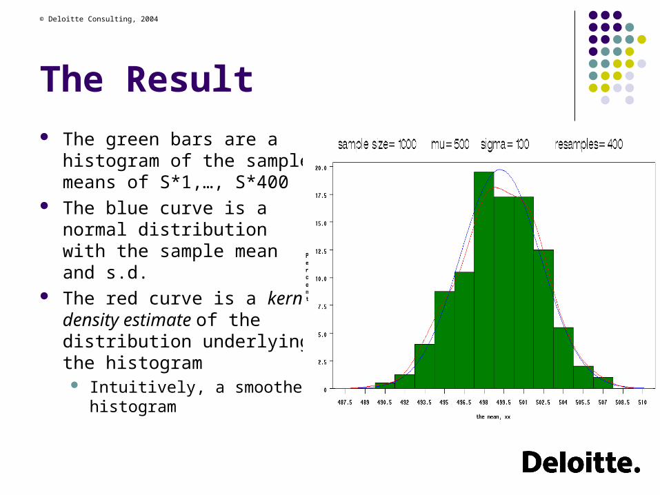
The Result
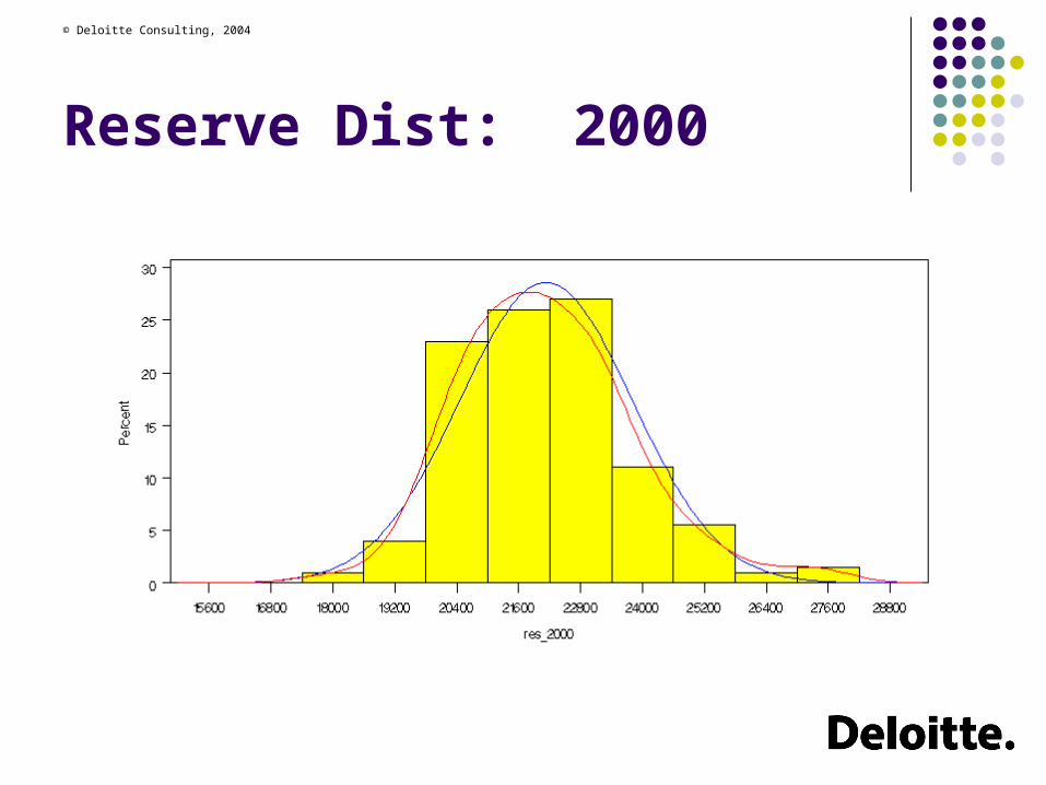
The green bars are a histogram of the sample means of S*1,…, S*400
The blue curve is a normal distribution with the sample mean and s.d.
The red curve is a kernel density estimate of the distribution underlying the histogram Intuitively, a smoothed
histogram

39
© Deloitte Consulting, 2004
The Result
The result is an estimate of the distribution of X-bar.
Notice that it is normal with mean≈500 and s.d.≈3.2
The purely mechanical bootstrapping procedure produces what theory tells us to expect.
Can we use resampling to estimate the distribution of outstanding liabilities?

40
© Deloitte Consulting, 2004
Bootstrapping Reserves
S = our database of policies Sample with replacement all
policies in S Call this S*1
Same size as S Now do this 199 more
times! S*1, S*2,…, S*200
Estimate o/s reserves on each sample
Get a distribution of reserve estimates
S*N
...
S*10
S*9
S*8
S*7
S*6
S*5
S*4
S*3
S*2
S*1
S

41
© Deloitte Consulting, 2004
Bootstrapping Reserves
Compute your favorite reserve estimate on each S*k
These 200 reserve estimates constitute an estimate of the distribution of outstanding losses
Notice that we did this by resampling our original dataset S of policies.
This differs from other analyses which bootstrap the residuals of a model.
Perhaps more theoretically intuitive.But relies on assumption that your model is correct!

42
© Deloitte Consulting, 2004
Bootstrapping Results
Standard Deviation ≈ 5% of total o/s losses 95% confidence interval ≈ (-10%, +10%)
Tighter interval than typically seen in the literature. Result of not summarizing away variability info?
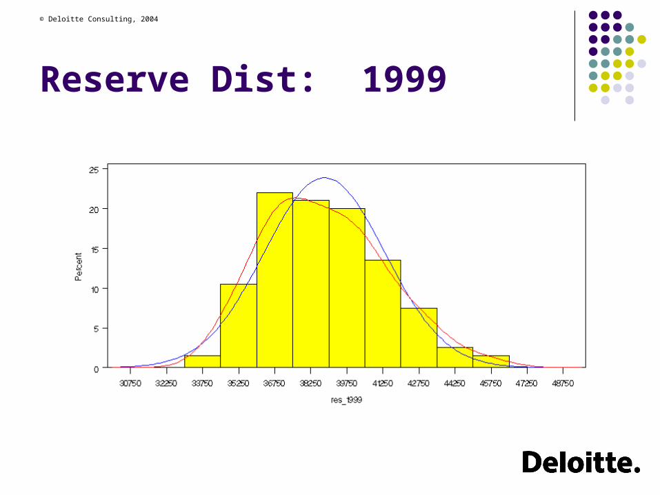
year reserve stdev %1992 651 187 28.8%1993 1,584 274 17.3%1994 2,444 360 14.7%1995 3,747 453 12.1%1996 5,631 503 8.9%1997 9,972 720 7.2%1998 18,273 1,166 6.4%1999 38,820 2,508 6.5%2000 22,128 1,676 7.6%total 103,250 5,304 5.1%

43
© Deloitte Consulting, 2004
Reserve Dist: All Years

44
© Deloitte Consulting, 2004
Reserve Dist: 1992

45
© Deloitte Consulting, 2004
Reserve Dist: 1993

46
© Deloitte Consulting, 2004
Reserve Dist: 1994

47
© Deloitte Consulting, 2004
Reserve Dist: 1995

48
© Deloitte Consulting, 2004
Reserve Dist: 1996

49
© Deloitte Consulting, 2004
Reserve Dist: 1997

50
© Deloitte Consulting, 2004
Reserve Dist: 1998
51
© Deloitte Consulting, 2004
Reserve Dist: 1999
52
© Deloitte Consulting, 2004
Reserve Dist: 2000

53
© Deloitte Consulting, 2004
Interpretation
This result suggests:With 95% confidence, the total o/s losses will be
within +/- 10% of our estimate.Assumes model is correctly specified.
Too good to be true?Yes: doesn’t include model risk!Tighter confidence than often seen in the literature.Bootstrapping a model can be tricky.However: we are using 1000s of data points!We’re not throwing away heterogeneity info.

54
© Deloitte Consulting, 2004
Closing Thoughts
The +/- 10% result is only suggestiveApplies to this specific data set.Bootstrapping methodology can be refined.
Suggestion: using policy-level data can yield tighter confidence intervals
Doesn’t throw away information pertaining to process & parameter risk.
Bootstrapping is conceptually simple.Requires more computer power than brain power!Leaves us more time to focus on model risk.