Copyright Warning & Restrictions

The copyright law of the United States (Title 17, United States Code) governs the making of photocopies or other

reproductions of copyrighted material.

Under certain conditions specified in the law, libraries and archives are authorized to furnish a photocopy or other

reproduction. One of these specified conditions is that the photocopy or reproduction is not to be “used for any

purpose other than private study, scholarship, or research.” If a, user makes a request for, or later uses, a photocopy or reproduction for purposes in excess of “fair use” that user

may be liable for copyright infringement,

This institution reserves the right to refuse to accept a copying order if, in its judgment, fulfillment of the order

would involve violation of copyright law.

Please Note: The author retains the copyright while the New Jersey Institute of Technology reserves the right to

distribute this thesis or dissertation

Printing note: If you do not wish to print this page, then select “Pages from: first page # to: last page #” on the print dialog screen

The Van Houten library has removed some of the personal information and all signatures from the approval page and biographical sketches of theses and dissertations in order to protect the identity of NJIT graduates and faculty.

ABSTRACT

INFORMATION RETRIEVAL AND MININGIN HIGH DIMENSIONAL DATABASES

byXiong Wang

This dissertation is composed of two parts. In the first part, we present a framework

for finding information (more precisely, active patterns) in three dimensional (3D)

graphs. Each node in a graph is an undecomposable or atomic unit and has a label.

Edges are links between the atomic units. Patterns are rigid substructures that may

occur in a graph after allowing for an arbitrary number of whole-structure rotations

and translations as well as a small number (specified by the user) of edit operations

in the patterns or in the graph. (When a pattern appears in a graph only after the

graph has been modified, we call that appearance "approximate occurrence.") The

edit operations include relabeling a node, deleting a node and inserting a node. The

proposed method is based on the geometric hashing technique, which hashes node-

triplets of the graphs into a 3D table and compresses the label-triplets in the table.

To demonstrate the utility of our algorithms, we discuss two applications of them in

scientific data mining. First, we apply the method to locating frequently occurring

motifs in two families of proteins pertaining to RNA-directed DNA Polymerase and

Thymidylate Synthase, and use the motifs to classify the proteins. Then we apply

the method to clustering chemical compounds pertaining to aromatic, bicyclicalkanes

and photosynthesis. Experimental results indicate the good performance of our

algorithms and high recall and precision rates for both classification and clustering.

We also extend our algorithms for processing a class of similarity queries in databases

of 3D graphs.

In the second part of the dissertation, we present an index structure, called

MetricMap, that takes a set of objects and a distance metric and then maps those

objects to a k-dimensional pseudo-Euclidean space in such a way that the distances

among objects are approximately preserved. Our approach employs sampling and

the calculation of eigenvalues and eigenvectors. The index structure is a useful tool

for clustering and visualization in data intensive applications, because it replaces

expensive distance calculations by sum-of-square calculations. This can make

clustering in large databases with expensive distance metrics practical.

We compare the index structure with another data mining index structure,

FastMap, proposed by Faloutsos and Lin, according to two criteria: relative error

and clustering accuracy. For relative error, we show that (i) FastMap gives a lower

relative error than MetricMap for Euclidean distances, (ii) MetricMap gives a

lower relative error than FastMap for non-Euclidean distances (i.e., general distance

metrics), and (iii) combining the two reduces the error yet further. A similar result is

obtained when comparing the accuracy of clustering. These results hold for different

data sizes. The main qualitative conclusion is that these two index structures

capture complementary information about distance metrics and therefore can be

used together to great benefit. The net effect is that multi-day computations can be

done in minutes.

We have implemented the proposed algorithms and the MetricMap index

structure into a toolkit. This toolkit will be useful for data mining, visualization,

and approximate retrieval in scientific, multimedia and high dimensional databases.

INFORMATION RETRIEVAL AND MININGIN HIGH DIMENSIONAL DATABASES

byXiong Wang

A DissertationSubmitted to the Faculty of

New Jersey Institute of Technologyin Partial Fulfillment of the Requirements for the Degree of

Doctor of Philosophy

Department of Computer and Information Science

October 2000

Copyright © 2000 by Xiong Wang

ALL RIGHTS RESERVED

APPROVAL PAGE

INFORMATION RETRIEVAL AND MININGIN HIGH DIMENSIONAL DATABASES

Xiong Wang

Dr. Jason T. L. Wang, Dissertation Advisor DateAssociate Professor of Computer Science, NJIT

Dr. James A. M. McHugh, Committee Member DateProfessor of Computer Science, NJIT

Dr. David Nassimi, Committee Member DateAssociate Professor of Computer Science, NJIT

Dr. Frank Y. Shih, Committee Member DateProfessor of Computer Science, NJIT

Dr. Euthimios Panagos, Committee Member DateMember of Technical Staff, AT&T Labs Research, NJ

BIOGRAPHICAL SKETCH

Author: Xiong Wang

Degree: Doctor of Philosophy

Date: October 2000

Undergraduate and Graduate Education:

• Doctor of Philosophy in Computer Science,New Jersey Institute of Technology, 2000

• Master of Science in Computer Science,Fudan University, Shanghai, China, 1989

• Bachelor of Science in Mathematics,Xiamen University, China, 1982

Major: Computer Science

Presentations and Publications:

Xiong Wang, Jason T.L. Wang, Dennis Shasha, Bruce Shapiro, Isidore Rigoutsos,and Kaizhong Zhang, "Finding Patterns in Three Dimensional Graphs:Algorithms and Applications to Scientific Data Mining", Research Report,Computer and Information Science Department, New Jersey Institute ofTechnology, CIS-99-04. Also submitted to IEEE Transaction on Knowledgeand Data Engineering.

Xiong Wang and Jason T.L. Wang, "Fast Similarity Search in Three-DimensionalStructure Databases", Submitted to The Journal of Chemical Information andComputer Sciences.

Xiong Wang and Jason T.L. Wang, "Implementation and Evaluation of An IndexStructure for Data Clustering", to appear in Knowledge and InformationSystems: An International Journal.

Jason T.L. Wang, Xiong Wang, King-Ip Lin, Dennis Shasha, Bruce A. Shapiro,and Kaizhong Zhang, "Evaluating A Class of Distance-Mapping Algorithms forData Mining and Clustering", Proc. of the Fifth ACM SIGKDD InternationalConference on Knowledge Discovery and Data Mining, pages 307 — 311, August1999, San Diego, California, U.S.A.

iv

Xiong Wang and Jason T. L. Wang, "Fast Similarity Search in Databases of 3DObjects", Proc. of the 10th IEEE International Conference on Tools withArtifical Intelligence, pages 16 — 23, November 1998, Taipei, Taiwan.

Yanling Yang, Kaizhong Zhang, Xiong Wang, Jason T.L. Wang and Dennis Shasha,"An Approximate Oracle for Distance in Metric Spaces" , In M. Farach-Colton,editor, Combinatorial Pattern Matching, pages 104 — 117, Lecture Notes inComputer Science, Springer-Verlag, 1998.

Xiong Wang, Jason T.L. Wang, Dennis Shasha, Bruce Shapiro, Sitaram Dikshitulu,Isidore Rigoutsos and Kaizhong Zhang, "Automated Discovery of Active Motifsin Three Dimensional Molecules" , Proc. of the Third International Conferenceon Knowledge Discovery and Data Mining, pages 89 — 95, August 1997,Newport Beach, California.

Xiong Wang and Jason T.L. Wang, "approximate Substructure Search in aDatabase of 3D Graphs" , Proc. of the Third Joint Conference on Infor-mation Sciences, pages 12 — 15, March 1997, Research Triangle Park, NorthCarolina.

Xiong Wang and Baile Shi, "Query Optimization in a Knowledge Base System" ,Proc. of the Second Far-East Workshop on Future Database Systems, pages327 — 330, April 1992, Kyoto, Japan.

This work is dedicated tomy wife and parents

vi

ACKNOWLEDGMENT

First of all, I would like to thank my advisor Dr. Jason T. L. Wang for his patience,

encouragement and help. He was always there to answer whatever question I had

at any time. I wish also to thank Dr. Dennis Shasha, whose comments have been

so inspiring. Their dedication to the academic career sets an example for me. I

appreciate the cooperation with Dr. Kaizhong Zhang, Dr. Isidore Rigoutsos and Dr.

Bruce Shapiro. Working with them has been so exciting.

I am grateful to Dr. James McHugh, Dr. David Nassimi, Dr. Frank Shih, and

Dr. Euthimios Panagos for their serving in my dissertation committee.

Finally, I thank my wife and my parents, without whose love and support this

accomplishment will not be possible.

vii

TABLE OF CONTENTS

Chapter Page

1 INTRODUCTION 1

2 FINDING PATTERNS IN THREE DIMENSIONAL GRAPHS:ALGORITHMS AND AN APPLICATION TO DATA MINING 4

2.1 Introduction 4

2.2 Related Work 4

2.3 3D Graphs in the Euclidean Space 10

2.3.1 Patterns in 3D Graphs 13

2.4 Pattern-Finding Algorithm 15

2.4.1 Terminology 15

2.4.2 Phase (1) of the Algorithm 16

2.4.3 Phase (2) of the Algorithm 17

2.5 Performance Evaluation 33

2.5.1 Effect of Data-Related Parameters 34

2.5.2 Effect of Algorithm-Related Parameters 36

2.6 Data Mining Applications 41

2.6.1 Classifying Proteins 41

2.6.2 Clustering Compounds 45

2.7 Conclusion 47

3 FAST SIMILARITY SEARCH IN DATABASES OF 3D GRAPHS 49

3.1 Introduction 49

3.1.1 Similarity Search and Related Queries 49

3.2 Preliminaries 50

3.2.1 The Common Edge Table 51

3.2.2 Encoding Node and Label Triplets 52

3.3 Our Approach 52

viii

Chapter Page

3.3.1 Preprocessing Phase 52

3.3.2 On-Line Phase 53

3.3.3 Augmenting Substructure Matches 57

3.3.4 Query Processing Algorithms 60

3.4 Experimental Results 62

4 AN APPROXIMATE ORACLE FOR DISTANCE IN METRIC SPACES 64

4.1 Introduction 64

4.2 Related Work 64

4.3 Mapping Data Objects to a Vector Space 67

4.3.1 Pseudo-Euclidean Space Rk 68

4.3.2 Ψ-Orthogonal Basis {e i} 70

4.3.3 Pseudo-Euclidean Space lin , n < k 72

4.3.4 ø-Orthonormal Basis {ei} 74

4.3.5 Pseudo-Euclidean Space Fr , m < n 76

4.4 Projection of a Target Object 77

4.4.1 Projection of an Embeddable Target 78

4.4.2 Projection of an Unembeddable Target 84

4.5 Experiments and Applications 88

5 AN EXPERIMENTAL EVALUATION OF DISTANCE-EMBEDDINGDATA STRUCTURES 91

5.1 Introduction 91

5.2 Related Work 92

5.3 FastMap and MetricMap: a Brief Comparison 93

5.3.1 The FastMap Algorithm 94

5.3.2 The MetricMap Algorithm 96

5.4 Precision of Embedding 101

5.4.1 Data 101

5.4.2 Experimental Results 102

ix

Chapter Page

5.5 Clustering 110

5.5.1 Data 110

5.5.2 Experimental Results 112

5.6 Discussion 116

5.7 Conclusion 119

6 THE TOOLKIT 121

6.1 Pdiscover 121

6.2 Gsearch 126

6.3 MetricMap 132

6.3.1 The MetricMap system 132

6.3.2 The Clustering Program Average Group Method 137

6.3.3 The Clustering Program CURE 141

6.3.4 The Best Match Search and Range Search Program UsingMetricMap 145

7 SUMMARY OF THE THESIS AND FUTURE WORK 149

7.1 Summary 149

7.2 Future Work 150

REFERENCES 151

LIST OF TABLES

Table Page

2.1 Identifiers, labels and global coordinates of the nodes of the graph in Fig.2.3 12

2.2 The node labels of the graph in Fig. 2.3 and their indices in the array A. 20

2.3 Parameters in the pattern-finding algorithm and their base values usedin the experiments. 33

2.4 Statistics concerning the proteins and motifs found in them 43

2.5 Statistics concerning the chemical compounds and patterns found in them. 46

3.1 Node labels and global coordinates for the target graph in Fig. 3.1 . . . . 55

3.2 Similarity queries and the algorithms to process them 61

5.1 Parameters and base values used in the experiments for evaluating theprecision of embedding. 102

5.2 Parameters and base values used in the experiments for evaluating theaccuracy of clustering Euclidean vectors. 112

LIST OF TABLES

Table Page

2.1 Identifiers, labels and global coordinates of the nodes of the graph in Fig.2.3 12

2.2 The node labels of the graph in Fig. 2.3 and their indices in the array A. 20

2.3 Parameters in the pattern-finding algorithm and their base values usedin the experiments. 33

2.4 Statistics concerning the proteins and motifs found in them 43

2.5 Statistics concerning the chemical compounds and patterns found in them. 46

3.1 Node labels and global coordinates for the target graph in Fig. 3.1 . . . 55

3.2 Similarity queries and the algorithms to process them 61

5.1 Parameters and base values used in the experiments for evaluating theprecision of embedding. 102

5.2 Parameters and base values used in the experiments for evaluating theaccuracy of clustering Euclidean vectors. 112

xi

LIST OF FIGURES

Figure Page

2.1 The reference system and affine coordinates. 6

2.2 The generalized Hough transform. 9

2.3 A data graph G 11

2.4 The substructures of the data graph in Fig. 2 3 12

2.5 (a) The set S of three graphs; (b) the pattern exactly occurring intwo graphs in S; (c) the pattern approximately occurring, within onemutation, in all the three graphs. 14

2.6 Algorithm for finding rigid substructures in a graph. 18

2.7 Calculation of the coordinates of the basis points Pb 1 , Pb2 Pb3 ofSubstructure Frame 0 (SF0) with respect to the local coordinateframe LF[i, j, k]. 21

2.8 The local coordinates, with respect to BF° , of nodes 0, 1, 2, 3, 4 in thesubstructure Str0 of Fig. 2.4(a) 22

2.9 Augmenting two node-triplet matches 28

2.10 A substructure (pattern) P 28

2.11 Running times as a function of the number of graphs. 35

2.12 Recall as a function of the number of graphs. 36

2.13 Number of false matches as a function of the number of graphs. 37

2.14 Effect of Size. 38

2.15 Effect of Mut. 38

2.16 Impact of Scale . 39

2.17 Recall as a function of E . 39

2.18 Precision as a function of E 40

2.19 Number of false matches as a function of Scale. 41

2.20 (a) A 3D protein. (b) The three substructures of the protein in (a). . . . 42

3.1 A target graph Q 54

O f

X11

Figure Page

3.2 The two substructure from the target graph in Fig. 3.1 54

3.3 The matches between the substructures of the target and data graphs . 56

3.4 Augmenting substructure matches 59

3.5 Impact of the decomposition/augmentation processes as a function of thesize of graphs 62

3.6 Performance comparison between our method and the exhaustive searchtechnique 63

4.1 Illustration of the projection method used in FastMap 65

4.2 The mapping a 69

4.3 The Ψ-Orthogonal Basis {e i} and the ø-Orthonormal Basis { 71

4.4 The projection from Rk to Rn 73

4.5 The projection from Rn to Rm. 77

4.6 The projection of a target object 78

4.7 Average absolute errors as a function of the dimension m of the pseudo-Euclidean spaces. 89

4.8 Standard deviations as a function of the dimension m of the pseudo-Euclidean spaces. 89

4.9 Average relative errors as a function of the dimension m of the pseudo-Euclidean spaces. 90

5.1 Illustration of the MetricMap algorithm (k = 2). 98

5.2 Average relative errors of the mappers as a function of the dimensionality

of the target space for synthetic Euclidean data 104

5.3 Effect of dataset size for synthetic Euclidean data 104

5.4 Average relative errors of the mappers as a function of the dimensionalityof vectors for synthetic Euclidean data 105

5.5 Effect of coordinate ranges for synthetic Euclidean data. 105

5.6 Average relative errors of the mappers as a function of the dimensionalityof the target space for synthetic non-Euclidean data. 106

5.7 non-euclidean-datasize-fig 107

5.8 non-euclidean-drange-fig 108

Figure Page

5.9 Average relative errors of the mappers as a function of the dimensionalityof the target space for RNA secondary structures. 108

5.10 Accuracy of MaxMap for synthetic Euclidean data. 110

5.11 Accuracy of AvgMap for synthetic non-Euclidean data. 111

5.12 Mis-clustering rates of the mappers as a function of the dimensionalityof the target space for synthetic Euclidean data 113

5.13 Mis-clustering rates of the mappers as a function of the dimensionalityof the target space for RNA data 114

5.14 Impact of the number of clusters 115

5.15 Impact of the size of clusters 115

5.16 Effect of the dimensionality of vectors in a cluster 116

5.17 Running times of the mappers as a function of the dimensionality of thetarget space for synthetic Euclidean data. 117

5.18 Running times of the mappers as a function of the dimensionality of thetarget space for synthetic non-Euclidean data. 118

xiv

CHAPTER 1

INTRODUCTION

In recent years, much effort has been spent in the study of non-traditional data types,

such as sequences [25, 41, 81, 84, 85], trees [12, 73, 75, 91, 103], graphs [90, 104],

and high dimensional objects. These data types arise frequently in many scientific

domains. For example, in molecular biology, they are used to represent DNA and

protein structures [12, 81, 84, 85]. How to efficiently process these data types poses

a challenging problem to the data management community.

This dissertation focuses on information retrieval, discovery, and clustering in

high dimensional databases and metric spaces. In the first part of the dissertation, we

introduce an approach to approximate pattern discovery in a database of three dimen-

sional graphs (or objects) [96]. Our approach is an extension of the geometric hashing

technique invented by Lamden and Wolfson for tackling computer vision problems

[48, 49, 99]. Given a database D of 3D graphs, an active pattern is a substructure that

occurs in many graphs. For example, in three dimensional molecules these patterns

are called active motifs. Our algorithm tries to discover patterns that approximately

occur in multiple graphs. A pattern is said to occur in a graph approximately if

it matches a substructure of the graph, possibly in the presence of rotation, trans-

lation and node relabel/insert/delete in either the substructure or the pattern. Our

algorithm finds many applications in for example drug design [26] and molecular

biology [58].

Databases in these domains are often large in size. In order to find all interesting

patterns, one needs to consider lots of possible substructures. Thus the efficiency

of the algorithm is critical. Our approach employing geometric hashing is shown

empirically to be very efficient. We then extend the algorithm to process a class

of similarity queries in databases of 3D objects. We applied our query processing

1

2

algorithms to 226 chemical compounds obtained from a drug database maintained

in the National Cancer Institute, and a set of synthetic graphs. The experimental

results showed that our technique is 100 times faster than the exhaustive search

method when the data set has over 600 objects while achieving the same recall.

In the second part of the dissertation, we present an index structure, called

MetricMap, that takes a set of objects and a distance metric and then maps those

objects to a k-dimensional pseudo-Euclidean space in such a way that the distances

among objects are approximately preserved. Our approach employs sampling and

the calculation of eigenvalues and eigenvectors. The index structure is a useful tool

for clustering and visualization in data intensive applications [101]. MetricMap

differs from another data mining index structure, FastMap, proposed by Faloutsos

and Lin, in the algorithm it uses for embedding and the target space it chooses.

FastMap embeds the objects in a Euclidean space, whereas MetricMap embeds

them in a pseudo-Euclidean space [33, 50]. We compare the two index structures

according to two criteria: relative error and clustering accuracy [92, 97]. For relative

error, we show that (i) FastMap gives a lower relative error than MetricMap for

Euclidean distances, (ii) MetricMap gives a lower relative error than FastMap for

non-Euclidean distances (i.e., general distance metrics), and (iii) combining the two

reduces the error yet further. A similar result is obtained when comparing the

accuracy of clustering. These results hold for different data sizes. The main quali-

tative conclusion is that these two index structures capture complementary infor-

mation about distance metrics and therefore can be used together to great benefit.

The net effect is that multi-day computations can be done in minutes.

In Chapter 2, we present the framework for finding patterns in 3D graphs and its

application to the discovery of motifs in proteins and chemical compounds. Chapter

3 extends the algorithm to process a class of similarity queries in databases of 3D

graphs. Chapter 4 describes the MetricMap index structure and its performance in

3

approximating distances for both artificial data and real data. Chapter 5 compares

FastMap with MetricMap, builds some complementary index structures, and

compares the relative performance of these index structures. Chapter 6 describes

the toolkit containing the programs for pattern discovery and similarity retrieval in

3D graphs using the geometric hashing technique as well as the MetricMap index

structure. Chapter 7 concludes the dissertation and discusses future work.

CHAPTER 2

FINDING PATTERNS IN THREE DIMENSIONAL GRAPHS:ALGORITHMS AND AN APPLICATION TO DATA MINING

2.1 Introduction

In this Chapter, we introduce an approach for finding patterns in a database of

3D graphs. Given a database D of 3D graphs, An active pattern is a common

substructure that occurs in more than one graph. For example, in three dimensional

molecules these patterns are called active motifs. Our algorithm tries to discover

patterns that approximately occur in more than one graph. A pattern is said to occur

in a graph approximately if it matches a substructure of the graph approximately

in the presence of rotation, translation and node relabel/insert/delete in either the

substructure or the pattern. This is an extension of the traditional substructure

match in scientific and biochemical databases [66]. Our approach is based on the

geometric hashing technique.

The rest of the chapter is organized as follows. Section 2.2 is a survey of

related work. Section 2.3 formalizes the pattern discovery problem. Section 2.4

presents the theoretical framework of our approach and describes the pattern-finding

algorithm in detail. Section 2.5 evaluates the performance and efficiency of the

pattern-finding algorithm. Section 2.6 discusses the applications of our approach to

classifying proteins and clustering compounds. Section 2.7 concludes the chapter.

2.2 Related Work

There are several groups working on pattern finding (or knowledge discovery) in

molecules and graphs. Conklin et al. [15, 16, 17], for example, represented a

molecular structure as an image, which comprised a set of parts with their 3D

coordinates and a set of relations that were preserved for the image. The authors

used an incremental, divisive approach to discover the "knowledge" from a dataset,

4

5

that is, to build a subsumption hierarchy that summarized and classified the dataset.

The algorithm relied on a measure of similarity among molecular images that was

defined in terms of their largest common subimages.

In [20], Djoko et al. developed a system, called SUBDUE, that utilized the

minimum description length principle to find repeatedly occurring substructures in

a graph. Once a substructure was found, the substructure was used to simplify the

graph by replacing instances of the substructure with a pointer to the discovered

substructure. In [19], Dehaspe et al. used DATALOG to represent compounds

and applied data mining techniques to predicting chemical carcinogenicity. Their

techniques were based on Mannila and Toivonen's algorithm [51] for finding inter-

esting patterns from a class of sentences in a database.

In contrast to the above work, we use the geometric hashing technique to find

approximately common patterns in a set of 3D graphs without prior knowledge of

their structures, positions, or occurrence frequency. The geometric hashing technique

used here originated from the work of Lamdan and Wolfson for model based recog-

nition in computer vision [49]. Several researchers attempted to parallelize the

technique based on various architectures, such as the Hypercube and the Connection

Machine [9, 65, 63]. It was observed that the distribution of the hash table entries

might be skewed. To balance the distribution of the hash function values, delicate

rehash functions were designed [63]. There were also efforts exploring the uncertainty

existing in the geometric hashing algorithms [34, 70].

Recently, Rigoutsos et al. employed geometric hashing and magic vectors for

substructure matching in a database of chemical compounds [66]. The magic vectors

were bonds among atoms; the choice of them was domain dependent and was based

on the type of each individual graph. We extend the work in [66] by providing

a framework for discovering approximately common substructures in a set of 3D

graphs, and applying our techniques to both compounds and proteins. Our approach

6

differs from [66] in that instead of using the magic vectors, we store a coordinate

system in a hash table entry. Furthermore we establish a theory for detecting and

eliminating false matches occurring in the hashing.

Geometric hashing technique was first introduced in late 80's for model based

recognition in computer vision [49]. The key observation behind the technique is as

follows. Suppose D is an object consisting of a set of points in the two dimensional

space R2 . Given any three points P1, P2 and P3 in D that are not collinear, a

coordinate system can be formed using P1 as the origin, P1, P2 as X-axis and PIT, P3

as Y-axis. Any other point P in D has a set of coordinates (x, y) with respect to

this coordinate system (Fig. 2.1(a)). Now suppose under certain rigid rotation or

translation P1 , P2 P3 and P become PL P2 , P3 and P'. P1', P2 and P3 will still be non-

collinear and they can form another coordinate system. Notice that the coordinates

of P' with respect to this new coordinate system is still (x, y) (Fig. 2.1(b)).

Figure 2.1 The reference system and affine coordinates.

Thus these coordinates are geometric invariant. Using the original termi-

nologies, any triplet of points P1, P2 and P3 in D that are non-collinear is called

a reference system RS, and the coordinates of any point P in D with respect to RS

is called the affine coordinates of P w.r.t. RS.

7

The geometric hashing algorithm is composed of two phases. In the prepro-

cessing phase, every ordered triplet of points in D that are not collinear is used as

an RS, and the affine coordinates (x, y) of every other point in D are computed with

respect to the RS. RS is then entered into the hash table at each (x, y) location.

(nFor an object with n points, there are (n — 3) x 3 entries in the hash table.

This process is done for every data object D. In the recognition phase, given a

query object Q, every triplet of points in Q is taken to be a reference system, and

the affine coordinates of all other points in Q are computed with respect to the

reference system to index into the hash table and "vote" for all RS's found there. A

histogram for the RS's is created for each data object. If the number of the votes for

any RS is sufficiently high, that RS and the corresponding data object are collected

as a hypothesis. A verification process is then used to identify the correct answers.

Suppose there is a substructure match between the query object and the data object

and a triplet of points trig in the query object Q matches an RS in a data object.

This RS will get high score in the voting process when triplet trig is chosen as the

reference system during the recognition phase.

Due to the arrangement of hash table, the voting can be done for all data objects

and all RS's in each data object simultaneously. Both phases of the algorithm have

nice features for parallel processing. Algorithms for parallel geometric hashing have

been developed on several different architectures, such as the Hypercube SIMD and

the Connect Machine, e.g. model CM-2, CM-5 [9, 63, 65]. All these algorithms

achieved fine-grain data parallelism.

However, nothing is perfect. The original geometric hashing algorithm has its

drawbacks. Since every triplet of points in the data object is used as a reference

system, the records in the hash table are highly redundant. Furthermore, in the

presence of uncertainty, affine representations are not invariant with respect to the

Cartesian coordinate system. In [34] the authors provided a precise analysis of

8

affine point matching, obtaining an expression for the range of affine-invariant values

consistent with bounded uncertainty. This analysis revealed that the range of affine-

invariant values depends on the original positions of the points. The effect of this

phenomenon is twofold. If it happened in the preprocessing phase when the data

objects were hashed, it would degrade the performance rapidly [34]. Intuitively, due

to uncertainty, the error causes the point entries in the hash table to blur into regions,

making the table denser and increasing the chances that a random point (i.e. a point

does not really belong to any data objects) will appear to be a hypothesis for a match

[70]. One the other hand, if it happened in the recognition phase when the query

object was processed, it would cause both false positive and false negative votes. In

[70] the author analyzed the effect of this phenomenon in the presence of Gaussian

noise.

In [38] the authors discussed the problem of self-affine shapes. A self-affine

shape consists smaller, affine copies of itself or its parts. When geometric hashing

is applied to scenes with lots of self-affine shapes, there is a large proportion

of four-point combinations that produce the same affine-invariant coordinates,

yielding severe spikes in the histogram, which may cause the geometric hashing

method to malfunction [38]. The authors then introduced an alternative approach

called similarity hashing. Like geometric hashing, similarity hashing operates on

combinations of four points. Each group of four points A, B, CandD forms two

line segments AB and CD. The two line segments AB, CD are related by two

parameters: scale and orientation. Assume I IABII > ||CD|| I, the scale s : 0 < s <1

is the ratio of the lengths of the two line segments

The orientation 0 : < 0 < 2is given by the minimum angle that AB rotates to

become parallel to CD. Their experiments demonstrated the ability of this approach

9

at detecting morphological self-similarity, and producing the parameters of the self-

similarity transformation, which helped in the process of fractal image compression.

Figure 2.2 The generalized Hough transform.

It is interesting to compare the geometric hashing techniques with the gener-

alized Hough transform [6, 39]. The generalized Hough transform is also composed

of two phases. We describe here the Hough transform applying to a set of curves.

Given are a set of data curves and a query curve, our goal is to find those data

curves that best match the query curve. In the preprocessing phase, a data curve is

processed as follows (Fig. 2.2).

1. Arbitrarily choose a reference point Po;

2. for each point P on the curve do the following:

(a) calculate the angle 0(P) tangent at P,

(b) store the vector P, P0 at location 0(P) of a hash table.

In the recognition phase, for each point P on the query curve, the angle tangent

at P is used as index to access the hash table. Every reference point P0 at that

location gets one vote. A histogram for the reference point is created for each data

curve, and then analyzed to find matches.

10

Both the geometric hashing technique and the generalized Hough transform

technique use similar object representation schemes and both of them utilize a look

up table to improve the performance.

Comparing with the original geometric hashing technique, our approach

reduces redundancy significantly and is more adjustable to noise. When dealing

with approximate substructure matching, our approach is also more flexible than

both the original geometric hashing technique and the generalized Hough transform

technique.

2.3 3D Graphs in the Euclidean Space

Three dimensional (3D) graphs occur frequently in scientific disciplines. In chemistry,

for example, chemical compounds are 3D graphs [66]. In biology, the tertiary

structures of proteins are also 3D graphs [16, 27]. Each node of such graphs is

an undecomposable or atomic unit and has a 3D coordinate.' Each node has a label,

which is not necessarily unique in a graph. Node labels are chosen from a domain-

dependent alphabet E. In chemical compounds, for example, the alphabet includes

the names of all atoms. A node can be identified by a unique, user-assigned number

in the graph. Edges in the graph are links between the atomic units. We consider

in the chapter the graphs to be connected [53]; otherwise we focus on the connected

components of the graphs.

A graph can be divided into one or more rigid substructures. A rigid

substructure is a subgraph in which there are no internal rotations; that is, the

relative positions of nodes in the substructure are fixed. 2 The precise definition of

1 More precisely, the 3D coordinate indicates the location of the center of the atomicunit.

2 Note that the rigid substructure as a whole can be rotated (we refer to this as a"whole-structure" rotation or simply a rotation when the context is clear). That is to say,the relative position of a node in the substructure and a node outside the substructure canbe changed under the rotation.

11

a "substructure" is application dependent. For example, in chemical compounds,

a ring is a rigid substructure. Thus if we consider a chemical compound as a 3D

graph in which each atom is a node and each bond is an edge, a block [53] of the

graph could be a rigid substructure; two rigid substructures may be connected by

an edge and they may be rotatable with respect to each other around the edge. On

the other hand, in a protein that itself as a whole is a rigid structure, a residue

or a combination of multiple residues as illustrated in Section 2.4 could be a rigid

substructure.

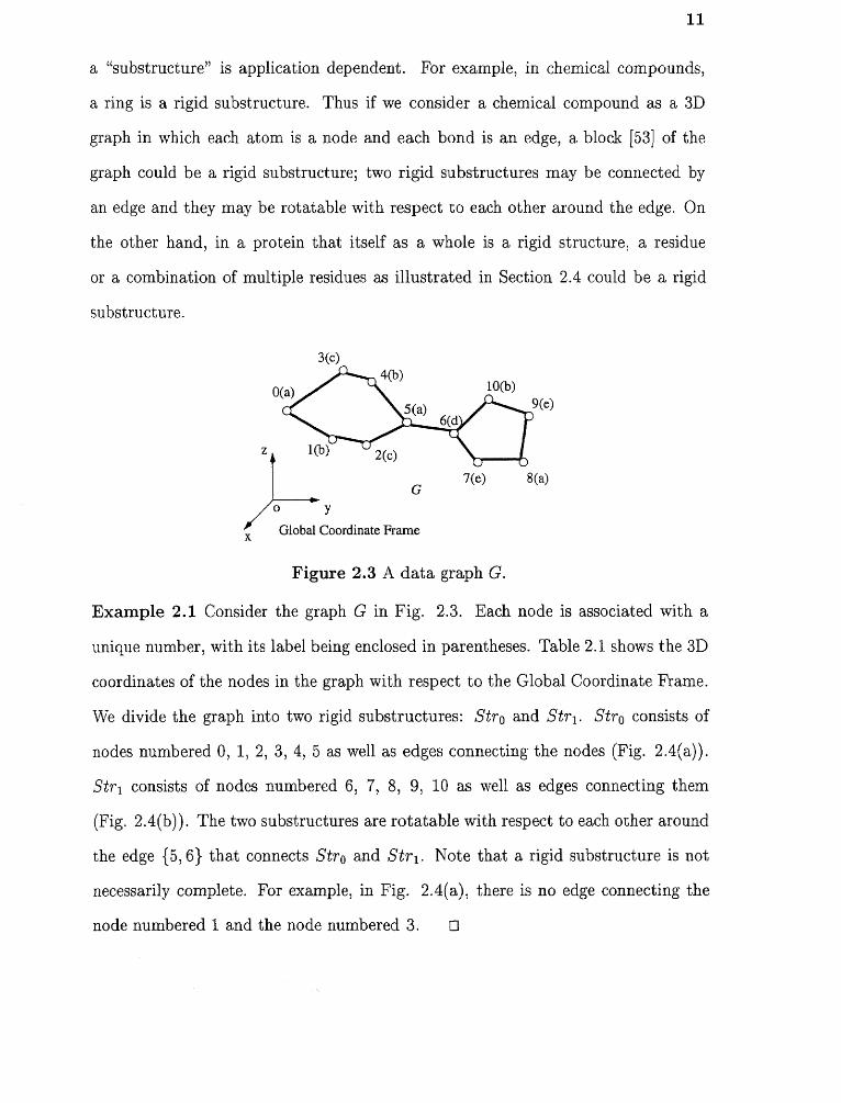
Figure 2.3 A data graph G.

Example 2.1 Consider the graph G in Fig. 2.3. Each node is associated with a

unique number, with its label being enclosed in parentheses. Table 2.1 shows the 3D

coordinates of the nodes in the graph with respect to the Global Coordinate Frame.

We divide the graph into two rigid substructures: Str0 and Str 1 . Stro consists of

nodes numbered 0, 1, 2, 3, 4, 5 as well as edges connecting the nodes (Fig. 2.4(a)).

Str 1 consists of nodes numbered 6, 7, 8, 9, 10 as well as edges connecting them

(Fig. 2.4(b)). The two substructures are rotatable with respect to each other around

the edge {5, 6} that connects Str0 and Str 1 . Note that a rigid substructure is not

necessarily complete. For example, in Fig. 2.4(a), there is no edge connecting the

node numbered 1 and the node numbered 3. ❑

12

Figure 2.4 The substructures of the data graph in Fig. 2.3

Table 2.1 Identifiers, labels and global coordinates of the nodes of the graph in Fig.2.3

Node identifier Node label Node coordinates

0 a (1.0178, 1.0048, 2.5101)1 b (1.2021, 2.0410, 2.0020)2 c (1.3960, 2.9864, 2.0006)3 c (0.7126, 2.0490, 3.1921)4 b (0.7610, 2.7125, 3.0124)5 a (1.0097, 3.6478, 2.2660)6 d (1.1329, 4.5002, 2.2024)7 e (1.5309, 5.2026, 1.7191)8 a (1.4529, 6.1015, 1.5712)9 e (1.0356, 6.0030, 2.2820)

10 b (0.7359, 5.0571, 2.6857)

We attach a local coordinate frame SF° (SF1 , respectively) to substructure

Str0 (Str i , respectively). For instance, let us focus on the substructure Str 0 in

Fig. 2.4(a). We attach a local coordinate frame to Str 0 whose origin is the node

numbered 0. This local coordinate frame is represented by three basis points Pb„

Pb2 and Pb3 , with coordinates Pb1 (x0 Yo, zo), Pb2 (x0 ± 1, Y0, zo) and Pb3 (x0, Y0 -+-1 , z0 ),

respectively. The origin is Pk and the three basis vectors are f)-b1,b2 , Vb1,b3, and

x 17b1 , b3 . Here, frbi ,b2 represents the vector starting at point Pb1 and ending at

point Pb2.yb ,, b2 stands for the cross product of the two corresponding vectors.

We refer to this coordinate frame as Substructure Frame 0, or SF0 . Note that, the

13

basis vectors of SF° are orthonormal. That is, the length of each vector is 1 and the

angle between any two basis vectors has 90 degrees. Also note that, for any node

numbered i in the substructure Str 0 with global coordinate .Pi (x i , yi , zi ), we can find

a local coordinate of the node i with respect to SF0 , denoted Pi, where

2.3.1 Patterns in 3D Graphs

We consider a pattern to be a rigid substructure that may occur in a graph after

allowing for an arbitrary number of rotations and translations as well as a small

number (specified by the user) of edit operations in the pattern or in the graph.

There are three types of edit operations: relabeling a node, deleting a node and

inserting a node. Relabeling a node v means to change the label of v to any valid

label that differs from its original label. Deleting a node v from a graph means to

remove the corresponding atomic unit from the 3D Euclidean space and make the

edges touching v connect with one of its neighbors v'. (This amounts to contraction

of the edge between v and v' [29].) Inserting a node v into a graph means to add

the corresponding atomic unit to the 3D Euclidean space and make a node v' and

a subset of its neighbors become the neighbors of v. 3 Graph G matches graph G'

with n mutations if by applying an arbitrary number of rotations and translations

as well as n node insert, delete or relabeling operations, one can transform G to G'.

A substructure P approximately occurs in a graph G (or G approximately contains

P) within n mutations if P matches some subgraph of G with n mutations or fewer

where n is chosen by the user.

3 Note that when a node v is inserted or deleted, the nodes surrounding v do not move,i.e., their coordinates remain the same. The three edit operations are extensions of the editoperations on sequences; they arise naturally in graph editing [29] and molecule evolution[69]. As shown in Section 2.4, based on these edit operations, our algorithm finds usefulpatterns that can be used to classify and cluster 3D molecules effectively.

14

Example 2.2 Consider the set S of three graphs in Fig. 2.5(a). Suppose only

exactly coinciding substructures (without mutations) occurring in at least two

graphs and having size greater than 3 are considered as "patterns." Then S contains

one pattern shown in Fig. 2.5(b). If substructures having size greater than 4 and

approximately occurring in all the three graphs within one mutation (i.e. one node

delete, insert or relabeling is allowed in matching a substructure with a graph) are

considered as "patterns," then S contains one pattern shown in Fig. 2.5(c).

Figure 2.5 (a) The set S of three graphs; (b) the pattern exactly occurring in twographs in S; (c) the pattern approximately occurring, within one mutation, in allthe three graphs.

Our strategy to find the patterns in a set of 3D graphs is to decompose the

graphs into rigid substructures and then use the geometric hashing technique [49] to

store the substructures in a disk-based table. We then evaluate the substructures in

the hash table to find frequently occurring ones.

15

In [96], we applied the approach to the discovery of patterns in chemical

compounds under a restricted set of edit operations including node insert and node

delete, and tested the quality of the patterns by using them to classify the compounds.

Here we extend the work in [96] by (i) considering more general edit operations

including node insert, delete and relabeling; (ii) presenting the theoretical foundation

and evaluating the performance and efficiency of our pattern-finding algorithm; (iii)

applying the discovered patterns to classifying 3D proteins, which are much larger

and more complicated in topology than chemical compounds; and (iv) presenting a

technique to cluster 3D graphs based on the patterns occurring in them [98]. Classi-

fication and clustering are two important data mining operations in general and

scientific disciplines [2, 3, 36, 86, 87, 105]; here we show experimentally that our

techniques are useful for the scientific data mining applications.

2.4 Pattern-Finding Algorithm2.4.1 Terminology

Let S be a set of 3D graphs. The occurrence number of a pattern P is the number of

graphs in S that approximately contain P within the allowed number of mutations.

Formally, the occurrence number of a pattern P (or the activity of P) with respect to

mutation d and set 5, denoted occurrence_n4(P), is k if there are k graphs in S that

contain P within d mutations. For example, consider Fig. 2.5 again. Let S contain

the three graphs in Fig. 2.5(a). Then occurrence_no°s (Pi ) = 2; occurrence_no ls (P2 )

= 3.

Given a set S of 3D graphs, our algorithm finds all the patterns P where P

approximately occurs in at least Occur graphs in S within the allowed number of

mutations Mut and 1P1 > Size, where IPt represents the size, i.e., the number of

nodes, of the pattern P. (Mut, Occur and Size are user-specified parameters.) One

can use the patterns in several ways. For example, natural scientists may evaluate

16

whether the patterns are in fact the active sites; computer scientists may use the

patterns to classify or cluster molecules as demonstrated in Section 2.4.

Our algorithm proceeds in two phases to search for the patterns: (1) find

candidate patterns from the graphs in S; and (2) evaluate the activity of the

candidate patterns to determine which of them satisfy the user-specified requirements.

We describe each phase in turn below.

2.4.2 Phase (1) of the Algorithm

In phase (1) of the algorithm, we decompose the graphs into rigid substructures.

Dividing a graph into substructures is necessary for two reasons. First, in dealing

with some molecules such as chemical compounds in which there may exist two

substructures that are rotatable with respect to each other, any graph containing the

two substructures is not rigid. As a result, we decompose the graph into substructures

having no rotatable components and consider the substructures separately. Second,

our algorithm hashes node-triplets into a 3D table. When a graph as a whole is

too large, as in the case of proteins, considering all combinations of three nodes

in the graph may become prohibitive. Consequently, decomposing the graph into

substructures and hashing node-triplets of the substructures can increase efficiency.

For example, consider a graph of 20 nodes. There are ( 230 )

— 1140 node-triplets.

On the other hand, if we decompose the graph into five substructures, each having

four nodes, then there are only 5x ( 43 = 20 node-triplets.

There are several alternative ways to decompose 3D graphs into rigid sub-

structures, depending on the application at hand and the nature of the graphs.

The substructures may partition a graph or may overlap with one another. For

example, to find patterns in a chemical compound, one can use a modified depth-first

search algorithm for finding blocks to decompose the compound into substructures

as described in [53, 96]. In this case, the substructures partition the compound.

17

Two substructures may be connected by one bond (edge); they may be rotatable

with respect to each other around the bond (cf. Example 2.1). On the other hand,

for a protein that itself forms a single rigid structure, one can decompose it into

substructures of fixed size according to some order as illustrated in Section 2.4 or

consider each residue as a rigid substructure. In these cases, two substructures may

overlap or may be connected by multiple edges.

For the purposes of exposition, we describe our pattern-finding algorithm based

on a partitioning strategy. Our approach assumes a notion of atomic unit which is

the lowest level of description in the case of interest. Intuitively, atomic units are the

fundamental building blocks, e.g. atoms in a molecule. Edges arise as bonds between

atomic units. We break a graph into maximal size rigid substructures (recall that

a rigid substructure is a subgraph in which there are no internal rotations; that is,

the relative positions of nodes in the substructure are fixed). We use an approach

similar to [53] that employs a depth-first search algorithm, referred to as DFB, to

find blocks in graphs. Each block is a rigid substructure. We merge two rigid

substructures B 1 and B2 if they are not rotatable with respect to each other; that is,

the relative position of a node n 1 E B 1 and a node n2 E B2 is fixed. The algorithm

maintains a stack, denoted ST K, which keeps the rigid substructures being merged.

Fig. 2.6 shows the algorithm, which outputs a set of rigid substructures of a graph

G. We then throw away the substructures P where IP! < Size. The remaining

substructures constitute the candidate patterns generated from G. This pattern-

generation algorithm runs in time linearly proportional to the number of edges in

G.

2.4.3 Phase (2) of the Algorithm

Phase (2) of our pattern-finding algorithm consists of two subphases. In subphase

A of phase (2), we hash the candidate patterns generated from the graphs in phase

18

Procedure Find_Rigid_SubstructuresInput: Graph G.Output: A set of maximal size rigid substructures generated from G.

ST K := 0;while G is not empty do

beginlocate the next block B 1 in G using the DFB algorithm;delete B 1 from G; let the top entry of STK be B2if (STK is empty) or (B 1 and B2 are not rotatable w.r.t. each other) then

push the nodes of B 1 into STK;else begin

pop out all nodes in STK,merge them and output the resulting substructure;push the nodes of B 1 into STK;

end;end;

pop out all nodes in STK, merge them and output the resulting substructure;

Figure 2.6 Algorithm for finding rigid substructures in a graph.

19

(1) into a 3D table fl. In subphase B, we rehash each candidate pattern into N and

evaluate its activity (recall that the activity is the number of approximate occur-

rences).

In processing a rigid substructure (pattern) of a 3D graph, we choose all three-

node combinations, referred to as node-triplets, in the substructure and hash the

node-triplets. We hash three-node combinations, because to fix a rigid substructure

in the 3D Euclidean space one needs at least three nodes from the substructure and

three nodes are sufficient provided they are not collinear. Notice that the proper

order of choosing the nodes i, j, k in a triplet is significant. We determine the order

of the three nodes by considering the triangle formed by them. The first node chosen

always opposes the longest edge of the triangle and the third node chosen opposes the

shortest edge. Thus, the order is unique if the triangle is not isosceles or equilateral,

which usually holds when the coordinates are floating point numbers. In other cases,

we store all configurations obeying the longest-shortest rule described above.

The labels of the nodes in a triplet form a label-triplet, which is encoded as

follows. Suppose the three nodes chosen are v 1 , v2 , v3 , in that order. We maintain all

node labels in the alphabet E in an array A. The code for the labels is an unsigned

long integer, defined as ((L 1 x Prime + L 2) x Prime) + L3, where Prime > lE1

is a prime number, L1, L2 and L3 are the indices for the node labels of v 1 , v2 and

v3 , respectively, in the array A. Thus the code of a label-triplet is unique. This

simple encoding scheme reduces three label comparisons into one integer comparison.

Example 2.3 Consider again the graph G in Fig. 2.3. Suppose the node labels

are stored in the array A as shown in Table 2.2. Suppose Prime is 1,009. Then,

for example, for the three nodes numbered 2, 0 and 1 in Fig. 2.3, the code for the

corresponding label-triplet is ((2 x 1, 009 + 0) x 1, 009) + 1 2,036,163. ❑

20

Table 2.2 The node labels of the graph in Fig. 2.3 and their indices in the array A.

index 0 1 2label a b c d e

2.4.3.1 Subphase A of Phase (2) In this subphase, we hash the candidate

patterns generated in phase (1) of the pattern-finding algorithm into a 3D table. For

the purposes of exposition, consider the example substructure Str0 in Fig. 2.4(a),

which is assumed to be a candidate pattern. We choose any three nodes in Str o

and calculate their 3D hash function values as follows. Suppose the chosen nodes

are numbered i, j, k and have global coordinates Pi (xi, yi, Pi (xi , yi , zi) and

respectively. Let 1 1 , /2 , l 3 be three integers where

Here Scale = 10^p is a multiplier. Intuitively we round to the nearest ptn position

following the decimal point (here p is the last accurate position) and then multiply

the numbers by 10P. The reason for using the multiplier is that we want some digits

following the decimal point to contribute to the distribution of the hash function

values. We ignore the digits after the position p because they are inaccurate. (The

multiplier is a parameter whose value is determined in experiments and is adjustable

for different data.) Let

Prime ' , Prime2 and Prime3 are three prime numbers and Nrow is the cardinality

of the hash table in each dimension. We use three different prime numbers in the

21

hope that the distribution of the hash function values is not skewed even if pairs of

/ 1 , /2 , /3 are correlated. The node-triplet [i, j, k] is hashed to the 3D bin with the

address h[c/ 1 ][d2 ][c/3]. Intuitively we use the squares of the lengths of the three edges

connecting the three chosen nodes to determine the hash bin address. Stored in that

bin are the graph identification number, the substructure identification number, and

the label-triplet code. In addition, we store the coordinates of the basis points Pb1,

Pb2,Pb3of Substructure Frame 0(SF0)with respect to the three chosen nodes.

Specifically, suppose the chosen nodes i, j, k are not collinear. We can construct

another local coordinate frame, denoted LF[i, j, k], using U ,j, jk and ,j x Vi,k as

basis vectors. The coordinates of Pb1, Pb2 , Pb3 with respect to the local coordinate

frame L F [i, j, k], denoted SF0 [i, j, k] , form a 3 x 3 matrix, which is calculated as

follows (see Pip._ 2.71:

Figure 2.7 Calculation of the coordinates of the basis points Pb1, Pb2, Pb3 ofSubstructure Frame 0 (SF0 ) with respect to the local coordinate frame LF[i, j, k].

22

Thus suppose the graph in Fig. 2.3 has identification number 12. The hash bin

entry for the three chosen nodes i, j, k is (12, 0, Lcode, S F0 [i, j, k]), where Lcode is

the label-triplet code. Since there are 6 nodes in the substructure Str o , we have

( 36 )= 20 node-triplets generated from the substructure and therefore 20 entries

in the hash table for the substructure.

Example 2.4 Consider Table 2.1 again. The basis points of SF° of Fig. 2.4(a) have

global coordinates

Fig. 2.8 shows the local coordinates, with respect to SF0 , of the nodes numbered 0,

1, 2, 3 and 4 in substructure Str o of Fig. 2.4(a).

Figure 2.8 The local coordinates, with respect to SF0 , of nodes 0, 1, 2, 3, 4 in thesubstructure Stro of Fig. 2.4(a).

Now, suppose Scale, Prime1, Prime2 , Prime 3 are 10, 1,009, 1,033 and 1,051 respec-

tively, and Nrow is 31. Thus, for example, for the nodes numbered 1, 2 and 3, the

hash bin address is h[25][12][21] and

23

As another example, for the nodes numbered 1, 4 and 2, the hash bin address is

h [24][0][9] and

Similarly, for the substructure Str1 , we attach a local coordinate frame SF 1 to the

node numbered 6 as shown in Fig. 2.4(b). There are 10 hash table entries for Str 1 ,

each having the form (12, 1, Lcode, S F1[1, m, n]) where 1, m, n are any three nodes in

Str 1. ❑

Recall that we choose the three nodes i, j, k based on the triangle formed

by them—the first node chosen always opposes the longest edge of the triangle and

the third node chosen opposes the shortest edge. Without loss of generality, let us

assume that the nodes i, j, k are chosen in that order. Thus, Vi, j has the shortest

length, 174 is the second shortest and Vj ,k is the longest. We use node i as the origin,

j as the X-axis and Vi,k as the Y-axis. Then construct the local coordinate frame

LF[i, j, k] using x 174 as basis vectors. Thus, we exclude the longest

vector 17;,k when constructing LF[i, j, k]. Here is why.

The coordinates (x , y , z) of each node in a 3D graph have an error due to

rounding. Thus the real coordinates for the node should be (T, F, z) , where I- = x+ E l ,

= y e2 , z = z €3 for three small decimal fractions e l , 62, €3. After constructing

LF[i, j, k] and when calculating SFo [i, j, k], one may add or multiply the coordinates

of the 3D vectors. We define the accumulating error induced by a calculation C,

denoted Δ(C), as

where f is the result obtained from C with the real coordinates and f is the result

obtained from C with rounding errors.

Recall that in calculating SF0[i, j, k], the three basis vectors of LF[i, j, k] all

where 11761 is the length of Vi, j, and 0 is the angle between Vi,j and Vi,k. Thus,

24

Likewise,

and

Among the three upperbounds U1 , U2, U3 , U1 is the smallest. It's likely that the

accumulating error induced by calculating the length of the cross product of the two

corresponding vectors is also the smallest. Therefore we choose Vi,j, 14,k and exclude

the longest vector 17 .j,k in constructing the local coordinate frame LF[i, j, kb so as to

minimize the accumulating error induced by calculating SF0 [i, j , k].

2.4.3.2 Subphase B of Phase (2) Let 9-1 be the resulting hash table obtained in

subphase A of phase (2) of the pattern-finding algorithm. In subphase B, we evaluate

the activity of each candidate pattern P by rehashing the node-triplets of P into fl.

This way, we are able to match a node-triplet tri of P with a node-triplet tri' of

another substructure (candidate pattern) P' stored in subphase A where tri and tri'

have the same hash bin address. By counting the node-triplet matches, one can infer

2 5

whether P matches P' and therefore whether P occurs in the graph from which P'

is generated.

We associate each substructure with several counters, which are created and

updated as illustrated by the following example. Suppose the two substructures

(patterns) of graph G with identification number 12 in Fig. 2.3 have already been

stored in the hash table 1-1 in subphase A. Suppose i, j, k are three nodes in the

substructure Str0 of G. Thus for this node-triplet, its entry in the hash table is

(12, 0, Lcode, SF0 [i, j, k]). Now, in subphase B, consider another pattern P; we hash

the node-triplets of P using the same hash function. Let u, v, w be three nodes in

P that have the same hash bin address as i, j, k; that is, the node-triplet [u, v, w]

"matches" the node-triplet [i, j, k]. If the nodes u, v, w geometrically match the

nodes i, j, k respectively, i.e., they have coinciding 3D coordinates after rotations

and translations, we call the node-triplet match a true match; otherwise it is a false

match. For a true match, let

This SFp contains the coordinates of the three basis points of the Substructure

Frame 0 (SF() ) with respect to the global coordinate frame in which the pattern P

is given. We compare the SFp with those already associated with the substructure

Str0(initially none is associated with Str0). If theSFpdiffers from the existing

ones, a new counter is created, whose value is initialized to 1, and the new counter is

assigned to the SFp. If the SFp is the "same" as an existing one with counter value

Cnt,4 and the code of the label-triplet of nodes i, j, k equals the code of the label-

4 By saying SFp is the same as an existing SF'p, we mean that for each entry ei,j,1 < i , j < 3, at the ith row and the jth column in SFp and its corresponding entryin SF.;:), e2,j1 < e where e is an adjustable parameter depending on the data. In theexamples presented in this chapter, e = 0.01.

26

triplet of nodes u, v, w, then Cnt is incremented by one. In general, a substructure

may be associated with several different SFp's, each having a counter.

We now present the theory supporting this algorithm. Theorem 2.1 below

establishes a criterion based on which one can detect and eliminate a false match.

Theorem 2.2 below justifies the procedure of incrementing the counter values.

Theorem 2.1 Let PC„cl, Pc2 and Pc3 be the three basis points forming the S Fp

defined in Equation (P.6), where Pe, is the origin. CC1,c2, Ve1,c3 and 17,„4,c2 ><

are orthonormal vectors if and only if the nodes u, v and w geometrically match the

nodes i , j and k, respectively.

Proof (If) Let A be as defined in Equation (2.3) and let

.81 =Note that, if u, v and w geometrically match i, j and k, respectively, then

|A|, where 1B1 (Al, respectively) is the determinant of the matrix B (matrix A,

respectively). That is to say, |A -1 ||B1 = 1.

From Equation (2.2) and by the definition of the SFp in Equation (2.6), we

have

Thus the SFp basically transforms Pb1, Pb2 and Pb3 via two translations and one

rotation, where P61 , Pb2 and Pb3 are the basis points of the Substructure Frame 0

(SF0 ). Since Vb1,b2 , Vb1 ,b3 and Vb1,b2 x 171, 1 ,b3 are orthonormal vectors, and translations

and rotations do not change this property [80], we know that Vc1,c2, Vc1,c3 and

Vc1,c3 are orthonormal vectors.

27

(Only if) If u, v and w do not match i, j and k geometrically while having the same

hash bin address, then there will be distortion in the aforementioned transformation.

Consequently, Vc1,c2, and Vc1,c2 >< Vc1,c3 will no longer be orthonormal vectors.

Theorem 2.2 If two true node-triplet matches yield the same S Fp and the codes of

the corresponding label-triplets are the same, then the two node-triplet matches are

augmentable, i.e., they can be combined to form a larger substructure match between

P and Str0 .

Proof Since three nodes are enough to set the SFp at a fixed position and direction,

all the other nodes in P will have definite coordinates under this S Fp. When another

node-triplet match yielding the same S Fp occurs, it means that geometrically there

is at least one more node match between Str0 and P. If the codes of the corre-

sponding label-triplets are the same, it means that the labels of the corresponding

nodes are the same. Therefore the two node-triplet matches are augmentable (cf.

Fig. 2.9). ❑

Thus, by incrementing the counter associated with the SFp, we record how many

true node-triplet matches are augmentable under this S Fp. Notice that in cases

where two node-triplet matches occur due to reflections, the directions of the corre-

sponding local coordinate systems are different, so are the SFp's. As a result, these

node-triplet matches are not augmentable.

Figure 2.9 Augmenting two node-triplet matches.

28

Figure 2.10 A substructure (pattern) P.

Example 2.5 Consider the pattern P in Fig. 2.10. in P, the nodes numbered 0, 1,

2, 3, 4 match, after rotation, the nodes numbered 5, 4, 3, 1, 2 in the substructure

Str0 in Fig. 2.4(a). The node numbered 0 in Str0 does not appear in P (i.e. it is to

be deleted). The labels of the corresponding nodes are identical. Thus, P matches

Str0 with 1 mutation, i.e., one node is deleted.

Now, suppose in P, the global coordinates of the nodes numbered 1, 2, 3 and

4 are

29

Refer to Example 2.4. For the nodes numbered 3, 4 and 2 of P, the hash bin address

is h[25][12][21], which is the same as that of nodes numbered 1, 2, 3 of Str 0 , and

The three basis vectors forming this SFp are

which are orthonormal.

For the nodes numbered 3, 1 and 4 of P, the hash bin address is h[24j[0][9],

which is the same as that of nodes numbered 1, 4, 2 of Str 0 , and

These two true node-triplet matches have the same SFp, and therefore the

corresponding counter associated with the substructure Str0 of the graph 12 in Fig.

2.3 is updated to 2. After hashing all node-triplets of P, the counter value will be( 53 = 10 since all matching node-triplets have the same SFp as in Equation

(2.9) and the labels of the corresponding nodes are the same. ❑

Now consider again the SFp defined in Equation (2.6) and the three basis

points PC1 PC2 P3 forming the SFp, where Pc, is the origin. We note that for any

node i in the pattern P with global coordinate Pi (xi , yi , zi ), it has a local coordinate

with respect to the SFp, denoted PI, where

30

Here E is the base matrix for the SFp, defined as

and 17„,i is the vector starting at Pc, and ending at P2 .

Remark If Vc1,c2, Vc1,c3 and 17c1 x2 x Vc1,c3 are orthonormal vectors, then |E| = 1.

Thus a practically useful criterion for detecting false matches is to check whether

or not 1E = 1. If |E| 1, then Vc1,c2, and Vc1,c3 are not orthonormal

vectors, and therefore the nodes u, v and w do not match the nodes i, j and k

geometrically (cf. Theorem 2.1).

Example 2.6 Refer to Example 2.5. The local coordinates, with respect to the SFp

in Equation (2.9), of nodes 3, 4 and 2 in P are

They match the local coordinates, with respect to SF° , of nodes 1, 2 and 3 of

the substructure Str 0 (cf. Fig. 2.8). Likewise, the local coordinate, with respect to

the SFp in Equation (2.9), of node 1 in P is

which matches the local coordinate, with respect to SF° , of node 4 of the substructure

Str0 (cf. Fig. 2.8). ❑

Intuitively, our scheme is to hash node-triplets and match the triplets. Only if

one triplet tri matches another tri' do we see how the substructure containing tri

31

matches the pattern containing &V. Using Theorem 2.1, we detect and eliminate

false node-triplet matches. Using Theorem 2.2, we record in a counter the number of

augmentable true node-triplet matches. The following theorem says that the counter

value needs to be large (i.e., there are a sufficient number of augmentable true node-

triplet matches) in order to infer that there is a match between the corresponding

pattern and substructure. The larger the Mut, the fewer node-triplet matches are

needed.

Theorem 2.3 Let Str be a substructure in the hash table 9-1 and let G be the

graph from which Str is generated. Let P be a pattern where |1:1> Mut + 3. After

rehashing the node-triplets of P, suppose there is an SFp associated with Str whose

counter value Cnt > Op where

and N = |-13. | Mut. Then P matches Str within Mut mutations (i.e. P approxi-

mately occurs in G, or G approximately contains P, within Mut mutations).

Proof By Theorem 2.2, we increase the counter value only when there are true

node-triplet matches that are augmentable under the SFp. If there are N 1 node

matches, then Cut < Op. Therefore when Cnt > ep, there are at least N node

matches between Str and P. ❑

Example 2.7 Refer to Example 2.5. Suppose the user-specified mutation number

Mut is 1. The candidate pattern P in Fig. 2.10 has size |P1 = 5. After rehashing the

node-triplets of P, there is only one counter associated with the substructure Str 0 in

Fig. 2.4(a); this counter corresponds to the SFp in Equation (2.9) and the value of

the counter, Cnt, is 10. Thus, Cnt is greater than Op = (5 — 2)(5 — 3)(5 — 4)/6 = 1.

32

By Theorem 2.3, P should match the substructure Str0 within 1 mutation. This

means that there are at least 4 node matches between P and Str0 . ❑

Thus, after rehashing the node-triplets of each candidate pattern P into the

3D table 7-1, we check the values of the counters associated with the substructures

in 7-1. By Theorem 2.3, P approximately occurs in a graph G within Mut mutations

if G contains a substructure Str and there is at least one counter associated with

Str whose value Cnt > Өp. If there are less than Occur graphs in which P approxi-

mately occurs within Mut mutations, then we discard P. The remaining candidates

are qualified patterns. Notice that Theorem 2.3 provides only the "sufficient"

(but not the "necessary") condition for finding the qualified patterns. Due to the

accumulating errors arising in the calculations, some node-triplets may be hashed to

a wrong bin. As a result, the pattern-finding algorithm may miss some node-triplet

matches and therefore miss some qualified patterns. In Section 2.3 we will show

experimentally that the missed patterns are few compared with those found by

exhaustive search.

Theorem 2.4 Let the set S contain K graphs, each having at most N nodes.

The time complexity of the proposed pattern-finding algorithm is 0(KN 3 ).

Proof For each graph in 5, phase (1) of the algorithm requires 0(N 2) time

to decompose the graph into substructures. Thus the time needed for phase

(1) is 0(KN2). In subphase A of phase (2), we hash each candidate pattern

P by considering the combinations of any three nodes in P, which requires time

Thus the time needed to hash all candidate patterns is 0(KN3 ).

In subphase B of phase (2), we rehash each candidate pattern, thus requiring the

same time O(KN³) totally. ❑

33

Table 2.3 Parameters in the pattern-finding algorithm and their base values usedin the experiments.

Parameter Value DescriptionMut 1 Allowed mutation between a pattern and a graphOccur 3 Minimum occurrence number of an interesting patternSize 6 Minimum size of an interesting patternE 0.01 Allowed error in comparing the entries of two coordinate

matricesScale 10 the multiplier used in calculating the hash bin addressPrime r 1009 the 1st prime number used in calculating the hash bin

addressPrime2 1033 the 2nd prime number used in calculating the hash bin

addressPrime3 1051 the 3rd prime number used in calculating the hash bin

addressNrow 101 the cardinality of the hash table along each dimension

2.5 Performance Evaluation

We carried out a series of experiments to evaluate the performance and the speed

of our approach. The programs were written in the C programming language and

run on a SunSPARC 20 workstation under the Solaris operating system version 2.4.

Parameters used in the experiments can be classified into two categories: those

related to data and those related to the pattern-finding algorithm. In the first

category, we considered the size (in number of nodes) of a graph and the total number

of graphs in a dataset. In the second category, we considered all the parameters

described in Section 2.2, which are summarized in Table 2.3 together with the base

values used in the experiments.

Two files were maintained: one recording the hash bin addresses and the

other containing the entries stored in the hash bins. To evaluate the performance

of the pattern-finding algorithm, we applied the algorithm to two sets of data:

1,000 synthetic graphs and 226 chemical compounds obtained from a drug database

maintained in the National Cancer Institute. When generating the artificial graphs,

34

we randomly generated the 3D coordinates for each node, with each coordinate being

in the range [0, 100). The node labels were drawn randomly from the range A to E.

The size of the rigid substructures in an artificial graph ranged from 4 to 10 and the

size of the graphs ranged from 10 to 50. The size of the compounds ranged from 5

to 51.

In this section, we present experimental results to answer questions concerning

the performance of the pattern-finding algorithm. For example, are all approximate

patterns found, i.e., is the recall high? Are any uninteresting patterns found,

i.e., is the precision high? In the next section, we study the applications of the

algorithm and intend to answer questions such as whether graphs having some

common phenomenological activity (e.g. they are proteins with the same function)

share structural patterns in common and whether these patterns can characterize

the graphs as a whole.

2.5.1 Effect of Data-Related Parameters

To evaluate the performance of the proposed pattern-finding algorithm, we compared

it with exhaustive search. The exhaustive search procedure works by generating

all candidate patterns as in phase (1) of the pattern-finding algorithm. Then the

procedure examines if a pattern P approximately matches a substructure Str in a

graph by permuting the node labels of P and checking if they match the node labels

of Str. If so, the procedure performs translation and rotation on P and checks if P

can geometrically match Str.

The speed of the algorithms was measured by the running time. The

performance was evaluated using three measures: recall (RE), precision (PR),

and the number of false matches, Nfm , arising during the hashing process. Recall is

defined as

Figure 2.11 Running times as a function of the number of graphs.

Precision is defined as

where PatternsFound is the number of patterns found by the proposed algorithm,

RelevantPatternsFound is the number of patterns found that satisfy the user-

specified parameter values, and TotalPatterns is the number of patterns found by

exhaustive search. One would like both RE and PR to be as high as possible.

Fig. 2.11 shows the running times of the algorithms as a function of the number

of graphs and Fig. 2.12 shows the recall. The parameters used in the proposed

pattern-finding algorithm had the values shown in Table 2.3. As can be seen from

the figures, the proposed algorithm is 10,000 times faster than the exhaustive search

method when the dataset has more than 600 graphs while achieving a very high

(> 97%) recall. Due to the accumulating errors arising in the calculations, some

node-triplets may be hashed to a wrong bin. As a result, the proposed algorithm

may miss some node-triplet matches in subphase B of phase (2) and therefore can

not achieve a 100% recall. In these experiments, precision was 100%.

36

Figure 2.12 Recall as a function of the number of graphs.

Fig. 2.13 shows the number of false matches introduced by the proposed

algorithm as a function of the number of graphs. For the chemical compounds,

Nfm is small. For the synthetic graphs, Nfm increases as the number of graphs

becomes large. Similar results were obtained when testing the size of graphs for both

types of data.

2.5.2 Effect of Algorithm-Related Parameters

The purpose of this subsection is to analyze the effect of varying the algorithm-related

parameter values on the performance of the proposed pattern-finding algorithm. To

avoid the mutual influence of parameters, the analysis was carried out by fixing

the parameter values related to data graphs—the 1,000 synthetic graphs and 226

compounds described above were used, respectively. In each experiment, only one

algorithm-related parameter value was varied; the other parameters had the values

shown in Table 2.3.

Figures 2.14, 2.15, and 2.16 show the recall as a function of Size, Mut, and

Scale, respectively. In all the three figures, precision is 100%. From Fig. 2.14 and

Fig. 2.15, we see that Size and Mut affect recall slightly. It was also observed

37

Figure 2.13 Number of false matches as a function of the number of graphs.

that the number of interesting patterns drops (increases, respectively) significantly

as Size (Mut, respectively) becomes large. Fig. 2.16 shows that the pattern-finding

algorithm yields a poor performance when Scale is large. In general, the digits after

the 1st position on the right of the decimal point were found to be inaccurate for the

tested graphs. Including those inaccurate values in calculating hash bin addresses

may miss many node-triplet matches. This was why we set Scale to 10.

Figures 2.17 and 2.18 show the recall and precision as a function of E. It

can be seen that when E is 0.01, precision is 100% and recall is greater than 97%.

When E becomes smaller (e.g. E = 0.0001), precision remains the same while recall

drops. When e becomes larger (e.g. E = 10), recall increases slightly while precision

drops. This happens because some irrelevant node-triplet matches were included,

rendering unqualified patterns returned as an answer. We also tested different values

for Occur, Nrow, Prime r , Prime2 and Prime 3 . It was found that varying these

parameter values had little impact on the performance of the proposed algorithm.

Finally we examined the effect of varying the parameter values on generating

false matches. Since few false matches were found for chemical compounds, the

experiments focused on synthetic graphs. It was observed that only Nrow and Scale

Figure 2.14 Effect of Size.

38

Figure 2.15 Effect of Mut.

Figure 2.16 Impact of Scale.

39

Figure 2.17 Recall as a function of E.

Figure 2.18 Precision as a function of e.

affected the number of false matches. Fig. 2.19 shows Nfm as a function of Scale

for Nrow = 101, 131, 167, 199, respectively. The larger the Nrow, the fewer entries

in a hash bin, and consequently the fewer false matches. On the other hand, when

Nrow is too large, the running times increase substantially, since one needs to spend

a lot of time in reading the 3D table containing the hash bin addresses.

Examining Fig. 2.19, we see that Scale affects Nfm significantly. Taking an

extreme case, when Scale = 1, a node-triplet with the squares of the lengths of the

three edges connecting the nodes being 12.4567 is hashed to the same bin as a node-

triplet with those values being 12.0000, although the two node-triplets do not match

geometrically, cf. Section 2.3.1. On the other hand, when Scale is large (e.g. Scale

= 10,000), the distribution of hash function values is less skewed, which reduces the

number of false matches. It was observed that Nfm, was largest when Scale was 100.

This happens because with this Scale value, inaccuracy was being introduced in

calculating hash bin addresses. A node-triplet being hashed to a bin might generate

k false matches where k is the total number of node-triplets already stored in that

bin—k would be large if the distribution of hash function values is skewed. With the

Figure 2.19 Number of false matches as a function of Scale.

data we tested, we found that setting Scale to 10 is the best overall for both recall

and precision.

2.6 Data Mining Applications

One important application of pattern finding involves the ability to perform classifi-

cation and clustering as well as other data mining tasks. In this section, we present

two data mining applications of the proposed algorithm in scientific domains: classify

proteins and cluster compounds.

2.6.1 Classifying Proteins

Proteins are large molecules, comprising hundreds of amino acids (residues). In each

residue the C, Co and N atoms form a backbone of the residue [61]. Following [82],

we represent each residue by the three atoms. Thus if we consider a protein as a 3D

graph, each node of the graph is an atom. Each node has a label, which is the name

of the atom and is not unique in the protein. We assign a unique number to identify

a node in the protein, where the order of numbering is obtained from the Protein

Data Bank (PDB) at Brookhaven National Laboratory [1, 8].

Figure 2.20 (a) A 3D protein. (b) The three substructures of the protein in (a).

In the experiments we examined two families of proteins chosen from PDB

pertaining to RNA-directed DNA Polymerase and Thymidylate Synthase. Each

family contains proteins having the same functionality in various organisms. We

decompose each protein into consecutive substructures, each substructure containing

6 nodes. Two adjacent substructures overlap by sharing the two neighboring nodes

on the boundary of the two substructures (see Fig. 2.20). Thus each substructure

is a portion of the polypeptide chain backbone of a protein where the polypeptide

chain is made up of residues linked together by peptide bonds. The peptide bonds

have strong covalent bonding forces that make the polypeptide chain rigid. As a

consequence, the substructures used by our algorithm are rigid. Notice that in the

proteins there are other atoms such as 0 and H (not shown in Fig. 2.20) lying

between two residues. Since these atoms are not as important as Ca , Co and N in

determining the structure of a protein, we do not consider them here. Table 2.4

43

Table 2.4 Statistics concerning the proteins and motifs found in them.

Family Numberofproteins

Maximumproteinsize

Minimumproteinsize

Numberofmotifs

Minimummotif

size

Maximummotifsize

RNA-directedDNAPolymerase

45 1,812 146 42 6 6

ThymidylateSynthase

37 2,128 1,000 33 6 6

summarizes the number of proteins in each family, their sizes and the frequently

occurring patterns (or motifs) discovered from the proteins. The parameter values

used were as shown in Table 2.3; 2,784 false matches were detected and eliminated

during the process of finding the motifs.

To evaluate the quality of the discovered motifs, we applied them to classifying

the proteins using the 10-way cross-validation scheme. That is, each family was

divided into 10 groups of roughly equal size. Specifically, the RNA-directed DNA

Polymerase family, referred to as family 1, contained five groups each having 5

proteins and five groups each having 4 proteins. The Thymidylate Synthase family,

referred to as family 2, contained seven groups each having 4 proteins and three

groups each having 3 proteins. Ten tests were conducted. In each test, a group

was taken from a family and used as test data; the other nine groups were used

as training data for that family. We applied our pattern-finding algorithm to each

training dataset to find motifs (the parameter values used were as shown in Table

2.3). Each motif M found in family i was associated with a weight d where

Here ri is M's occurrence number in the training dataset of family i. Intuitively,

the more frequently a motif occurs in its own family and the less frequently it occurs

44

in the other family, the higher its weight is. In each family we collected all the motifs

having a weight greater than one and used them as the characteristic motifs of that

family.

When classifying a test protein Q, we first decomposed Q into consecutive

substructures as described above. The result was a set of substructures, say,

Q', , QP. Let nik, 1 < i < 2 , 1 <k<=p, denote the number of characteristic motifs

in family i that matched Qk within one mutation. Each family i obtained a score N i

and m i is the total number of characteristic motifs in family i. The protein Q was

classified into the family i with maximum Ni . If the scores were 0 for both families

(i.e. the test protein did not have any substructure that matched any characteristic

motif), then the "no-opinion" verdict was given. This algorithm is similar to those

used in [84, 96] to classify chemical compounds and sequences.

As in Section 2.3, we use recall (RE,) and precision (PRc) to evaluate the

effectiveness of our classification algorithm. Recall is defined as

where T otalN urn is the total number of test proteins and NumLoss i, is the number of

test proteins that belong to family i but are not assigned to family i by our algorithm

(they are either assigned to family j, j i, or they receive the "no-opinion" verdict).

Precision is defined as

where NumGainic is the number of test proteins that do not belong to family i but

are assigned by our algorithm to family i. With the 10-way cross validation scheme,

the average RE, over the ten tests was 92.7% and the average PR, was 96.4%. It was

45

found that 3.7% test proteins on average received the "no-opinion" verdict during

the classification. We repeated the same experiments using other parameter values

and obtained similar results, except that larger Mut values (e.g., 3) generally yielded

lower RE,.

2.6.2 Clustering Compounds

In addition to classifying proteins, we have developed an algorithm for clustering

3D graphs based on the patterns occurring in the graphs and have applied the

algorithm to grouping compounds. Given a collection S of 3D graphs, the algorithm

first uses the procedure depicted in Section 2.2 to decompose the graphs into rigid

substructures. Let {Strp|p = 0, 1, ..., N — 1} be the set of substructures found in the

graphs in S where |Strp| > Size. Using the proposed pattern-finding algorithm, we

examine each graph Gq in S and determine whether each substructure Strp approx-

imately occurs in Gq within Mut mutations. Each graph Gq is represented as a bit

The distance between two graphs Gx and Gy , denoted d(Gx , Gy), is defined as the

Hamming distance [37] between their bit strings. The algorithm then uses the well

known average-group method [44] to cluster the graphs in 5, which works as follows.

Initially, every graph is a cluster. The algorithm merges two nearest clusters

to form a new cluster, until there are only K clusters left where K is a user-specified

parameter. The distance between two clusters C 1 and C2 is given by

where |CI , i 1, 2, is the size of cluster C2 . The algorithm requires 0(N2 ) distance

calculations where N is the total number of graphs in S.

46

Table 2.5 Statistics concerning the chemical compounds and patterns found in them.

Group Numberofcompounds

Minimumcompoundsize

Maximumcompoundsize

Numberofpatterns

Minimumpatternsize

maximumpatternsize

aromatic 36 12 42 58 5 13bicyclic-alkanes

26 16 40 53 5 11

photo-synthesis

36 31 44 114 5 11

We applied this algorithm to clustering chemical compounds. Ninety eight

compounds were chosen from the Merck Index that belonged to three groups

pertaining to aromatic, bicyclicalkanes and photosynthesis. The data was created

by the CORINA program that converted 2D data (represented in SMILES string) to

3D data (represented in PDB format) {671. Table 2.5 lists the number of compounds

in each group, their sizes and the patterns discovered from them. The parameter

values used were Size = 5, Occur = 1, Mut = 2; the other parameters had the

values shown in Table 2.3.

To evaluate the effectiveness of our clustering algorithm, we applied it to finding

clusters in the compounds. The parameter value K was set to 3, as there were three

groups. As in the previous sections, we use recall (RE.„) and precision (PA.) to

evaluate the effectiveness of the clustering algorithm. Recall is defined as

where NumLossri is the number of compounds that belong to group G i , but are

assigned by our algorithm to group Gi , i j, and TotalNum is the total number of

compounds tested. Precision is defined as

47

where NumGainri is the number of compounds that do not belong to group Gi , but

are assigned by our algorithm to group G. Our experimental results indicated that

RE, = R„ = 99%. Out of the 98 compounds, only one compound in the photosyn-

thesis group was assigned incorrectly to the bicyclicalkanes group. We experimented

with other parameter values and obtained similar results. 5

2.7 Conclusion

In this chapter we have presented an algorithm for finding patterns in 3D graphs.

A pattern here is a rigid substructure that may occur in a graph after allowing

for an arbitrary number of rotations and translations as well as a small number

of edit operations in the pattern or in the graph. We used the algorithm to find

approximately common patterns in a set of synthetic graphs, chemical compounds

and proteins. Our experimental results demonstrated the good performance of the

proposed algorithm and its usefulness for pattern discovery. We then developed

classification and clustering algorithms using the patterns found in the graphs, and

applied them to classifying proteins and clustering compounds. Empirical study

showed high recall and precision rates for both classification and clustering, indicating

the significance of the patterns.

Our pattern-finding algorithm rehashes each candidate pattern P to evaluate

P's activity. This rehashing may hit the same page several times and may cause

page faults. Alternatively, one can proceed through the hash table 7-I bin by bin to

calculate the number of occurrences of the patterns. With the sequential scan, one

has to store the node numbers for each node-triplet in its hash table entry in order to

calculate SFp values. When scanning the hash table 91, one has to keep, in a separate

table T, the SFp values for every pair of patterns that have node-triplet matches;

5 The Occur value was fixed at 1 in these experiments because of the fact that all thecompounds were represented as binary bit strings.

48

each SFp is associated with a counter. While scanning 9-1, the algorithm accesses T

to update the counter values. When T is large, this updating may also cause page

faults. In our experiments, we observed that when the patterns share many common

substructures and when there exist many nonaugmentable node-triplet matches (i.e.,

these matches yield different SFp's each having a counter with value 1), T becomes

much larger than 9-1. As a consequence, rehashing is faster than sequential scan.

On the other hand, when relatively fewer common substructures exist among the

patterns, sequential scan is more efficient.

We have implemented the techniques presented in this chapter and are

combining them with the algorithms for acyclic graph matching [104] into a toolkit.

We use the toolkit to find patterns in various types of graphs arising in different

domains. The toolkit can be obtained from the authors and is also accessible at

http : //www . cis . nj it . edu/~discdb on the Web.

CHAPTER 3

FAST SIMILARITY SEARCH IN DATABASES OF 3D GRAPHS

3.1 Introduction

3D graph detection and recognition have been discussed in many domains, including

computer vision [10, 52, 56, 68], image processing [43, 62, 100], pattern matching

[14, 35], knowledge discovery [13, 59], and information retrieval [46, 47, 76]. We

extend our algorithms in the previous chapter to deal with the problem of similarity

search in databases of 3D graphs [95].

Given a database D of 3D graphs and a target graph Q, the similarity search

problem (also known as the good-match retrieval problem [93]) is to find the graphs

G in D that approximately match Q, possibly in the presence of rotation, translation,

node insert, delete and relabeling in G or Q. This type of retrieval arises in many

applications, including multimedia computing [79], image processing [18, 21, 71],

environmental databases [30, 64], and molecular biology [40]. In such domains, a

(dis)similarity metric is often used to measure the difference of two graphs. We

adopt the edit distance to measure the difference of two 3D graphs. The distance

measure is an extension of the widely used edit distance for strings [83], trees [88, 91]

and 2D graphs [104].

The rest of this chapter is organized as follows. In the following subsection

we list the similarity search problem and related queries. Section 3.2 discusses some

additional preliminaries extended from the last chapter. Section 3.3 presents the

approach which is an extension of our pattern finding algorithm. Section 3.4 reports

some experimental results.

3.1.1 Similarity Search and Related Queries

The queries we are concerned with are categorized as follows: Given a target Q and

a database D of 3D graphs,

49

50

• (similarity search or good-match retrieval [93]) find the graphs in D that

approximately match Q, i.e., those that are within some distance, say E, of

Q;

• (k-closest retrieval) find the k graphs, for some k, in D that are closest to Q;

• (best-match retrieval [74]) find the closest (i.e., most similar) graph of Q in D; 1-

• (bad-match retrieval) find the graphs in D that are sufficiently dissimilar to Q,

i.e., those that are beyond distance E of Q;

• (k-farthest retrieval) find the k graphs in D that are farthest from Q;

• (worst-match retrieval [55]) find the farthest (i.e., most dissimilar) graph of Q

in D.

3.2 Preliminaries

Our approach is composed of two phases. In the preprocessing phase, data graphs

are divided into rigid substructures. These substructures are hashed into a three

dimensional disk-based hash table. In the on-line phase, we divide the target graph

into rigid substructures and hash the substructures using the same hash function as

used in the preprocessing phase. We then locate the substructures of the data graphs

that match with the substructures of the target. The matched substructures are then

augmented wherever appropriate, to form larger matches. To facilitate augmen-

tation, we maintain a common edge table, which lists pairs of data substructures

that are connected by a common edge.

1 This query is a special case for the k-closest retrieval where k = 1. The latter retrievesnot only the closest graph, but the ith, i = 2, ... , k, closest graph of Q in D.

51

3.2.1 The Common Edge Table

When a graph is large, processing it in its entirety would be costly in both time and

space. Our strategy is to decompose the graph into rigid substructures, where the

substructures are rotatable with respect to each other around a common edge. We

decompose a data graph G into substructures using a modified depth-first search

algorithm for finding blocks {53]. Starting at the node with the largest degree,

the algorithm finds all the blocks in G. Clearly the blocks with more than one

edge are rigid substructures. The algorithm identifies these blocks and combines

them with neighboring blocks consisting of a single edge. (We do not glue two

substructures that are rotatable with respect to each other.) The algorithm runs in

time linearly proportional to the number of edges in G. The result is a collection C of

rigid substructures where any two substructures in C are connected by at most one

common edge. In each substructure, a node is distinguished and used as the origin

of the local coordinate frame attached to the substructure (cf. Fig. 2.4).

We maintain a table of common edges. Each tuple in the table has the form

where O.id is a graph identification number, Strx and Stry are two rigid substructures

in the graph, Strx .Pb1 and Stry.Pb1 are the node numbers of the origins of the local

coordinate frames attached to the two substructures respectively, and Strx.EP1 and

Stry .EP2 are the node numbers of the end points of the common edge between Strx

and Stry . For example, consider the data graph in Fig. 2.3 again and its rigid

substructures in Fig. 2.4. Suppose the identification number of the graph is 12 and

the nodes numbered 0 and 6 are chosen as the origins of the local coordinate frames

attached to Str 0 and Str1 respectively. Then there is a tuple (12, Str 0 , Str 1 , 0, 6, 5, 6)

in the common edge table, indicating the fact that Str 0 and Str 1 are connected via

the common edge {5, 6}.

52

3.2.2 Encoding Node and Label Triplets

In addition to encoding label-triplets like in Chapter 2, we also encode the node-

triplets.

Suppose the three nodes chosen are v 1 , v2 , v 3 , in that order. We encode this

node-triplet as follows. The code for the node-triplet is an unsigned long integer,

defined as ((N1 x 1000+N2 ) x 1000) +N3 , where N1 , N2 and N3 are the node numbers

of v 1 , v2 and v3 , respectively. Here 1000 is a parameter value adjustable for different

domains. As long as the number of nodes in a graph is less than 1000, the code of a

node-triplet is unique.

Thus, for example, for the nodes numbered 1, 2 and 3, the code for this node-

triplet is ((1 x 1000 + 2) x 1000) + 3 = 1002003 and the code for the corresponding

label-triplet is ((1 x 1000 + 2) x 1000) + 2 1002002. ❑

3.3 Our Approach

After explaining the basic concepts, we now turn to the description of the proposed

approach. Our approach is composed of the preprocessing phase and the on-line

search phase. We first present the algorithm used in the preprocessing phase. Then

we discuss the on-line phase, followed by the algorithm used to augment substructure

matches. Finally we describe the algorithms for fast similarity search and related

queries.

3.3.1 Preprocessing Phase

We choose all node-triplets in a data substructure and hash them into a 3D disk-

based hash table just like in Chapter 2. The only difference is that we also include

the code of the node-triplets in the hash table.

53

Thus, for example, the hash table entry for the three chosen nodes i, j, k from

the substructure Str0 is now (12, 0, Ncode, Lcode, S F0[i, j, k]), where Ncode is the

node-triplet code and Lcode is the label-triplet code.

3.3.2 On-Line Phase

To facilitate detecting substructure matches, we associate a node_match_list and a

relabeling_counter with each substructure in the data graphs. Given a target graph

Q, we divide Q into rigid substructures and hash the substructures using the same

hash function as in the preprocessing phase. Then we update the node_match_list

and relabeling_counter as illustrated below. Let us focus on the substructure Str0

of the data graph with identification number 12 shown in Fig. 2.4(a). Suppose

j, k are three nodes in the substructure Str 0 . Then its entry in the hash table

is (12, 0, Ncode, Lcode, SF0 [i, j, k]). Let u, v, w be three nodes in the target graph

Q that have the same hash address as i, j, k (i.e. the node-triplet [u, v, w] hits the

substructure Stro). Calculate

Intuitively, Str0 .SFQ contains the coordinates of the three basis points of the

Substructure Frame 0 (SF0 ) with respect to the global coordinate frame in which

the target graph Q is given.

We decode Ncode to get i, j, k and add them into the node_match_list of Str0 .

Intuitively, this records that i geometrically matches u (i.e. they have the same

3D coordinate), j geometrically matches v and k geometrically matches w. We

also decode Lcode and determine whether these geometrically matching nodes have

the same label. If not, the relabeling_counter is updated to reflect the fact that

there is a relabeling between the geometrically matching nodes. In general, there

may be several node-triplets of Q that hit Str 0 . We update the node_match_list

54

and relabeling counter of Str0 only if these matching node-triplets yield the same

Str0 .SFQ .

Figure 3.2 The two substructure from the target graph in Fig. 3.1

Example 3.1 Consider the target graph Q in Fig. 3.1 Q contains two rigid

substructure Q 0 and Q. in Fig. 3.2. Table 3.1 lists the node labels and global

55

Table 3.1 Node labels and global coordinates for the target graph in Fig. 3.1

node No. label global coordinates0 b (-0.269000,4.153153,2.911494)1 c (-0.317400,4.749386,3.253592)2 b (0.172100,3.913515,4.100777)3 c (0.366000,3.244026,3.433268)4 a (-0.020300,2.964012,2.777921)5 d (0.102900,2.316302,2.220155)6 e (0.500900,1.477885,2.065228)7 a (0.422900,0.737686,1.534191)8 c (0.005600,1.309948,1.101230)9 b (-0.294100,2.264259,1.484623)

coordinates of the nodes in Q. In Q0 , the nodes numbered 0, 1, 2, 3, 4 match, after

rotation, the nodes numbered 4, 3, 1, 2, 5 in the substructure Str 0 in Fig. 2.4(a).

The node numbered 0 in Str 0 does not appear in Q 0 (i.e. it is to be deleted). Thus,

for example, for the nodes numbered 2, 3 and 1 in (20, the bucket address in the

3-dimensional hash table is h[25] [12] [21] and

Referring to Example 2.4 and Example 2.5, these two matches (hits) have the same

Str0 .SFQ, and therefore the node_match_list for the substructure Str0 of data graph

12 includes the nodes 1, 2, 3, and 4. After hashing all node-triplets of Q0 , the

node_match_list of Str 0 will include the nodes 1, 2, 3, 4 and 5 (cf. Fig. 3.3(a)). Since

all the matching nodes have the same labels, the relabeling_counter of Str 0 is 0.

Figure 3.3 The matches between the substructures of the target and data graphs

Note that, for any node i in the substructure Qo with global coordinate

yi, zi), it has a local coordinate with respect to Str0 .SFQ, denoted Pt, where

Here P, is the origin of Str0 .SFQ and Str0.E is the base matrix of Str0 .SFQ. Thus,

for example, the local coordinates, with respect to Str0 .SFQ , of nodes 2, 3 and 1 in

They match the local coordinates, with respect to SF° , of nodes 1, 2 and 3 of the

substructure Str 0 in Example 2.1 (cf. Fig. 2.8). Likewise, the local coordinate, with

respect to Str0 .SFQ , of node 0 in Q 0 is

which matches the local coordinate, with respect to SF0 , of node 4 of the data graph

in Example 2.1 (cf. Fig. 2.8).

57

Similarly, in Q 1 the nodes numbered 5, 6, 7, 8, 9 match, after rotation, the nodes

numbered 6, 7, 8, 9, 10 in the substructure Str 1 in Fig. 2.4(3). The node_match_list

of substructure Str 1 includes nodes 6, 7, 8, 9 and 10 after hashing all node-triplets

in C2 1 (cf. Fig. 3.3(b)). The relabeling counter for Str 1 is 1, since the label of the

node numbered 8 in Q 1 differs from the node numbered 9 in Stn.. 0

3.3.3 Augmenting Substructure Matches

Substructure matches with the same graph identification number may be augmented

by utilizing the common edge table. Suppose that, in the common edge table, there

is a tuple

for two substructures Strx and Stry in a data graph. Let SFx represent the local

coordinate frame attached to Strx and SFy represent the local coordinate frame

attached to Stry . Suppose that, after hashing all node-triplets of the target graph Q,

Strx .SFQ (Stry.SFQ , respectively) contains the coordinates of the three basis points

of SFx (SFy , respectively) with respect to the global coordinate frame in which the

target graph Q is given. The base matrix for Strx .SFQ (Stry .SFQ , respectively)

is Strx .E (Stry .E, respectively). Strx.Pc1 (Stry.Pc1 respectively) is the origin of

Strx .SFQ (Stry .SFQ respectively).

Let

where 17Strs.Pb 1 , Str. • EP (VStr. • Pb 1 , rySt •EP respectively) represents the coordinate of2,

Strx .EP1 (Stry .EP2 , respectively) with respect to the local coordinate frame SF.,

58

represents the coordinate of

Strx.EP1 (Stry .EP2 , respectively) with respect to the local coordinate frame SFy .

Intuitively, Strx.EP1' contains the coordinates of the first end node of the common

bond between Strx and Stry with respect to the global coordinate frame in which

the target graph Q is given when matching Strx with Q. This Strx.EP1' is calculated

by considering the local coordinate frame Substructure Frame Strx .SFQ. Stry.EP1'

contains the coordinates of the first end node of the common bond between Strx

and Stry with respect to the global coordinate frame in which the target graph Q is

given when matching Stry with Q. This Stry .E.P1' is calculated by considering the

local coordinate frame Substructure Frame Stry .SFQ.

Suppose the substructure Q 1 of Q matches the substructure Strx of the

graph G and the substructure Q2 of Q matches the substructure Stry of G. The

two substructure matches are said to be augmentable if Q i (Strx , respectively) is

connected with Q2 (Stry , respectively) via a common bond and the two substructures

are rotatable with respect to the common bond. The following proposition estab-

lishes the condition under which the two substructure matches are augmentable.

if the two substructure matches are augmentable.

Proof The proof follows by observing that when two substructures are rotated

around the common edge, the relative positions of all the nodes in one substructure

with respect to the other substructure are changed except the two end points of the

common edge. ❑

Thus if the two substructure matches are augmentable, we can glue the two

substructures of data graph G (target Q, respectively) to form a larger substructure

S (K, respectively), thus obtaining a match between S and K. The node_match_list

59

of S is the union of the node_match_list of Strx and the node_match_list of Stry .

The relabeling_counter of S is the sum of the relabeling_counter of Strx and the

relabeling_counter of Stry.

Figure 3.4 Augmenting substructure matches

Example 3.2 In Example 3.1, The node_match_list of substructure Str 0 includes the

nodes 1, 2, 3, 4 and 5 after hashing all node-triplets of Q 0 . The relabeling_counter

of Str0 is 0. The node_match_list of substructure Str 1 includes nodes 6, 7, 8, 9 and

10 after hashing all node-triplets in Q 1 . The relabeling_counter of Str0 is 1. There

is a tuple (12, Str0 , Str 1 , 0, 6, 5, 6) in the common edge table. Therefore we calculate

60

Similarly,

Since

and

the two substructure matches are augmentable. We glue Str 0 and Str 1 to form G

in Fig. 2.3 and glue Q 0 and Q 1 to form Q in Fig. 3.4. The node_match_list of G

now includes nodes 1, 2, 3, 4, 5, 6, 7, 8, 9 and 10, meaning that these nodes match

nodes in Q geometrically. The relabeling_counter of G is 1, meaning that there is a

relabeling operation (i.e. changing e to c) when matching G with Q. 0

3.3.4 Query Processing Algorithms

By consulting the common edge table, one can augment small substructure matches

to form larger substructure matches whenever appropriate. Then we can obtain

the node_match_list and relabeling_counter of the data graph G. The size of

node_match_list of G shows the number of nodes in G that match with nodes in

Q geometrically. The relabeling_counter of G shows among those geometrically

matching nodes, how many need to be relabeled. Thus, the node_match_list and

relabeling_counter together show the distance between G and Q.

Formally, let n be the number of nodes in the node_match_list, m be the value

of relabeling_counter, and V| (|Q, respectively) be the size of the data graph G

61

Table 3.2 Similarity queries and the algorithms to process them

query type data graphs returnedgood-match the graphs G where Δ(G, Q) < €k-closest the k graphs G with the smallest Δ(G, Q)'sbest-match the graph G with the smallest Δ(G, Q)bad-match the graphs G where Δ(G, Q) > ek-farthest the k graphs G with the largest Δ(G, Q)'sworst-match the graph G with the largest Δ(G, Q)

(target graph Q, respectively). We have

Proposition 3.2 The distance between G and Q is

Proof When matching G with Q, there are |G|—n node deletes, — n node inserts

and m node relabeling, and hence the result follows. ❑

Example 3.3 The data graph G in Fig. 2.3 has size |G| = 11 and the target graph

Q in Fig. 3.1 has size |Q = 10. After the augmentation as explained in Example

3.2, the number of nodes in the node_match_list is 10 and the relabeling counter is

1. Thus the distance between G and Q is Δ(G, Q) = 1 + 11 + 10 — 2 x 10 = 2.

Referring to Fig. 2.3 and Fig. 3.1 we see that in matching G with Q we deleted one

node (i.e. deleted the node numbered 0 in G) and relabel another node (i.e. changed

the label e of node 9 in G to the label c of node 8 in Q). ❑

Thus, after hashing the target graph, we can check the node_match_list and

relabeling counter for each graph in the database and calculate (G, Q). Table

3.2 summarizes the algorithms for processing the six types of queries described in

Section 3.1.

Figure 3.5 Impact of the decomposition/augmentation processes as a function ofthe size of graphs

3.4 Experimental Results

We have implemented the proposed algorithms using the C programming language on

a SunSPARC 20 workstation running Solaris version 2.4. Two files are maintained:

one recording the bucket addresses and the other containing all hash table entries.

We applied the algorithms to 226 3D molecular structures obtained from a database

maintained in the National Cancer Institute. The number of nodes (atoms) in the

molecules range from 5 to 51. It takes 9 seconds to hash all the 226 molecules

in the preprocessing phase. In order to demonstrate the advantage of decom-

position/augmentation, we studied two cases. In the first case, we hashed and

retrieved a molecule in its entirety. In the second case, we decomposed the molecules

to substructures and augmented the substructure matches during the retrieval.

In Fig. 3.5, the dashed line represents the retrieval time without the decompo-

sition/augmentation processes. The solid line represents the retrieval time with the

processes. It can be seen that the decomposition/augmentation processes speed up

the retrieval by a factor of 100 when the graphs have 30 nodes and 1,000 when

the graphs have 50 nodes. Fig. 3.6 compares the performance of our technique

with exhaustive search. By exhaustive search, we mean that in the preprocessing

63

Figure 3.6 Performance comparison between our method and the exhaustive searchtechnique

phase we sort and store the lengths of the three edges of the triangle formed by any

node-triplet in a three dimensional array. We also store the local coordinate system

LF[i, j, 1k]. In the on-line phase, we find node-triplet matches by searching the array.

It can be seen that our technique is 100 times faster than the exhaustive search

method when the data set has over 600 graphs while achieving the same recall.

CHAPTER 4

AN APPROXIMATE ORACLE FOR DISTANCE IN METRICSPACES

4.1 Introduction

Consider a database of objects D = {P0, Pi, . pk} and a function d where for any

pi, pi E V, d(pi,pj) (or di j for short) represents the distance between p i and pi . In

this chapter, we present a data structure for distance estimation, assuming only that

the pairwise distances between the objects in D are given and the distance function

d is a pseudo-metric. That is, for any 0 < i , j, l < k, di,j = 0, di > 0, di

(symmetry) and do < di,/ (triangle inequality) [45]. The proposed data

structure contributes to the processing of various pattern-matching based queries,

including nearest neighbor search [78], which finds the objects closest to a given

target, є-range search, which finds the objects within distance E of the target, and so

on. Such retrieval operations arise in many applications including vision [31], data

mining (24 computational biology [87], document processing [78] and multimedia

information management [7].

The rest of the chapter is organized as follows. Section 3.2 is a survey of

related work. Section 3.3 describes how to map data objects to vectors in a pseudo-

Euclidean space with a reasonably low dimension that preserves the distance function

approximately. In practice, such a mapping can be done in the off-line phase. Section

3.4 shows how to project a given target, possibly arriving in the on-line phase, onto

the same vector space. Section 3.5 describes applications of our approach and reports

some experimental results on the performance of the proposed data structure.

4.2 Related Work

Data structures for distance calculations and their applications to pattern-matching

based query processing have been studied in the past. A common assumption is that

64

65

Figure 4.1 Illustration of the projection method used inFastMap.

calculating the distance between two objects is the dominating cost, which should be

minimized. Common techniques include using the triangle inequality to prune the

search space or mapping the objects to a Euclidean space where the cost incurred by

computing Euclidean distances is negligible. For example, in [24], Faloutsos and Lin

proposed the FastMap approach to solving the E-range search problem. The authors

mapped all objects (including the target) to vectors in a Euclidean space and used

the Euclidean distances between vectors to approximate the target-object distances.

The mapping is based on the Cosine Law of any triangle (cf. Fig.4.1). That is in

any triangle OaOiOb , we have

The approach is composed of two phases. In the preprocessing phase, the set

of data objects are mapped to a k dimensional Euclidean space. Given a set of

objects Oi i = 1, , N, and a distance function d. Pretending that the objects

are indeed points in n dimensional space; choose a pair of objects to be the pivot

objects; consider a (n — 1) dimensional hyper-plane H that is perpendicular to the

line (Oa , Ob); project the objects on this hyper-plane. Let O stand for the projection

66

of Oi (for i = 1, , N). On the hyper-plane 11, the Euclidean distance d' can be

calculated as

Thus the problem is the same as the original one, with the dimension decreased

by one. This process can be done k < n times, and each object O Z is represented by

a vector (xi, . , xik).

In the on-line search phase, the query object Oq is mapped into a k dimensional

vector using the same set of 'pivot objects', with the appropriate distance function

each time. The Euclidean distances of the k dimensional vectors are then used to

approximate the distances of the objects.

The approximation can find all the qualifying data objects by examining the

vectors within some distance of the target vector in the Euclidean space. However if

the dimension of the Euclidean space is chosen inappropriately, many unqualified

data objects appear to qualify according to the data structure. In contrast to

FastMap, we map objects to a pseudo-Euclidean space [33]. This technique yields

fewer false positives than FastMap.

In [7], Berchtold et al. described a parallel method for nearest-neighbor search

in high-dimensional feature space. The FQ tree proposed by Baeza-Yates et al. [5]

is a cluster structure which based on only the distance function. Given a set of

objects each identified by a key in IC, and a distance function. The clustering starts

by picking up a value kr from IC, grouping those objects whose keys have the same

distance to kr together. kr was then associated with an internal node and those

groups became children of this node. This process was repeated for each of those

subsets until the subsets are smaller than a pre-defined size. The unique feature of

the FQ tree is that it has the same key at each level of the tree, i.e. for all nodes at

the same level the same key is chosen to partition further. The key which associates

67

with a level can be chosen from the objects or can be chosen especially to optimize

the tree structure.

When processing a query object, starting at the root of the tree, the searching

algorithm compares the key of the query object with the key associated with each

node and utilizes the triangle inequality to prune the search space.

Similarly, the technique described in [74] employed an approximate distance

map to guide the search and exploited the triangle inequality to prune the search

space.

Another well known technique that reduces dimensionality in the Euclidean

space is the Discrete Fourier Transform (DFT). In [4], the author used DFT to

mapped time sequences to a lower-dimensionality space. An important observation is

that the Fourier transform preserves the Euclidean distance in the time or frequency

domain. The assumption for this technique to succeed is that for most sequences of

practical interest, only the first few frequencies are strong.

There are other related techniques [28]. However, none of the work considered

mapping objects to a high precision pseudo-Euclidean space.

4.3 Mapping Data Objects to a Vector Space

We are given a database of k+ 1 objects V, a distance function d, which is a pseudo-

metric, and pairwise distances did , for all 0 < i , j < k. Thus, (D, d) is a pseudo-

metric space [45]. We first describe how to map the 1 objects to a k-dimensional

pseudo-Euclidean space, Rk. Then Section 3.3.2 establishes an orthogonal basis for

Rk . Section 3.3.3 considers a lower dimension space Rn, n < k, by ignoring those

dimensions dims where after mapping all the objects of D to Rk, the differences

among the j th components of the corresponding vectors are small. To further reduce

the dimension, Section 3.3.4 considers an orthonormal basis and Section 3.3.5 estab-

lishes an in-dimensional pseudo-Euclidean space Kr', m < k. The objects corre-

68

sponding to the dimensions of Rm are chosen as reference objects. These reference

objects will be compared with the target in the very beginning of the on-line phase,

so that the calculated distances can be used for projecting the target onto Rm.

4.3.1 Pseudo-Euclidean Space Rk

Our notation is mainly based on [32, 50]. In addition, we will use the following

notations:

We use { a i } i<i<„, or simply fai l when the context is clear, to represent {ai, . • • , an,}

where ad 's are vectors. Let ci 's be real numbers.

We define a mapping a as follows:

such that

69

Metric Space Pseudo-Euclidean Space Rk

Figure 4.2 The mapping a.

Let

where

Fig. 4.2 illustrate the mapping a between the pseudo-metric space D and the k-

dimensional pseudo-Euclidean space Rk .

We define another mapping V) as follows:

such that

where xT is the transpose of vector x. Notice that Ψ(ai, aj) = m 2, . Ψ is a symmetric

bilinear form of Rk . 3,/(0<a> ) is the matrix of /P w. r. t. the basis {ai}1<= i<=k . The

70

vector space Rk equipped with the symmetric bilinear form V) is called a pseudo-

Euclidean space [33]. For any two vectors x, y E Rk , 0(x, y) is called the inner

product of x and y, and ix — y|| 2 = Ψ (x — y, x — y) is called the squared distance

between x and y.

4.3.2 Ψ-Orthogonal Basis fed

Since the matrix M(0<„,) is real symmetric, there is an orthogonal matrix Q =

(qi,j)1<i,j<k and a diagonal matrix D = diag(A i ) i<j<k such that

where QT is the transpose of Q, ,1■.5 are eigenvalues of M(Ψ<a >) arranged in some

order, and columns of Q are the corresponding eigenvectors [32]. Let

or equivalently

Then {ei}1<=j<=k is another basis of Rk. Note that the coordinate of ej w. r. t.

{ai}<=i<=k is the jth column of matrix Q, and the coordinate of aj w. r. t. {ei}1< =i<=k

is the jth row of Q. Thus through a matrix transformation, we find a Ψ-Orthogonal

Basis fed in Rk (see Fig. 4.3).

Since there will often be three different bases of a space in our discussion, we

introduce a new notation, which is not common, but convenient. Let x = (x1, xk)

be a vector and {ai}1<=i<=k be a basis of Rk. The coordinate of x w. r. t. tai l i< j <k is

denoted by x <a> = (Xi< a>)1<i<k. Using this notation, the relation between fa j l and

{ej} may be written as

Figure 4.3 The Ψ-Orthogonal Basis fed- and the 0-Orthonormal Basis

and

where ej<a> is the coordinate of ej w. r. t. {ai}1<=j<=k, and aj<e> is the coordinate of

aj w. r. t. fei f i .(i<k • Let x be a vector in Rk. Then

That is, the basis {ei}1<=i<=k is 1p -orthogonal. Let x, y be two vectors in Rk. Then

Especially, we have

Remark. If the matrix M(Ψ< ,,,) has negative eigenvalues, the squared distance

between two vectors in the pseudo-Euclidean space may be negative. That's why we

never say the "distance" between vectors in a pseudo-Euclidean space. Furthermore,

the fact that the squared distance between two vectors vanishes does not imply that

these two vectors are the same. These situations cannot happen in a Euclidean space.

4.3.3 Pseudo -Euclidean Space Rn , n < k

Assume that the eigenvalues of the matrix M(//) <„,) are ordered as follows: first n+

positive eigenvalues, then n- negative ones and finally zeroes. 71 = 111+ n- . Then

where ® denotes the direct sum of two subspaces: V = R(n + +n- ) is the subspace

generated by {ei}1<=i<=n, and R° is the subspace generated by le [50]. Let

= Ψ|VxV. Then 0 is a non-degenerate bilinear form over V x V. The set of vectors

{ei}1<=i<=n is a ø-orthogonal basis of subspace V.

Let x be a vector in Rk. We define the Ψ-orthogonal projection

72

such that

Fig. 4.4 illustrates the projection from Rk to Rn

pseudo-Euclidean Space

73

Figure 4.4 The projection from Rk to Rn.

Let vj denote Maj). Let [kn] be the k x n matrix consisting of the first n

columns of the orthogonal matrix Q, namely 0 [kn] = j) i<i< k ,i< <n . Then from the

definition of II and equation (4.2), we have

i.e. the coordinate of vj w. r. t. {ei}1<=i<=n includes the first n elements of the jth

row of the matrix Q, namely vj<e> = (qj,1, qj,n).

All the discussions about the inner product can now be summarized as follows:

Thus, the vector representation of the pseudo-metric space (7), d) is the

mapping

74

satisfying

and

Definition 4.1. A vector representation p of the pseudo-metric space (V, d) is an

From the above discussions, we have

Theorem 4.1. The mapping 0 is an isometric representation of the pseudo-metric

space (D, d) in the pseudo-Euclidean space R(n+ +71- . That is, for any pair of indices

Theorem 4.1 describes the relation between the distance d in the pseudo-metric space

and the squared distance in the corresponding pseudo-Euclidean space, stating the

fact that the mapping 0 preserves d.

4.3.4 ø-Orthonormal Basis led

Define sign(λi) to be

75

This means that the first n columns of the matrix Q are Ψ-orthonormal vectors.

Let

or equivalently

Then, the set of vectors {ei}1<=i<=n is a ø-orthonormal basis of Rn (cf. Fig. 4.3). From

equations (4.2) and (4.6), we have

From equations (4.5) and (4.6), we have

leading principal submatrix of the matrix D , i.e. D[n] =

The coordinate of v i w. r. t. the basis {ei}1<=i<=n includes

the first n elements of the j th row of the matrix T = Q x D 1 /2 , i.e. vj<e>

and

76

4.3.5 Pseudo-Euclidean Space Rim, rn < n

In practice, the number of objects in V, i.e. k+1, may be rather large. The dimension

of Rn could still be large. From equation (4.4), we know that the eigenvalues represent

the extension of variances of the objects in 7) in the corresponding dimension. To

avoid dealing with a space of very high dimensionality, we ignore the dimensions along

which the eigenvalues are small. Specifically, suppose the eigenvalues are sorted in

descending order by their absolute values. Let {λi}1<=i<=m be the first m eigenvalues,

m < n, m = m- m+, m- < n- and m+ < n+. The mapping

is the projection of the exact vector representation /3 onto the subspace spanned by

the first m vectors in the ø-orthonormal basis. The first m elements of the ith row

of the corresponding T would give the coordinates of γ(pi) for the reduced vector

representation, i.e.

Let x,y be two vectors in Rn. Then

is the approximate representation of Ψ(x, y) for the corresponding vectors in Rm,

and

is the approximate representation of Note that

Figure 4.5 The projection from Rn to Rm .

Proof. The result follows by observing that

4.4 Projection of a Target Object

By now we have established an m dimensional pseudo-Euclidean space, and mapped

the data objects to vectors in that space. To deal with the nearest neighbor search

or є-range search problem, when the target comes in, we map the target to the same

pseudo-Euclidean space, and employ the distance between the vectors to approximate

the distances between the target object and the data objects (see Fig. 4.6). In this

section, we introduce the process for projecting the target to the pseudo-Euclidean

space, no matter whether the target is embeddable to that space or not.

78

Figure 4.6 The projection of a target object.

4.4.1 Projection of an Embeddable Target

Now, suppose we are given a target p., and want to find the object in D that is

closest to p* . We project p. onto /V' based on the distances between p. and the

reference objects re h, 0 < j < m. To begin with, add p. into D. Let the distances

between p* and pi be given as:

Assume that the new object p* is isometrically represented by a vector u,, E Rk , i.e.

or equivalently

79

0(u*, u*) = 40. Let Q[km] be the matrix consisting of the first m columns of the

matrix Q, namely Q[km] = (qi,j)1<=i<=k,1<=j<=m. Let 15[m1 be the m th leading principal

submatrix of the matrix D, i.e., D[m] diag(|λi|)1<=i<=m. Then from equations (4.5)

and (4.8),

Let r* be the ø-orthogonal projection of u* onto Rm. r* can be represented as a

linear combination of the set of vectors {wi}1<=i<=m Ellir!wi. Taking the inner

product of r * and wj , 1 < j < m, we obtain 0(r., w3 ) = Erin_ i rt0(wi , wj). Owing to

the ø-orthogonality, ø(r*, w j ) = ø(u*, w3 ), 1 < j < m. Hence

Then equation (4.12) can be re-written as G(w i , w2 , . . . , wm)r* = b. Since the

determinant of G(w1 , w2 , wm ) is not zero, i.e. the matrix is non-singular, r*

Note that this equation gives the coordinate of r * w. r. t. the basis {wi}1<=i<=m.

To obtain the coordinate w. r. t. { e i } or {Ed, we need the matrices of coordinate

transformation. Let Q[mm] be the mth leading principal submatrix of the orthogonal

matrix Q. Then from equation (4.11),

So,

and

80

These equations can be further simplified. From equation (4.13), we know

that the coordinate of w i w. r. t. {ej } i<j<n, is the i th row of Q[mm], i.e.,

According to the formula for the inner product 1('n 9►,1

Therefore,

Q[mm].D[m]Ormini • Substituting this into equation (4.14),

Thus

Note that, after computing m eigenvalues and eigenvectors, one obtains the

matrices Q[mrn] and Am]. However, in general we do not know how large ø(u * , w3 )

Thus we have to

use ø(u*, vj ) as an approximate value of 0(u„, w i ) to compute r* . In other words,

the formulae we use in practice are:

and

Following the way to simplify r *<e> , equation (4.16) can

be simplified as

One may ask how well this works? The following three propositions estimate

the error between r*<e> and r*<e> when (/)(u,,, v i ) is used in place of 0(u*, wi). All

these propositions are based on the assumption that there is an object p h in D that

Proposition 4.2. where

81

is very close to 19* . That is, if Ai = dh,j, 0 < j < k, then there exists a small

positive real number e such that

λmin is the non-zero eigenvalue with the smallest absolute value in {λi}1<=i<=n, and

u,„ ah are the vector representations of and ph, respectively.

Proof. Since p* can be embedded isometrically into Rk ,

or equivalently

equations (4.1) and (4.3), Du*<e> = QTb*. Since λj = 0, n 1 < j < k,

n +1 < j < k, can take any values. Let 1) diagCλDi<j<k where

We choose those ui, 1 < j < k, that satisfy Du* <e> QTb* Thus u*<e>

D -1 QTb*. Similarly, ah<e, = D -1 QT bh . Thus

Evaluating these norms, we gel

82

Omitting the infinitesimal of higher order and substituting inequality (4.18),

we get

Hence

Proposition 4.3. For each i, 1 < i < k,

w i is the projection of v i to Rm, we obtain

The first term on the right-hand side is easy to estimate. Since Q is orthogonal,

Similarly,

By Proposition 4.2,

83

Proposition 4.4.

Proof. Subtracting equation (4.15) from (4.17),

Hence

Evaluating these norms, we get By Proposition 4.3,

Substituting these into inequality (4.20), we get

0

84

From these propositions, it can be seen that the error is negligible whenever m is

not large and λm+1 is small enough. It should be pointed out that the coordinates of

{wi}1<=i<=k are derived from Q[km], which are projections of the eigenvectors, whereas

the coordinate of the target is calculated using equation (4.16) or (4.17). Thus, the

projection of the target may be different from any of the objects in D, even if the

target is entirely the same as one of the objects of D. Under this circumstance, one

should calculate the coordinates of the objects of D using the formula (4.16) during

the off-line phase.

Proposition 4.5. If {wi}1<=i<=k are the coordinates calculated based on the formula

Proof. By replacing u* with vi , 1 < i < k, in equations (4.15) and (4.17), we get

and 62 = vi )) 1<j‹,,• Observe that

Note that this upper bound is just the first term of that for Δr* in Proposition 4.4,

which is reasonable, since E = = 0 in this case.

4.4.2 Projection of an Unembeddable Target

In many cases, the target will not be isometrically embedded into Rk. However, we

still can derive a projection formula which is basically the same as equation (4.16).

85

The problem with an unembeddable target is that equation (4.10) in Section 3.4.1

does not hold. As a consequence, the projection formula of equation (4.14) can not

be established. To address this problem, we construct a (k 1)-dimensional space

with the target p * as the (k + 1) th dimension. Then we project all the (k + 2) objects

(i.e. the k + 1 data objects in V, plus the target) onto Rm . The projection of the

(k + 2)th object establishes the formula for the target. We then introduce a new

mapping 77 to connect Rk+ 1 with Rk , thus resulting in a formula very similar to the

previous one for an embeddable target.

To begin with, let us first establish a (k + 1)-dimensional space. Let D* =D U

{N} and cx* : D* Rk + 1 , such that (0 α*(p0) = (to = (0, , 0, 0), (ii) α*(pj) = a*j

define a symmetric bilinear form 0* over such that (i) (a, i , a,,j ) =

i in Section 3.3.1, one can see that for each pair of subscripts i , j, 1 < i , j < k,

0* (c4 i , a*j ) = 0(ai , ai). Moreover, the matrix M(0<,,,) is simply the k th leading

principal submatrix of M* (1p*< ,,,*)) .

Analogously to how we dealt with 0 in Sections 3.3.2 through 3.3.5, we can

compute the eigenvectors of the matrix M*(0.<a*>) to obtain a Ψ- orthonormal

basis, say fe*il1<i<k+1, of Rk+ 1 . To derive a formula similar to equation (4.14) for

an embeddable target, we need another Ψ-orthonormal basis in Rk+ 1 . We define a

mapping η : Rk --> Rk + 1 such that η(xl,... (x1, )f.,\0) , where (xl, , xk)

is the coordinate of a vector in Rk with respect to some basis of it.

Proposition 4.6. Let x1 , , x 1 be vectors in Rk and let . , cl be real numbers.

If Eli=l cixi = 0, then EL i ciri(xi ) 0.

86

Proposition 4.7. Let x and y be two vectors in R k . Then 0*(71(x),n(y)) 0(x, y).

Proof. By the definition of 71,

Consider the subspace Rn of Rk defined in Section 3.3.3. The mapping 77 associates

Rn with a subspace, say 10,, , in Rk+ 1 . The space Rk+ 1 can be represented as the direct

sum of R*n and its Ψ-orthogonal complement [50]. It follows that the union of a 0,

orthogonal basis of Rn* and a Ψ*-orthogonal basis of its //)*-orthogonal complement

will become a Ψ*-orthogonal basis of Rk+'. The subspace Rn is spanned by {ei}1<i<n.

According to Proposition 4.6, the set of vectors {7A)}1<i<n spans Rns, . According

to Proposition 4.7, {n(ei)}1<i<,, is 7/4-orthonormal, since fe i l l<i<n is /P-orthonormal.

Therefore, there is a Ψ*-orthonormal basis of Rk+ 1 which includes

87

subset. The coordinate of a vector in Rk+ 1 with respect to the basis mentioned above

may be obtained from its coordinate w. r. t. e*i}i<i<k±i through multiplying the

latter one by a certain non-singular matrix (i.e. through coordinate transformation).

Note that a*j ri (a j ) , 1 < j < k. According to Proposition 4.7 and equation

Therefore the coordinate of the projection of a,, j w. r. t.

coordinate of aj w. r. t. tei l i<j<k• In parallel with the introduction of the subspace

Rn,,, we can introduce a subspace Rim* of Rk+ 1 from Rm in RI , and then consider the

projection of the target p * onto R. Let toj be the Ψ-orthogonal projection of a3

onto Rm. Then w*j=η(wj) is the Ψ-orthogonal projection of a*j onto R. Since

the set of projections { wj} <j‹,, spans Rm, according to Proposition 4.6, the set of

projections {w*jl i<j‹,, spans R7, . Furthermore, from equation (4.13),

According to Proposition 4.7, the Gram matrix of {w*j} is simply the Gram

matrix of { wj }. Summarizing these results, we know that the coordinate of projecting

can be computed using the equation:

where the matrices D[m], Q[,.„,,] and G(w ),, , Wm) are the same as those in

equation (4.16), and b* (IP*(a*(k+i), w*j )) 1<j‹m• Again we don't know how

large 0*(a*(k+1), w j) is. What we can do is to replace it by 7P*(a* (k+ 1) , a,,,j ), thus

obtaining

By comparing equation (4.16) with equation

(4.21), we conclude that no matter whether or not the target is embeddable to R ic,

88

one can always use the same formula to calculate the projection of the target, though

the resulting coordinates are with respect to the same basis represented in different

dimensional spaces (more precisely, with respect to { -ei } i<i<rn, and f9i(ei)} 1<i<ra ,

respectively).

4.5 Experiments and Applications

We have implemented the proposed data structure and tested it on three datasets,

containing 90 artificial objects, proteins and dictionary words respectively. The

pairwise distances between the artificial objects are randomly generated over a

uniform distribution between 0 and 350, and those for the proteins and dictionary

words are calculated using the edit distance [83]. Let p, q be two objects in D and

let x, y be their vectors in Rm. We define the vector distance between p and q,

denoted vecdist(p, q), to be

where co(x — y, x — y) is the squared distance between x and y (cf. equation

(4.9)). The measures used for evaluating the performance of the data structure

are the average absolute error (Err a ), standard deviation (Deva), and average

There are (90, 2) 4005 combinations of pairs of objects.

100%. Figure 4.7 Figure 4.8 and Figure 4.9 graph Err a , Deva and Err, respec-

tively as a function of the dimension m of different pseudo-Euclidean spaces. The

performance is data dependent, and as expected, the larger the m, the smaller the

errors (i.e., the better performance the data structure has).

Our future work is concerned with the question: if one wants correct results,

then how can one use the data structure as an approximate oracle? We have studied

Figure 4.7 Average absolute errors as a function of thedimension m of the pseudo-Euclidean spaces.

89

Figure 4.8 Standard deviations as a function of the dimensionm of the pseudo-Euclidean spaces.

Figure 4.9 Average relative errors as a function of thedimension m of the pseudo-Euclidean spaces.

two applications. First, we partitioned the three datasets of 90 objects into clusters

solely based on the oracle. (We omit the details here.) An object p is mis - clustered

if, based on the oracle, p belongs to a cluster C, whereas based on the real distances

between objects, p is not in C; or vice versa, i.e. when p really is in C, but the oracle

indicates otherwise. Our experimental results showed that when the dimension m

was 40, the number of mis-clustered objects was 9, 16 and 3 for artificial objects,

proteins, and words, respectively (out of 90 in each case). This shows that the oracle

offers an excellent first cut at clustering. In the second application, we solved the

nearest neighbor search problem by using the oracle to approximate target-object

distances in combination with the triangle inequality. It was estimated that the

approach did fewer than half the comparisons needed in using the triangle inequality

alone.

CHAPTER 5

AN EXPERIMENTAL EVALUATION OF DISTANCE-EMBEDDINGDATA STRUCTURES

5.1 Introduction

In [24], Faloutsos and Lin proposed an index structure, called FastMap, for

knowledge discovery, visualization and clustering in data intensive applications.

The index structure takes a set of objects and a distance metric and maps the

objects to points in a k-dimensional target space in such a way that the distances

between objects are approximately preserved. One can then perform data mining

and clustering operations on the k-dimensional points in the target space. Empirical

studies indicated that FastMap works well for Euclidean distances [23, 24]. In a

later paper, the inventors showed that a modification to FastMap could also help

detect patterns using the time-warping distance (which is not even a metric, i.e., it

doesn't satisfy the triangle inequality) [102].

In [101], we presented an index structure, called MetricMap, that works in

a similar way as FastMap. In this chapter, we present the implementation of

MetricMap and conduct experiments to compare the performance of FastMap and

MetricMap based on both Euclidean distance and general distance metrics [92, 97].

A general distance metric is a function 6 . that takes pairs of objects into real

numbers, satisfying the following properties: for any objects x, y, z, 8(x, x) = 0

and 6(x, y) > 0, x y (nonnegative definiteness); 8(x, y) = 6(y, x) (symmetry);

(triangle inequality). Euclidean distance satisfies these

properties. On the other hand, many general distance metrics of interest are not

Euclidean, e.g. string edit distance as used in biology [69], document comparison

[89] and the UNIX diff operator. Neither FastMap nor MetricMap (nor any other

index structure that we know of) give guaranteed performance for general distance

metrics. For this reason, an experimental analysis is worthwhile.

91

92

Section 5.2 surveys related work. Section 5.3 discusses the basic properties

of FastMap and MetricMap. Sections 5.4 and 5.5 present experimental results.

Sections 5.6 and 5.7 present discussions and conclusions of the chapter.

5.2 Related Work

Clustering is an important operation in data mining [2, 22, 87, 94]. Clustering

algorithms can be broadly classified into two categories: partitional and hierarchical

[42, 44]. A partitional algorithm partitions the objects into a collection of a user-

specified number of clusters. A hierarchical algorithm is an iterative process, which

either merges small clusters into larger ones, starting with atomic clusters containing

single objects, or divides the set of objects into subunits, until some termination

condition is met. These algorithms have been studied extensively by researchers in

different communities, including statistics [28], pattern recognition [21, 42], machine

learning [54], and databases. In particular, data intensive clustering algorithms

include CLARANS [57], BIRCH [105], DBSCAN [22], STING [94], WaveCluster

[77], CURE [36], CLIQUE [2], etc.

For example, the recently published CURE algorithm [36] utilizes multiple

representatives for each cluster. The representatives are generated by selecting well

scattered points from the cluster and then shrinking them toward the center of the

cluster by a specified fraction. This enables the algorithm to adjust well to a geometry

of clusters having non-spherical shapes and wide variances in size. CURE is designed

to handle points (vectors) in k-d space only, not for general distance metric spaces,

and therefore is considered as a vector-based clustering algorithm. It employs a combi-

nation of random sampling and partitioning to handle large datasets. The algorithm

is a typical hierarchical one, which starts with each input point as a separate cluster,

and at each successive step merges the closest pair of clusters.

93

By contrast, the popular K-means and K-medoid methods are partitional

algorithms. The methods determine K cluster representatives and assign each

object to the cluster with its representative closest to the object such that the sum

of the distances squared between the objects and their representatives is minimized.

The methods work for both Euclidean distance and general distance metrics, and

therefore are considered as distance-based clustering algorithms. [44, 57, 105]

presented extensions of the partitional methods for large and spatial databases,

some of which are vector-based and some are distance-based.

In contrast to the above work, FastMap and MetricMap employ the approach

of mapping objects to points in a k-dimensional (k-d) target space Rk and then

cluster the points in Rk. The main benefit provided by this approach is that it saves

time in distance computation. Calculating the actual distances among the objects

is much more expensive than measuring the dissimilarities among the points in Rk . 1

This is particularly true for new, emerging applications in multimedia and scientific

computing. As an example, comparing two RNA secondary structures may require a

dynamic programming algorithm [75] or a genetic algorithm [72] that runs in seconds

or minutes on current workstation. The presented mapping approach is useful not

only for data mining and cluster analysis, but also for visualization and retrieval in

large datasets [23, 24].

5.3 FastMap and MetricMap: A Brief Comparison

and a distance function d where

for any two objects O i , Oj E D, d(Oi,Oj ) (or di,j for short) represents the distance

between O, and O. The function d can be Euclidean or a general distance metric.

Both FastMap and MetricMap take the set of objects, some inter-object distances

1 We use "dissimilarity", rather than "distance", in the discussion since there may be anegative dissimilarity value between two points in the target space.

94

and embed the objects in a k-d space Rk (k is user-defined), such that the distances

among the objects are approximately preserved. The k-d point Pi corresponding to

the object Oi is called the image of Oi . The k-d space containing the images is called

target space.

The differences between the two index structures lie in the algorithm they use

for embedding and the target space they choose. FastMap embeds the objects in

a Euclidean space, whereas MetricMap embeds them in a pseudo-Euclidean space

[33, 501. Since it is less familiar, we review some properties of pseudo-Euclidean

space and explain how the embedding is performed. Related proofs can be found in

[24, 101].

5.3.1 The FastMap Algorithm

The basic idea of this algorithm is to project objects on a line (0,2 ,0b) in an n-

dimensional (n-d) space Rn for some unknown n, n > k. The line is formed by two

pivot objects Oa , Ob, chosen as follows. First arbitrarily choose one object and let it

be the second pivot object Ob. Let 0,, be the object that is farthest apart from Ob.

Then update Ob to be the object that is farthest apart from 0,. The two resulting

objects Oa , Ob are pivots.

Consider an object Oi and the triangle formed by 02, Oa and Ob (Figure 4.1).

From the cosine law, one can get

Thus, the first coordinate x i of object Oi with respect to the line (00,, Ob) is

Now we can extend the above projection method to embed objects in the

target space Rk as follows. Pretending that the given objects are indeed points in

Rn , we consider an (n— 1)-d hyper-plane 31 that is perpendicular to the line (Oa , O b ) ,

95

where Oa and Ob are two pivot objects. We then project all the objects onto this

hyper-plane. Let Oz , Oj be two objects and let di , be their projections on the

hyper-plane 7l. It can be shown that the dissimilarity d' between 0:, 0; is

Being able to compute d' allows one to project on a second line, lying on the hyper-

plane '-1, and therefore orthogonal to the first line (O a , Os). We repeat the steps

recursively, k times, thus mapping all objects to points in Rk .

The discussion thus far assumes that the objects are indeed points in R. If

may become negative. For this

case, Equation (5.3) is modified as follows:

Let 0i , Oj be two objects in D and let

their images in the target space Rk. The dissimilarity between Pi and Pj , denoted

df (Pi , Ps ), is calculated as

Note that if the objects are indeed points in Rn, n > k, and the distance function

d is Euclidean, then from Equation (5.3), FastMap guarantees a lower bound on

inter-object distances. That is,

Let COSt f astmap denote the total number of distance calculations required by

FastMap. From Equations (5.2) and (5,3) and the way the pivot objects are

chosen, we have

where N is the size of the dataset and Ic is the dimensionality of the target space.

96

5.3.2 The MetricMap Algorithm

The algorithm works by first choosing a small sample A of 2k objects from the

dataset. In choosing the sample, one can either pick it up randomly, or use the 2k

pivot objects found by FastMap. The algorithm calculates the pairwise distances

among the sampling objects and uses these distances to establish the target space

R'. The algorithm then maps all objects in the dataset to points in Rk.

Specifically, assume, without loss of generality, that

define a mapping a as follows: a : A -4 R21- ' such that a(00) = a0 = (0, , 0),

(see Figure 5.1(a)). Intuitively

we map 00 to the origin and map the other sampling objects to vectors (points)

so that each of the objects corresponds to a base vector in

Let

where

Define the function 0 as follows: b : x R2k-1 R such that

where xT is the transpose of vector x. Notice that

The function 0 is called a symmetric bilinear form of R2k-1 [33]. M(Ψ<a> ) is the

matrix of 0 with respect to the basis { ai}i<i<2k-i. The vector space R 21"- equipped

with the symmetric bilinear form 0 is called a pseudo-Euclidean space. For any two

is called the inner product of x and y. The

squared distance between x and y, denoted ilx yi1 2 , is defined as

97

This squared distance is used to measure the dissimilarity of two points in the pseudo-

Euclidean space.

Since the matrix M(0<,,,) is real symmetric, there is an orthogonal matrix Q

and a diagonal matrix

where QT is the transpose of Q, ) is are eigenvalues of M(Ψ<a>) arranged in some

order, and columns of Q are the corresponding eigenvectors [32]. Note that if the

matrix 14l (<a>) has negative eigenvalues, the squared distance between two points in

the pseudo-Euclidean space may be negative. That's why we never say the "distance"

between points in a pseudo-Euclidean space.

or equivalently

Each vector a2 , 1 < i < 2k - 1, can be represented as a vector in the space spanned

by { ei}i<i<2k-i and the coordinate of aj with respect to ei 1<i<2k-1 is the j th row

of Q (see Figure 5.1(b)). Each e i corresponds to an eigenvector.

Suppose the eigenvalues are sorted in descending order by their absolute values,

followed by the zero eigenvalues. The MetricMap algorithm reduces the dimen-

sionality of R2" to obtain the subspace Rk by removing the k - 1 dimensions along

which the eigenvalues λis of M(Ψ<a > ) are zero or their absolute values are smallest

(see Figure 5.1(c)). Notice that among the remaining k-dimensions, some may have

negative eigenvalues. The algorithm then chooses k + 1 objects, called the reference

objects, that span Rk.

Once the target space Rk is established, the algorithm maps each object O* in

the dataset to a point (vector) P* in the target space by comparing the object with the

Figure 5.1 Illustration of the MetricMap algorithm (k = 2).

98

99

reference objects. The coordinate of P. is calculated through matrix multiplication.

Here is how.

Assume, without loss of generality, that the reference objects are 00, 01, • • • ,

Let

where

Define

That is, sign(λi ) is the sign of the ith eigenvalue λ i . Let J diag(sign(Ai))1<i<2k-1

and C = diag(ci) 1<i<2k-1 where

Let J[k] be the kth leading principal submatrix of the matrix J, i.e.J[k ] =

be the kth leading principal submatrix of the matrix

C, i.e. C[k] = diag(|Ail)i<i<k. Let Q[kk] be the kth leading principal submatrix of the

orthogonal matrix Q, i.e. Q[kk] = (qi ,j)„,j<k • The coordinate of P,,c in Rk, denoted

Coor(P*), can be approximated as follows:

The dissimilarity between Pi and Pi , denoted dm (Pi , Ps ), is approximated by

100

Note that if the objects are points in Rn , n > k, and the distance function d is

Euclidean, then as in FastMap, MetricMap guarantees a lower bound on inter-

object distances. That is,

To see this, note that in the Euclidean spaces, the bilinear form is positive

definite, because for any non-zero vector x, xTM(0<a> )x is positive [60]. This

implies that all the non-zero eigenvalues are positive. When projecting the points

from Rn onto R", the images have fewer coordinates. From Equations (5.19) and

(5.20), we conclude that the dissimilarity between two images is less than or equal

to the distance between the corresponding objects.

MetricMap. Prom equations 0.0, (5.6) and (0.11), we see that to calculate the

eigenvalues of M(//)<„,,), one needs to calculate the pairwise distances di ,j , 0 < i , j <

2k —1. This requires (2k) 2 =-- 4k2 distance calculations. From equations (5.14), (5.15)

and (5.18), we see that to embed each object 0* in Rc , one needs to calculate the

distances from 0* to the k + 1 reference objects. Notice that if 0* is a sampling

object, its distances to the reference objects need not be recalculated, since they are

part of the distances ch j , 0 < i , j < 2k —1 that are already computed. Totally there

are N objects in the dataset, and therefore

Comparing Equations (5.6) and (5.21), since N > k, Costmetricmap < C 081: fastmap

101

5.4 Precision of Embedding

We conducted a series of experiments to evaluate the precision of embedding by

calculating the errors induced by the index structures. The index structures were

implemented in C and C++ under the UNIX operating system run on a SPARC 20.

Four sets of distances were generated: synthetic Euclidean, synthetic non-Euclidean,

protein and RNA. The last three were general distance metrics, so satisfied the

triangle inequality, but were not Euclidean.

5.4.1 Data

In creating synthetic Euclidean distances, we generated N n-dimensional vectors.

Each vector was generated by choosing n real numbers randomly and uniformly from

the interval [LowBound..Hig- hBound]. We then calculated the pairwise distances

among the vectors. In creating synthetic non-Euclidean distances, we generated

the pairwise distances among N objects randomly and uniformly in the interval

[MinDistance..MaxDistance], keeping only those objects that satisfied the triangle

inequality as in [74]. Table 5.1 summarizes the parameters and base values used in

the experiments.

In generating protein distances, we selected a set of 230 kinase sequences

obtained from the protein database in the Cold Spring Harbor Laboratory. We

used the string edit distance to measure the dissimilarity of two proteins [69]. The

inter-protein distances were in the interval (1..2573).

In generating RNA distances, we used 200 RNA secondary structures obtained

from the virus database in the National Cancer Institute. The RNA secondary

structures were created by first choosing two phylogenetically related mRNA

sequences, rhino 14 and cox5, from GenBank [11] pertaining to the human rhinovirus

and coxsackievirus. The 5' non-coding region of each sequence was folded and 100

102

Table 5.1 Parameters and base values used in the experiments for evaluating theprecision of embedding.

Parameter Value Descriptionk 15 Dimensionality of the target spaceN 3,000 Number of objects in the datasetn 20 Dimensionality of synthetic vectors

in Euclidean spaceLowBound 0 Smallest possible value for each coordinate

of the synthetic vectorsHighBound 100 Largest possible value for each coordinate

of the synthetic vectorsMinDistance 1 Minimum distance between objects for

the synthetic non-Euclidean dataMaxDistance 100 Maximum distance between objects for

the synthetic non-Euclidean data

secondary structures of that sequence were collected. The structures were then

transformed into trees and their pairwise distances were calculated as described in

[75, 91]. The trees had between 70 and 180 nodes. The distances for rhino 14's trees

and cox5's trees were in the interval (1..75) and (1..60), respectively. The distances

between rhino 14's trees and cox5's trees were in the interval (43..94). The secondary

structures (trees) for each sequence roughly formed a cluster.

5.4.2 Experimental Results

Let O., Dj be two objects in 1) and let Pi, Pj be their images in Rk. The dissimilarity

between Pi , Pj embedded by FastMap, denoted df (Pi , Pj ), was as in Equation (5.5).

The dissimilarity between Pi , Pj embedded by MetricMap, denoted dm (Pi , Pj ), was

as in Equation (5.20). To understand whether the index structures might complement

each other, we considered three combinations of the index structures: AvgMap,

MinMap and MaxMap, with the dissimilarities da , dri , 4 defined as follows:

103

We collectively refer to all these index structures as mappers. In building the

mappers, we used random sampling objects for MetricMap to establish the target

space (cf. Section 5.3.2). Note here that the mappers have the same cost O(Nk)

asymptotically, cf. Equations (5.6) and (5.21).

The measure used for evaluating the precision of embedding was the average

relative error (Err,), defined as

where s = f,m,a,n,x, respectively. One would like this percentage to be as low as

possible. The lower Err, is, the better performance the corresponding mapper has.

Figure 5.2 graphs Err, as a function of the dimensionality of the target space,

k, for the synthetic Euclidean data. The parameters have the values shown in

Table 5.1. We see that for all the mappers, Err r, drops as k increases. Err,

approaches 0 when k = 19. FastMap performs better than MetricMap, but

MaxMap dominates in all situations. From Proposition 5.1 and Proposition 5.2,

both FastMap and MetricMap underestimate inter-object distances, so MaxMap

gives the lowest average relative error among all the mappers.

We next examined the scalability of the results. Figure 5.3 compares FastMap,

MetricMap and MaxMap for varying N, Figure 5.4 compares the three mappers

for varying n, and Figure 5.5 plots Err, as a function of (HighBound/LowBound)

for the three mappers. In each figure, only one parameter is tuned and the other

parameters have the values shown in Table 5.1. The LowBound in Figure 5.5 is fixed

at 1. It can be seen that Errr depends on the dimensionality of vectors n, but is

independent of the dataset size N and coordinate ranges of the vectors. MaxMap

consistently beats the other two mappers in all these figures.

Figure 5.2 Average relative errors of the mappers as a functionof the dimensionality of the target space for synthetic Euclideandata.

104

Figure 5.3 Effect of dataset size for synthetic Euclidean data.

Figure 5.4 Average relative errors of the mappers as a functionof the dimensionality of vectors for synthetic Euclidean data.

105

Figure 5.5 Effect of coordinate ranges for synthetic Euclideandata.

Figure 5.6 Average relative errors of the mappers as a function ofthe dimensionality of the target space for synthetic non-Euclideandata.

We then compared the relative performance of the mappers using the synthetic

non-Euclidean data. Figure 5.6 graphs Err, as a function of the dimensionality

of the target space k. The parameters have the values shown in Table 5.1. The

figure shows that MetricMap outperforms FastMap while AvgMap is superior to

both of them. As k increases, the performance of MetricMap improves while the

performance of FastMap degrades. The larger the k, the more negative dissimi-

larity values FastMap produces, cf. Equation (5.4). As a consequence, the more

biased projections it creates. Note that MetricMap also produces negative dissim-

ilarity values during the projection. It has a better performance probably because

the images' coordinates are calculated by matrix multiplication through a single

projection, rather than through a series of projections as done in FastMap, and

hence the effect incurred by these negative dissimilarity values is reduced.

The next two figures show the scalability of the results. Figure 5.7 compares

the relative performance of FastMap, MetricMap and AvgMap for varying N and

Figure 5.8 plots Err, as a function of ln(MaxDistance/MinDistance) for the three

mappers. The k value in both figures is fixed at 1000 and the MinDistance in Figure

107

Figure 5.7 Effect of dataset size for synthetic non-Euclidean data.

5.8 is fixed at 10. The other parameters have the values shown in Table 5.1. It can

be seen that Errr depends on the dataset size N, but is independent of the distance

ranges. Clearly, AvgMap is the best for all the non-Euclidean data. Both FastMap

and MetricMap may overestimate or underestimate some inter-object distances.

The fact that AvgMap outperforms either one individually is a good indication of

the complementarity of the two index structures.

The trends observed from protein and RNA data are similar to those from the

synthetic data. We omit the results for protein and only present those for RNA

secondary structures (Figure 5.9). In sum, MaxMap is best for Euclidean data; its

performance depends on the dimensionality of vectors n, but is independent of the

size of datasets N. AvgMap is best for non-Euclidean data; its performance depends

on the dataset size. Both mappers' performance improves as the dimensionality of

the target space k increases. For Euclidean data, MaxMap's Err, drops to 0 as k

approaches n. For non-Euclidean data, AvgMap's Errr approaches 0 when k N/2,

i.e. when all the 2k = N data objects are used in the sample to establish the target

space.

Figure 5.8 Effect of distance ranges for synthetic non-Euclidean data.

108

Figure 5.9 Average relative errors of the mappers as a functionof the dimensionality of the target space for RNA secondarystructures.

109

The last set of experiments examined the feasibility of retrieval with MaxMap

and AvgMap. Let ds, s = a, x, represent the dissimilarity measures for the two

mappers, cf. Equations (22) and (24). We randomly picked an object 0, and

considered the sphere G 1 with 0, as the centroid and a properly chosen € as the

radius, i.e. G 1 contained all the objects 0 where d(0, 0,) < E. Let Pc be the image

of Oc . G2 represented the sphere in the target space that contained all the images

P where | cis (P, Pc)| < E. Let Oi be an object and let Pi be its image. We say O i is a

false positive if Pi E G2 whereas Oi 0 G1. Oi is a false negative if Pi 0 G2 but Oi E

G 1 . The performance measure used was the accuracy (Accu), defined as

where G i |, i = 1, 2, was the size of G i , Np was the number of false positives, and

Nn, was the number of false negatives. One would like this percentage to be as high

as possible. The higher Accu is, the fewer false positives and negatives are, and

therefore the better performance a mapper has.

Figure 5.10 illustrates MaxMap's performance for the synthetic Euclidean data

and Figure 5.11 illustrates AvgMap's performance for the synthetic non-Euclidean

data. The four curves represent four different dataset sizes (N = 1,000, 10,000,

100,000, 1,000,000, respectively, in Figure 5.1.0, and N = 2,000, 3,000, 4,000, 5,000,

respectively, in Figure 5.11). The four points on each curve correspond to four

different k values. The Accu plotted in the figures is the average value over all the

N spheres where each sphere uses a different object as the centroid. The radius of a

sphere is fixed at 50, i.e. E = 50. The X-axis shows the CPU time spent in embedding

the objects. From the figures we see that as the dimensionality of the target space,

k, increases, both the time and accuracy increase. For the Euclidean data with 20-

dimensional vectors, Accu approaches 100% when k = 18. For the non-Euclidean

data, Accu approaches 100% when k = 1,000. These results indicate that with the

two best mappers, one can conduct the range search [23, 24} on the k-dimensional

110

Figure 5.10 Accuracy of MaxMap for synthetic Euclidean data.

points by embedding the query object in the target space and then considering the

sphere with the query object as the centroid in the target space. Embedding the

data objects can be performed in the off-line stage, thus reducing the search time

significantly.

5.5 Clustering

In this section we evaluate the accuracy of clustering in the presence of imprecise

embedding. The purpose is twofold. First, this study shows the feasibility of

clustering without performing expensive distance calculations. Second, through the

study, one can understand how imprecision in the embedding may affect the accuracy

of clustering.

5.5.1 Data

The data used in the experiments included the RNA secondary structures described

in Section 5.4.1, because they roughly formed 2 clusters, each corresponding to

an mRNA sequence. RNA distance is non-Euclidean. In addition, we generated

Euclidean clusters as follows: we built p = q 2 clusters as in [1051. Specifically, we

Figure 5.11 Accuracy of AvgMap for synthetic non-Euclidean data.

generated q groups of n-dimensional vectors from an n-dimensional hypercube. The

vectors were generated as described in Section 5.4.1. Each group had C vectors.

Initially the groups (clusters) might overlap. We considered all the q groups as

sitting on the same line and moved them apart along the line by adding a constant

(i x c), 1 < i < q, to the first coordinate of all the vectors in the ith group; c was

a tunable parameter. We used CURE [36] to adjust the clusters so that they were

not too far apart. Specifically, c was chosen to be the minimum value, by which

CURE can just separate the q clusters. In our case, c = 1.15. Once the first q

clusters were generated, we moved to the second line, which was parallel to the

first line, and generated another q clusters along the second line. This step was

repeated until all the q lines were generated, each line comprising q clusters. Again

we used CURE to adjust the distance between the lines so that they were not too far

apart. Table 5.2 summarizes the parameters and base values used in the experiments.

112

Table 5.2 Parameters and base values used in the experiments for evaluating theaccuracy of clustering Euclidean vectors.

Parameter Value Descriptionk 10 Dimensionality of the target spacep 4 Number of clustersn 20 Dimensionality of synthetic vectorsC 100 Number of vectors in a cluster

5.5.2 Experimental Results

The clustering algorithm used in our experiments was the well known average-group

method [44], which works as follows. Initially, every object is a cluster. The algorithm

merges two nearest clusters to form a new cluster, until there are only K clusters

left where K is p for the Euclidean clusters and 2 for the RNA data. The distance

between two clusters C1 and C2 is given as

where |Q, i = 1, 2, is the size of cluster C i . The algorithm requires 0(N2 ) distance

calculations where N is the total number of objects in the dataset.

An object 0 is said to be mis-clustered if 0 is in a cluster C created by the

average-group method, but its image is not in C's corresponding cluster, which is

also created by the average-group method, in the target space. The performance

measure we used was the mis-clustering rate (Err,), defined as

where /V, was the number of mis-clustered objects.

Figure 5.12 graphs Err, as a function the dimensionality of the target space,

k, for the Euclidean clusters and Figure 5.13 shows the results for the RNA data.

The parameters have the values shown in Table 5.2. For the Euclidean data, the

average-group method successfully found the 4 clusters in the dataset. For the RNA

Figure 5.12 Mis-clustering rates of the mappers as a functionof the dimensionality of the target space for synthetic Euclideandata.

data, the average-group method missed 5 objects in the dataset (i.e., the 5 RNA

secondary structures were not detected to belong to their corresponding sequence's

cluster). The images of these 5 objects were also missed in the target space; they

were excluded when calculating Err,.

As in Section 5.4.2, the clustering performance improves as the dimensionality

of the target space increases, because the embedding becomes more precise. Figure

5.12 shows that the Errs of all the mappers approach 0 when k = 9. Figure 5.13

shows that MetricMap outperforms FastMap; its Err, approaches 0 when k 80.

Overall, MaxMap is best for the Euclidean data and AvgMap is best for the non-

Euclidean RNA data. The results indicate that with the two best mappers, one can

perform clustering on the k-dimensional points. Embedding the data objects can be

performed in the off-line stage, thus reducing the clustering time significantly.

It is worth pointing out that one may achieve an accurate clustering even with

an imprecise embedding. For example, in Figure 5.12, the clustering accuracy is over

90% when k 2, though the relative errors for the k 2 case are over 50% (cf.

Figure 5.2). This happens because after the embedding is performed, those objects

Figure 5.13 Mis-clustering rates of the mappers as a function ofthe dimensionality of the target space for RNA data.

that are close to each other in the original space remain close in the target space,

though the distances are underestimated significantly.

We next examined the scalability of the results using Euclidean clusters. Figure

5.14 compares FastMap, MetricMap and MaxMap for varying numbers of clusters,

Figure 5.15 compares them for varying sizes of clusters, and Figure 5.16 compares

the mappers for varying dimensionalities of the vectors in each cluster. With higher

dimensional vectors (e.g. 60-dimensions) and more clusters, the average-group

method missed several objects in the dataset. However, MaxMap consistently gives

the lowest mis-clustering rate in all the figures.

To see how different clustering techniques might affect the performance, we

have also conducted experiments using some other clustering algorithms, e.g. the

single-linkage and complete-linkage methods [44]. The two methods work in a similar

way as the average-group method. The differences lie in the way they calculate the

distance between two clusters. In the single-linkage algorithm, the distance between

two clusters C1 and C2 is given as

Figure 5.14 Impact of the number of clusters.

115

Figure 5.15 Impact of the size of clusters.

Figure 5.16 Effect of the dimensionality of vectors in a cluster.

In the complete-linkage algorithm, the distance is given as

The results were slightly worse. The reason is that these two methods use the distance

between a specific pair of objects, as opposed to the average distance between the

objects in the two clusters. The errors incurred from measuring the distance between

the specific pair of objects may affect the clustering accuracy seriously.

Finally we conducted experiments by replacing the random sampling objects

used by Metric- Map with the 2k pivot objects found by FastMap. The performance

of MetricMap improves for the Euclidean data, but degrades for the non-Euclidean

data. MaxMap and AvgMap remain the best as in the random sampling case.

5.6 Discussion

Since MaxMap and AvgMap are educed from both FastMap and MetricMap, their

cost is approximately the sum of the costs of FastMap and MetricMap. Figure 5.2

shows that when the dimensionality of the target space, k, increases, the relative

errors of the mappers decrease. On the other hand, increasing k also increases the

116

117

Figure 5.17 Running times of the mappers as a function of thedimensionality of the target space for synthetic Euclidean data.

embedding cost (cf. Figure 5.10). One may wonder whether using MaxMap and

AvgMap with a smaller k is better than using FastMap and MetricMap with

a bigger k when they all have approximately the same cost. We have conducted

experiments to answer this question.

Figures 5.17 and 5.18 depict the running times of the mappers as a function of

k for synthetic Euclidean and non-Euclidean data, respectively. The dataset size N

was 5000 for the Euclidean data and 3000 for the non-Euclidean data. It can be seen

from the figures that the costs of the mappers are proportional to the dimensionality

of the target space k. The cost of MaxMap and AvgMap with a k-dimensional target

space is approximately the same as the cost of FastMap with a 2k-dimensional target

space. Comparing with Figure 5.2, we see that using FastMap or MetricMap with

a 2k-dimensional target space yields a smaller relative error than using MaxMap

with a k-dimensional target space for the synthetic Euclidean data. On the other

hand, comparing with Figure 5.6, we see that using AvgMap with a k-dimensional

target space achieves a more precise embedding than using FastMap or MetricMap

with a 2k-dimensional target space for the synthetic non-Euclidean data.

Figure 5.18 Running times of the mappers as a function of thedimensionality of the target space for synthetic non-Euclideandata.

In general, there is a tradeoff between the embedding cost and the embedding

precision. Recall that the asymptotic cost of all the mappers is O (Nk) where N is

the size of the dataset. In the case of Euclidean data, k is independent of N. One

can achieve a very precise embedding when k approaches the original dimensionality

n of the vectors. Thus for a very large dataset of N Euclidean vectors, we can

build a precise mapper (e.g. MaxMap) with a relatively low, asymptotically O(N),

cost. On the other hand, for the non-Euclidean data, the precision of the embedding

depends on N. In order to build a precise mapper (e.g. AvgMap), k should be close

to N/2, which leads to an 0(N2 ) cost asymptotically.

We have experimented with different distance functions in the chapter. Our

approach can also be applied to nominal values when a proper metric is defined

for these values. Nominal values are identified by their names and do not have

numeric values. The colors of eyes [44] are an example. Colors are represented by

hexadecimal numbers in the SRGB (Standard Red Green Blue) model as used for

Web pages. SRGB is a default color space for the Internet proposed by Hewlett-

Packard and Microsoft, and accepted by the W3 organization as a standard. Each

119

color corresponds to six hexadecimal digits, which are decomposed to three pairs.

Each pair corresponds to a primary color. One can define the distance between two

different colors as the sum of the differences between the corresponding components.

Specifically, let c 1 = x11 x12 x13 and c2 = x21 x22 x23 be two colors, where xij ,

i = 1, 2, j = 1, 2, 3, denotes two hexadecimal digits. We define the distance between

c 1 and c2 , denoted d(c1, c2), as

For example, suppose the color "blue" corresponds to 00 00 FF, the color "black"

corresponds to 00 00 00, and the color "green" corresponds to 00 80 00. The distance

between black eyes and blue eyes is |00 — 00| + 100 — 00| + |FF — 001 FF in

hexadecimal number or 255 in decimal number. Similarly, the distance between

green eyes and blue eyes is |00 — 00| + 100 — 801+ |FF — 00 01 7F in hexadecimal

number or 383 in decimal number. Clearly, for any three colors c 1 , c2 and c3, we

have d(c1, c2) > 0, c1 c2 and d(c1, c1) = 0, d(c i , c2) = d(c2, c1) and d(c1, c) <

d(c1, c3 ) + d(c3, c2). Thus d is a metric and our approach is applicable.

5.7 Conclusion

In this chapter we have presented the performance evaluation of the MetricMap

index structure and compared it with the previously published index structure

FastMap [24]. The two index structures take a set of N objects, a distance metric

d and embed those objects in a target space Rk , k < N, in such a way that the

distances among objects are approximately preserved. FastMap considers Rk to be

Euclidean; MetricMap considers Rk to be pseudo-Euclidean. Both index structures

perform the embedding at an asymptotic cost O(Nk).

We have conducted experiments to evaluate the accuracy of the embedding

and the accuracy of clustering for the two index structures. The experiments were

120

based on synthetic data as well as protein and virus datasets obtained from the

Cold Spring Harbor Laboratory and National Cancer Institute. Our results showed

that MetricMap complements FastMap. In every case, combining the two index

structures performs better than using either one alone. Specifically, FastMap is

more accurate than MetricMap for Euclidean distances, but taking the maximum

of the distances (we use the term dissimilarities because some of these values can be

negative) gives the best accuracy of all. MetricMap is more accurate than FastMap

for non-Euclidean distances, but the average of the dissimilarities is best of all.

Besides the 4 datasets mentioned here, we have confirmed these results on

3 other datasets taken from dictionary words and other protein sequences. The

practical significance of this work is that the proper use of these index structures can

reduce the computation time substantially, thus achieving high efficiency for data

mining and clustering applications.

CHAPTER 6

THE TOOLKIT

We have developed three tools based on the algorithms discussed in the dissertation.

6.1 P discover

Our first tool pdiscover uses geometric hashing to discover frequently occur patterns

in a database of 3D graphs.

There are 2 head files: Ghash.h and graph.h

There are 16 source files:

check.c, evagroup.c , extract .c , get grou p. c , graph. c ,hashdata.c, identify.c, loadXYZ.c, loadnci.c, mergeb.c,merget.c, p discover . c, presort .c, recover .c, transf. c,and transform.c.

Executable file: pdiscover

Sample input data files: nci66, nci155, nci160, and nci161

To compile:

cc -o pdiscover pdiscover.c

To run:

pdiscover Size Mut Occur nci66 nci155 nci160 nci161

where Size is the minimum size of interesting patterns, Mut is the maximum number

of mutations allowed, and Occur is the minimum occurrence number required.

Notes We use the term "motif" and "pattern" interchangably here.

Notes The number of input files can vary. If all input files start with nci, you can

use nci* as input. Currently the maximum number of input data files is 500.

The input data file should be in the NCI format. However, it is very easy to

adjust the loading program to read files in a different format.

If no qualified pattern is found, the program prints a message "No pattern is

found" and exits. Otherwise, nothing is printed and the qualified patterns are written

121

122

to a file called "motif". The patterns are numbered. Listed with each number is the

identification number of the molecule from which the pattern is generated. (We

assign an identification number to each molecule, where the number is consistent

with the appearance order, from left to right, of the input data files.)

The program also generates two sets of files for each input data file (e.g. nci66):

*.molecule - which includes the coordinates of the molecule that have been trans-

formed to be in the same coordinate system of the patterns that match the

substructures in the molecule.

*.align - which includes the alignment between the patterns and the substructures.

We give an annotated example of a session of the pdiscover system. We assume

that there are four 3D molecules, stored in the files nci66, nci155, nci160, and nci161,

respectively. For example, the molecule in nci66 looks like the following:

$$$$

23 25-0.0187 1.5258 0.0104 C 0 0 0 0 00.0021 -0.0041 0.0020 C 0 0 0 0 01.3951 2.0474 -0.0003 C 0 0 0 0 0

-0.7475 2.0250 -1.2105 C 0 0 0 0 0-0.7240 2.0118 1.2503 C 0 0 0 0 0

2 1 1 0 0 03 1 1 0 0 04 1 1 0 0 05 1 1 0 0 06 2 1 0 0 0

123

The number 23 means that there are 23 atoms in this molecule. The number

25 means that there are 25 bonds. The row "-0.0187 1.5258 0.0104 C 0 0 0 0 0"

means that there is an atom C whose coordinate is (-0.0187, 1.5258, 0.0104). These

atoms are numbered, consistent with their appearance order (from top to bottom).

The row "2 1 1 0 0 0" means that there is a single bond between atom 2 and

atom 1. The row "8 3 2 0 0 0" means that there is a double bond between atom 8

and atom 3.

Now to start, type in the following command at the operating system level:

pdiscover 6 1 3 nci66 nci155 nci160 nci161

You will obtain the following files in the same directory:

motif,nci66.molecule, nci66.align, nci155.molecule, nci155.align,nci160.molecule, nci160.align, nci161.molecule, nci161.align.

The file "motif" contains all the qualified patterns (motifs) found, and it looks

like the following:

5

Motif 1

#From nci66 molecule id: 1; 6; 3

66-1.3310 3.4758 0.0273 C 1 2-1.3090 2.0812 0.0196 C 3 1-2.5383 4.1439 0.0361 C 4 3-3.7256 3.4331 0.0374 C 5 4-3.7100 2.0489 0.0245 C 5 6-2.5092 1.3701 0.0156 C 6 2

Motif 2

The number 5 in the beginning of the file indicates the number of motifs

found. The motifs are numbered and listed in the order they are found. In the

124

above example, "Motif 1" means that this is the first motif. The next row "#From

nci66 molecule id: 1; 6; 3" indicates that this motif is generated from the molecule

numbered one. The size of the motif is 6 and it (approximately) occurs in 3 input

molecules.

In the row "6 6" , the first number 6 means that there are 6 atoms in the

motif; the second number 6 means that there are 6 bonds in the motif. The row

"-1.3310 3.4758 0.0273 C" means that there is an atom C whose coordinate is (-

1.3310, 3.4758, 0.0273). The atoms in the motif are numbered, consistent with their

appearance order (from top to bottom). The row "1 2" means that there is a bond

between atom 1 and atom 2.

The file "nci66.align" lists the alignment between each found pattern and a

substructure in the molecule. If there are more than one substructure of the molecule

that can match the pattern, all of these substructures are listed. The data in the

file looks like the following:

Motif 11 — 72 — 33 — 114 — 155 — 12

DELETE 6

Motif 11 — 42 — 63 — 194 — 205 22

RELABEL 6(Br) — > 16(0)

125

Motif 2

NULL

Motif 31 - 52 - 133 - 14 - 25 - 106 - 9

INSERT 7

The motif numbers are consistent with those in the file "motif" . "Motif 1"

followed by a list of integer pairs indicates that the first motif is found in the molecule

nci66 and the integer pairs show an alignment between the motif and the molecule.

For example, "1 - 7" means that atom 1 in Motif 1 must be aligned with atom 7 in

the molecule nci66 in order for the match to occur. "DELETE 6" means that atom

6 in Motif 1 must be deleted for the match to occur. "RELABEL 6(Br) — > 16(0)"

means that atom 6 in Motif 1 must be relabeled from "Br" to "0" to match atom

16 in the data molecule. "INSERT 7" means that one more atom must be inserted

to Motif 1 for the match to occur.

In this example, Motif 1 appears twice. This means that Motif 1 can be matched

with two different substructures in the molecule nci66, and therefore we list the

alignment between the motif and each of the substructures.

"Motif 2" followed by "NULL" means that motif 2 does not occur in the

molecule nci66.

For each found motif, the file "nci66.molecule" lists the coordinates of the

molecule nci66 that have been transformed to be in the same coordinate system in

126

which the motif is defined. This information is used to best visualize the alignment.

The data in the file nci66.molecule looks like the following:

Motif 1

#The transformed coordinates

23 25-0.0164 1.3582 0.0095 C0.0021 -0.0041 0.0020 C1.2453 2.1098 0.0015 C

-1.3090 2.0812 0.0196 C1.2822 -0.7201 -0.0141 C

2 13 14 15 16 2

Motif 2

NULL

Again, "Motif 2" followed by "NULL" means that motif 2 does not occur in

the molecule nci66.

6.2 Gsearch

The second tool gsearch deals with similarity search in a database of 3D graphs.

There are 2 head files: Ghash.h and graph.h

127

There are 21 source files:

check.c, extract.c, getgroup.c, ghash.c, graph.c,hashdata.c, identify.c, loadXYZ.c, loadcotable.c, loadhtable.c,loadnci.c, mergeb.c, merget.c, presort.c, recognize.c,recover.c, gsearch.c, savecotable.c, savehtable.c, transf.c,and transform.c.

Executable files: ghash and gsearch

Sample input data files: nci66, nci155, nci160, and nci161

To compile:

cc -o ghash ghash.c

cc -o gsearch gsearch.c

To run:

ghash nci66 nci160 nci161

then

gsearch -b nci155

or

gsearch -s nci155

"ghash" hashes the molecules in the database and saves them in two files called

"hl.nci" and "ht.nci". The program also creates a file called "flist.nci" , which records

the file names of the molecules in the order they are hashed. In our example, the

database has three molecules, stored in three files nci66, nci160, nci161, respectively.

Given a target molecule (e.g. nci155), "gsearch" performs best match retrieval with

the "-b" option, or substructure search with the "-s" option.

For the best match retrieval, the tool finds the molecule in the database that

is closest to the target.

For the substructure search, the tool finds the molecule in the database that

contains a subgraph such that the subgraph is closest to the target molecule.

Notes The number of input files of "ghash" can vary. If all input files start with

128

nci, you can use nci* as input. Currently the maximum number of input data files

is 500. "gsearch" takes only one input file, which is the target molecule.

The input data file should be in the NCI format. However, it is very easy to

adjust the loading program to read files in a different format.

We give an annotated example of a session of the gsearch system. We assume

that there are four 3D molecules, stored in the files nci66, nci155, nci160, and nci161,

respectively. For example, the data in nci66 looks like the following:

$$$$

23 25-0.0187 1.5258 0.0104 C 0 0 0 0 00.0021 -0.0041 0.0020 C 0 0 0 0 01.3951 2.0474 -0.0003 C 0 0 0 0 0

-0.7475 2.0250 -1.2105 C 0 0 0 0 0-0.7240 2.0118 1.2503 C 0 0 0 0 0

2 1 1 0 0 03 1 1 0 0 04 1 1 0 0 05 1 1 0 0 06 2 1 0 0 0

The number 23 means there are 23 atoms in this molecule. The number 25

means there are 25 bonds. The row "-0.0187 1.5258 0.0104 C 0 0 0 0 0" means that

there is an atom C whose coordinate is (-0.0187, 1.5258, 0.0104). These atoms are

numbered, consistent with their appearance order (from top to bottom).

129

The row "2 1 1 0 0 0" means that there is a single bond between atom 2 and

atom 1. The row "8 3 2 0 0 0" means that there is a double bond between atom 8

and atom 3.

Now to start, type in the following command at the operating system level:

ghash nci66 nci160 nci161

You will obtain the following files in the same directory:

hl.nci and ht.nci.

"ht.nci" contains the hash table entries. "hl.nci" records the starting file offset

of each hash bin and the number of entries stored in this hash bin in "ht.nci".

After the hash table has been generated, you can type in the following command

at the operating system level:

gsearch -b nci155

or

gsearch -s nci155

The first command (with option "-b") returns the result of best match search,

i.e., it returns the molecule that is closest to the target molecule. If there are more

than one best match, the system returns all of them.

The output looks like the following:

nci155 matches nci160 with distance 5.

20 — 1918 — 1817 — 1716 — 1615 — 15

130

14 - 1413 - 1311 - 1110 - 10

9 - 98 - 87 - 76 - 65 - 54 - 43 - 32 - 21 - 1

DELETE 19

DELETE 12

RELABEL 21(C) - > 21(Br)

INSERT 23

INSERT 22

This means the molecule in the database closest to the target molecule nci155

is nci160 and the distance between them is 5.

The pairs of integers indicate the alignment between the atoms in nci155 and

those in molecule nci160. "DELETE 19" means that atom 19 in nci155 must be

deleted for the match to occur. "RELABEL 21(C) - > 21(Br)" means that atom 21

in nci155 must be relabeled from "C" to "Br" to match atom 21 in molecule nci160.

"INSERT 23" means that atom 22 was inserted to nci155 when matching nci155

with nci160.

The second command (with option "-s") returns the result of substructure

search, i.e., it returns the molecule containing a subgraph that is closest to the

target molecule. If there are more than one molecule satisfying the condition, the

system returns all of them.

The output looks like the following:

131

nci161 contains nci155 with distance 2.

19 - 1918 - 1817 - 1716 - 1615 - 1514 - 1413 - 1312 - 1211 - 1110 - 10

9 - 98 - 87 - 76 - 65 - 54 - 43 - 32 - 21 - 1

DELETE 20

RELABEL 21(C) — > 21(Br)

"DELETE 20" means that atom 20 in nci155 must be deleted for the match

to occur. "RELABEL 21(C) — > 21(Br)" means that atom 21 in nci155 must be

relabeled from "C" to "Br" to match atom 21 in molecule nci161.

Notes: In this example, the distance between nci155 and nci160 is 5, while the

distance between nci155 and nci161 is 6. The best match is nci160. However, for

substructure search, nci160 contains a subgraph that has a distance 3 to nci155, while

nci161 contains a subgraph that has a distance 2 to nci155. So nci161 is returned as

the answer.

132

6.3 MetricMap

There are 4 tools in this package:

6.3.1 The MetricMap System

Given a set of objects and a distance metric, the tool MetricMap first establishes a

pseudo-Euclidean space based on a sampling data set, and then projects the data

objects to the pseudo-Euclidean space.

There are 2 head files: nrl.h and main.h

There are 14 source files:

angle1 .c, ind1.c, lud1.c, ortho1.c, qli1.c,tri1.c, uti1.c, eigw.c, fbilinw.c, fchow.c,

fheadw.c, prow.c, repeatw.c, project.c

Executable files: femb and proj

Sample input data files: d400.20 and coxrhi.dist

"d400.20" contains the pairwise distances of 400 randomly generated 20 dimen-

sional vectors, which form 4 clusters. "coxrhi.dist" contains the pairwise distances of

200 RNA secondary structures, where 100 RNA secondary structures are pertaining

to the human rhinovirus and the other 100 RNA secondary structures are pertaining

to the coxsackievirus. Thus, these RNA secondary structures roughly form 2 clusters,

one corresponding to the human rhinovirus and the other corresponding to the

coxsackievirus. These sample data files may be used to replace the parameter

Distance_in_file in the commands listed below.

To compile:

make -f Makelib

make femb

cc -o proj project.c -1m

To run:

femb Sample_Size Dimen < Distance_in_f ile

pro j Distance_in_f lie Nobj Dimen Vect_out_file Dist_out_f lie

133

"femb" establishes a Dimen dimensional pseudo-Euclidean space based on the

sampling data set. It generates 3 files: b.ind, b.val, and gram.mat. b.ind contains

the indices of the objects that are chosen to be the base of the pseudo-Euclidean

space. b.val contains the eigenvalues of the bilinear form that correspond to the

chosen objects. gram.mat is the gram matrix that is used to project objects to the

pseudo-Euclidean space.

"proj" projects the data objects to the pseudo-Euclidean space. Distance_in_file

contains the pairwise distances of data objects, Sample_Size is the size of the sample

set, Dimen is the dimensionality of the pseudo-Euclidean space, Nobj is the total

number of data objects, Vect_out_file contains the image vectors of the objects in

the pseudo-Euclidean space, and Dist_out_file contains the pairwise distances of the

image vectors.

We give an annotated example of a session of the MetricMap system. We

assume there is a file d400.20 which contains the pairwise distances of 4 clusters

of randomly generated vectors in 20 dimensional Euclidean space. There are 100

vectors in each cluster. The file looks like the following:

3.5331

3.3376

3.3015

4.0033

3.2924

3.9440

3.8446

3.7694

3.6367

2.8868

3.3660

3.8468

3.2653

3.3932

3.5387

4.0969

3.6421

3.5378

3.6920

3.8241

4.3023

4.4129

3.2754

3.6069

4.3646

3.5259

3.9482

3.7491

3.7708

2.8791

4.2307

4.0962

3.3720

4.4286

4.0440

3.5242

3.1809

3.3644

4.4357

3.1663

4.7370

4.0226

4.0737

3.7571 4.2270

134

6•1.

We index the objects, starting from 0. Strictly speaking, the pairwise distances

of N objects is an N x N matrix. Since the matrix is symmetric, i.e. d(i, j) = d(j, i),

and d(i, i) = 0 for all i, we store only that part which is below the diagonal line of

the metrix, i.e. j < i. In the above table, an entry at the ith row and jth column

represents the distance between object i and object j — 1. So, "3.5331" represents the

distance between object 1 and object 0. "3.3660" represents the distance between

object 3 and object 1. We list objects based on clusters. Thus cluster 1 contains

objects with indexes ranging from 0 to 99; cluster 2 contains objects with indexes

ranging from 100 to 199, etc.

To map these vectors to a 10 dimensional pseudo-Euclidean space, assume a

sampling set of 20 vectors (here we assume a random sampling).

We first run:

femb 40 10 < d400.20

The file b.ind looks like the following:

9 25 36 28 10 37 14 31 39 32

This means that object 9, object 25, ..., object 32 are chosen as the reference

objects. These reference objects are used to build the pseudo-Euclidean space.

The file b.val looks like the following:

244.295985815851878 30.840193003299831 27.33113404609187622.693324721447667 21.848601030670395 19.96871575755900417.760763670010231 15.492304704396824 13.65793694667748111.905276204308640

Here b.val contains the eigenvalues corresponding to the reference objects.

For example, "244.295985815851878" is the eigenvalue corresponding to object 9;

"30.840193003299831" is the eigenvalue corresponding to object 25, and so on.

The file gram.mat looks like the following:

135

0.115574453235548-0.073070673365977-0.112828982820657-0.0839116157576020.1303287168023730.339452617555608

-0.4051494305559890.0733604463420780.161125014894303

-0.382668529714077

-0.051501465876904-0.0096051720018040.088720024289652

-0.119962106364417-0.342840761030932-0.3814379097471930.207206955370795

-0.272648797992660-0.0818188567657140.362174216869933

-0.045854384778602

-0.099648201210417

0.303066694308480

0.007917643375473

-0.090949331640256

Here, gram.mat is the Gram matrix used in the transformation when embedding

the objects in the pseudo-Euclidean space.

We then run:

prof d400.20 400 10 d400.vect d400.dist

Here we want to project 400 objects, whose pairwise distances are stored in

file d400.20, to a 10 dimensional pseudo-Euclidean space. The output includes the

vectors (d400.vect), which are the images of those objects in the pseudo-Euclidean

space, and the pairwise distances (d400.dist) of those vectors.

The output in the file d400.vect looks like the following:

400 100.0000 0.0000 0.0000 0.0000 0.00000.0000 0.0000 0.0000 0.0000 0.0000

-2.5781 -2.1680 0.5737 2.0081 -0.7672-0.0987 0.2544 -0.3053 0.3483 0.0392-2.3080 0.8428 0.4520 0.8193 -0.87530.0016 0.4910 -0.0696 -0.2953 -0.2928

-1.6848 -0.4318 1.1193 2.0989 0.62110.3638 0.1002 0.5503 0.7714 0.5975

-3.1964 -0.4338 0.3476 -1.4289 -1.54070.6868 1.0198 0.1987 0.1276 -0.3175

136

The number 400 indicates that there are 400 vectors. The number 10 indicates

that these are 10 dimensional vectors. Each line of this file represents the coordinates

of an image vector in the pseudo-Euclidean space. The first line represents image

vector 0, the second line represents image vector 1, and so on.

The output in the file d400.dist looks like the following:

4.0728

2.8456

3.2352

4.0755

2.8299

3.5606

3.8953

4.1445

4.3856

3.8667

3.3502

2.7398

4.1815

3.9779

4.5433

3.9691

5.3213

3.2260

3.9858

2.9889

2.9879

3.1020

3.7960

3.6289

3.4076

3.7689

2.8405

4.7249

3.5049

4.1910

4.4674

4.2380

2.2141

3.7353

4.1980

3.8231

3.3331

4.8977

4.9199

2.1089

3.1871

3.1036

3.1386

4.9404

3.7809

2.7665

4.5469

4.8649

3.1858

4.7804

4.6019

3.0554

5.5956

4.7936 3.8987

This file contains the pairwise distances of the images. As in d400.20, the entry

at the ith row and jth column represents the distance between image vector i (i.e.

the image of object i) and image vector j-1 (i.e. the image of object j-1). Again, the

vectors are indexed starting from 0, consistent with the object indexing.

So, "4.0728" represents the distance between the image of object 1 and the

image of object 0. "2.7398" represents the distance between the image of object 3

and the image of object 1.

137

6.3.2 The Clustering Program Average Group Method

Average Group Method (AGM) is a clustering algorithm described in many text

books, e.g. in [44]. Its implementation is as follows.

There is one head file: agm.h

There are three source files: agm.c, agmuti.c, and distance.c

Executable file: agm

To compile:

cc -o agm agm. c

To run:

agm Distance_in_file N_obj N_cluster

Distance_in_file contains the pairwise distances between the objects, N_obj

is the total number of the objects, and N_cluster is the number of clusters to be

generated.

For example, if we want to cluster 400 objects, whose pairwise distances are

stored in d400.20, to 4 clusters, we run:

agm d400.20 400 4

The output looks like the following:

Everything is ready.

Initialize heap complete...

Clustering complete...

Cluster 0:

17 63 45 44 71 83 90 58 69 19 86 95 97 93 80 20 87 47 46 25 10 60 15 79 68 59 64 14

82 92 96 55 33 75 11 91 70 66 37 31 99 21 65 5 34 74 29 73 12 26 51 0 72 57 36 28 9

56 16 4 89 38 50 7 40 23 41 3 67 8 98 39 22 54 43 53 24 2 30 49 52 81 42 76 94 78

32 1 85 6 84 61 77 35 88 13 48 27 18 62

Total: 100 objects.

Cluster 1:

237 251 249 261 266 247 252 257 250 210 227 287 220 289 211

225 214 294 206 216 224 212 231 245 273 219 238 246 276 232

204 202 290 207 240 291 215 239 274 203 283 218 281 298 228

262 241 293 254 264 295 265 284 280 260 223 243 222 248 234

208 233 217 209 235 255 288 263 279 226 296 269 271 277 221

174 119 159 108 198 121 175 134 120 163 141 191 179 115 195

131 107 186 189 106 172 155 183 113 101 103 187 123 133 184

136 150 142 129 138 132 197 158 166 188 117 190 199 167 153

145 102 125 151 139 182 157 135 137 181 193 118 165 192 156

112 122 168 149 169 148 152 162 170 177 143 100 109 171 105

346 368 356 380 342 333 348 381 377 302 303 397 391 338 349

357 371 392 329 367 389 300 374 330 361 385 344 395 322 364

339 387 332 369 373 307 315 376 323 386 309 388 347 317 336

399 340 352 375 354 308 394 318 370 390 304 301 359 393 334

362 379 305 335 316 350 343 355 382 331 319 337 363 311 398

286 267 278 244 258

282 285 299 213 268

242 201 270 236 275

205 229 272 292 253

256 200 259 297 230

Total: 100 objects.

Cluster 2:

194 196 154 164 173

116 104 185 144 127

128 130 124 111 180

161 140 160 126 114

110 147 146 176 178

Total: 100 objects.

Cluster 3:

310 366 378 372 312

341 327 384 313 326

321 324 353 360 396

345 328 383 306 314

351 365 358 320 325

4

138

Total: 100 objects.

In each cluster we list object indexes. The data are generated in such a way that

the first cluster includes objects with indexes ranging from 0 to 99, the second cluster

includes objects with indexes ranging from 100 to 199, the third cluster includes

objects with indexes ranging from 200 to 299, and the fourth cluster includes objects

with indexes ranging from 300 to 399. We can see from the outputs that AGM

achieves perfect clustering.

139

Average Group Method has the complexity of 0(N x N). Assuming the calcu-

lation of distances between the objects is expensive, applying Average Group Method

directly to the data set is not feasible. Thus we can take a small sample set of m

objects and use MetricMap to map the objects to vectors in the pseudo-Euclidean

space in time 0(N x m). Once the data objects are embedded in the target space, the

calculation of distances between the vectors is much cheaper. We then apply Average

Group Method to the pairwise distances of the vectors in the pseudo-Euclidean space

and cluster them.

For example, to apply Average Group Method directly to the RNA input data

file coxrhi.dist, we execute the following command at the operating system level:

agm coxrhi.dist 200 2

The output on the screen looks like the following:

Everything is ready.

Initialize heap complete...

Clustering complete...

Cluster 0:

180 116 196 146 155 156 170 183 181 163 108 144 141 167 186 122 145 195 138 177

134 149 123 199 179 190 128 178 119 113 118 131 160 191 162 135 100 150 130 126

173 154 102 104 151 153 148 182 111 109 169 143 172 176 114 107 165 106 194 133

193 136 166 101 192 157 142 137 159 132 103 139 124 129 188 105 171 112 115 174

175 127 187 120 185 189 168 198 110 121 117 184 147 152 164

Total: 95 objects.

Cluster 1:

17 18 70 68 26 86 20 22 9 43 29 62 58 64 33 65 76 75 60 27 72 30 32 28 87 97 93 5 4

46 92 99 50 91 90 42 81 3 7 16 55 80 88 45 37 71 73 39 66 23 13 14 56 89 10 52 19

12 69 54 25 47 40 67 53 36 41 35 84 78 49 95 21 15 77 82 1 83 51 8 6 0 48 98 94 96

140

11 2 57 79 63 61 31 24 59 161 197 140 158 125 44 85 38 74 34

Total: 105 objects.

Suppose we want to take a sample set of 120 RNA secondary structures, some

coming from the human rhinovirus family and the other coming from the coxsack-

ievirus family. Map the RNA secondary structures to a 80 dimensional space,

and then use Average Group Method to cluster their image vectors in the pseudo-

Euclidean space.

We can do this by typing the following commands at the operating system

level:

femb 120 80 < coxrhi.dist

prof coxrhi.dist 200 80 cr.vect cr.dist

agm cr.dist 200 2

The output on the screen looks like the following:

Everything is ready.

Initialize heap complete...

Clustering complete...

Cluster 0:

115 112 139 188 171 124 129 105 103 168 186 162 116 167 130 169 156 182 101 106

178 111 114 128 109 113 104 108 107 149 123 100 199 135 177 193 134 102 163 131

194 183 184 190 148 144 192 151 180 179 143 146 126 133 150 166 191 138 160 136

189 195 125 187 127 120 145 165 175 140 196 164 137 159 158 161 142 172 157 197

181 173 185 118 119 154 153 132 176 170 155 141 122 174 147 152 110 198 117 121

Total: 100 objects.

Cluster 1:

36 41 35 67 53 47 40 77 15 21 59 31 6 48 57 82 2 8 51 83 96 79 63 61 95 1 11 49 0

24 78 84 98 94 44 74 38 85 34 27 76 75 65 60 30 26 68 70 18 17 20 22 86 32 28 87 9

29 72 43 33 62 37 71 73 66 23 39 45 88 42 3 80 7 16 81 55 90 69 54 12 4 50 92 99 91

141

97 93 46 5 56 13 14 64 58 52 19 89 10 25

Total: 100 objects.

6.3.3 The Clustering Program CURE

CURE is published in ACM SIGMOD'98 by S. Guha, R. Rastogi, and K. Shim [36].

It is a vector based clustering algorithm. Its implementation is as follows.

There is one head file: cure.h

There are there source files: cure.c, cureuti.c, and distance.c

Executable file: cure

To compile:

cc -o cure cure.c

To run:

cure Vector_file N_vect N_cluster

Vector_file contains the vectors to be clustered, N_vect is the number of vectors

to be clustered, and N_cluster is the number of clusters to be generated.

For example, the file "v400.20" contains 400 randomly generated 20 dimen-

sional vectors. The file looks like the following:

400 20-0.1620 0.7580 -0.8870 0.5150 0.05100.6270 0.0100 0.4190 -0.7880 -0.9140

-0.2510 -0.2330 0.0840 -0.9400 -0.77500.5430 0.0890 0.1830 0.1370 0.5660

-0.0340 -0.0220 -0.5050 -0.6890 0.3670-0.9460 0.0310 0.1450 0.8820 0.7360-0.4760 -0.4950 -0.6060 -0.8980 -0.14900.0670 -0.2460 0.6530 -0.4390 0.09600.6280 0.1880 -0.9150 -0.8570 -0.03300.4060 -0.8350 0.4030 0.5620 -0.16600.3530 -0.0800 -0.5560 -0.1970 0.96200.3180 0.4220 0.3270 -0.5430 0.9450

Cluster 0:

263 286 267 251 249

237 250 232 226 287

276 290 213 297 208

288 278 244 252 261

218 281 257 204 298

Total: 100 objects.

Cluster 1:

196 150 147 198 166

178 146 139 135 157

173 101 100 149 121

193 183 104 127 144

131 168 141 181 153

142

The number 20 indicates that these are 20 dimensional vectors. To apply

CURE to v400.20 we run:

cure v400.20 400 4

The output on the screen looks like the following:

Everything is ready.

Initialize heap complete...

Clustering complete...

222 202 289 299 294 219 274 203 230 262 258 254 253 233 293

220 255 207 291 223 239 271 206 259 296 269 245 231 240 236

209 217 270 205 229 200 201 242 234 256 248 225 268 292 235

238 246 212 224 277 221 285 210 243 275 216 265 295 228 215

211 227 282 279 264 272 241 266 284 280 247 214 260 283 273

185 108 161 102 151 174 194 125 103 176 130 162 128 126 120

160 177 199 190 148 152 170 107 186 119 189 106 172 155 113

175 115 191 129 138 114 134 136 180 158 197 111 124 143 118

179 171 105 109 112 122 165 156 110 192 154 164 184 159 133

167 163 132 169 195 116 182 137 117 142 188 140 187 123 145

Total: 100 objects.

Cluster 2:

27 85 30 66 31 54 58 10 9 3 11 24 53 36 21 76 94 17 37 71 0

68 59 78 32 1 91 7 70 74 34 5

25 46 48 77 72 57 38 4 16 29

23 60 90 35 6 63 80 49 88 13

Total: 100 objects.

65 33 75 79 18 42 81 52 45 98

12 262 99 97 83 64 14 82 92

67 8 43 51

56 47 22 15 95 20 87 73

40 50 44 62 93 84 61 41

28 96 55 86 89 19 69 39

143

Cluster 3:

302 318 326 352 397 300 346 395 341 391 303 337 363 379 366 310 329 362 325 374

305 353 385 321 367 347 335 323 317 376 307 332 373 312 351 365 349 334 399 340

336 306 350 370 328 393 304 343 301 359 342 390 375 345 316 330 364 354 394 378

348 333 320 339 396 387 388 386 309 356 322 389 398 308 371 313 319 382 355 361

377 381 392 357 372 324 315 369 383 368 327 384 380 314 358 338 331 360 311 344

Total: 100 objects.

Like AGM, CURE achieves a perfect clustering on these data.

We may map these 20 dimensional vectors to a 5 dimensional pseudo-Euclidean

space using MetricMap using the following commands:

femb 100 5 < d400.20

proj d400.20 400 5 d400.vect d400.dist

Notice that d400.20 contains the pairwise distances of the vectors in v400.20.

The data in d400.vect now looks like the follwoing:

400 50.0000 0.0000 0.0000 0.0000 0.0000

-2.9230 -0.1298 1.3652 -0.7308 0.9252-2.6179 -0.3876 1.0235 -0.1215 -0.4779-1.9882 0.5153 0.2969 0.0072 -0.4473-2.5031 -1.5796 -0.5920 -1.5827 0.5528-2.0708 1.2086 0.6483 -1.1900 -0.4187-2.7634 0.2079 1.0544 0.8281 0.9377-2.9396 0.4679 -0.1456 -0.2773 0.1866-2.5543 1.1021 -0.5163 -0.5840 -0.2894-2.7844 -0.1489 -0.1641 2.1055 0.0639

We may then apply CURE to the 5-dimensional vectors in d400.vect by

executing the following command at the operating system level:

cure d400.vect 400 4

The output on the screen looks like the following:

144

Everything is ready.

Initialize heap complete...

Clustering complete...

Cluster 0:

220 285 224 211 286 287 204 202 290 299 27 203 282 267 244 270 229 263 276 248

246 228 298 279 232 231 219 200 225 259 241 206 294 222 218 288 271 245 262 281

235 280 215 264 250 239 269 247 293 261 255 252 266 205 240 236 230 212 207 292

242 257 295 291 265 213 217 209 201 278 233 223 260 216 254 289 284 214 238 275

296 283 268 253 256 234 208 297 258 249 221 277 237 272 210 226 243 251 274 227

273

Total: 101 objects.

Cluster 1:

51 57 58 74 5 65 11 10 28 52 29 12 56 41 25 68 6 46 87 60 88 9 92 38 76 81 42 82 44

79 62 71 77 35 84 34 61 98 40 50 8 85 3 7 15 66 99 90 86 69 72 24 33 70 20 64 39 16

53 32 1 47 26 37 73 55 2 22 91 36 13 95 14 75 48 59 83 67 96 54 43 30 49 17 97 21

19 80 45 18 93 4 89 0 31 23 94 63

Total: 98 objects.

Cluster 2:

353 324 385 362 355 382 309 386 351 305 389 301 343 354 341 333 342 381 307 379

364 374 390 388 316 350 373 370 347 329 387 318 345 339 304 360 356 393 321 327

320 348 359 394 378 335 332 310 367 375 380 371 369 361 322 315 308 396 398 323

399 336 358 372 352 303 376 317 344 311 312 330 326 313 338 397 383 328 392 391

306 366 331 395 325 300 340 384 314 334 319 349 365 377 363 346 368 357 302 337

78

Total: 101 objects.

Cluster 3:

145

158 187 122 163 103 154 181 166 108 101 196 175 182 113 106 188 168 185 178 109

105 184 190 130 140 128 161 174 162 170 120 156 189 191 110 132 167 172 124 133

116 138 127 195 123 157 171 126 121 100 135 115 102 177 104 143 160 129 150 119

192 179 139 176 107 148 180 149 151 142 183 144 125 117 169 173 155 199 114 194

111 136 186 197 141 134 152 153 118 193 159 131 112 137 145 147 165 146 198 164

Total: 100 objects.

Notice that two objects, object 27 and 78, are mis-clustered. The mis-clustering

rate is 0.5CURE is a vector based clustering algorithm, which can not be applied to

a general distance metric directly. We used MetricMap to map objects to vectors so

that CURE can be used to cluster those objects.

6.3.4 The Best Match Search and Range Search Program Using MetricMap

Our last tool msearch performs best match retrieval and є-range search using

MetricMap.

There are no head files.

There are 3 source files: distance.c, vector.c, and msearch.c.

Executable file: msearch

To compile:

cc -o msearch msearch.c - lm

To run:

msearch -b Target -object

or

msearch -r Target -object Epsilon-value

Given a target object and a database of objects, "msearch" performs best

match retrieval with the "-b" option, or є-range search with the "-r" option. For

the best match retrieval, the msearch tool finds the object in the database that is

closest to the target. If there are more than one best match, the tool returns all the

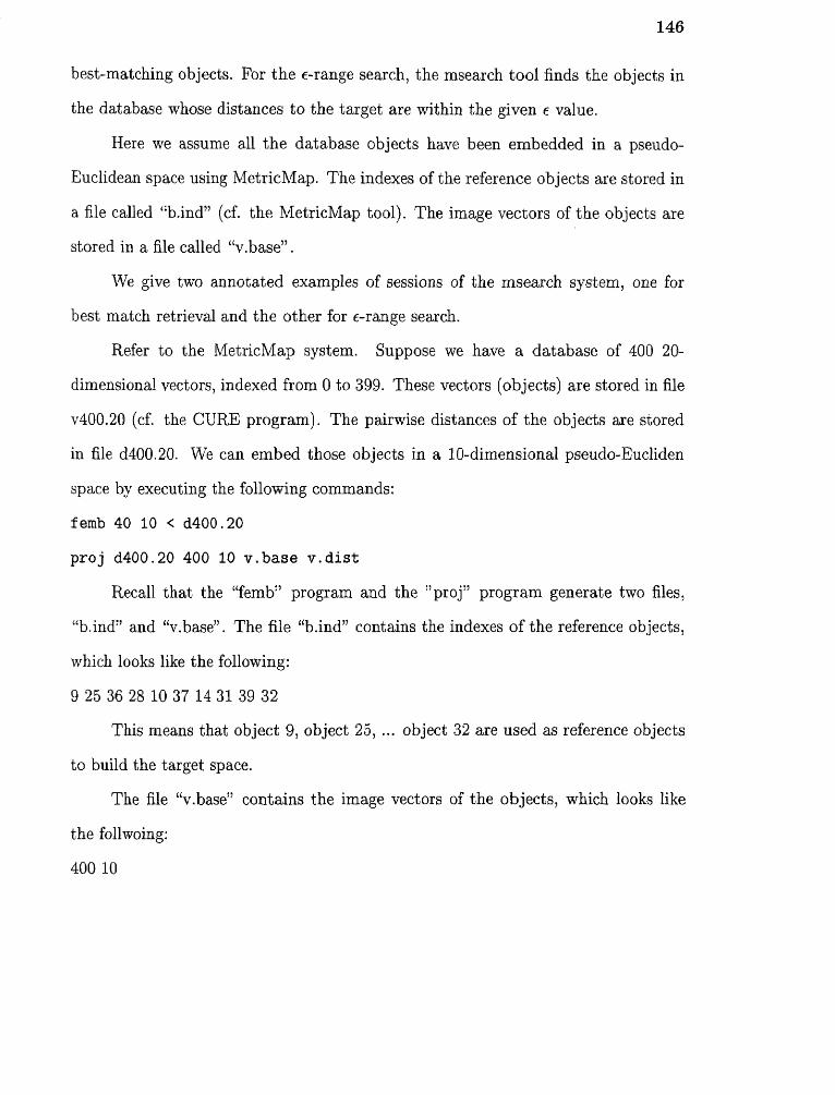
146

best-matching objects. For the c-range search, the msearch tool finds the objects in

the database whose distances to the target are within the given c value.

Here we assume all the database objects have been embedded in a pseudo-

Euclidean space using MetricMap. The indexes of the reference objects are stored in

a file called "b.ind" (cf. the MetricMap tool). The image vectors of the objects are

stored in a file called "v.base".

We give two annotated examples of sessions of the msearch system, one for

best match retrieval and the other for c-range search.

Refer to the MetricMap system. Suppose we have a database of 400 20-

dimensional vectors, indexed from 0 to 399. These vectors (objects) are stored in file

v400.20 (cf. the CURE program). The pairwise distances of the objects are stored

in file d400.20. We can embed those objects in a 10-dimensional pseudo-Eucliden

space by executing the following commands:

femb 40 10 < d400.20

proj d400.20 400 10 v.base v.dist

Recall that the "femb" program and the "proj" program generate two files,

"b.ind" and "v.base". The file "b.ind" contains the indexes of the reference objects,

which looks like the following:

9 25 36 28 10 37 14 31 39 32

This means that object 9, object 25, ... object 32 are used as reference objects

to build the target space.

The file "v.base" contains the image vectors of the objects, which looks like

the follwoing:

400 10

147

0.0000 0.0000 0.0000 0.0000 0.00000.0000 0.0000 0.0000 0.0000 0.0000

-2.5781 -2.1680 0.5737 2.0081 -0.7672-0.0987 0.2544 -0.3053 0.3483 0.0392-2.3080 0.8428 0.4520 0.8193 -0.87530.0016 0.4910 -0.0696 -0.2953 -0.2928

-1.6848 -0.4318 1.1193 2.0989 0.62110.3638 0.1002 0.5503 0.7714 0.5975

-3.1964 -0.4338 0.3476 -1.4289 -1.54070.6868 1.0198 0.1987 0.1276 -0.3175

The number 400 indicates that there are 400 vectors. The number 10 indicates

that these are 10-dimensional vectors. Each line of this file represents the coordinates

of an image vector in the pseudo-Euclidean space.

Now suppose we are given a target object in a file called "target". For example,

the data in the target file looks like the following:

-2.9375 -1.8045 -2.4635 -2.8335 -1.5975-1.9245 -1.6905 -2.5165 -2.7335 -1.46450.9480 -0.0230 0.5400 -0.3580 -0.01800.0440 0.7980 -0.7720 0.0490 -0.8840

To find the best match of the target, type the command:

msearch -b target

The output on the screen looks like the following:

The nearest neighbor of the target is object with the index 111.

Basically, the msearch tool first computes the distances from the target to the

reference objects stored in the file bind. Based on these distances, the tool is able to

embed the target in the pseudo-Euclidean space. The tool then finds best matches

in the pseudo-Euclidean space.

148

For є-range search, suppose we want to find objects that are within distance

2 of the target object stored in the file "target". One may type in the following

command:

msearch -r target 2

The output looks like the following:

The data objects that are within distance 2 of the target have indexes 111, 124, 158,

180.

To speed up search in the target space, we have implemented the VA-file

technique introduced by R. Webber et. al. in a paper entitled "A quantitative

Analysis and Performance Study for Similarity-Search Methods in High-Dimensional

Spaces" which appeared in the Proc. of VLDB'98.

CHAPTER 7

SUMMARY OF THE THESIS AND FUTURE WORK

7.1 Summary

We introduced an approach to finding active patterns in 3D graphs. Our approach is

an extension of the geometric hashing technique originally proposed by Lamden and

Wolfson [48, 49] for tackling computer vision problems. Major differences between

our technique and the previously published geometric hashing technique are listed

below.

• The existing geometric hashing technique considers every triplet of points in the

data object as a reference system, and therefore the records in the hash table are

highly redundant. For an object with n nodes, it will produce (n — 3) >

entries in the hash table. In contrast, our approach produces only

entries. In the on-line phase, the geometric hashing technique runs in time

0 (0) , while our approach runs in time 0(n3 ).

• Our approach divides an object into substructures. Thus it is capable of

dealing with substructure matches in which two substructures are rotatable

with respect to each other via a common edge. This phenomenon occurs

frequently in scientific data such as chemical compounds.

• The geometric hashing technique is sensitive to errors [34, 70]. Intuitively,

this is because the hash table addresses are calculated based on linear trans-

formation. In contrast, our approach simply uses lengths of line segments to

calculate the hash table addresses. Thus our approach can tolerate certain

errors caused by the inaccuracy of measurement.

149

150

We also presented a new data structure for data clustering and data mining.

Our contributions include:

• the development of a framework that utilizes sampling and the global knowledge

of the data set to optimize the vector representation;

• the development of a general projection formula for both an embeddable new

object and an unembeddable new object;

• estimating precisely the errors incurred by dimensionality reduction in pseudo-

Euclidean space.

7.2 Future Work

Our future work includes:

• the application of the three dimensional discovery algorithm to protein data

and developing new algorithms for protein clustering;

• the development of efficient algorithms based on the proposed index structure

to facilitate fast similarity search in metric spaces.

REFERENCES

1. E. E. Abola, F. C. Bernstein, S. H. Bryant, T. F. Koetzle, and J. Weng,"Protein data bank," in Crystallographic Databases — InformationContents, Software Systems, Scientific Applications (F. H. Allen,G. Bergerhoff, and R. Sievers, eds.), Data Commission of the Interna-tional Union of Crystallography, pp. 107-132, 1987.

2. R. Agrawal, J. Gehrke, D. Gunopulos, and P. Raghavan, "Automatic subspaceclustering of high dimensional data for datamining applications," inProceedings of the 1998 ACM SIGMOD International Conference onManagement of Data, Seattle, Washington, pp. 237-248, June 1998.

3. R. Agrawal, S. Ghosh, T. Imielinski, B. Iyer, and A. Swami, "An intervalclassifier for database mining applications," in Proceedings of the18th International Conference on Very Large Data Bases, Vancouver,Canada, pp. 560-573, Aug. 1992.

4. R. Agrawal, C. Faloutsos, and A. Swami, "Efficient similarity search insequence databases," Lecture Notes in Computer Science, vol. 730,pp. 69-84, 1993.

5. R. Baeza-Yates, W. Canto, U. Manber, and S. Wu, "proximity matching usingfixed-queries trees," in Combinatorial Pattern Matching, Lecture Notesin Computer Science, pp. 198-212, June 1994.

6. D. H. Ballard, "Generalizing the hough transform to detect arbitrary shapes,"Pattern Recognition, vol. 13, no. 2, pp. 111-122, 1981.

7. S. Berchtold, C. Bohm, B. Braunmuller, D. A. Keim, and H.-P. Kriegel, "Fastparallel similarity search in multimedia databases," in Proceedings ofthe ACM SIGMOD International Conference on Management of Data,pp. 1-12, May 1997.

8. F. C. Bernstein, T. F. Koetzle, G. J. B. Williams, E. F. Meyer, M. D. Brice,J. R. Rodgers, 0. Kennard, T. Shimanouchi, and M. Tasumi, "Theprotein data bank: A computer-based archival file for macromolecularstructures," Journal of Molecular Biology, vol. 112, pp. 535-542, 1977.

9. 0. Bourdon and G. Medioni, "Object Recognition Using Geometric Hashingon the Connection Machine," in 10th International Conference onPattern Recognition: 16-21 June 1990, Atlantic City, New Jersey, USA:Proceedings (H. Freeman, ed.), 1109 Spring Street, Suite 300, SilverSpring, MD 20910, USA, pp. 596-600, IEEE Computer Society Press,1990.

151

152

10. G. Burel, H. Henocq, and J. Y. Catros, "Registration of 3D objects using linearalgebra," in Computer Vision, Virtual Reality and Robotics in Medicine(N. Ayache, ed.), Lecture Notes in Computer Science, Springer-Verlag,April 1995. ISBN 3-540-59120-6.

11. C. Burks, M. Cassidy, M. J. Cinkosky, K. E. Cumella, P. Gilna, J. E.-D.Hayden, G. M. Keen, T. A. Kelley, M. Kelly, D. Kristofferson, andJ. Ryals, "GenBank," Nucleic Acids Research, vol. 19, pp. 2221-2225,1991.

12. G. J. S. Chang, J. T. L. Wang, G. W. Chirn, and C. Y. Chang, "A visual-ization tool for pattern matching and discovery in scientific databases,"in Proceedings of the Eighth International Conference on SoftwareEngineering and Knowledge Engineering, Lake Tahoe, Nevada, June1996.

13. J. Chao, K. Minowa, and S. Tsujii, "Unsupervised learning of 3D objectsconserving global topological order," IEICE Transactions on Funda-mentals of Electronics, Communications and Computer Sciences,vol. E76-A, no. 5, pp. 749-53, May 1993.

14. J. Chao and J. Nakayama, "Cubical singular simplex model for 3D objectsand fast computation of homology groups," in Proceedings of the 13thInternational Conference on Pattern Recognition, vol. 4, IEEE Comput.Soc. Press, Los Alamitos, California, USA, pp. 190-4, 1996.

15. D. Conklin, Knowledge Discovery in Molecular Structure Databases, Ph.D.dissertation, Department of Computing and Information Science,Queen's University, Canada, 1995.

16. D. Conklin, "Machine discovery of protein motifs," Machine Learning, vol. 21,pp. 125-150, 1995.

17. D. Conklin, S. Fortier, and J. Glasgow, "Knowledge discovery in moleculardatabases," IEEE Transactions on Knowledge and Data Engineering,vol. 5, no. 6, pp. 985-987, 1993.

18. L. S. Davis and N. Roussopoulos, "Approximate pattern matching in a patterndatabase system," Information Systems, vol. 5, pp. 107-119, 1980.

19.L. Dehaspe, H. Toivonen, and R. D. King, "Finding frequent substructuresin chemical compounds," in Proceedings of the 4nd InternationalConference on Knowledge Discovery and Data Mining, New York, NewYork, pp. 30-36, Aug. 1998.

20. S. Djoko, D. J. Cook, and L. B. Holder, "An empirical study of domainknowledge and its benefits to substructure discovery," IEEE Trans-actions on Knowledge and Data Engineering, vol. 9, no. 4, pp. 575-586,1997.

153

21. R. 0. Duda and P. E. Hart, Pattern Classification and Scene Analysis, JohnWiley & Sons, Inc., New York, New York, 1973.

22. M. Ester, H.-P. Kriegel, J. Sander, and X. Xu, "A density-based algorithm fordiscovering clusters in large spatial databases with noise," in Proceedingsof the 2nd International Conference on Knowledge Discovery and DataMining, Portland, Oregon, pp. 226-231, Aug. 1996.

23. C. Faloutsos, Searching Multimedia Databases by Content, Kluwer AcademicPublishers, Norwell, Massachusetts, 1996.

24. C. Faloutsos and K.-I. Lin, "f astmap: A fast algorithm for indexing, data-mining and visualization of traditional and multimedia datasets," inProceedings of the 1995 ACM SIGMOD International Conference onManagement of Data, pp. 163-174, May 1995.

25.C. Faloutsos, M. Ranganathan, and Y. Manolopoulos, "Fast subsequencematching in time-series databases," in Proceedings of the 1 994ACM SIGMOD International Conference on Management of Data,Minneapolis, Minnesota, pp. 419-429, May 1994.

26.P. Finn, L. Kavraki, J.-C. Latombe, R. Motwani, C. Shelton, S. Venkatasub-ramanian, and A. Yao, "RAPID: Randomized pharmacophore identifi-cation for drug design," in Proceedings of the 13th International AnnualSymposium on Computational Geometry (SCG-97), New York, pp. 324-333, ACM Press, June 4-6, 1997.

27. D. Fischer, 0. Bachar, R. Nussinov, and H. J. Wolfson, "An efficient automatedcomputer vision based technique for detection of three dimensionalstructural motifs in proteins," J. Biomolec. Struct. Dynam., vol. 9, no. 4,pp. 769-789, 1992.

28. K. Fukunaga, Introduction to Statistical Pattern Recognition, Academic Press,Inc., San Diego, California, 1990.

29. H. N. Gabow, Z. Galil, and T. H. Spencer, "Efficient implementation of graphalgorithms using contraction," in Proceedings of the 25th Annual IEEESymposium on Foundations of Computer Science, pp. 347-357, 1984.

30. K. Gardels, "Open gis and on-line environmental libraries," ACM SIGMODRecord, vol. 26, no. 1, pp. 32-38, March 1997.

31. L. Godfarb, "A new approach to pattern recognition," in Progress in PatternRecognition (L. Kanal and A. Rosenfeld, eds.), vol. 2, North-Holland,Amsterdam, pp. 241-402, 1985.

32. G. H. Golub and C. F. V. Loan, Matrix Computations, The Johns HopkinsUniversity Press, Baltimore, Maryland, 1996.

154

33. W. Greub, Linear Algebra, Springer-Verlag, Inc., New York, New York, 1975.

34. W. E. L. Grimson, D. P. Huttenlocher, and D. W. Jacobs, "Affine matchingwith bounded sensor error: Study of geometric hashing and alignment,"Technical Memo AIM-1250, Massachusetts Institute of Technology,Artificial Intelligence Laboratory, August 1991.

35. P. Grossmann, "From 3D line segments to objects and spaces," in CVPR '89(IEEE Computer Society Conference on Computer Vision and PatternRecognition, San Diego, CA, June 4-8, 1989), Washington, DC.,pp. 216-221, Computer Society Press, June 1989.

36. S. Guha, R. Rastogi, and K. Shim, "CURE: An efficient clustering algorithmfor large databases," in Proceedings of the 1998 ACM SIGMOD Interna-tional Conference on Management of Data, Seattle, Washington, pp. 73-84, June 1998.

37. R. W. Hamming, "Error detecting and error correcting codes," The Bell SystemTechnical Journal, vol. 29, no. 2, pp. 147-160, 1950.

38. J. C. Hart, W. O. Cochran, and P. J. Flynn, "Similarity hashing: A computervision solution to the inverse problem of linear fractals," Presented atthe NATO Advanced Study Institute on Fractal Image Encoding andAnalysis, Trondheim, Norway, July 1995, September 1995.

39. Y. C. Hecker and R. M. Bolle, "On geometric hashing and the generalizedHough transform," IEEE Trans. Systems, Man, and Cybernetics, vol. 24,no. 9, pp. 1328-1338, September 1994.

40. L. Hunter, ed., Artificial Intelligence and Molecular Biology, AAAI Press/TheMIT Press, Menlo Park, California, 1993.

41. R. W. Irving and C. B. Fraser, "Two algorithms for the longest common subse-quence of three (or more) strings," in Combinatorial Pattern Matching,Lecture Notes in Computer Science, 6i4 (A. Apostolico, M. Crochemore,Z. Galil, and U. Manber, eds.), Springer-Verlag, pp. 211-226, 1992.

42. A. K. Jain and R. C. Dubes, Algorithms for Clustering Data, Prentice Hall,Englewood Cliffs, New Jersey, 1988.

43. K. Kanatani, "3d euclidean versus 2D non-euclidean: Two approaches to 3Drecovery from images," IEEE Transactions on Pattern Analysis andMachine Intelligence, vol. 11, pp. 329-332, 1989.

44. L. Kaufman and P. J. Rousseeuw, Finding Groups in Data: An Introduction toCluster Analysis, John Wiley & Sons, Inc., New York, New York, 1990.

45. J. L. Kelley, General Topology, D. Van Nostrand Company, Inc., Princeton,New Jersey, 1955.

155

46. D. Keren, J. Subrahmonia, and D. B. Cooper, "Integrating algebraic curvesand surfaces, algebraic invariants and Bayesian methods for 2D and3D object recognition," Lecture Notes in Computer Science, vol. 825,pp. 493-498, 1994.

47. A. Krotopoulou, P. Spirakis, D. Terpou, and A. Tsakalidis, "A conceptualdatabase approach for modelling 3D objects of irregular geometry,"Lecture Notes in Computer Science, vol. 856, pp. 290-299, 1994.

48. Y. Lamdan, J. T. Schwartz, and H. J. Wolfson, "Object recognition by affineinvariant matching," in CVPR'88 (IEEE Computer Society Conferenceon Computer Vision and Pattern Recognition, Ann Arbor, MI, June 5-9, 1988), Washington, DC., pp. 335-344, Computer Society Press, June1988.

49. Y. Lamdan and H. J. Wolfson, "Geometric hashing: A general and efficientmodel-based recognition scheme," in Second International Conferenceon Computer Vision, Innesbrook Resort, Tampa, Florida, pp. 238-249,IEEE Computer Society Press, December 1988.

50. P. D. Lax, Linear Algebra, John Wiley & Sons, Inc., New York, New York,1997.

51. H. Mannila and H. Toivonen, "Levelwise search and borders of theories inknowledge discovery," Data Mining and Knowledge Discovery, vol. 1,no. 3, pp. 241-258, 1997.

52. J. E. W. Mayhew and J. P. Frisby, 3d Model Recognition From StereoscopicCues, MIT Press, Cambridge, Massachusetts, 1989.

53. J. A. McHugh, Algorithmic Graph Theory, Prentice Hall, Englewood Cliffs,New Jersey, 1990.

54. R. S. Michalski and R. E. Stepp, "Learning from observation: Conceptualclustering," in Machine Learning: An Artificial Intelligence Approach,volume I (R. S. Michalski, J. G. Carbonell, and T. M. Mitchell, eds.),Morgan Kaufmann, pp. 331-363, 1983.

55. M. Minsky and S. Papert, Perceptrons: An Introduction to ComputationalGeometry, M.I.T. Press, Cambridge, Massachusetts, 1969.

56. D. W. Murray and D. B. Cook, "Using the orientation of fragmentary 3D edgesegments for polyhedral object recognition," International Journal ofComputer Vision, vol. 2, no. 2, pp. 153-169, September 1988.

57. R. T. Ng and J. Han, "Efficient and effective clustering methods for spatialdata mining," in Proceedings of the 20th International Conference onVery Large Data Bases, Santiago, Chile, pp. 144-155, Sep. 1994.

156

58. R. Nussinov and H. J. Wolfson, "Efficient detection of three-dimensionalstructural motifs in biological macromolecules by computer visiontechniques.," in Proceedings of National Academy of Science of USA,vol. 88, pp. 10495-10499, December 1991.

59. I. Nystroem and G. Borgefors, "Synthesising objects and scenes using thereverse distance transformation in 2D and 3D," Lecture Notes inComputer Science, vol. 974, pp. 441-446, 1995.

60. J. M. Ortega, Matrix Theory, Plenum Press, New York, New York, 1987.

61. X. Pennec and N. Ayache, "An 0(n2) algorithm for 3D substructure matchingof proteins," in First International Workshop on Shape and PatternMatching in Computational Biology (A. Califano, I. Rigoutsos and H. J.Wolson, eds.), pp. 25-40, June 1994.

62. J. Ponce and D. J. Kriegman, "On recognizing and positioning curved 3Dobjects from image contours," in Image Understanding Workshop (PaloAlto, CA, May 23-26, 1989), San Mateo, CA, pp. 461-470, DefenseAdvanced Research Projects Agency, Morgan Kaufmann, 1989.

63. I. Rgoutsos and R. Hummel, "On a parallel implementation of geometrichashing on the connection machine," Tech. Rep. TR-554, Departmentof Computer Science, New York University, April 1991.

64. W.-F. Riekert, R. Mayer-Foll, and G. Wiest, "Management of data and servicesin the environmental information system (uis) of baden-wurttemberg,"ACM SIGMOD Record, vol. 26, no. 1, pp. 22-26, March 1997.

65. I. Rigoutsos and R. Hummel, "Scalable parallel geometric hashing forhypercube SIMD architechtures," Technical Report TR-553, New YorkUniversity, Jan. 1991.

66. I. Rigoutsos, D. Platt, and A. Califano, "Flexible substructure matching in verylarge databases of 3D-molecular information," research report, IBM T.J. Watson Research Center, 1996.

67. J. Sadowski and J. Gasteiger, "From atoms and bonds to three-dimensionalatomic coordinates: Automatic model builders," Chemical Reviews,vol. 93, pp. 2567-2581, 1993.

68. F. Sandakly and G. Giraudon, "Reasoning strategies for 3D object detection,"in IEEE International Symposium on Computer Vision, November 1995.

69. D. Sankoff and J. B. Kruskal, eds., Time Warps, String Edits, and Macro-molecules: The Theory and Practice of Sequence Comparison, Addison-Wesley, Reading, Massachusetts, 1983.

157

70. K. B. Sarachik, "Limitations of geometric hashing in the presence ofgaussian noise," Technical Memo AIM-1395, Massachusetts Institute ofTechnology, Artificial Intelligence Laboratory, October 1992.

71. J. Serra, ed., Image Analysis and Mathematical Morphology, Academic Press,New York, New York, 1982.

72. B. A. Shapiro and J. Navetta, "A massively parallel genetic algorithm forRNA secondary structure prediction," Journal of Supercomputing, vol. 8,pp. 195-207, 1994.

73. D. Shasha, J. T. L. Wang, K. Zhang, and F. Y. Shih, "Exact andapproximate algorithms for unordered tree matching," IEEE Trans-actions on Systems, Man and Cybernetics, vol. 24, no. 4, pp. 668-678,April 1994.

74. D. Shasha and T. L. Wang, "New techniques for best-match retrieval," ACMTransactions on Information Systems, vol. 8, no. 2, pp. 140-158, April1990.

75. D. Shasha and K. Zhang, "Fast algorithms for the unit cost editing distancebetween trees," Journal of Algorithms, vol. 11, no. 4, pp. 581-621, 1990.

76. A. Shashua, "On geometric and algebraic aspects of 3D affine and projectivestructures from perspective 2D views," Lecture Notes in ComputerScience, vol. 825, pp. 127-132, 1994.

77. G. Sheikholeslami, S. Chatterjee, and A. Zhang, "WaveCluster: A multi-resolution clustering approach for very large spatial databases," inProceedings of the 24th International Conference on Very Large DataBases, New York, New York, pp. 428-439, Aug. 1998.

78. A. F. Smeaton and C. J. V. Rijsbergen, "The nearest neighbor problem ininformation retrieval: an algorithm using upperbounds," ACM SIGIRForum, vol. 16, pp. 83-87, 1981.

79. R. Steinmetz and K. Nahrstedt, eds., Multimedia: Computing, Communi-cations and Applications, Prentice Hall, Englewood Cliffs, New Jersey,1995.

80. R. R. Stoll, Linear Algebra and Matrix Theory, McGraw-Hill, Inc., New York,1952.

81. R. L. Tatusov, S. F. Altschul, and E. V. Koonin, "Detection of conservedsegments in proteins: iterative scanning of sequence databases withalignment blocks," Proceedings of National Academy of Science of USA,vol. 91, pp. 12091-12095, 1994.

158

82. I. I. Vaisman, A. Tropsha, and W. Zheng, "Compositional preferences inquadruplets of nearest neighbor residues in protein structures: Statisticalgeometry analysis," in Proceedings of IEEE International Join Symposiaon Intelligence and Systems, Rockville, Maryland, pp. 163-168, Aug.1998.

83. R. A. Wagner and M. J. Fischer, "The string-to-string correction problem,"Journal of the ACM, vol. 21, no. 1, pp. 168-173, Jan. 1974.

84. J. T. L. Wang, G. W. Chirn, T. G. Marr, B. A. Shapiro, D. Shasha, andK. Zhang, "Combinatorial pattern discovery for scientific data: Somepreliminary results," in Proceedings of the 1994 ACM SIGMOD Inter-national Conference on Management of Data, Minneapolis, Minnesota,pp. 115-125, May 1994.

85. J. T. L. Wang, T. G. Marr, D. Shasha, B. Shapiro, and G. W. Chirn,"Discovering active motifs in sets of related protein sequences andusing them for classification," Nucleic Acids Research, vol. 22, no. 14,pp. 2769-2775, 1994.

86. J. T. L. Wang, T. G. Marr, D. Shasha, B. Shapiro, G. W. Chirn, and T. Y.Lee, "Complementary classification approaches for protein sequences,"Protein Engineering, vol. 9, no. 5, pp. 381-386, 1996.

87. J. T. L. Wang, B. A. Shapiro, and D. Shasha, eds., Pattern Discoveryin Biomolecular Data: Tools, Techniques and Applications, OxfordUniversity Press, New York, New York, Mar. 1999.

88. J. T. L. Wang, B. A. Shapiro, D. Shasha, K. Zhang, and C.-Y. Chang,"Automated Discovery of Active Motifs in Multiple RNA SecondaryStructures," in Proceedings of the 2nd International Conference onKnowledge Discovery and Data Mining, Portland, Oregon, pp. 70-75,Aug. 1996.

89. J. T. L. Wang, D. Shasha, G. Chang, L. Relihan, K. Zhang, andG. Patel, "Structural matching and discovery in document databases,"in Proceedings of the 1997 ACM SIGMOD International Conference onManagement of Data, Tucson, Arizona, pp. 560-563, May 1997.

90. J. T. L. Wang, K. Zhang, and G. W. Chirn, "Algorithms for approximate graphmatching," Information Sciences, vol. 82, pp. 45-74, 1995.

91. J. T. L. Wang, K. Zhang, K. Jeong, and D. Shasha, "A system forapproximate tree matching," IEEE Transactions on Knowledge andData Engineering, vol. 6, no. 4, pp. 559-571, August 1994.

92. J. T. L. Wang, X. Wang, K.-I. Lin, D. Shasha, B. A. Shapiro, and K. Zhang,"Evaluating a class of distance-mapping algorithms for data mining

159

and clustering," in Proceedings of the ACM SIGKDD InternationalConference on Knowledge Discovery and Data Mining, San Diego,California, pp. 307-311, August 1999.

93. T. L. Wang and D. Shasha, "Query processing for distance metrics," inProceedings of the 16th International Conference on Very Large DataBases, Brisbane, Australia, pp. 602-613, Aug. 1990.

94. W. Wang, J. Yang, and R. Muntz, "STING: A statistical information gridapproach to spatial data mining," in Proceedings of the 23rd Interna-tional Conference on Very Large Data Bases, Athens, Greece, pp. 186-195, Aug. 1997.

95. X. Wang and J. T. L. Wang, "Fast similarity search in databases of 3d objects,"in Proceedings of the 10th IEEE International Conference on Tools withArtifical Intelligence, Taipei, Taiwan, pp. 16-23, November 1998.

96. X. Wang, J. T. L. Wang, D. Shasha, B. A. Shapiro, S. Dikshitulu, I. Rigoutsos,and K. Zhang, "Automated discovery of active motifs in three dimen-sional molecules," in Proceedings of the 3rd International Conferenceon Knowledge Discovery and Data Mining, Newport Beach, California,pp. 89-95, August 1997.

97. X. Wang, J. T. L. Wang, K.-I. Lin, D. Shasha, B. A. Shapiro, andK. Zhang, "Implementation and evaluation of an index structure fordata clustering," Knowledge and Information Systems: An InternationalJournal, To appear, 2000.

98. X. Wang, J. T. L. Wang, D. Shasha, B. Shapiro, I. Rigoutsos, andK. Zhang, "Finding patterns in three dimensional graphs: Algorithmsand applications to scientific data mining," Research Report CIS-99-04,Computer and Information Science Department, New Jersey Institute ofTechnology, 1999.

99. H. J. Wolfson, "Model-based object recognition by geometric hashing,"in Proceedings of the 1st European Conference on Computer Vision(0. Faugeras, ed.), vol. 427 of LNCS, Berlin, pp. 526-536, Springer,April 1990.

100. M. C. Yang and W. H. Tsai, "Recognition of single 3D curved objects using2D cross-sectional slice shapes," Image and Vision Computing, vol. 7,pp. 210-216, 1989.

101. Y. Yang, K. Zhang, X. Wang, J. T. L. Wang, and D. Shasha, "An approximateoracle for distance in metric spaces," in Combinatorial Pattern Matching(M. Farach-Colton, ed.), Lecture Notes in Computer Science, 1448,Springer-Verlag, pp. 104-117, 1998.

160

102. B.-K. Yi, H. V. Jagadish, and C. Faloutsos, "Efficient retrieval of similar timesequences under time warping," in Proceedings of 14th IEEE Interna-tional Conference on Data Engineering, Orlando, Florida, pp. 201-208,Feb. 1998.

103. K. Zhang, D. Shasha, and J. T. L. Wang, "Fast serial and parallel algorithmsfor approximate tree matching with VLDC's," in Proc. of the 3rdAnnual Symposium on Combinatorial Pattern Matching (A. Apostolico,M. Crochemore, Z. Galil, and U. Manber, eds.), Lecture Notes inComputer Science, 644, Springer-Verlag, pp. 151-161, 1992.

104. K. Zhang, J. T. L. Wang, and D. Shasha, "On the editing distance betweenundirected acyclic graphs," International Journal of Foundations ofComputer Science, Special Issue on Computational Biology, vol. 7, no. 1,pp. 43-57, 1996.

105. T. Zhang, R. Ramakrishnan, and M. Livny, "BIRCH: An efficient dataclustering method for very large databases," in Proceedings of the1996 ACM SIGMOD International Conference on Management of Data,Montreal, Quebec, Canada, pp. 103-114, June 1996.