Embed Size (px)
Citation preview
© Boardworks Ltd 20061 of 61 © Boardworks Ltd 20061 of 61
A2-Level Maths: Statistics 2for Edexcel
S2.2 Continuous random variables
This icon indicates the slide contains activities created in Flash. These activities are not editable.
For more detailed instructions, see the Getting Started presentation.
© Boardworks Ltd 20062 of 61
Co
nte
nts
© Boardworks Ltd 20062 of 61
Relative frequency histograms
Relative frequency histograms
Probability density functions
Mode
Cumulative distribution functions
Median and quartiles
Expectation
Variance

© Boardworks Ltd 20063 of 61
A histogram has the important property that the area of each bar is in proportion to the corresponding frequency.
A histogram with unequal widths can be drawn by plotting the frequency density on the vertical axis, where:
frequencyfrequency density =
class width
Relative frequency histograms
frequency densityrelative frequency density =
total frequency
A relative frequency histogram is one in which the area of a bar corresponds to the proportion of the data falling into the corresponding interval.
The relative frequency is defined as:

© Boardworks Ltd 20064 of 61
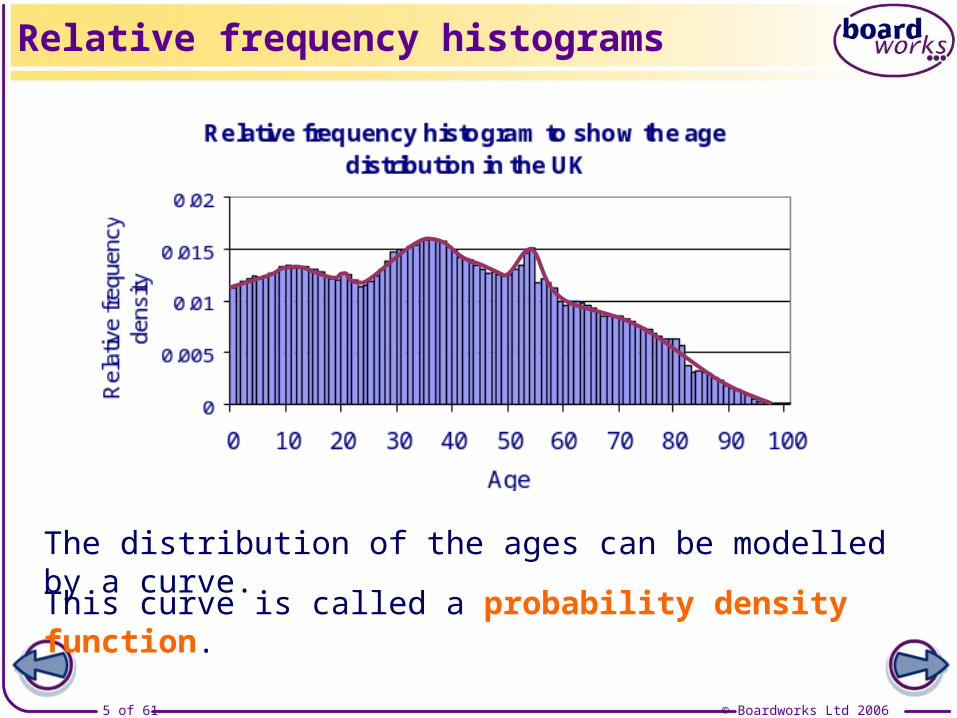
Example: The relative frequency histogram below shows the distribution of ages of the UK population.
Relative frequency histograms
The area of each bar corresponds to the proportion of the population with ages in that interval.
The total area of all the bars is 1.
© Boardworks Ltd 20065 of 61
The distribution of the ages can be modelled by a curve.
Relative frequency histograms
This curve is called a probability density function.
© Boardworks Ltd 20066 of 61
Co
nte
nts
© Boardworks Ltd 20066 of 61
Probability density functions
Relative frequency histograms
Probability density functions
Mode
Cumulative distribution functions
Median and quartiles
Expectation
Variance
© Boardworks Ltd 20067 of 61
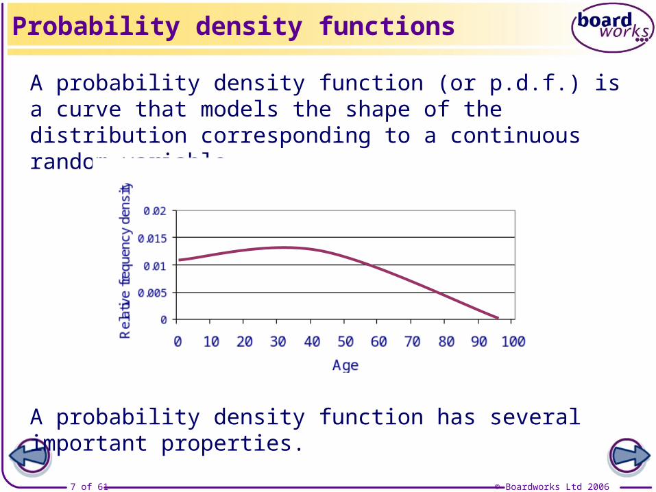
A probability density function (or p.d.f.) is a curve that models the shape of the distribution corresponding to a continuous random variable.
Probability density functions
A probability density function has several important properties.

© Boardworks Ltd 20068 of 61
If f(x) is the p.d.f corresponding to a continuous random variable X and if f(x) is defined for a ≤ x ≤ b then the following properties must hold:
f ( )b
a
x dx 1
i.e. the total area under a p.d.f. is 1.
Probability density functions
1.

© Boardworks Ltd 20069 of 61
If f(x) is the p.d.f. corresponding to a continuous random variable X and if f(x) is defined for a ≤ x ≤ b then the following properties must hold:
2.
Probability density functions
f ( ) x a x b 0 for
i.e. the graph of the p.d.f. never dips below the x-axis.
© Boardworks Ltd 200610 of 61
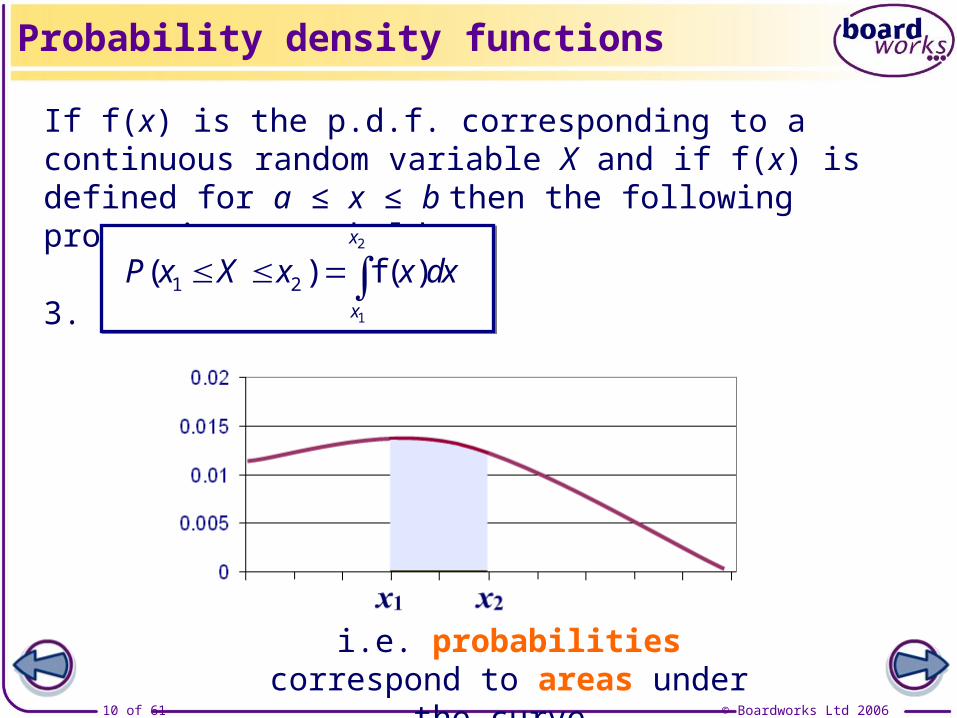
If f(x) is the p.d.f. corresponding to a continuous random variable X and if f(x) is defined for a ≤ x ≤ b then the following properties must hold:
3.
Probability density functions
( ) f ( )x
x
P x X x x dx 2
1
1 2
i.e. probabilities correspond to areas under the curve.
© Boardworks Ltd 200611 of 61
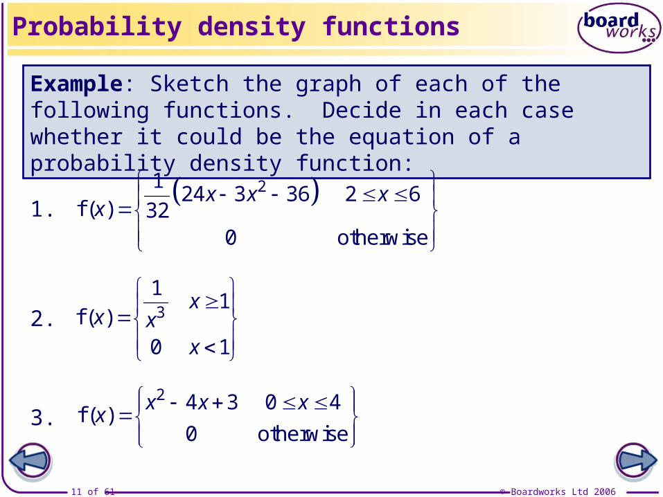
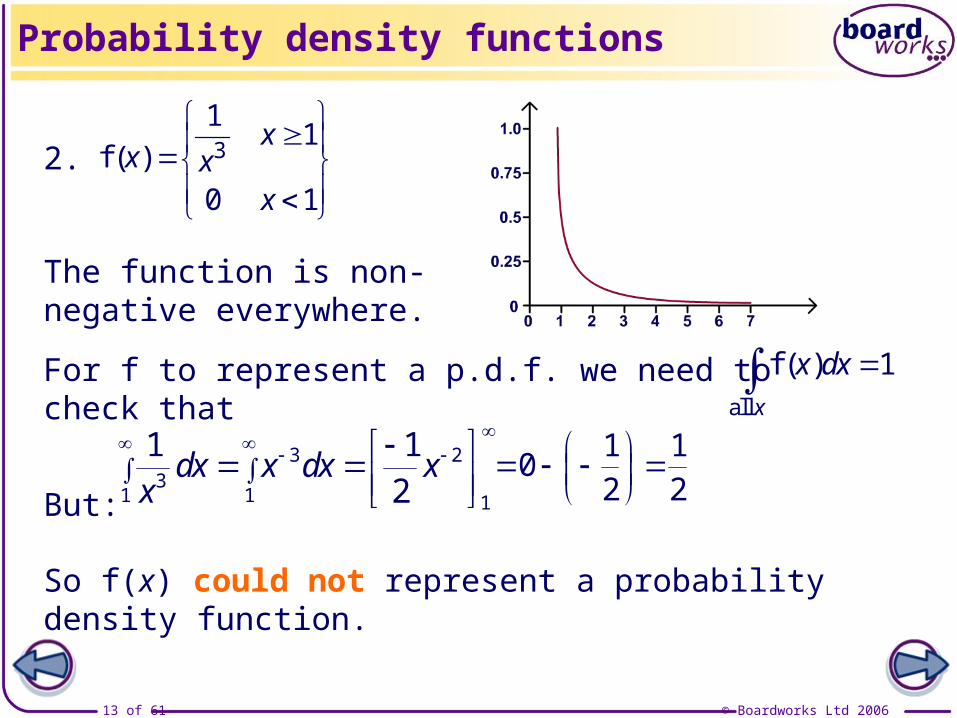
Example: Sketch the graph of each of the following functions. Decide in each case whether it could be the equation of a probability density function:
f ( )x
x xx
3
11
0 1
Probability density functions
f ( )x x x
x
2124 3 36 2 6
320 otherwise
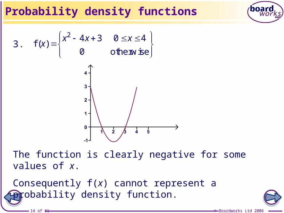
f ( )x x x
x
2 4 3 0 4
0 otherwise3.
2.
1.
© Boardworks Ltd 200612 of 61
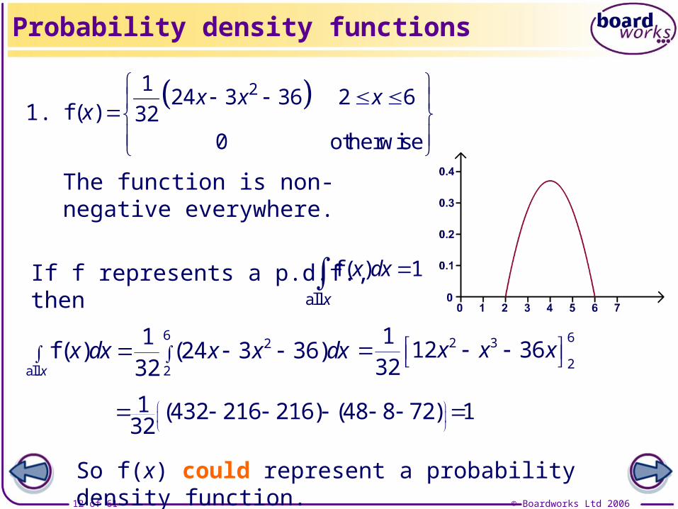
Probability density functions
The function is non-negative everywhere.
If f represents a p.d.f., thenall
f ( )x
x dx 1
allf ( ) ( )
xx dx x x dx
62
2
124 3 36
32
( ) ( )
1 432 216 216 48 8 72 132
So f(x) could represent a probability density function.
1. f ( )x x x
x
2124 3 36 2 6
320 otherwise
x x x 62 3
2
112 36
32
© Boardworks Ltd 200613 of 61
The function is non-negative everywhere.
For f to represent a p.d.f. we need to check that
But:
Probability density functions
dx x dx xx
3 2
31 1 1
1 12
all
f ( )x
x dx 1
So f(x) could not represent a probability density function.
2. f ( )x
x xx
3
11
0 1
1 10
2 2
© Boardworks Ltd 200614 of 61
Probability density functions
The function is clearly negative for some values of x.
Consequently f(x) cannot represent a probability density function.
f ( )x x x
x
2 4 3 0 4
0 otherwise3.
© Boardworks Ltd 200615 of 61
Probability density functions

© Boardworks Ltd 200616 of 61
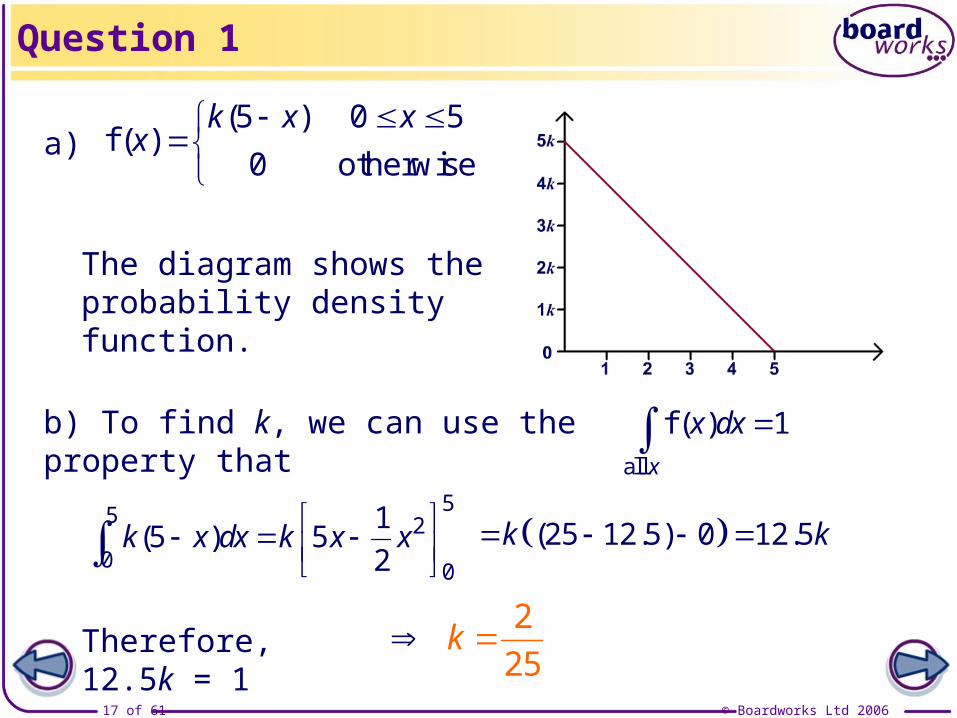
Question 1: A continuous random variable X is defined by the probability density function
( )f ( )
k x xx
5 0 5
0 otherwise
Question 1
a) Sketch the probability density function.
b) Find the value of the constant k.
c) Find P(1 ≤ X ≤ 3).
© Boardworks Ltd 200617 of 61
a)
The diagram shows the probability density function.
Question 1
( )k x dx k x x
55 2
0 0
15 5
2
2
25k Therefore, 12.5k = 1
b) To find k, we can use the property that
( )f ( )
k x xx
5 0 5
0 otherwise
all
f ( )x
x dx 1
( . )k k 25 12 5 0 12.5
© Boardworks Ltd 200618 of 61
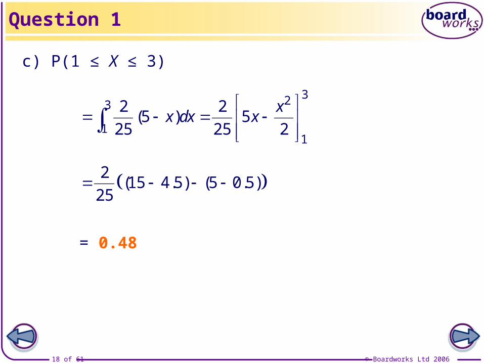
c) P(1 ≤ X ≤ 3)
( )
323
11
2 25 5
25 25 2
xx dx x
Question 1
= 0.48
( . ) ( . )2
15 4 5 5 0 525
© Boardworks Ltd 200619 of 61
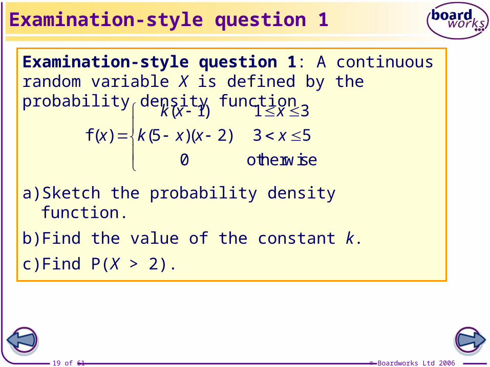
Examination-style question 1: A continuous random variable X is defined by the probability density function
Examination-style question 1
( )
f ( ) ( )( )
k x x
x k x x x
1 1 3
5 2 3 5
0 otherwise
a) Sketch the probability density function.
b) Find the value of the constant k.
c) Find P(X > 2).
© Boardworks Ltd 200620 of 61
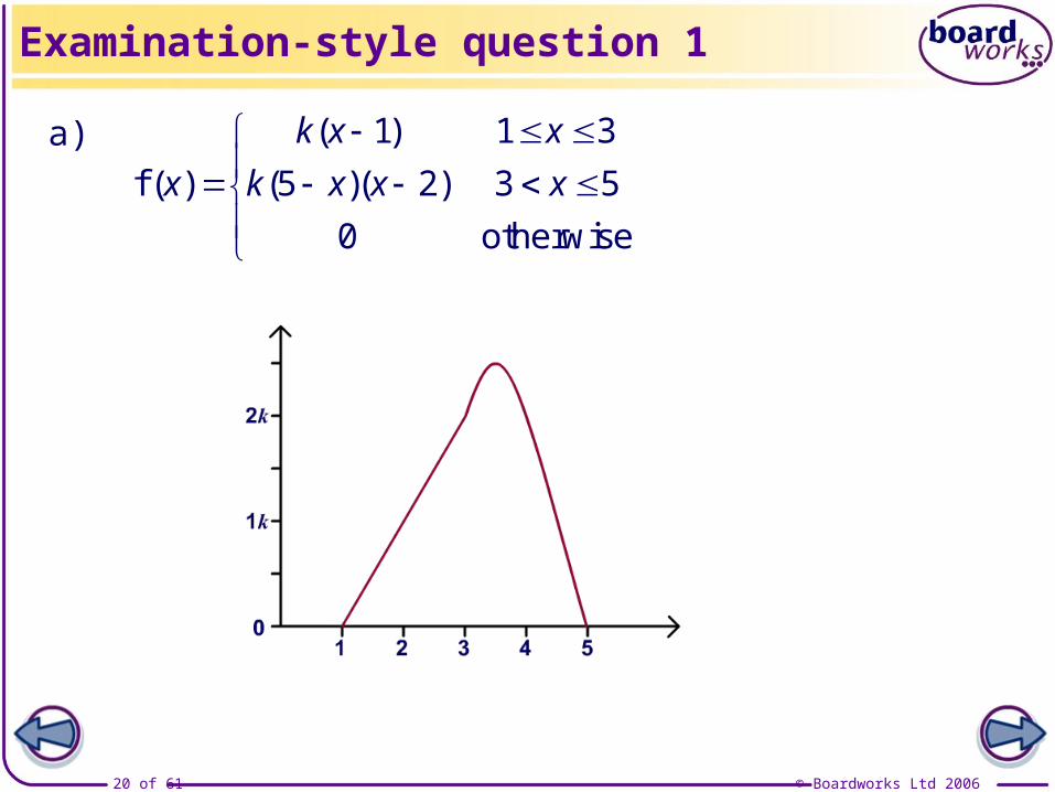
Examination-style question 1
a) ( )
f ( ) ( )( )
k x x
x k x x x
1 1 3
5 2 3 5
0 otherwise
© Boardworks Ltd 200621 of 61
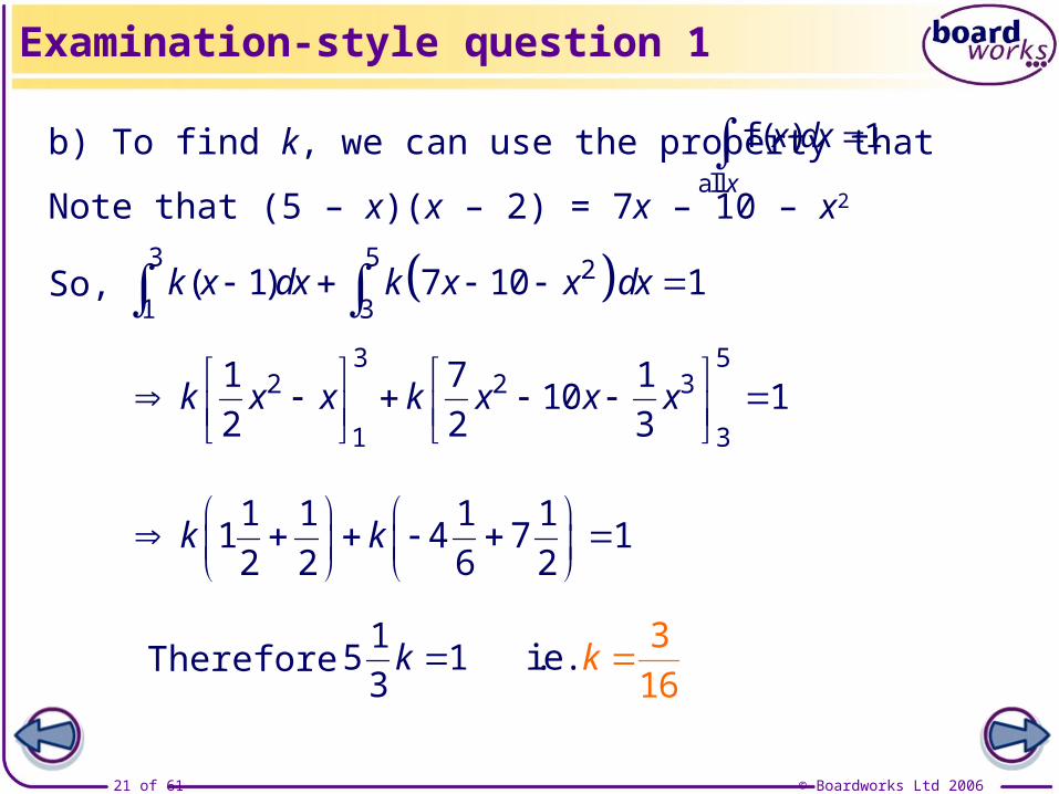
b) To find k, we can use the property that
Note that (5 – x)(x – 2) = 7x – 10 – x2
Examination-style question 1
3 52 2 3
1 3
1 7 110 1
2 2 3k x x k x x x
( )3 5 2
1 31 7 10 1k x dx k x x dx
1 1 1 11 4 7 1
2 2 6 2k k
15 1
3k Therefore
all
f ( )x
x dx 1
So,
1i.e.
3
6k
© Boardworks Ltd 200622 of 61
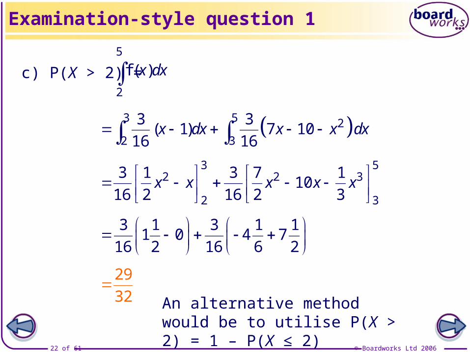
c) P(X > 2) =
Examination-style question 1
f ( )x dx5
2
x x x x x
3 52 2 3
2 3
3 1 3 7 110
16 2 16 2 3
( )3 5 2
2 3
3 31 7 10
16 16x dx x x dx
3 1 3 1 11 0 4 7
16 2 16 6 2
29
32 An alternative method would be to utilise P(X > 2) = 1 – P(X ≤ 2)

© Boardworks Ltd 200623 of 61
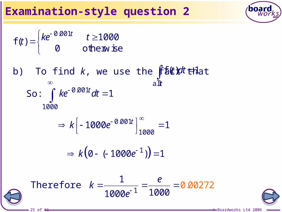
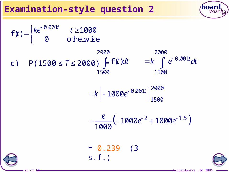
Examination-style question 2: The life, T hours, of an electrical component is modelled by the probability density function
a) Sketch the probability density function.
b) Find the value of the constant k.
c) Find P(1500 ≤ T ≤ 2000).
.f ( )
tke tt
0 001 10000 otherwise
Examination-style question 2
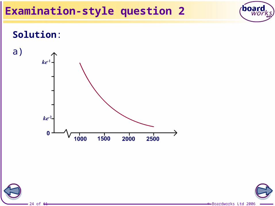
© Boardworks Ltd 200624 of 61
Examination-style question 2
Solution:
a)
© Boardworks Ltd 200625 of 61
b) To find k, we use the fact that f ( )t
t dt all
1
So:
Examination-style question 2
. tke dt
0 001
1000
1
. tk e
0 001
10001000 1
( )k e 10 1000 1
.e
ke
1
1
10
000100000272Therefore
.f ( )
tke tt
0 001 10000 otherwise
© Boardworks Ltd 200626 of 61
c) P(1500 ≤ T ≤ 2000) = .f ( ) tt dt k e dt
2000 20000 001
1500 1500
Examination-style question 2
. tk e 20000 001
15001000
.ee e 2 1 51000 1000
1000
= 0.239 (3 s.f.)
.f ( )
tke tt
0 001 10000 otherwise

© Boardworks Ltd 200627 of 61
Co
nte
nts
© Boardworks Ltd 200627 of 61
Mode
Relative frequency histograms
Probability density functions
Mode
Cumulative distribution functions
Median and quartiles
Expectation
Variance
© Boardworks Ltd 200628 of 61
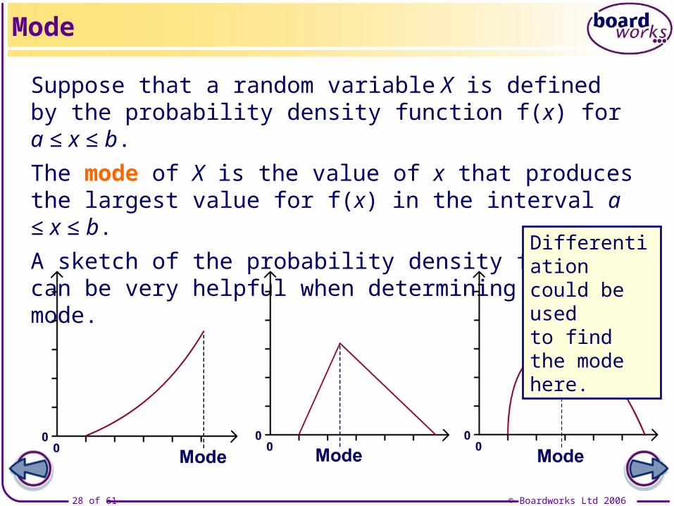
Suppose that a random variable X is defined by the probability density function f(x) for a ≤ x ≤ b.
The mode of X is the value of x that produces the largest value for f(x) in the interval a ≤ x ≤ b.
A sketch of the probability density function can be very helpful when determining the mode.
Mode
Differentiationcould be usedto find the mode here.

© Boardworks Ltd 200629 of 61
Example: A random variable X has p.d.f. f(x), where
Find the mode.
( )f ( ) x x xx
2 2 0 20 otherwise
Sketch of f(x):
Mode

© Boardworks Ltd 200630 of 61
Mode
The mode can be found using differentiation:
f ( ) f ( )x x x x x x 2 3 22 4 3
To find a turning point, we solve f ( )x 0
( )4 3 0x x Factorize:
f ( ) f ( )x x 434 6 4 8 4 0
Check that gives the maximum value: 43x
So the mode is . 43x
24 3 0x x
or 430x x
© Boardworks Ltd 200631 of 61
Co
nte
nts
© Boardworks Ltd 200631 of 61
Cumulative distribution functions
Relative frequency histograms
Probability density functions
Mode
Cumulative distribution functions
Median and quartiles
Expectation
Variance

© Boardworks Ltd 200632 of 61
The cumulative distribution function (c.d.f.) F(x) for a continuous random variable X is defined as
F(x) = P(X ≤ x).
Therefore, the c.d.f. is found by integrating the p.d.f..
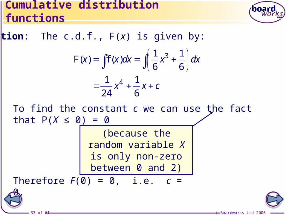
Example: A random variable X has p.d.f. f(x), where
f ( )x x
x
311 0 2
60 otherwise
Find the c.d.f. and find P(X < 1).
Cumulative distribution functions
© Boardworks Ltd 200633 of 61
Solution: The c.d.f., F(x) is given by:
F( ) f ( )x x dx x dx 31 1
6 6
Cumulative distribution functions
41 1
24 6x x c
To find the constant c we can use the fact that P(X ≤ 0) = 0
(because the random variable X is only non-zero between 0 and 2)
Therefore F(0) = 0, i.e. c = 0.
© Boardworks Ltd 200634 of 61
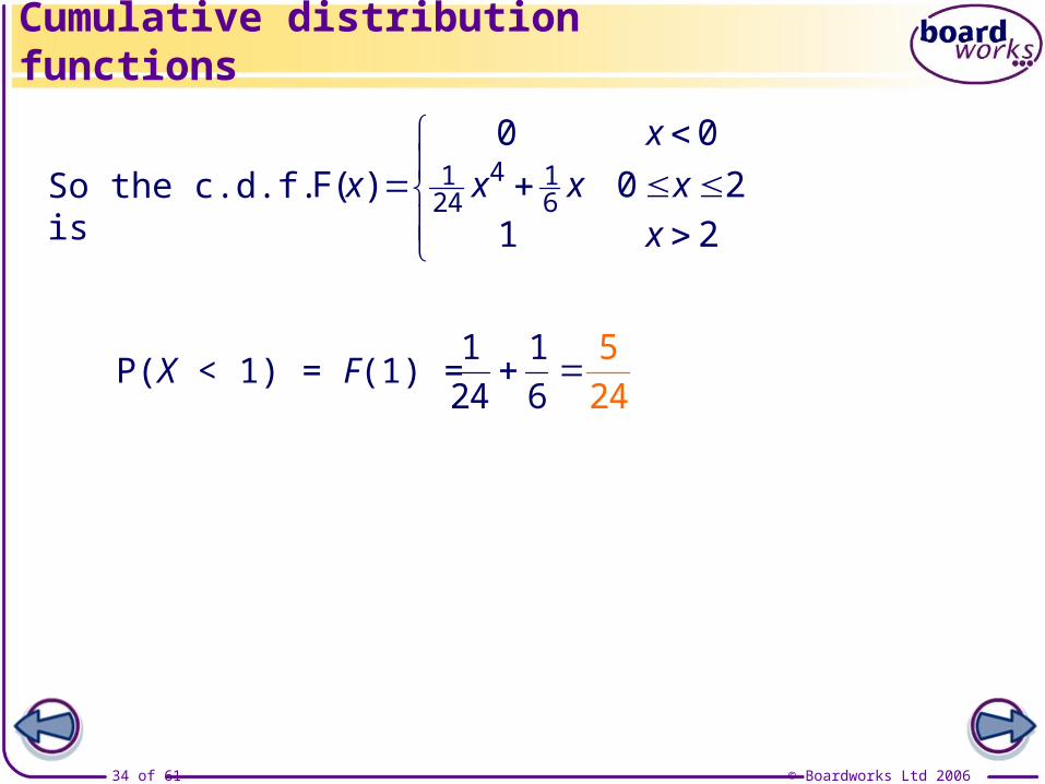
Cumulative distribution functions
So the c.d.f. is F( )
x
x x x x
x
41 124 6
0 0
0 21 2
P(X < 1) = F(1) =1 1
24 6
5
24

© Boardworks Ltd 200635 of 61
Co
nte
nts
© Boardworks Ltd 200635 of 61
Median and quartiles
Relative frequency histograms
Probability density functions
Mode
Cumulative distribution functions
Median and quartiles
Expectation
Variance
© Boardworks Ltd 200636 of 61
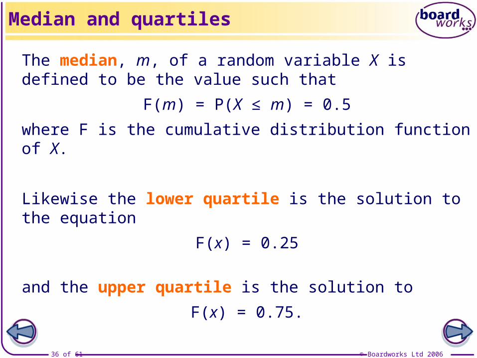
The median, m, of a random variable X is defined to be the value such that
F(m) = P(X ≤ m) = 0.5
where F is the cumulative distribution function of X.
Likewise the lower quartile is the solution to the equation
F(x) = 0.25
and the upper quartile is the solution to
F(x) = 0.75.
Median and quartiles

© Boardworks Ltd 200637 of 61
Median and quartiles
© Boardworks Ltd 200638 of 61
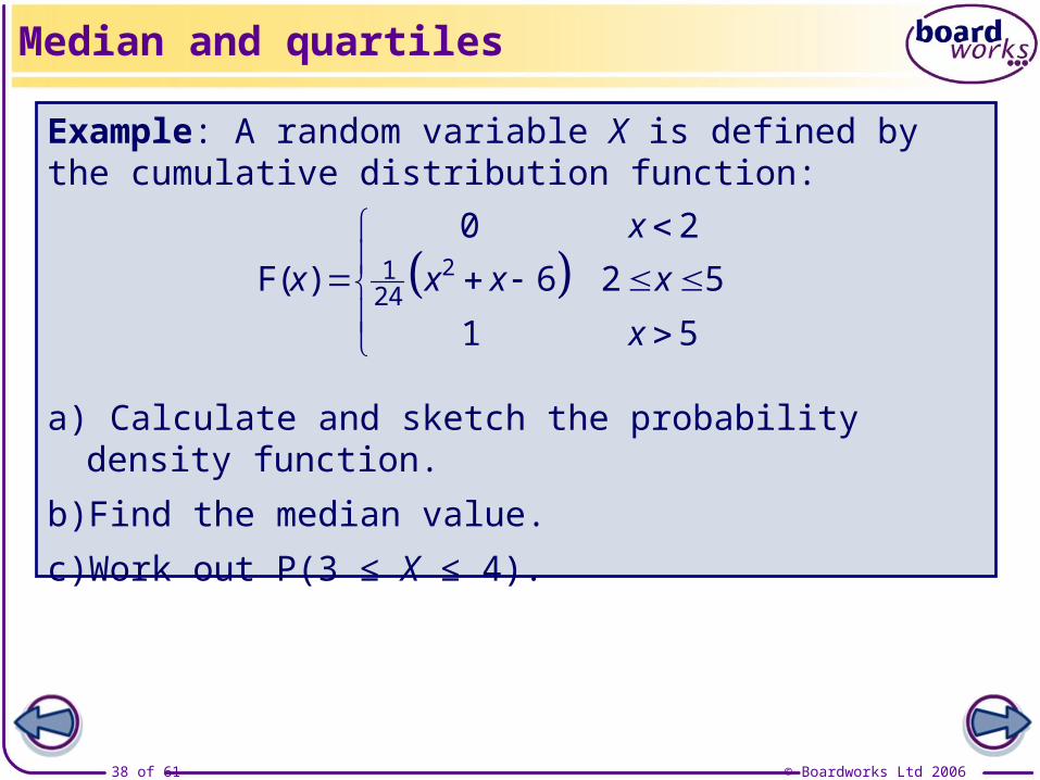
Example: A random variable X is defined by the cumulative distribution function:
F( ) 2124
0 2
6 2 5
1 5
x
x x x x
x
a) Calculate and sketch the probability density function.
b) Find the median value.
c) Work out P(3 ≤ X ≤ 4).
Median and quartiles

© Boardworks Ltd 200639 of 61
a) We can get the p.d.f. by differentiating the c.d.f.
f ( ) F ( )x x x 1 112 24
So the p.d.f. is
f ( )x x
x
1 112 24 2 5
0 otherwise
Sketch of f(x):
Median and quartiles

© Boardworks Ltd 200640 of 61
The median must be 3.77 (as the p.d.f. is only non-zero for values in the interval [2, 5]).
2 6 12m m
b) The median, m, satisfies F(m) = 0.5.
Therefore .2124 6 0 5m m
Median and quartiles
( )1 1 4 1 18
2m
2 18 0m m
.m m 4 77 or 3.77
© Boardworks Ltd 200641 of 61
Median and quartiles
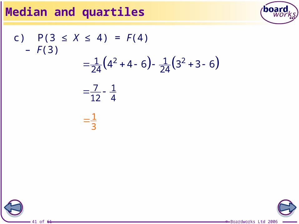
c) P(3 ≤ X ≤ 4) = F(4) – F(3)
2 21 124 244 4 6 3 3 6
13
7 112 4
© Boardworks Ltd 200642 of 61
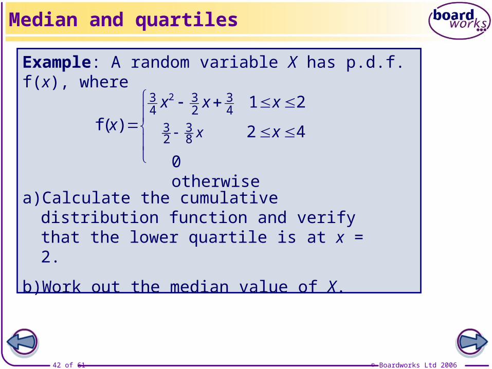
Example: A random variable X has p.d.f. f(x), where
f ( )x x x
x
23 3 34 2 4 1 2
a) Calculate the cumulative distribution function and verify that the lower quartile is at x = 2.
b) Work out the median value of X.
Median and quartiles
0 otherwise
x x 3 32 8 2 4
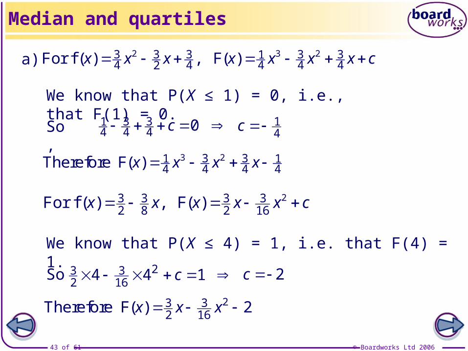
© Boardworks Ltd 200643 of 61
f ( ) F( )x x x x x x x c 2 3 23 3 3 3 314 4 4 4 42For ,
Median and quartiles
c 3 314 4 4 0
f ( ) , F( )x x x x x c 23 3 3 32 8 2 16For
We know that P(X ≤ 1) = 0, i.e., that F(1) = 0.
23 32 164 4 1c
F( )x x x x 3 23 31 14 4 4 4Therefore
We know that P(X ≤ 4) = 1, i.e. that F(4) = 1.
F( )x x x 23 32 16Therefore 2
So,
So 2c
a)
14c

© Boardworks Ltd 200644 of 61
Median and quartiles
F( )3 2
2
3 31 14 4 4 4
3 32 16
0 1
1 2
2 2 4
1 4
x
x x x xx
x x x
x
So
To verify that the lower quartile is 2, we simply need to check that F(2) = 0.25:
F( ) . 3 21 3 3 12 2 2 2 0 25
4 4 4 4
Therefore the lower quartile is 2.
© Boardworks Ltd 200645 of 61
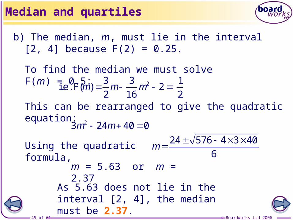
b) The median, m, must lie in the interval [2, 4] because F(2) = 0.25.
To find the median we must solve F(m) = 0.5:
F( )m m m 23 3 1i.e. 2
2 16 2This can be rearranged to give the quadratic equation:
23 24 40 0m m
Using the quadratic formula,
As 5.63 does not lie in the interval [2, 4], the median must be 2.37.
Median and quartiles
24 576 4 3 40
6m
m = 5.63 or m = 2.37

© Boardworks Ltd 200646 of 61
Co
nte
nts
© Boardworks Ltd 200646 of 61
Expectation
Relative frequency histograms
Probability density functions
Mode
Cumulative distribution functions
Median and quartiles
Expectation
Variance
© Boardworks Ltd 200647 of 61
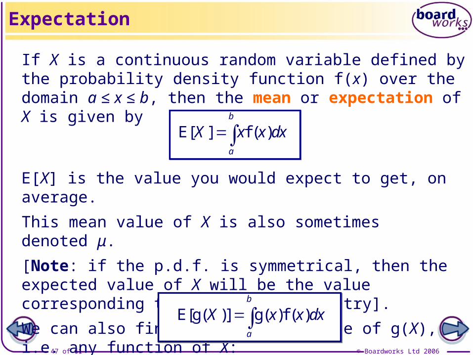
If X is a continuous random variable defined by the probability density function f(x) over the domain a ≤ x ≤ b, then the mean or expectation of X is given by
E[X] is the value you would expect to get, on average.
This mean value of X is also sometimes denoted μ.
[Note: if the p.d.f. is symmetrical, then the expected value of X will be the value corresponding to the line of symmetry].
We can also find the expected value of g(X), i.e. any function of X:
Expectation
[g( )] g( )f ( )b
a
X x x dxE
[ ] f ( )b
a
X x x dxE

© Boardworks Ltd 200648 of 61
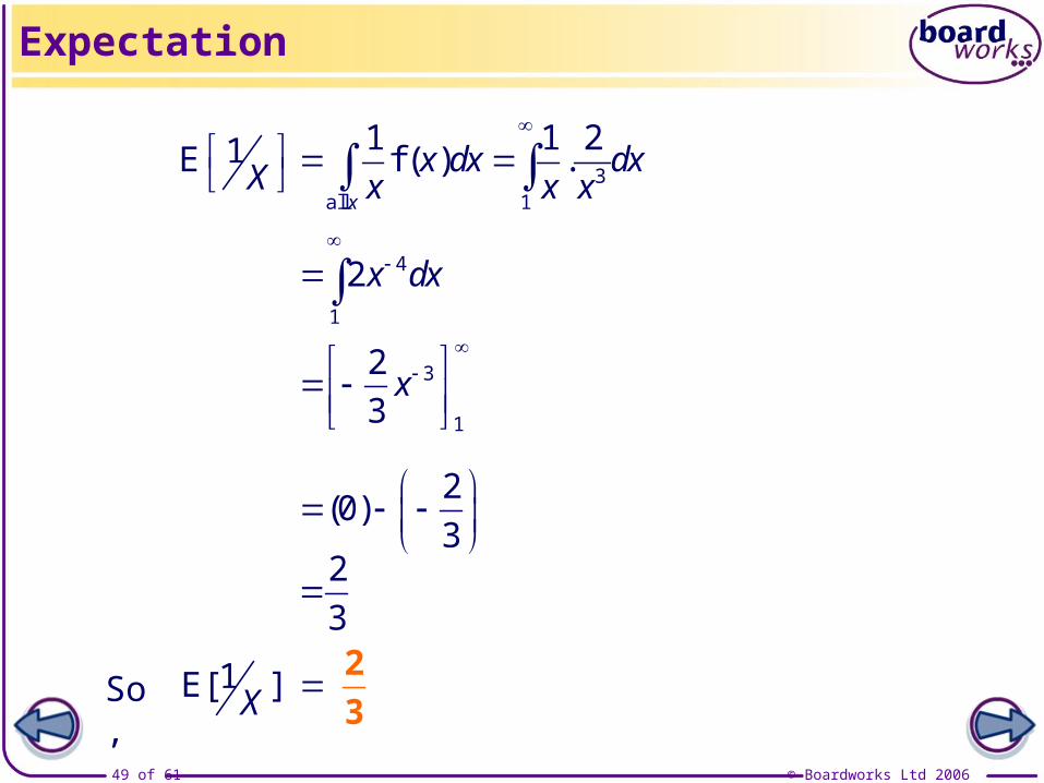
Example: A random variable X is defined by the probability density function
f ( )x
x x
3
21
0 otherwise
Calculate the value of E[X] and E[1/X].
[ ] f ( ) .x
X x x dx x dxx
3all 1
2E
21
2dx
x
Expectation
2 1
11
2 2x dx x
( ) ( )0 2 2
© Boardworks Ltd 200649 of 61
f ( ) .x
x dx dxX x x x
3all 1
1 1 21E
4
1
2x dx
Expectation
3
1
2
3x
( )2
03
So, [ ]1E X 2
3
2
3

© Boardworks Ltd 200650 of 61
Co
nte
nts
© Boardworks Ltd 200650 of 61
Variance
Relative frequency histograms
Probability density functions
Mode
Cumulative distribution functions
Median and quartiles
Expectation
Variance
© Boardworks Ltd 200651 of 61
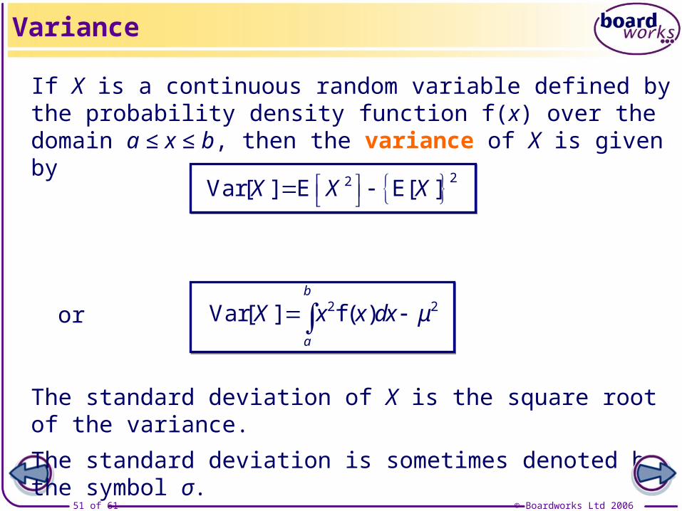
If X is a continuous random variable defined by the probability density function f(x) over the domain a ≤ x ≤ b, then the variance of X is given by
[ ]22Var[ ] E EX X X
or
Variance
[ ] f ( )b
a
X x x dx μ 2 2Var
The standard deviation of X is the square root of the variance.
The standard deviation is sometimes denoted by the symbol σ.
© Boardworks Ltd 200652 of 61
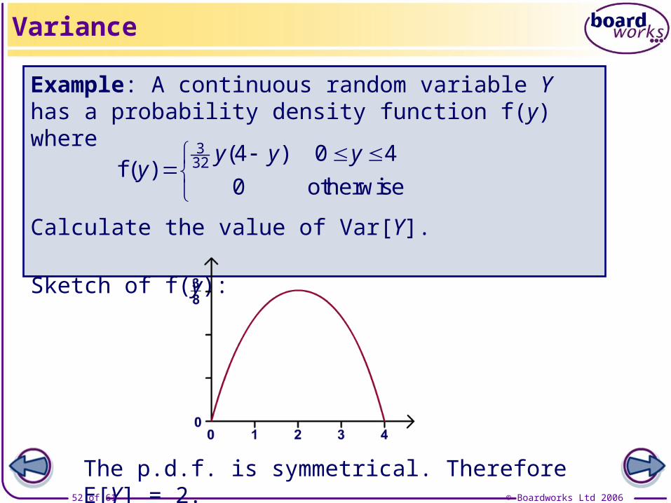
Example: A continuous random variable Y has a probability density function f(y) where
( )f ( )
332 4 0 4
0 otherwise
y y yy
Sketch of f(y):
The p.d.f. is symmetrical. Therefore E[Y] = 2.
Variance
Calculate the value of Var[Y].
© Boardworks Ltd 200653 of 61
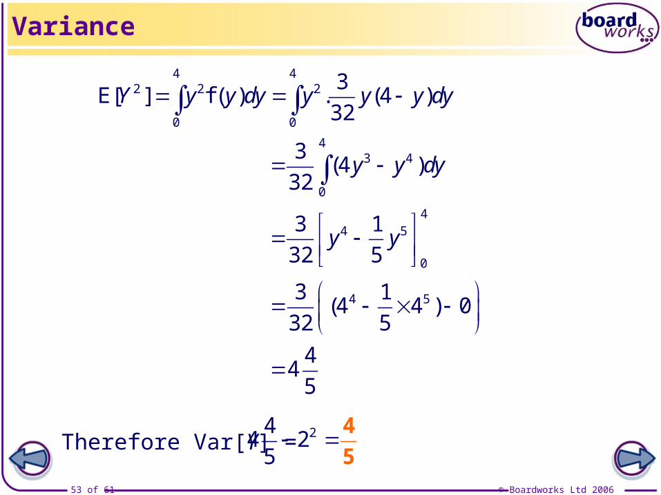
[ ] f ( ) . ( )4 4
2 2 2
0 0
3E 4
32Y y y dy y y y dy
Variance
( )4
3 4
0
34
32y y dy
( )4 53 14 4 0
32 5
44
5
44 5
0
3 1
32 5y y
Therefore Var[Y] = 24
4 25
4
5

© Boardworks Ltd 200654 of 61
Example: A continuous random variable x has a probability density function f(x) where
f ( )
14
38 16
0 2
2 6
0 otherwise
x
x
x x
Calculate
a) the mean value, μ.
b) the standard deviation, σ.
Variance
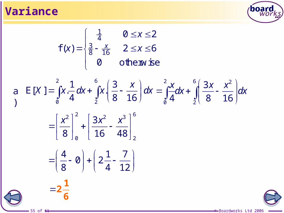
© Boardworks Ltd 200655 of 61
Variance
[ ] . .2 6
0 2
1 3E
4 8 16
xX x dx x dx
2 6 2
0 2
3
4 8 16
x x xdx dx
2 62 2 3
0 2
3
8 16 48
x x x
4 1 70 2
8 4 12
f ( )
14
38 16
0 2
2 6
0 otherwise
x
x
x x
1
26
a)

© Boardworks Ltd 200656 of 61
Variance
[ ] . .2 6
2 2 2
0 2
1 3E
4 8 16
xX x dx x dx
2 62 2 3
0 2
3
4 8 16
x x xdx dx
2 63 3 4
0 212 8 64
x x x
2 3 30 6
3 4 4 , [ ]
22 1 35
So Var 6 2 13 6 36
X
f ( )
14
38 16
0 2
2 6
0 otherwise
x
x
x x
b)
26
3
Therefore σ = 7136 = 1.40 (3 s.f.)
© Boardworks Ltd 200657 of 61
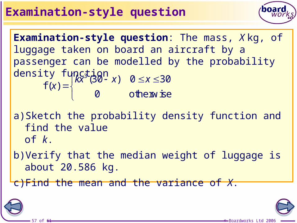
Examination-style question: The mass, X kg, of luggage taken on board an aircraft by a passenger can be modelled by the probability density function
( )f ( )
3 30 0 30
0 otherwise
kx x xx
a) Sketch the probability density function and find the value of k.
b) Verify that the median weight of luggage is about 20.586 kg.
c) Find the mean and the variance of X.
Examination-style question
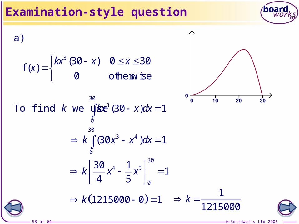
© Boardworks Ltd 200658 of 61
To find k we use ( )30
3
0
30 1kx x dx
Examination-style question
1215000 0 1k 1
1215000k
( )30
3 4
0
30 1k x x dx 30
4 5
0
30 11
4 5k x x
a)
( )f ( )
3 30 0 30
0 otherwise
kx x xx
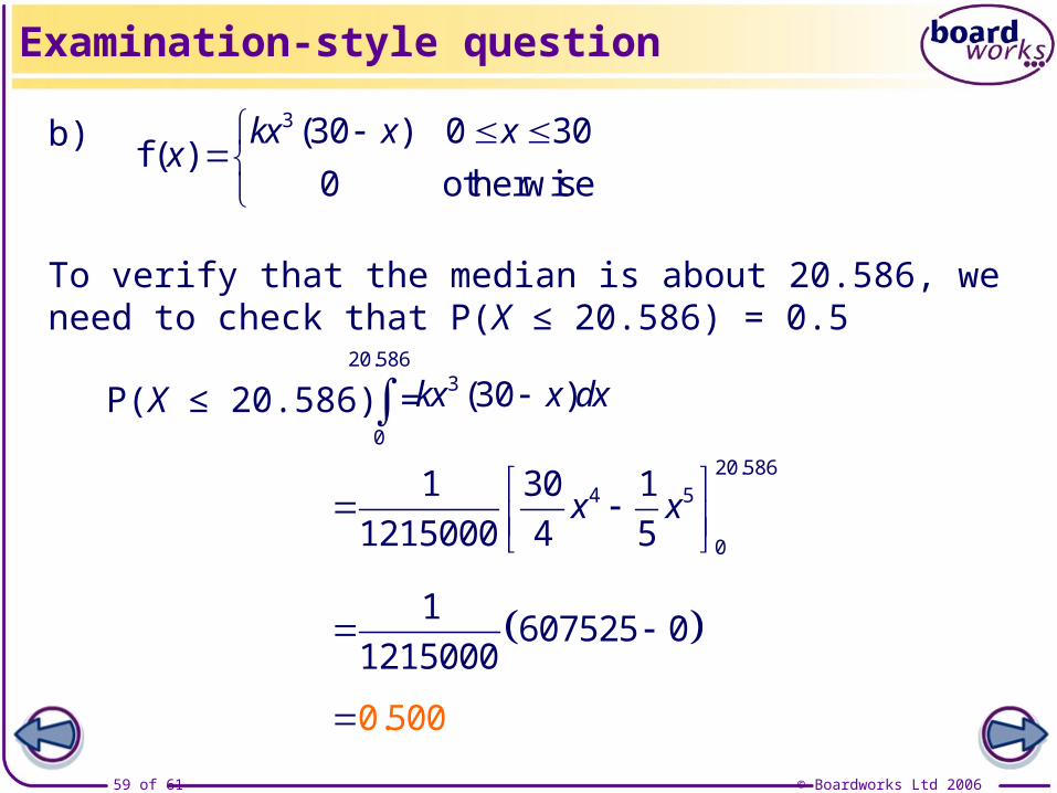
© Boardworks Ltd 200659 of 61
.
( )20 586
3
0
30kx x dx
To verify that the median is about 20.586, we need to check that P(X ≤ 20.586) = 0.5
Examination-style question
1607525 0
1215000
.0 500
.20 5864 5
0
1 30 1
1215000 4 5x x
b) ( )f ( )
3 30 0 30
0 otherwise
kx x xx
P(X ≤ 20.586) =
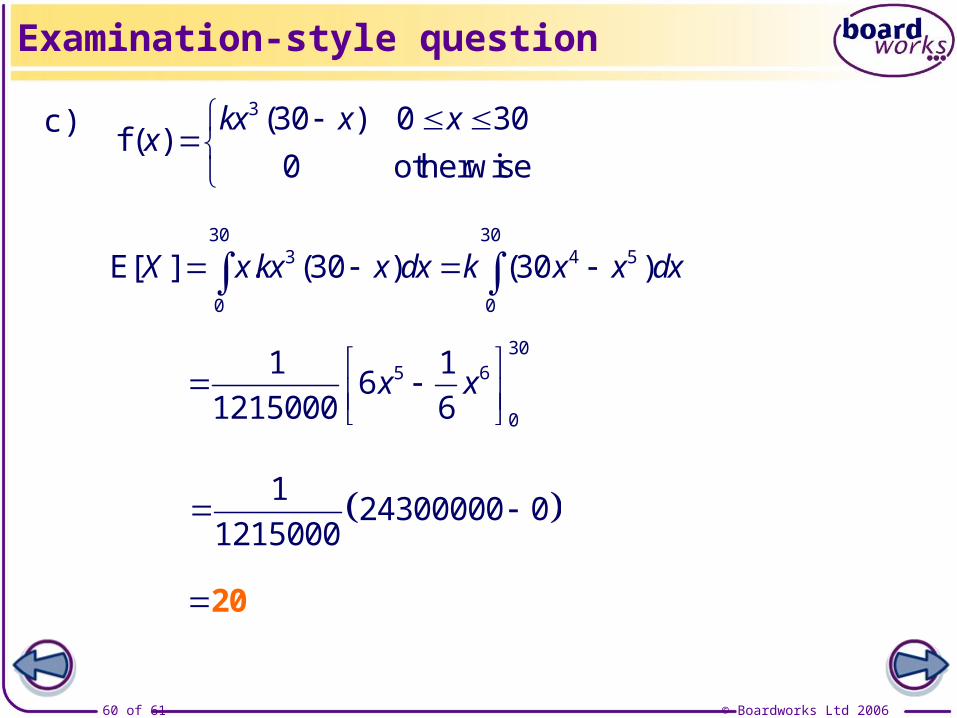
© Boardworks Ltd 200660 of 61
( )f ( )
3 30 0 30
0 otherwise
kx x xx
[ ] . ( ) ( )30 30
3 4 5
0 0
E 30 30X x kx x dx k x x dx
Examination-style question
124300000 0
1215000
20
305 6
0
1 16
1215000 6x x
c)
© Boardworks Ltd 200661 of 61
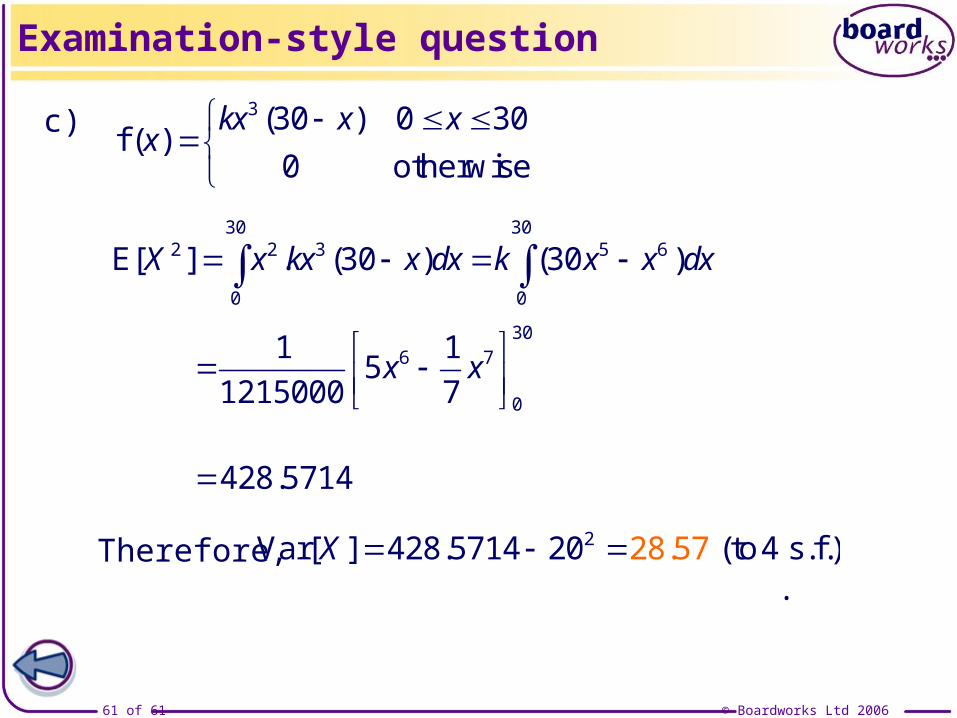
[ ] . ( ) ( )30 30
2 2 3 5 6
0 0
E 30 30X x kx x dx k x x dx
Examination-style question
.428 5714
[ ] . ( ).2Var 428 5714 20 to428 s.f.57X
306 7
0
1 15
1215000 7x x
c)
Therefore, .
( )f ( )
3 30 0 30
0 otherwise
kx x xx
![S2.2 Liguori SouthAfrica2015d284f45nftegze.cloudfront.net/cactusnet/S2.2 Liguori... · 2015. 3. 8. · Title: S2.2 Liguori_SouthAfrica2015 [Compatibility Mode] Author: uvp Created](https://img.dokumen.tips/doc/110x75/60280cba89289271cb7ab913/s22-liguori-southafri-liguori-2015-3-8-title-s22-liguorisouthafrica2015.jpg)