% 3-D vortex-lattice method for a rectangular wingclcclear

% span and chordspan = 10chord = 5

% numbers of rows and columnsnr = 6nc = 12

% angle of attackalpha = 10

% number of steps to be runnsteps = 1

sa = sind(alpha);ca = cosd(alpha);

nrp = nr + 1;ncp = nc + 1;

% grid sizesdy = span/nc;dx = chord/nr;

% grid set-upfor i = 1:nrp

for j = 1:ncpx(i,j) = (i-1)*dx;y(i,j) = (j-1)*dy;z(i,j) = 0;

endend

% coordinates for plottingfor j = 1:ncp

xplt(j) = x(1,j); yplt(j) = y(1,j);

end

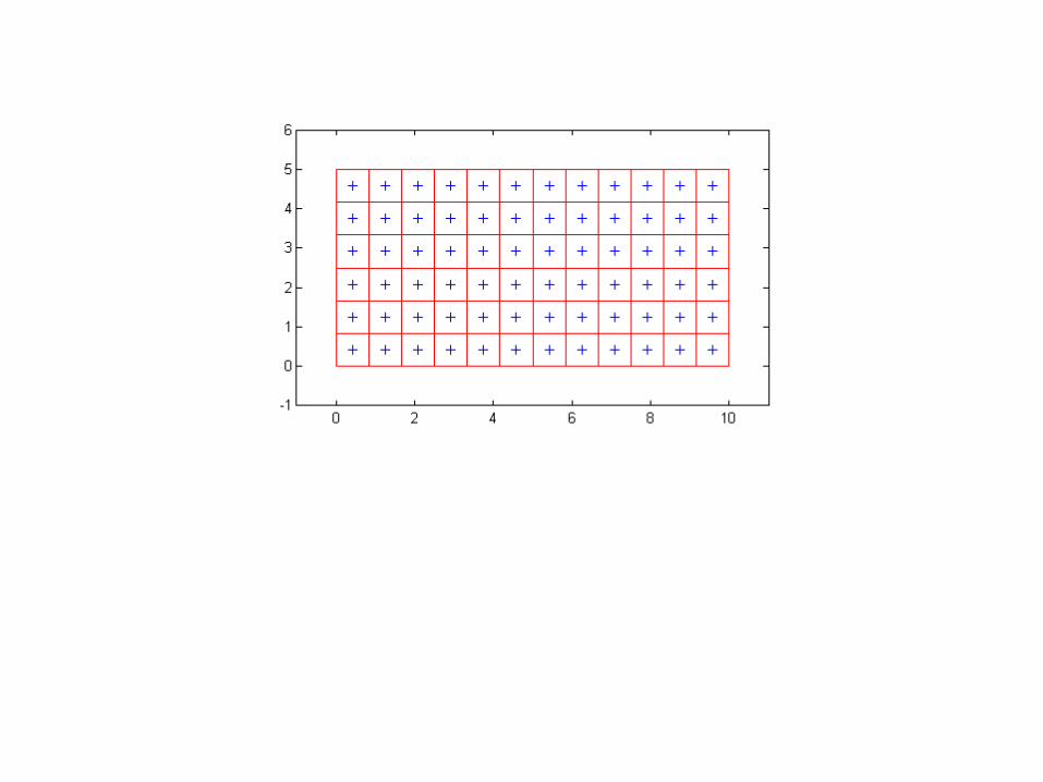
% check the grid% note this figure continues beyond control pointsfigure(1)plot( yplt, xplt,'r' )hold on

for i = 2:nrpfor j = 1:ncp

xplt(j) = x(i,j); yplt(j) = y(i,j);

endplot( yplt, xplt,'r' )

end

for j = 1:ncpfor i = 1:nrp

xplt(i) = x(i,j); yplt(i) = y(i,j);

endplot( yplt, xplt,'r' )

endaxis equal

% number the elements and define the control points% and vectors normal to the elementsn = 0;for i = 1:nr

for j = 1:nc

n = n + 1;

% control points

xcp(n) = 0.25*( x(i,j) + x(i,j+1) + x(i+1,j+1) + x(i+1,j) ); ycp(n) = 0.25*( y(i,j) + y(i,j+1) + y(i+1,j+1) + y(i+1,j) );zcp(n) = 0.25*( z(i,j) + z(i,j+1) + z(i+1,j+1) + z(i+1,j) );

% the normal vectors

d1x = x(i+1,j+1) - x(i,j);d1y = y(i+1,j+1) - y(i,j);d1z = z(i+1,j+1) - z(i,j);

d2x = x(i,j+1) - x(i+1,j);d2y = y(i,j+1) - y(i+1,j);d2z = z(i,j+1) - z(i+1,j);

nx(n) = d1y*d2z - d1z*d2y;ny(n) = d1z*d2x - d1x*d2z;nz(n) = d1x*d2y - d1y*d2x;

endend

% total number of elements: nel = nr*nc; check?nel = n;

% plot control points on gridplot( ycp, xcp,'+b')axis([-1,11, -1, 6])hold off

% influence matrix

for nrec = 1:nel

xp = xcp(nrec);yp = ycp(nrec);zp = zcp(nrec);

for i = 1:nrpfor j = 1:nc

x1 = x(i,j);y1 = y(i,j);z1 = z(i,j);

x2 = x(i,j+1);y2 = y(i,j+1);z2 = z(i,j+1);

[ u, v, w ] = BSL( x1,y1,z1, x2,y2,z2, xp,yp,zp );

s(i,j) = nx(nrec)*u + ny(nrec)*v + nz(nrec)*w;end

end

for i = 1:nrfor j = 1:ncp

x1 = x(i,j);y1 = y(i,j);z1 = z(i,j);

x2 = x(i+1,j);y2 = y(i+1,j);z2 = z(i+1,j);

[ u, v, w ] = BSL_A( x1,y1,z1, x2,y2,z2, xp,yp,zp );

c(i,j) = nx(nrec)*u + ny(nrec)*v + nz(nrec)*w;end

end

nsen = 0;for i = 1:nr

for j = 1:ncnsen = nsen +1;

A(nrec, nsen) = s(i,j) + c(i,j+1) - s(i+1,j) - c(i,j);

endend

end

for n = 1:nelR(n) = -ca*nx(n) - sa*nz(n);

end

G = inv(A)*R';

% circulations around the vortex segments

% spanwise segmentsgs(1:nc) = G(1:nc);

for n = ( nc+1 ):( nr*nc )gs(n) = G(n) - G(n-nc);

end

for n = (nel+1):( nr*(nc+1) )gs(n) = -G(n-nel);

end

% chordwise segmentsn = 0;nch = 0;for i = 1:nr

n = n + 1;nch = nch +1;gc(nch) = G(n);for j = 2:nc

n = n+1;nch = nch+1;gc(nch) = G(n)-G(n-1);

endnch = nch+1;gc(nch) = -G(n);

end

% shed the vorticity along the tips and % trailing edge into the wake

for time = 1:nsteps% starboard wing tip for i = 1:nr

n = (i-1)*nc + 1;xw(i,time) = x( i, 1 );yw(i,time) = y( i, 1 );zw(i,time) = z( i, 1 );Gw(i,time) = G(n);

end

% trailing edgen = (nr-1)*nc + 1;for j = 2:nc-1

n = n + 1;xw(nr-1+j, time) = x(nrp,j);yw(nr-1+j, time) = y(nrp,j);zw(nr-1+j, time) = z(nrp,j);Gw(nr-1+j, time) = G(n);

end

xw(nr+nc-1, time) = x(nrp,nc);yw(nr+nc-1, time) = y(nrp,nc);zw(nr+nc-1, time) = z(nrp,nc);

% port wing tipfor k = 1:nr

n = nr*nc - (k-1)*nc ;xw(nr-1+nc+k, time) = x(nrp-k, ncp);yw(nr-1+nc+k, time) = y(nrp-k, ncp);zw(nr-1+nc+k, time) = z(nrp-k, ncp);Gw(nr-2+nc+k, time) = G(n);

endend

0.608580.221190.092136

-1.1102e-016-0.092136-0.22119-0.60858

0.0615320.0223750.0093231

-3.0655e-018-0.0093231-0.022375-0.061532

Comparison: Center Span 3-D, AR = 6 and 2-D Immediately after an impulsive start, α

= 10o

spanwise circulations

3-D 2-D

spanwise circulations at the wingtip

0.350580.0959840.0355461.6653e-016

-0.035546-0.095984-0.35058

movie: “one”

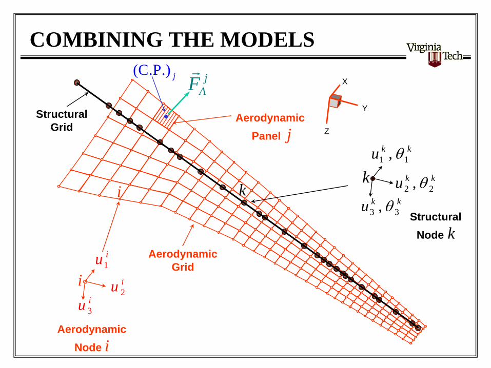
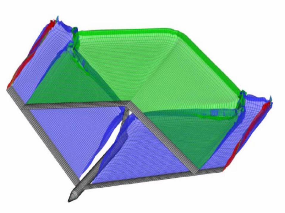
COMBINING THE MODELS(C.P.) j

StructuralGrid

X

Y

Z

i

i

AerodynamicGrid

k

Structural Node k

jAF

Aerodynamic Panel j

k

AerodynamicNode i

1iu

2iu

3iu

1 1,k ku θ

2 2,k ku θ

3 3,k ku θ

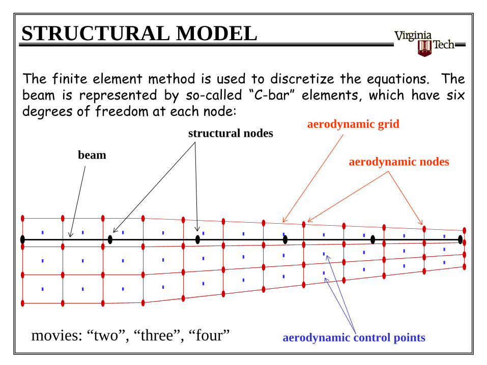
beam

structural nodesaerodynamic grid

aerodynamic nodes

aerodynamic control points

STRUCTURAL MODEL

The finite element method is used to discretize

the equations. The beam is represented by so-called “C-bar”

elements, which have six degrees of freedom at each node:

movies: “two”, “three”, “four”

Time-Domain Nonlinear Aeroelastic Analysis with Discrete-Gust Excitation:

A HALE-Wing Case Study

Z. WangP. C. ChenD. D. Liu

D. T. MookM. J. Patil

movie: “five”

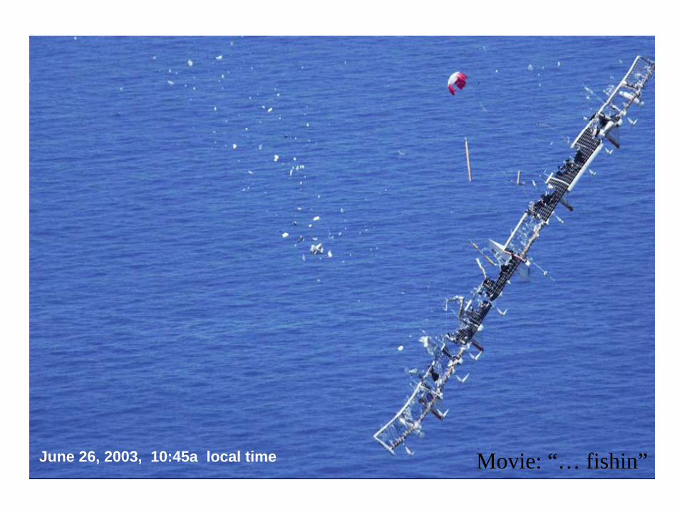
June 26, 2003, 10:45a local time Movie: “… fishin”