Embed Size (px)
Citation preview

© 2014 Zvi M. Kedem 1
Unit 8Physical Design
And Query Execution Concepts

© 2014 Zvi M. Kedem 2
Physical Design in Context
Base TablesConstraints, Privileges
Base TablesConstraints, Privileges
FilesIndexes, Distribution
FilesIndexes, Distribution
Standard OSStandard Hardware
Standard OSStandard Hardware
ConcurrencyConcurrency
RecoveryRecovery
Derived TablesConstraints, Privileges
Derived TablesConstraints, Privileges
DerivedDerived
ImplementedImplemented
Relies onRelies on
Runs onRuns on
Application Data Analysis (ER)Application Data Analysis (ER)
Normalization (NFs)Normalization (NFs)
Transaction Processing (ACID, Sharding)Transaction Processing (ACID, Sharding)
Queries (DML)Queries (DML)
User Level(View Level)User Level
(View Level)
Community Level(Base Level)
Community Level(Base Level)
Physical LevelPhysical Level
DBMS OS LevelDBMS OS Level
CentralizedOr
Distributed
CentralizedOr
Distributed
Queries (DML)Queries (DML)
Schema Specification (DDL)Schema Specification (DDL)
Query Execution (B+, …, Execution Plan)Query Execution (B+, …, Execution Plan)

© 2014 Zvi M. Kedem 3
Database Design
Logical DB Design:1. Create a model of the enterprise (e.g., using ER)2. Create a logical “implementation” (using a relational model and
normalization)· Creates the top two layers: “User” and “Community”· Independent of any physical implementation
Physical DB Design· Uses a file system to store the relations· Requires knowledge of hardware and operating system’s
characteristics· Addresses questions of distribution (distributed databases), if
applicable· Creates the third layer
Query execution planning and optimization ties the two together; not the focus of this unit, but some issues discussed

© 2014 Zvi M. Kedem 4
Physical Design

© 2014 Zvi M. Kedem 5
Issues Addressed In Physical Design
The new aspect: the database in general does not fit in RAM, so need to manage carefully access to disks
Main issues addressed generally in physical design· Storage Media· File structures· Indexes
We concentrate on· Centralized (not distributed) databases· Database stored on a disk using a “standard” file system, not one
“tailored” to the database· Database using unmodified general-purpose operating system· Indexes
The only criterion we consider in this unit is performance

© 2014 Zvi M. Kedem 6
What is a Disk?
Illustrations from Wikipedia, in public domain A disk is a “stack” of platters A cylinder is a stack of tracks denoted by letter “A” on our
one platter, in which it is only a ring Our typical block (next slide) is the red segment denoted
by letter “C”
A
BC
D

© 2014 Zvi M. Kedem 7
What Is A Disk?
Disk consists of a sequence of cylinders A cylinder consists of a sequence of tracks A track consist of a sequence of sectors A sector contains
· Data area· Header· Error-correcting information
We only care about the data area and will refer to it as a block
For us: A disk consists of a sequence of blocks All blocks are of same size, say 512 B or 4 096 B (bytes) 512 bytes is rather small but it is a very long-standing
standard and many legacy programs rely on this size We assume: a virtual memory page is the same size a
block
© 2014 Zvi M. Kedem 8
What Is A Disk?
A physical unit of access is always a block. If an application wants to read one or more bits that are in
a single block · If an up-to-date copy of the block is in RAM already (as a page in
virtual memory), read from the page· If not, the system reads a whole block and puts it as a whole page
in a disk cache in RAM

© 2014 Zvi M. Kedem 9
What Is A File?
File can be thought of as “logical” or a “physical” entity
File as a logical entity: a sequence of records Records are either fixed size or variable size
A file as a physical entity: a sequence of fixed size blocks (on the disk), but not necessarily physically contiguous (the blocks could be dispersed)
Blocks in a file are either physically contiguous or not, but the following is generally simple to do (for the file system):· Find the first block· Find the last block· Find the next block· Find the previous block

© 2014 Zvi M. Kedem 10
What Is A File?
Records are stored in blocks· This gives the mapping between a “logical” file and a “physical”
file
Assumptions (some to simplify presentation for now)· Fixed size records· No record spans more than one block· There are, in general, several records in a block· There is some “left over” space in a block as needed later (e.g.,
for chaining the blocks of the file)
We assume that each relation is stored as a file Each tuple is a record in the file

© 2014 Zvi M. Kedem 11
Example: Storing A Relation (Logical File)
1 1200
3 2100
4 1800
2 1200
6 2300
9 1400
8 1900
E# Salary1 12003 21004 18002 12006 23009 14008 1900
RecordsRelation

© 2014 Zvi M. Kedem 12
Example: Storing A Relation (Physical File)
Blocks
1 1200
3 2100
4 1800
2 1200
6 2300
9 1400
8 1900
Records
6 23009 1400
1 1200 3 2100 8 1900
4 18002 1200
Left-overSpaceFirst block
of the file

© 2014 Zvi M. Kedem 13
Processing A Query
Simple query
SELECT E#FROM RWHERE SALARY > 1500;
What needs to be done “under the hood” by the file system:· Read into RAM at least all the blocks containing all records
satisfying the condition (assuming none are in RAM.– It may be necessary/useful to read other blocks too, as we see later
· Get the relevant information from the blocks· Perform additional processing to produce the answer to the query
What is the cost of this? We need a “cost model”

© 2014 Zvi M. Kedem 14
Cost Model
Two-level storage hierarchy· RAM· Disk (and more and more Solid State Drive (SSD))
Reading or Writing a block costs one time unit Processing in RAM is free Ignore caching of blocks (unless done previously by the
query itself, as the byproduct of reading) Justifying the assumptions
· Accessing the disk is much more expensive than any reasonable CPU processing of queries (we could be more precise, which we are not here)
· We do not want to account formally for block contiguity on the disk; we do not know how to do it well in general (and in fact what the OS thinks is contiguous may not be so: the disk controller can override what OS thinks)
· We do not want to account for a query using cache slots “filled” by another query; we do not know how to do it well, as we do not know in which order queries come

© 2014 Zvi M. Kedem 15
Implications of the Cost Model
Goal: Minimize the number of block accesses
A good heuristic: Organize the physical database so that you make as much use as possible from any block you read/write
Note the difference between the cost models in· Data structures (where “analysis of algorithms” type of cost model
is used: minimize CPU processing)· Data bases (minimize disk accessing)
There are serious implications to this difference
Database physical (disk) design is obtained by extending and “fine-tuning” of “classical” data structures
© 2014 Zvi M. Kedem 16
Example
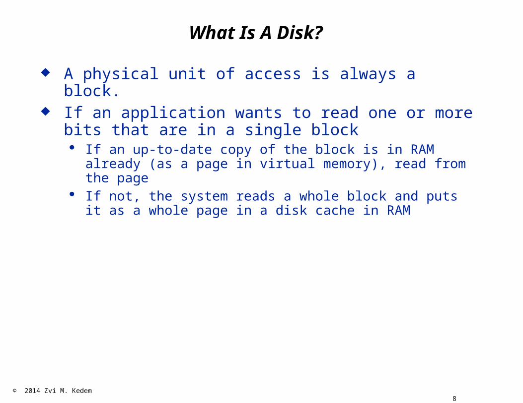
If you know exactly where E# = 2 and E# = 9 are:
The data structure cost model gives a cost of 2 (2 RAM accesses)
The database cost model gives a cost of 2 (2 block accesses)
Blocks on disk
1 12003 2100
4 18002 1200
6 23009 14008 1900
Array in RAM
6 23009 1400
1 1200 3 2100 8 1900
4 18002 1200

© 2014 Zvi M. Kedem 17
Example
If you know exactly where E# = 2 and E# = 4 are:
The data structure cost model gives a cost of 2 (2 RAM accesses)
The database cost model gives a cost of 1 (1 block access)
Blocks on disk
1 12003 2100
4 18002 1200
6 23009 14008 1900
Array in RAM
6 23009 1400
1 1200 3 2100 8 1900
4 18002 1200

© 2014 Zvi M. Kedem 18
File Organization and Indexes
If we know what we will generally be reading/writing, we can try to minimize the number of block accesses for “frequent” queries
Tools:· File organization· Indexes (structures showing where records are located)
Essentially: File organization tries to provide:· When you read a block you get “many” useful records
Essentially: Indexes try to provide:· You know where blocks containing useful records are
We discuss both in this unit

© 2014 Zvi M. Kedem 19
Tradeoff
Maintaining file organization and indexes is not free Changing (deleting, inserting, updating) the database
requires · Maintaining the file organization · Updating the indexes
Extreme case: database is used only for SELECT queries· The “better” file organization is and the more indexes we have will
result in more efficient query processing
Extreme case: database is used only for INSERT queries· The simpler file organization and no indexes will result in more
efficient query processing· Perhaps just append new records to the end of the file
In general, somewhere in between

© 2014 Zvi M. Kedem 20
Review Of Data Structures To Store N Numbers
Heap: unsorted sequence (note difference from a common use of the term “heap” in data structures)
Sorted sequence
Hashing
2-3 trees

© 2014 Zvi M. Kedem 21
Heap (Assume Contiguous Storage)
Finding (including detecting of non-membership)Takes between 1 and N operations
DeletingTakes between 1 and N operations
Depends on the variant also · If the heap needs to be “compacted” it will take always N (first to
reach the record, then to move the “tail” to close the gap)· If a “null” value can be put instead of a “real” value, then it will
cause the heap to grow unnecessarily
InsertingTakes 1 (put in front), or N (put in back if you cannot access the back easily, otherwise also 1), or maybe in between by reusing null values
Linked list: obvious modifications

© 2014 Zvi M. Kedem 22
Sorted Sequence
Finding (including detecting of non-membership)
log N using binary search. But note that “optimized” deletions and insertions could cause this to grow (next transparency)
Deleting
Takes between log N and log N + N operations. Find the integer, remove and compact the sequence.
Depends on the variant also. For instance, if a “null” value can be put instead of a “real” value, then it will cause the sequence to grow unnecessarily.

© 2014 Zvi M. Kedem 23
Sorted Sequence
Inserting
Takes between log N and log N + N operations. Find the place, insert the integer, and push the tail of the sequence.
Depends on the variant also. For instance, if “overflow” values can be put in the middle by means of a linked list, then this causes the “binary search to be unbalanced, resulting in possibly up to N operations for a Find.

© 2014 Zvi M. Kedem 24
Sorted Sequences
We have a sorted sequence of 15, 25, 35, 45, 55, and room for a pointer
26, 27, 28, 29, 30 arrive and are inserted as “overflow” in the right place
It takes a long time to find 30
15 25 35 45 55
15 25 35 45 55
26
27
28
30
29

© 2014 Zvi M. Kedem 25
Hashing
Pick a number B “somewhat” bigger than N
Pick a “good” pseudo-random function hh: integers ® {0,1, ..., B – 1}
Create a “bucket directory,” D, a vector of length B, indexed 0,1, ..., B – 1
For each integer k, it will be stored in a location pointed at from location D[h(k)], or if there are more than one such integer to a location D[h(k)], create a linked list of locations “hanging” from this D[h(k)]
Probabilistically, almost always, most of the locations D[h(k)], will be pointing at a linked list of length 1 only

© 2014 Zvi M. Kedem 26
Hashing: Example Of Insertion
N = 7
B = 10
h(k) = k mod B (this is an extremely bad h, but good for a simple example)
Integers arriving in order:
37, 55, 21, 47, 35, 27, 14

© 2014 Zvi M. Kedem 27
Hashing: Example Of Insertion
0
1
2
345
6
7
8
9
37
55
0
1
2
345
6
7
8
9
37
0
1
2
345
6
7
8
9
37
55
21
0
1
2
345
6
7
8
9

© 2014 Zvi M. Kedem 28
Hashing: Example Of Insertion
47
37
55
21
0
1
2
345
6
7
8
9
35
47
37
55
21
0
1
2
345
6
7
8
9

© 2014 Zvi M. Kedem 29
Hashing: Example Of Insertion
47
37
55
21
0
1
2
345
6
7
8
9
35
27
14
47
37
55
21
0
1
2
345
6
7
8
9
35
27

© 2014 Zvi M. Kedem 30
Hashing
Assume, computing h is “free”
Finding (including detecting of non-membership)Takes between 1 and N + 1 operations.
Worst case, there is a single linked list of all the integers from a single bucket.
Average, between 1 (look at bucket, find nothing) and a little more than 2 (look at bucket, go to the first element on the list, with very low probability, continue beyond the first element)

© 2014 Zvi M. Kedem 31
Hashing
Inserting
Obvious modifications of ”Finding”
But sometimes N is “too close” to B (bucket table becomes too small)· Then, increase the size of the bucket table and rehash· Number of operations linear in N· Can amortize across all accesses (ignore, if you do not know what
this means)
Deleting
Obvious modification of “Finding”
Sometimes bucket table becomes too large, act “opposite” to Inserting

© 2014 Zvi M. Kedem 32
2-3 Tree (Example)
2 4 7 10 11 18 20 30 32 40 45 57 59 61 75 77 78 82 87
20 57
7 11 32 61 78

© 2014 Zvi M. Kedem 33
2-3 Trees
A 2-3 tree is a rooted (it has a root) directed (order of children matters) tree
All paths from root to leaves are of same length Each node (other than leaves) has between 2 and 3
children For each child of a node, other than the last, there is an
index value stored in the node For each non-leaf node, the index value indicates the
largest value of the leaf in the subtree rooted at the left of the index value.
A leaf has between 2 and 3 values from among the integers to be stored

© 2014 Zvi M. Kedem 34
2-3 Trees
It is possible to maintain the “structural characteristics above,” while inserting and deleting integers
Sometimes for insertion or deletion of integers there is no need to insert or delete a node· E.g., inserting 19· E.g., deleting 45
Sometimes for insertion or deletion of integers it is necessary to insert or delete nodes (and thus restructure the tree)· E.g., inserting 88,89,97· E.g., deleting 40, 45
Each such restructuring operation takes time at most linear in the number of levels of the tree (which, if there are N leaves, is between log3N and log2N; so we write: O(log N) )
We show by example of an insertion

© 2014 Zvi M. Kedem 35
Insertion Of A Node In The Right Place
First example: Insertion resolved at the lowest level

© 2014 Zvi M. Kedem 36
Insertion Of A Node In The Right Place
Second example: Insertion propagates up to the creation of a new root

© 2014 Zvi M. Kedem 37
2-3 Trees
Finding (including detecting of non-membership)
Takes O(log N) operations
Inserting while keeping trees balanced
Takes O(log N) operations
Deleting while keeping trees balanced
Takes O(log N) operations. We do not show this as it is more complicated and sometimes balancing is not considered while doing deletions

© 2014 Zvi M. Kedem 38
What To Use?
If the set of integers is large, use either hashing or 2-3 trees
Use 2-3 trees if “many” of your queries are range queries Find all the SSNs (integers) in your set that lie in the
range 070430000 to 070439999 Use hashing if “many” of your queries are not range
queries If you have a total of 10,000 integers randomly chosen
from the set 0 ,..., 999999999, how many will fall in the range above?
How will you find the answer using hashing, and how will you find the answer using 2-3 trees?

© 2014 Zvi M. Kedem 39
Back To Databases
We have a file of blocks· Each block is a sequence of records
Whenever we read or write, we read or write a block: no smaller unit is physically accessible
We had two “principles”
Organize the file so that when you read a block you get “many” useful records
Organize an index to a file so that you easily find the useful blocks

© 2014 Zvi M. Kedem 40
Index And File
In general, we have a data file of blocks, with blocks containing records
Each record has a field, which contains a key, uniquely labeling/identifying the record and the “rest” of the record
There is an index, which is another file which essentially (we will be more precise later) consists of records which are pairs of the form (key, block address)
For each (key, block address) pair (K, B) in the index file, the block address contains a pointer to a block of the file that contains the record with that key
But we are not saying that necessarily for every record in the file with key = K in block address B there is an there is a pair (K, B) in the index file

© 2014 Zvi M. Kedem 41
Reminder On Data Structures
The index is a binary search tree The file is just a set of numbers not organized in any
particular way: e.g., the numbers do not have to be contiguous
Index
File

© 2014 Zvi M. Kedem 42
Reviewing Binary Search Trees In Data Structures
Each node of the index consists of · A pointer to the root of the left subtree· A pointer to the root of the right subtree· A separator (number)
All the leaves of the left subtree are smaller that all the leaves of the right subtree
The separator is the largest leaf in the left subtree It is clear how to search for a number: the separator tells
you into which subtree to go
2 874
Index
Set of Numbers
4
2 7

© 2014 Zvi M. Kedem 43
Binary Search Trees In Databases
In databases (on a disk) we have as leaves blocks that in general contain several records.
Each record has a field, which is the key for that record All the keys are different
· Think: record in a file = tuple in a table· Think: key field of a file = primary key of a table
x
subtreewhose
leaves containrelevant records
with keysless or equal to x
subtreewhose
leaves containrelevant records
with keysgreater than x
A node of the index (root or internal)

© 2014 Zvi M. Kedem 44
Index: Dense or Sparse
An index is dense if for every record (that is for every key value) that we have in the database there is a pointer from the index to the block containing the record (in our example a block contains two records and we only show the key values in the records)· Pointers always point at blocks and not at records· Once a block is in RAM, useful records are easily found
Otherwise, an index is sparse
2 8 7 4 8 7 2 4
4
72 4
dense index and unclustered file sparse index and clustered file

© 2014 Zvi M. Kedem 45
File: Clustered or Unclustered
A file is clustered if it can be “fully” sorted without moving records between blocks
We can only move blocks around and records inside block Otherwise, a file is unclustered In our example, the second file is clustered because it can
be sorted like this
2 8 7 4 8 7 2 4
4
72 4
dense index and unclustered file sparse index and clustered file
872 4

© 2014 Zvi M. Kedem 46
Best: Clustered File + Sparse Index
Clustered file implies that a block has “related” records Sparse index implies that it is efficient to find a block
containing “interesting” records
Below, on the right, all records with key greater than 4 are in one block
Below, on the right, the index has only 1 level so only 1 block of the index is read to know the block of interest
2 8 7 4 8 7 2 4
4
72 4
dense index and unclustered file sparse index and clustered file

© 2014 Zvi M. Kedem 47
2-3 Trees Revisited
We again consider a file of records of interest Each record has one field, which serves as primary key,
which will be an integer 2 records can fit in a block Sometimes a block will contain only 1 record We will consider 2-3 trees as indexes pointing at the
records of this file
The file contains records with indexes: 1, 3, 5, 7, 9

© 2014 Zvi M. Kedem 48
Dense Index And Unclustered File
Pointers point from the leaf level of the tree to blocks (not records) of the file· Multiple pointers point at a block
For each value of the key there is a pointer for such value· Sometimes the value of the key in index is explicit, such as 1· Sometimes the value of the key in index is implicit, such as 5
(there is one value between 3 and 7 and the pointer is the 3rd pointer coming out from the leftmost leaf and it points to a block which contains the record with the key value of 5
5
1 3 7
9 1 3 7 5

© 2014 Zvi M. Kedem 49
Sparse Index And Clustered File
Pointers point from the leaf level of the tree to blocks (not records) of the file· A single pointer points at a block
For each value of the key that is the largest in a block there is a pointer for such value· Sometimes the key value is explicit, such as 3· Sometimes the key value is implicit, such as 5
Because of clustering we know where 1 is
5
3 7
1 3 5 97
© 2014 Zvi M. Kedem 50
To Summarize The“Quality” Of Choices In General
Sparse index and unclustered file: generally bad, cannot easily find records for some keys
Dense index and clustered file: generally unnecessarily large index (we will learn later why)
Dense index and unclustered file: good, can easily find the record for every key
Sparse index and clustered file: best (we will learn later why)

© 2014 Zvi M. Kedem 51
Search Trees
We will study in greater depth search tree for finding records in a file
They will be a generalization of 2-3 trees For very small files, the whole tree could be just the root
· For example, in the case of 2-3 trees, a file of 1 record, for instance
So to make the presentation simple, we will assume that there is at least one level in the tree below the root· The case of the tree having only the root is very simple and can
be ignored here

© 2014 Zvi M. Kedem 52
B+-Trees: Generalization Of 2-3 Trees
A B+-tree is a tree satisfying the conditions· It is rooted (it has a root)· It is directed (order of children matters) · All paths from root to leaves are of same length· For some parameter m:
– All internal (not root and not leaves) nodes have between ceiling of m/2 and m children
– The root between 2 and m children
We cannot, in general, avoid the case of the root having only 2 children, we will see soon why

© 2014 Zvi M. Kedem 53
B+-Trees: Generalization Of 2-3 Trees
Each node consists of a sequence (P is address or pointer, I is index or key):P1,I1,P2,I2,...,Pm-1,Im-1,Pm
Ij’s form an increasing sequence. Ij is the largest key value in the leaves in the subtree
pointed by Pj
· Note, others may have slightly different conventions

© 2014 Zvi M. Kedem 54
ExampleDense Index & Unclustered File
m = 57 Although 57 pointers are drawn, in fact between 29 and
57 pointers come out of each non-root node
Leaf N ode
Interna l N ode . . . . . .P1 I1 P56 I56 P57
. . . . . .P1 I1 P56 I56 P57
File B lock Contain ing Record w ith Index I1
F ile B lock Contain ing Record w ith Index I57
F ile B lock Contain ing Record w ith Index I2
(note that I57 is not lis ted in the index file)
Left-overSpace

© 2014 Zvi M. Kedem 55
B+-trees: Properties
Note that a 2-3 tree is a B+-tree with m = 3 Important properties
· For any value of N, and m 3, there is always a B+-tree storing N pointers (and associated key values as needed) in the leaves
· It is possible to maintain the above property for the given m, while inserting and deleting items in the leaves (thus increasing and decreasing N)
· Each such operation only O(depth of the tree) nodes need to be manipulated.
When inserting a pointer at the leaf level, restructuring of the tree may propagate upwards
At the worst, the root needs to be split into 2 nodes The new root above will only have 2 children

© 2014 Zvi M. Kedem 56
B+-trees: Properties
Depth of the tree is “logarithmic” in the number of items in the leaves
In fact, this is logarithm to the base at least ceiling of m/2 (ignore the children of the root; if there are few, the height may increase by 1)
What value of m is best in RAM (assuming RAM cost model)?
m = 3 Why? Think of the extreme case where N is large and m =
N· You get a sorted sequence, which is not good (insertion is
extremely expensive
“Intermediate” cases between 3 and N are better than N but not as good as 3
But on disk the situation is very different, as we will see

© 2014 Zvi M. Kedem 57
An Example
Our application:· Disk of 16 GiB (GiB or gibibyte means 230 bytes, GB or gigabyte
means 109 bytes); very small, but a good example· Each block of 512 bytes; rather small, but a good example· File of 20 000 000 records· Each record of 25 bytes· Each record of 3 fields:
SSN: 5 bytes (packed decimal), name 14 bytes, salary 6 bytes
We want to access the records using the value of SSN We want to use a B+-tree index for this Our goal, to minimize the number of block accesses, so
we want to derive as much benefit from each block So, each node should be as big as possible (have
many pointers), while still fitting in a single block· Traversing a block once it is in the RAM is free
Let’s compute the optimal value of m

© 2014 Zvi M. Kedem 58
An Example:If We Can Do Our Own Design Of B+ Trees
There are 234 bytes on the disk, and each block holds 29 = 512 bytes.
Therefore, there are 234 / 29 = 225 blocks, say numbered 0,1,…,225 – 1; each such number can be stored in 25 bits
Therefore, a block address can be specified in 25 bits; in practice likely determined by the operating system, e.g., 32 or 64 bits,
We will not not rely on what the operating system may do and we will optimize ourselves
That is what you should also do during the course, following what we will do next

© 2014 Zvi M. Kedem 59
An Example:If We Can Do Our Own Design Of B+ Trees
We need 25 bits to store a block address We will allocate 4 bytes to a block address by rounding up
25/8 = 3.125· We may be “wasting” space, by working on a byte as opposed to
a bit level, but simplifying the calculations· It is just a coincidence that this is what a 32-bit operating system
may do
A node in the B-tree will contain some m pointers (each storing a block address) and m – 1 keys, so what is the largest possible value for m, so a node fits in a block?
(m) ´ (size of pointer) + (m – 1) ´ (size of key) £ size of the block(m) ´ (4) + (m – 1) ´ (5) £ 5129m £ 517; m £ 57.4...m has to be an integer and therefore m = 57
© 2014 Zvi M. Kedem 60
An Example
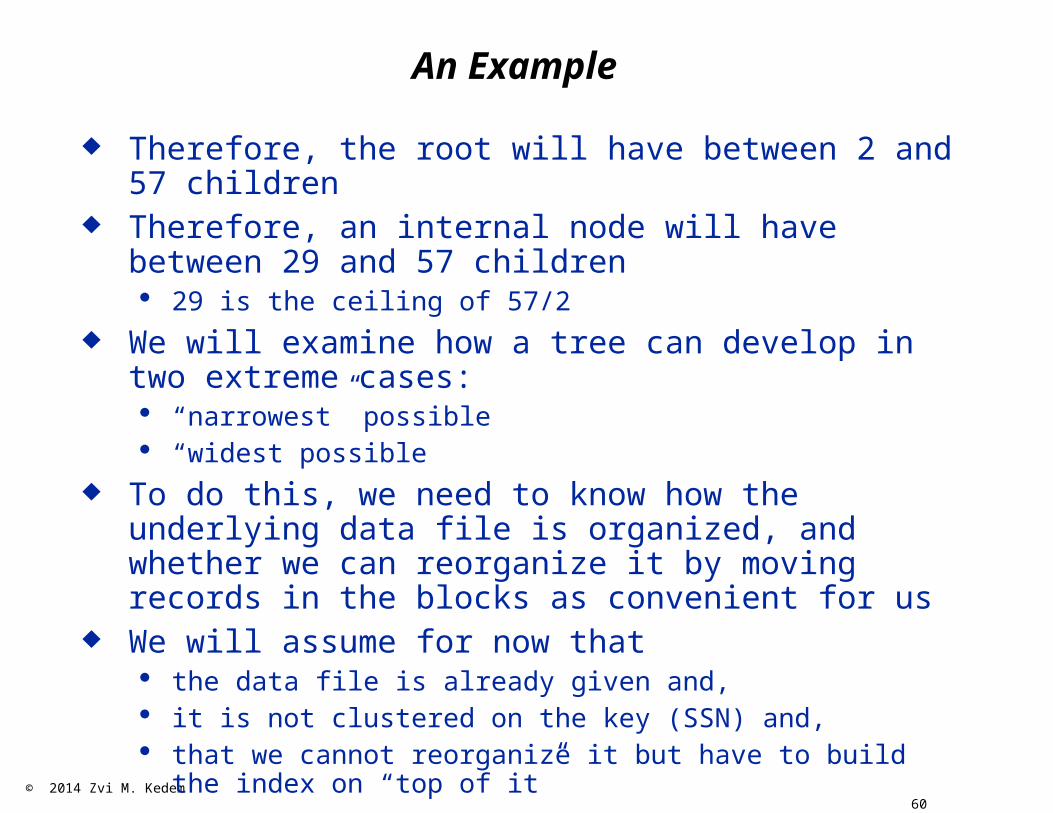
Therefore, the root will have between 2 and 57 children Therefore, an internal node will have between 29 and 57
children· 29 is the ceiling of 57/2
We will examine how a tree can develop in two extreme cases:· “narrowest” possible· “widest possible
To do this, we need to know how the underlying data file is organized, and whether we can reorganize it by moving records in the blocks as convenient for us
We will assume for now that· the data file is already given and,· it is not clustered on the key (SSN) and,· that we cannot reorganize it but have to build the index on “top of
it”

© 2014 Zvi M. Kedem 61
ExampleDense Index And Unclustered File
In fact, between 2 and 57 pointers come out of the root In fact, between 29 and 57 pointers come out of a non-
root node (internal or leaf)
Leaf N ode
Interna l N ode . . . . . .P1 I1 P56 I56 P57
. . . . . .P1 I1 P56 I56 P57
File B lock Contain ing Record w ith Index I1
F ile B lock Contain ing Record w ith Index I57
F ile B lock Contain ing Record w ith Index I2
(note that I57 is not lis ted in the index file)
Left-overSpace

© 2014 Zvi M. Kedem 62
An Example
We obtained a dense index, where there is a pointer “coming out” of the index file for every existing key in the data file
Therefore we needed a pointer “coming out” of the leaf level for every existing key in the data file, that is for every record
We must get a total of 20 000 000 pointers “coming out” in the lowest level
In the narrow tree, other than at the root, every node has 29 pointers “coming out of it” (29 children)
In the narrow tree, the root has 2 pointers “coming out of it” (2 children)
In the wide tree, every node has 57 pointers coming out of it (57 children)
© 2014 Zvi M. Kedem 63
An Example
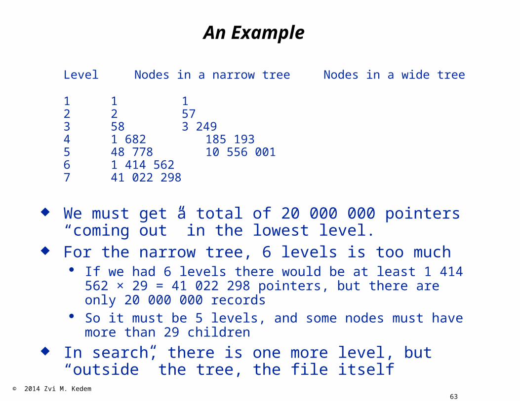
Level Nodes in a narrow tree Nodes in a wide tree
1 1 12 2 573 58 3 2494 1 682 185 1935 48 778 10 556 0016 1 414 5627 41 022 298
We must get a total of 20 000 000 pointers “coming out” in the lowest level.
For the narrow tree, 6 levels is too much · If we had 6 levels there would be at least 1 414 562 × 29 =
41 022 298 pointers, but there are only 20 000 000 records· So it must be 5 levels, and some nodes must have more than 29
children
In search, there is one more level, but “outside” the tree, the file itself

© 2014 Zvi M. Kedem 64
An Example
Level Nodes in a narrow tree Nodes in a wide tree
1 1 12 2 573 58 3 2494 1 682 185 1935 48 778 10 556 0016 1 414 5627 41 022 298
For the wide tree, 4 levels is too little· If we had 4 levels there would be at most 185 193 × 57 =
10 556 001 pointers, but there are 20 000 000 records· So it must be 5 levels
Not for the wide tree we round up the number of levels Conclusion: it will be 5 levels exactly in the tree (accident
of the example; in general could be some range) In search, there is one more level, but “outside” the tree,
the file itself

© 2014 Zvi M. Kedem 65
An Example
How does B+ compare with a sorted file? If a file is sorted, it fits in at least 20 000 000 / 20 =
1 000 000 blocks, therefore:
Binary search will take ceiling of log2(1 000 000) = 20 block accesses
As the narrow tree had 5 levels, we needed at most 6 block accesses (5 for the tree, 1 for the file)· We say “at most” as in general there is a difference in
the number of levels between a narrow and a wide tree, so it is not the case of our example in which we could say “we needed exactly 6 block accesses”
· But if the page/block size is larger, this will be even better
A 2-3 tree, better than sorting but not by much

© 2014 Zvi M. Kedem 66
Finding 10 Records
So how many block accesses are needed for reading, say 10 records?
If the 10 records are “random,” then we need possibly close to 60 block accesses to get them, 6 accesses per record· In fact, somewhat less, as likely the top levels of the B-tree are
cashed and therefore no need to read them again for each search of one of the 10 records of interest
Even if the 10 records are consecutive, then as the file is not clustered, they will still (likely be) in 10 different blocks of the file, but “pointed from” 1 or 2 leaf nodes of the tree· We do not know exactly how much we need to spend traversing
the index, worst case to access 2 leaves we may have 2 completely disjoint paths starting from the root, but this is unlikely
· In addition, maybe the index leaf blocks are chained so it is easy to go from a leaf to the following leaf
· So in this case, seems like 16 or 17 block accesses in most cases
© 2014 Zvi M. Kedem 67
An Example
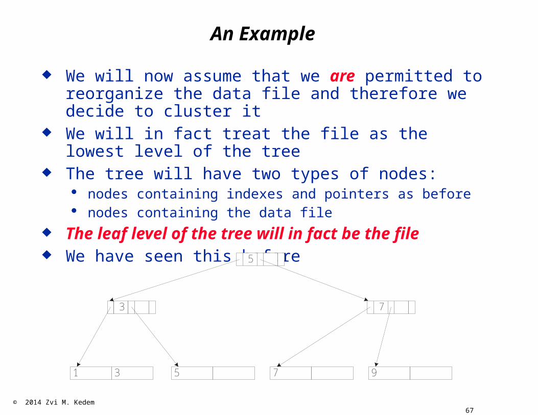
We will now assume that we are permitted to reorganize the data file and therefore we decide to cluster it
We will in fact treat the file as the lowest level of the tree The tree will have two types of nodes:
· nodes containing indexes and pointers as before· nodes containing the data file
The leaf level of the tree will in fact be the file We have seen this before
5
3 7
1 3 5 97

© 2014 Zvi M. Kedem 68
An Example
For our example, at most 20 records fit in a block Each block of the file will contain between 10 and 20
records So the bottom level is just like any node in a B-tree, but
because the “items” are bigger, the value of m is different, it is m = 20
So when we insert a record in the right block, there may be now 21 records in a block and we need to split a block into 2 blocks· This may propagate up
Similarly for deletion We will examine how a tree can develop in two extreme
cases:· “narrowest” possible· “widest possible

© 2014 Zvi M. Kedem 69
An Example
Internal Node
Left-overSpace
Leaf Node
. . . . . .P1 I1 P56 I56 P57
. . .I.. I... rest of rec.rest of rec.
Left-overSpace
For each leaf node (that is a block of the file), there is a pointer associated with the largest key value from the key values appearing in the block; the pointer points from the level just above the leaf of the structure
© 2014 Zvi M. Kedem 70
An Example
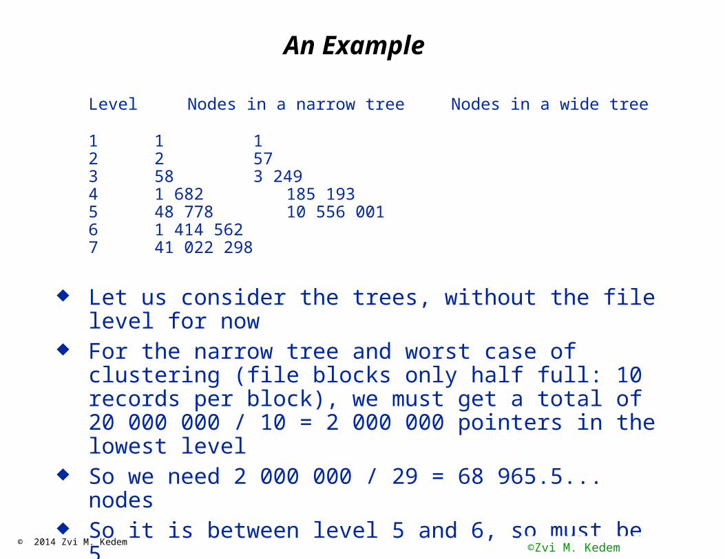
Level Nodes in a narrow tree Nodes in a wide tree
1 1 12 2 573 58 3 2494 1 682 185 1935 48 778 10 556 0016 1 414 5627 41 022 298
Let us consider the trees, without the file level for now For the narrow tree and worst case of clustering (file
blocks only half full: 10 records per block), we must get a total of 20 000 000 / 10 = 2 000 000 pointers in the lowest level
So we need 2 000 000 / 29 = 68 965.5... nodes So it is between level 5 and 6, so must be 5
· Rounding down as before
©Zvi M. Kedem

© 2014 Zvi M. Kedem 71
An Example
Level Nodes in a narrow tree Nodes in a wide tree
1 1 12 2 573 58 3 2494 1 682 185 1935 48 778 10 556 0016 1 414 5627 41 022 298
For the wide tree and best case of clustering (file blocks completely full: 20 records per block), we must get a total of 20 000 000 / 20 = 1 000 000 pointers in the lowest level
so we need 1 000 000 / 57 = 17 543.8… nodes So it is between level 3 and 4, so must be 4
· Rounding up as before
Conclusion: it will be between 5 + 1 = 6 and 4 +1 = 5 levels (including the file level), with this number of block accesses required to access a record.

© 2014 Zvi M. Kedem 72
Finding 10 records
So how many block accesses are needed for reading, say 10 records?
If the 10 records are “random,” then we need possibly close to 60 block accesses to get them, 6 accesses per record.
In practice (which we do not discuss here), somewhat fewer, as it is likely that the top levels of the B-tree are cashed and therefore no need to read them again for each search of one of the 10 records of interest
© 2014 Zvi M. Kedem 73
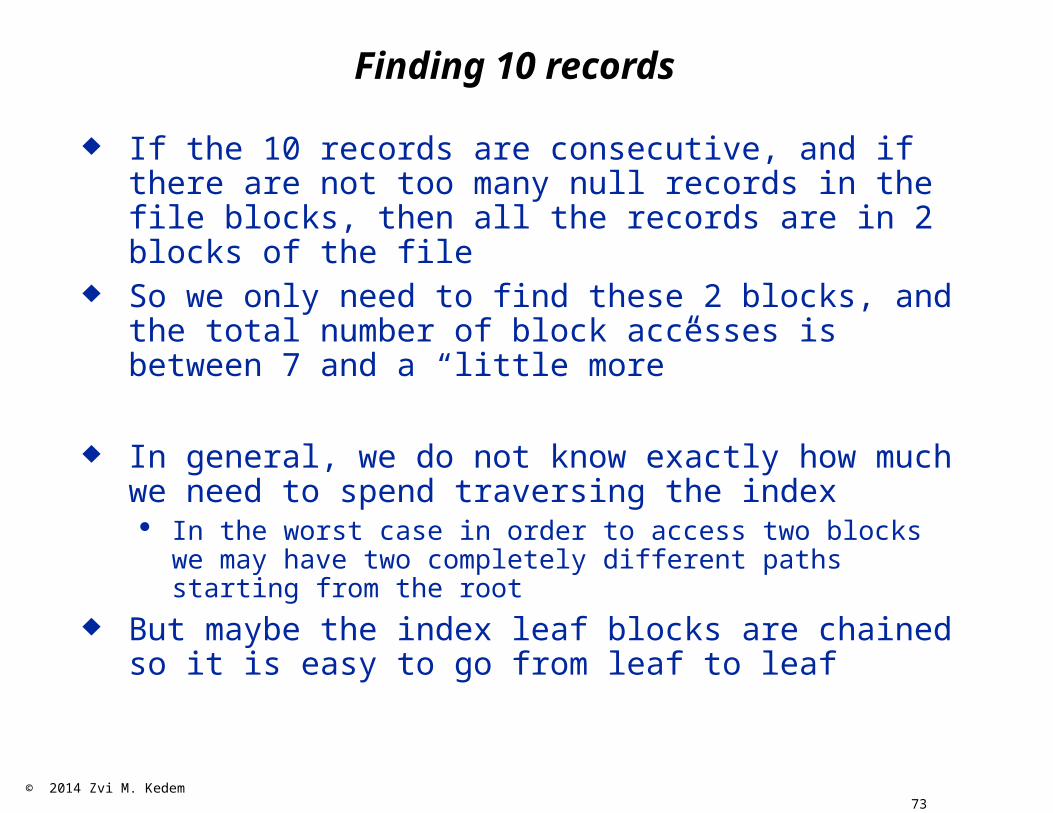
Finding 10 records
If the 10 records are consecutive, and if there are not too many null records in the file blocks, then all the records are in 2 blocks of the file
So we only need to find these 2 blocks, and the total number of block accesses is between 7 and a “little more”
In general, we do not know exactly how much we need to spend traversing the index· In the worst case in order to access two blocks we may have two
completely different paths starting from the root
But maybe the index leaf blocks are chained so it is easy to go from leaf to leaf
© 2014 Zvi M. Kedem 74
An Example
To reiterate:
The first layout resulted in an unclustered file The second layout resulted in a clustered file
Clustering means: “logically closer” records are “physically closer”
More precisely: as if the file has been sorted with blocks not necessarily full and then the blocks were dispersed
So, for a range query the second layout is much better, as it decreases the number of accesses to the file blocks by a factor of between 10 and 20

© 2014 Zvi M. Kedem 75
How About Hashing On A Disk
Same idea
Hashing as in RAM, but now choose B, so that “somewhat fewer” than 20 key values from the file will hash on a single bucket value
Then, from each bucket, “very likely” we have a linked list consisting of only one block
But how do we store the bucket array? Very likely in memory, or in a small number of blocks, which we know exactly where they are
So, we need about 2 block accesses to reach the right record “most of the time”
© 2014 Zvi M. Kedem 76
Index On A Non-Key Field
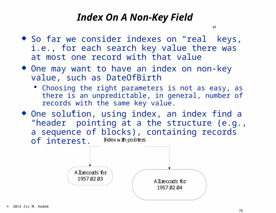
So far we consider indexes on “real” keys, i.e., for each search key value there was at most one record with that value
One may want to have an index on non-key value, such as DateOfBirth· Choosing the right parameters is not as easy, as there is an
unpredictable, in general, number of records with the same key value.
One solution, using index, an index find a “header” pointing at a the structure (e.g., a sequence of blocks), containing records of interest.
All records for1957.02.03 All records for
1957.02.04
Index with pointers

© 2014 Zvi M. Kedem 77
Index On A Non-Key Field: Hashing
The number of (key, pointer) pairs on the average should be “somewhat” fewer than what can fit in a single block
Very efficient access to all the records of interest
47 37 57
47 ……. 47 ……. 47 …….
17
47 ……. 47 …….
key, pointerpairs
blocks with
records

© 2014 Zvi M. Kedem 78
Index On A Non-Key Field: B+-tree
47 ……. 47 ……. 47 …….
47 ……. 47 …….
Bottom Level Of The Tree
pointer supposed to be pointing at the block containing record with key value 47

© 2014 Zvi M. Kedem 79
Primary vs. Secondary Indexes
In the context of clustered files, we discussed a primary index, that is the one according to which a file is physically organized, say SSN
But if we want to efficiently answer queries such as:· Get records of all employees with salary between 35,000 and
42,000· Get records of all employees with the name: “Ali”
For this we need more indexes, if we want to do it efficiently
They will have to be put “on top” of our existing file organization.· The primary file organization was covered above, it gave the
primary index
We seem to need to handle range queries on salaries and non-range queries on names
We will generate secondary indexes

© 2014 Zvi M. Kedem 80
Secondary Index On Salary
The file’s primary organization is on SSN So, it is “very likely” clustered on SSN, and therefore it
cannot be clustered on SALARY Create a new file of variable-size records of the form:
(SALARY)(SSN)*
For each existing value of SALARY, we have a list of all SSN of employees with this SALARY.
This is clustered file on SALARY

© 2014 Zvi M. Kedem 81
Secondary Index On Salary
Create a B+-tree index for this file Variable records, which could span many blocks are
handled similarly to the way we handled non-key indexes This tree together with the new file form a secondary
index on the original file Given a range of salaries, using the secondary index we
find all SSN of the relevant employees Then using the primary index, we find the records of these
employees· But they are unlikely to be contiguous, so may need “many” block
accesses

© 2014 Zvi M. Kedem 82
Secondary Index on Name
The file’s primary organization is on SSN So, it is “very likely” clustered on SSN, and therefore it
cannot be clustered on NAME Create a file of variable-size records of the form:
(NAME)(SSN)*
For each existing value of NAME, we have a list of all SSN of employees with this NAME.
Create a hash table for this file This table together with the new file form a secondary
index on the original file Given a value of name, using the secondary index we find
all SSN of the relevant employees Then using the primary index, we find the records of these
employees

© 2014 Zvi M. Kedem 83
Index On Several Fields
In general, a single index can be created for a set of columns
So if there is a relation R(A,B,C,D), and index can be created for, say (B,C)
This means that given a specific value or range of values for (B,C), appropriate records can be easily found
This is applicable for all type of indexes

© 2014 Zvi M. Kedem 84
Symbolic vs. Physical Pointers
Our secondary indexes were symbolic
Given value of SALARY or NAME, the “pointer” was primary key value
Instead we could have physical pointers
(SALARY)(block address)* and/or (NAME)(block address)*
Here the block addresses point to the blocks containing the relevant records
Access more efficient as we skip the primary index Maintaining more difficult
· If primary index needs to be modified (new records inserted, causing splits, for instance) need to make sure that physical pointers properly updated

© 2014 Zvi M. Kedem 85
How About SQL?
Most commercial database systems implement indexes Assume relation R(A,B,C,D) with primary key A Some typical statements in commercial SQL-based
database systems· CREATE UNIQUE INDEX index1 on R(A); unique implies that this
will be a “real” key, just like UNIQUE is SQL DDL· CREATE INDEX index2 ON R(B ASC,C)· CREATE CLUSTERED INDEX index3 on R(A)· DROP INDEX index4
Generally some variant of B+ tree is used (not hashing)· In fact generally you cannot specify whether to use B+ -trees or
hashing

© 2014 Zvi M. Kedem 86
Oracle SQL
Generally:· When a PRIMARY KEY is declared the system generates a
primary index using a B+-treeUseful for retrieval and making sure that this indeed is a primary key (two different rows cannot have the same key); in fact two identical rows are not permitted by Oracle also
· When UNIQUE is declared, the system generates a secondary index using a B+-treeUseful as above
It is possible to specify hash indexes using, so called, HASH CLUSTERs· Useful for fast retrieval, particularly on equality (or on a very small
number of values)
It is possible to specify bit-map indexes, particularly useful for querying databases (not modifying them—that is, useful in a “warehouse” environment)

© 2014 Zvi M. Kedem 87
Bitmap Index
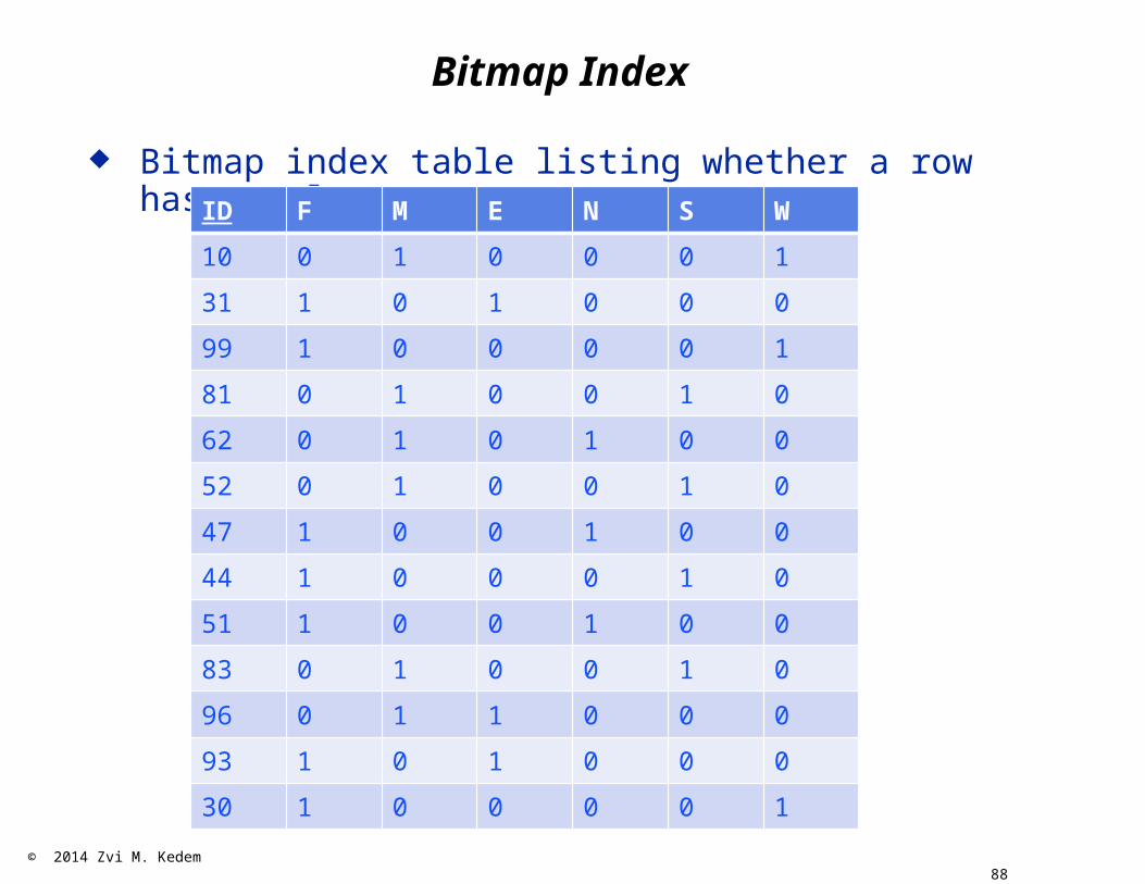
Assume we have a relation (table) as follows:ID Sex Region Salary
10 M W 450
31 F E 321
99 F W 450
81 M S 356
62 M N 412
52 M S 216
47 F N 658
44 F S 987
51 F N 543
83 M S 675
96 M E 412
93 F E 587
30 F W 601
© 2014 Zvi M. Kedem 88
Bitmap Index
Bitmap index table listing whether a row has a valueID F M E N S W
10 0 1 0 0 0 1
31 1 0 1 0 0 0
99 1 0 0 0 0 1
81 0 1 0 0 1 0
62 0 1 0 1 0 0
52 0 1 0 0 1 0
47 1 0 0 1 0 0
44 1 0 0 0 1 0
51 1 0 0 1 0 0
83 0 1 0 0 1 0
96 0 1 1 0 0 0
93 1 0 1 0 0 0
30 1 0 0 0 0 1
© 2014 Zvi M. Kedem 89
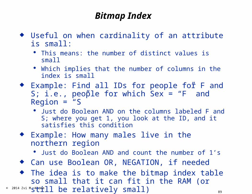
Bitmap Index
Useful on when cardinality of an attribute is small:· This means: the number of distinct values is small· Which implies that the number of columns in the index is small
Example: Find all IDs for people for F and S; i.e., people for which Sex = “F” and Region = “S”· Just do Boolean AND on the columns labeled F and S; where you
get 1, you look at the ID, and it satisfies this condition
Example: How many males live in the northern region· Just do Boolean AND and count the number of 1’s
Can use Boolean OR, NEGATION, if needed The idea is to make the bitmap index table so small that it
can fit in the RAM (or still be relatively small)· So operations are very efficient
But, the ID field could be large Solution: two tables, each smaller than the original one

© 2014 Zvi M. Kedem 90
Optimization: Maintain 2 Smaller StructuresWith Implicit Row Pairing
ID
10000000400567688782345
31000000400567688782345
99000000400567688782345
81000000400567688782345
62000000400567688782345
52000000400567688782345
47000000400567688782345
44000000400567688782345
51000000400567688782345
83000000400567688782345
96000000400567688782345
93000000400567688782345
30000000400567688782345
F M E N S W
0 1 0 0 0 1
1 0 1 0 0 0
1 0 0 0 0 1
0 1 0 0 1 0
0 1 0 1 0 0
0 1 0 0 1 0
1 0 0 1 0 0
1 0 0 0 1 0
1 0 0 1 0 0
0 1 0 0 1 0
0 1 1 0 0 0
1 0 1 0 0 0
1 0 0 0 0 1
© 2014 Zvi M. Kedem 91
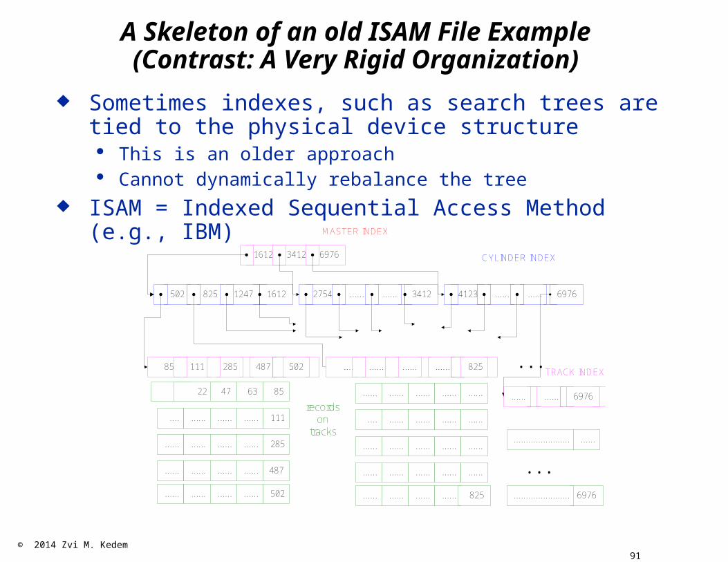
A Skeleton of an old ISAM File Example(Contrast: A Very Rigid Organization)
Sometimes indexes, such as search trees are tied to the physical device structure· This is an older approach· Cannot dynamically rebalance the tree
ISAM = Indexed Sequential Access Method (e.g., IBM)
34121612 6976
825 502 1247 1612 ......2754 ...... 3412 ......4123 ...... 6976
111 85 285 487 502
...... .... ...... ...... 825
MASTER INDEX
CYLINDER INDEX
TRACK INDEX...
4 22 47 63 85
.... ...... ...... ...... 111
...... ...... ...... ...... 285
...... ...... ...... ...... 487
...... ...... ...... ...... 502
...... ...... ...... ...... ......
...... ...... 6976
...... ...... ...... ...... ......
.......................... ......
6976.......................
...... ...... ...... ...... ......
.... ...... ...... ...... ......
...... ...... ...... ...... 825
recordson
tracks

© 2014 Zvi M. Kedem 92
Query Execution Concepts

© 2014 Zvi M. Kedem 93
Execution Plan
Given a reasonably complex query there may be various ways of executing it
Good Database Management Systems (such as newer versions of Oracle)· Maintain statistical information about the database· Use this information to decide how to execute the query
Given a query, they decide on an execution plan

© 2014 Zvi M. Kedem 94
When to Use Indexes To Find Records
When you expect that it is cheaper than simply going through the file
How do you know that? Make profiles, estimates, guesses, etc.
Note the importance of clustering in greatly decreasing the number of block accesses· Example, if there are 1,000 blocks in the file, 100 records per
block (100,000 records in the file), and– There is a hash index on the records– The file is unclustered (of course)
· To find records of interest, we need to read at least all the blocks that contain such records
· To find 50 (very small fraction of) records, perhaps use an index, as these records are in about (maybe somewhat fewer) 50 blocks, very likely
· To find 2,000 (still a small fraction of) records, do not use an index, as these records are in “almost as many as” 1,000 blocks, very likely, so it is faster to traverse the file and read 1000 blocks (very likely) than use the index

© 2014 Zvi M. Kedem 95
A Sharp Example
We have a relation Employee(SSN,BirthDate,Sex) We have a primary index on SSN and secondary indexes
on BirthDate and Sex We have a query
SELECT SSNFROM EmployeeWHERE BirthDate = ‘1982-05-03’ AND Sex = ‘Female’;
Two choices· Bring all the blocks containing ‘1982-05-03’ and then pick out the
records containing ‘Female’· Bring all the blocks containing ‘Female’ (which could be all the
blocks) and then pick out the records containing ‘1982-05-03’
If the systems knows that about 50% of the employees are Female, the second choice is very bad, but the first choice is likely to be very good
But the system must profile the database, or the programmer needs to set/influence the execution plan

© 2014 Zvi M. Kedem 96
Computing Conjunction Conditions
A simple “more general” example: R(A,B) SELECT *
FROM RWHERE A = 1 AND B = 'Mary';
Assume the database has indexes on A and on B This means, we can easily find
· All the blocks that contain at least one record in which A = 1· All the blocks that contain at least one record in which B = ‘Mary’
A reasonably standard solution· DB picks one attribute with an index, say A· Brings all the relevant blocks into memory (those in which there is
a record with A = 1)· Selects and outputs those records for which A = 1 and B = ‘Mary’
© 2014 Zvi M. Kedem 97
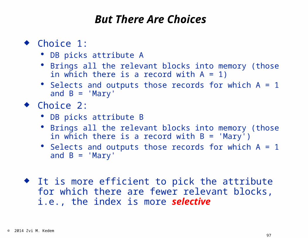
But There Are Choices
Choice 1:· DB picks attribute A· Brings all the relevant blocks into memory (those in which there is
a record with A = 1)· Selects and outputs those records for which A = 1 and B = 'Mary'
Choice 2:· DB picks attribute B· Brings all the relevant blocks into memory (those in which there is
a record with B = 'Mary')· Selects and outputs those records for which A = 1 and B = 'Mary'
It is more efficient to pick the attribute for which there are fewer relevant blocks, i.e., the index is more selective

© 2014 Zvi M. Kedem 98
But There Are Choices
Some databases maintain profiles, statistics helping them to decide which indexes are more selective
But some have a more static decision process· Some pick the first in the sequence, in this case A· Some pick the last in the sequence, in this case B (Oracle used to
do that)
So depending on the system, one of the two below may be much more efficient than the other· SELECT *
FROM RWHERE A = 1 AND B = 'Mary';
· SELECT *FROM RWHERE B = 'Mary' AND A = 1;
So it may be important for the programmer to decide which of the two equivalent SQL statements to specify

© 2014 Zvi M. Kedem 99
Using Both Indexes
DB brings into RAM the identifiers of the relevant blocks (their serial numbers
Intersects the set of identifiers of blocks relevant for A with the set of identifiers of blocks relevant for B
Reads into RAM the identifiers in the intersections and selects and outputs records satisfying the conjunction

© 2014 Zvi M. Kedem 100
Computing A Join Of Two Tables
We will deal with rough asymptotic estimates to get the flavor· So we will make simplifying assumptions, which still provide the
intuition, but for a very simple case
We have available RAM of 3 blocks We have two tables R(A,B), S(C,D) Assume no indexes exist There are 1,000 blocks in R There are 10,000 blocks in S We need (or rather DB needs) to compute
SELECT * FROM R, SWHERE R.B = S.C;

© 2014 Zvi M. Kedem 101
A Simple Approach
Read 2 blocks of R into memory· Read 1 block of S into memory· Check for join condition for all the “resident” records of R and S· Repeat a total of 10,000 times, for all the blocks of S
Repeat for all subsets of 2 size of R, need to do it total of 500 times
Total reads: 1 read of R + 500 reads of S = 5,001,000 block reads
Essentially quadratic in the size of the files

© 2014 Zvi M. Kedem 102
A Simple Approach
Read 2 blocks of S into memory· Read 1 block of R into memory· Check for join condition for all the “resident” records of R and S· Repeat a total of 1,000 times, for all the blocks of R
Repeat for all subsets of 2 size of S, need to do it total of 5,000 times
Total reads: 1 read of S + 5,000 reads of R = 5,010,000 block reads
Essentially quadratic in the size of the files
© 2014 Zvi M. Kedem 103
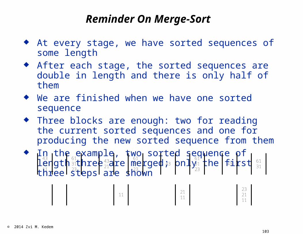
Reminder On Merge-Sort
At every stage, we have sorted sequences of some length After each stage, the sorted sequences are double in
length and there is only half of them We are finished when we have one sorted sequence Three blocks are enough: two for reading the current
sorted sequences and one for producing the new sorted sequence from them
In the example, two sorted sequence of length three are merged; only the first three steps are shown
432111
613123
4321
613123
11
43613123
2111
436131
232111

© 2014 Zvi M. Kedem 104
Merge-Join
If R is sorted on B and S is sorted on C, we can use the merge-sort approach to join them
While merging, we compare the current candidates and output the smaller (or any, if they are equal)
While joining, we compare the current candidates, and if they are equal, we join them, otherwise we discard the smaller
In the example below (where only the join attributes are shown, we would discard 11 and 43 and join 21 with 21 and 61 with 61
612111
614321
© 2014 Zvi M. Kedem 105
Merge-Join
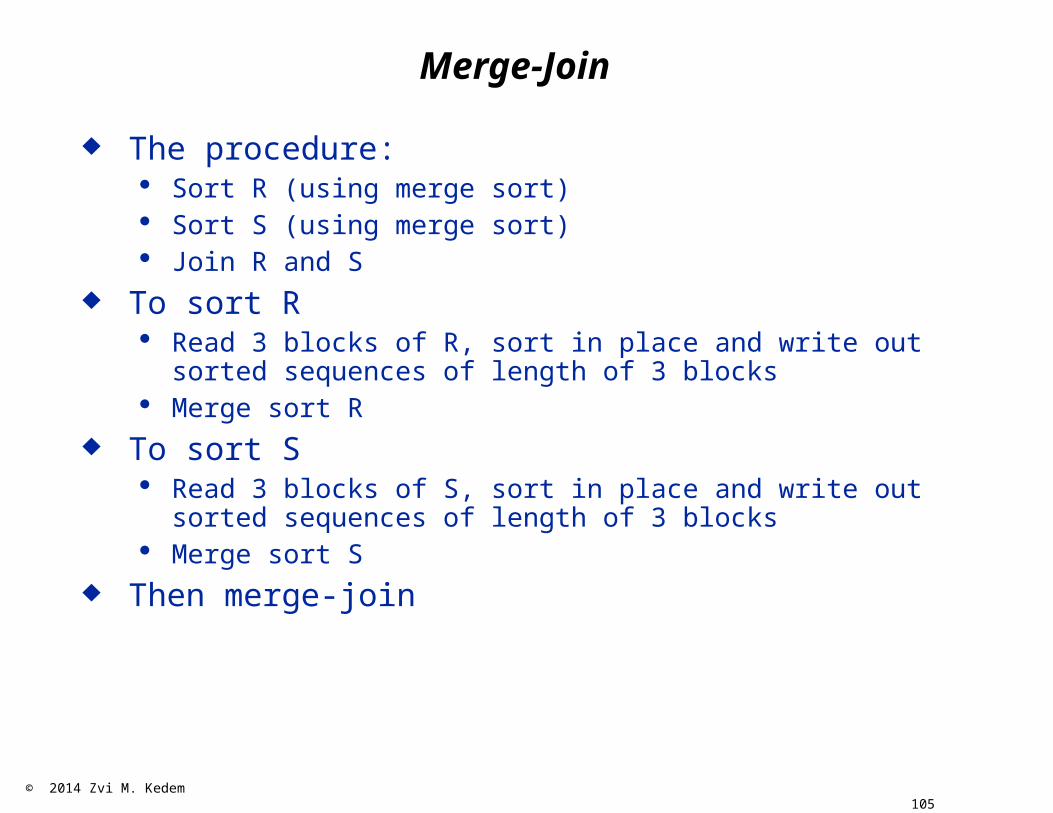
The procedure:· Sort R (using merge sort)· Sort S (using merge sort)· Join R and S
To sort R· Read 3 blocks of R, sort in place and write out sorted sequences
of length of 3 blocks· Merge sort R
To sort S· Read 3 blocks of S, sort in place and write out sorted sequences
of length of 3 blocks· Merge sort S
Then merge-join

© 2014 Zvi M. Kedem 106
Performance Of Merge-Join
To sort R, ceiling of log2 1000 = 10 passes, where pass means read and write
To sort S, ceiling of log2 10000 = 14 passes, where pass means read and write
Once we have sorted R and S, to merge-join R and S, one pass on each of R and S (as we join on keys, so each row of R either has one row of S matching, or no matching row at all)· Specifically we read the first block of R and the first block of S and
join what we can and then read the next block of either R or S or both depending on which is completely processed
· When a block of the join is full, write it out and start a new block
Cost· 10 passes to sort R: 20000 block accesses (reads and writes)· 14 passes to sort S: 280000 block accesses (reads and writes)· joining: 1000 for reading R, 10000 for reading S, at most 1000 for
writing the join

© 2014 Zvi M. Kedem 107
Hash-Join
Sorting could be considered in this context similar to the creation of an index
Hashing can be used too, though more tricky to do in practice and therefore less popular

© 2014 Zvi M. Kedem 108
Order Of Joins Matters
Consider a database consisting of 3 relations· Lives(Person, City) about people in the US, about 300,000,000
tuples· Oscar(Person) about people in the US who have won the Oscar,
about 1,000 tuples· Nobel(Person) about people in the US who have won the Nobel,
about 100 tuples
How would you answer the question, trying to do it most efficiently “by hand”?
Produce the relation Good_Match(Person1,Person2) where the two Persons live in the same city and the first won the Oscar prize and the second won the Nobel prize
How would you do it using SQL?
© 2014 Zvi M. Kedem 109
Order Of Joins Matters
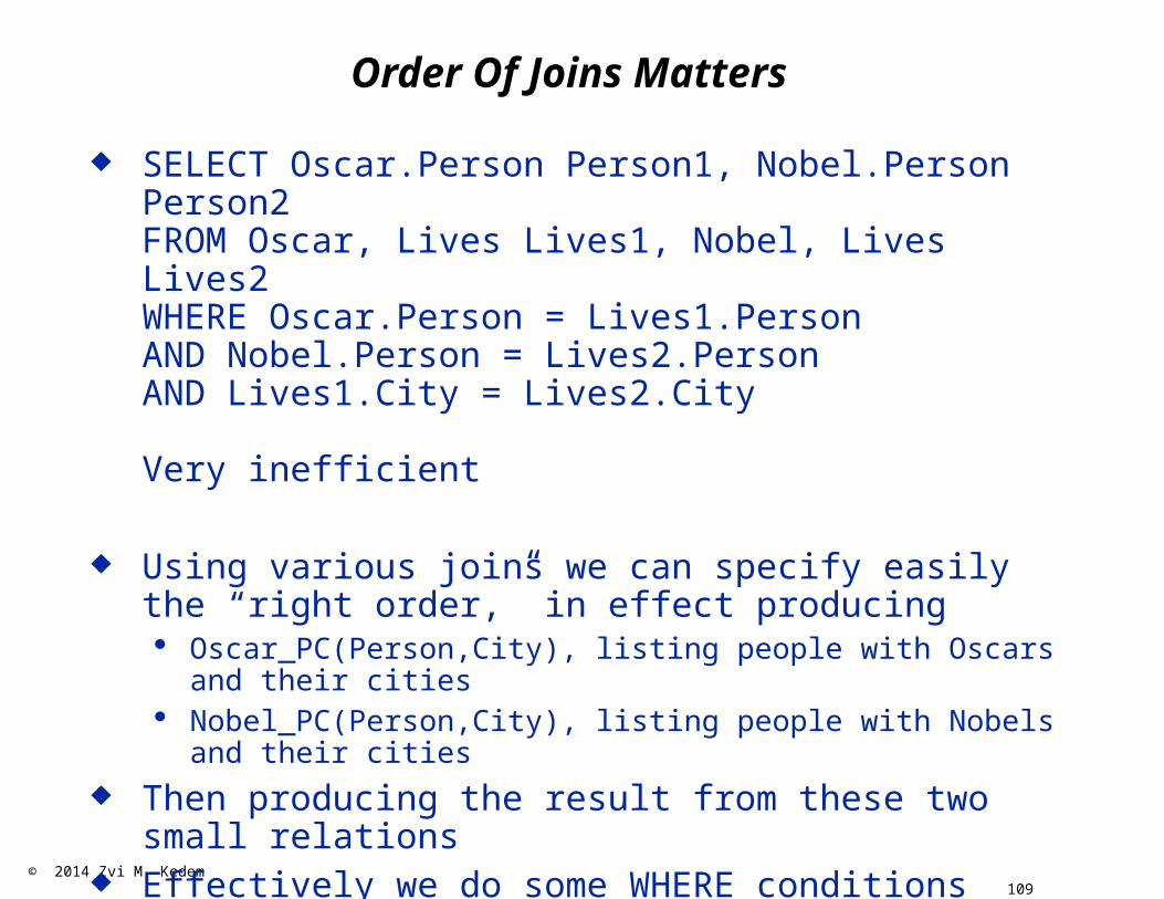
SELECT Oscar.Person Person1, Nobel.Person Person2FROM Oscar, Lives Lives1, Nobel, Lives Lives2WHERE Oscar.Person = Lives1.Person AND Nobel.Person = Lives2.PersonAND Lives1.City = Lives2.City
Very inefficient
Using various joins we can specify easily the “right order,” in effect producing · Oscar_PC(Person,City), listing people with Oscars and their cities· Nobel_PC(Person,City), listing people with Nobels and their cities
Then producing the result from these two small relations Effectively we do some WHERE conditions earlier, rather
than later This is much more efficient

© 2014 Zvi M. Kedem 110
Granularity Of Locks(Simplified Granularity-Based Locking)
See https://docs.oracle.com/cd/E17952_01/refman-5.1-en/innodb-lock-modes.html
There are 4 types of locks and their compatibility matrix is
IS stands for “Intent Shared” IX stands for “Intent eXclusive”
As usual, the matrix states what two transactions can hold simultaneously, a transaction can hold any set of locks on an item (as long as not conflicting with other transactions)
Type N S X IS IX
N Yes Yes Yes Yes Yes
S Yes Yes No Yes No
X Yes No No No No
IS Yes Yes No Yes Yes
IX Yes No No Yes Yes

© 2014 Zvi M. Kedem 111
Granularity Of Locks(Simplified Granularity-Based Locking)
Assume one table R and five rows 1, 2, 3, 4, 5. The items that can be locked are R, 1, 2, 3, 4, 5. To have write access to all of R, a transaction needs an X-
lock on R To have a read access on all of R, a transaction needs an
X-lock or an S-lock on R To have write access to a row of R, a transaction needs
an X-lock on that row To have a read access on a row of R, a transaction needs
an X-lock or an S-lock on that row To set an X-lock on a row of R, a transaction needs an IX-
lock on R To set an S-lock on a row of R, a transaction needs an IX-
lock or an IS-lock on R Locking is top to bottom; unlocking is bottom to top

© 2014 Zvi M. Kedem 112
Granularity Of Locks(Simplified Granularity-Based Locking)
The goal is to prevent situations such as· T1 holds X-lock on R and T2 holds an S-lock on 1· T1 holds X-lock on R and T2 holds an X-lock on 1· T1 holds S-lock on R and T2 holds an X-lock on 1
The goal is to permit situations such as· T1 holds S-lock on R and T2 holds an S-lock on 1· T1 holds S-lock on 1 and T2 holds an X-lock on 2· T1 holds X-lock on 1 and T2 holds an X-lock on 2
© 2014 Zvi M. Kedem 113
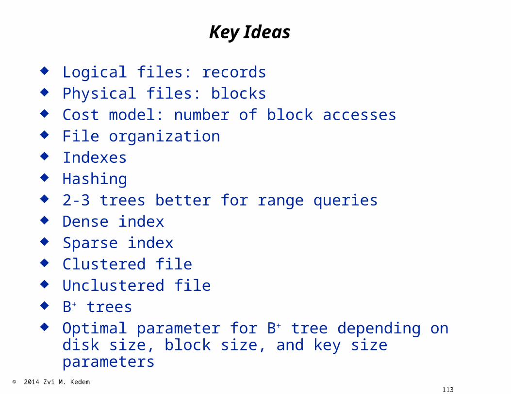
Key Ideas
Logical files: records Physical files: blocks Cost model: number of block accesses File organization Indexes Hashing 2-3 trees better for range queries Dense index Sparse index Clustered file Unclustered file B+ trees Optimal parameter for B+ tree depending on disk size,
block size, and key size parameters

© 2014 Zvi M. Kedem 114
Key Ideas
Best: clustered file and sparse index Hashing on disk Index on non-key fields Secondary index Use index for searches if it is likely to help SQL support Bitmap index Need to know how the system processes queries How to use indexes for some queries How to process some queries Merge Join Hash Join Order of joins Cutting down relations before joining them