A COMPARATIVE SIMULATION STUDY OF A MODIFIED HOMEPLUG AV PLC SYSTEM WITH NOVEL ADAPTIVE BIT LOADING AND LDPC CODES

By

GAUTHAM PRASAD

A THESIS PRESENTED TO THE GRADUATE SCHOOL

OF THE UNIVERSITY OF FLORIDA IN PARTIAL FULFILLMENT OF THE REQUIREMENTS FOR THE DEGREE OF

MASTER OF SCIENCE

UNIVERSITY OF FLORIDA

2014

© 2014 Gautham Prasad

To my parents and The Lord Almighty

4

ACKNOWLEDGMENTS

I would like to express deep gratitude to my advisor, Prof. Haniph Latchman. It is

his constant guidance and encouragement that has brought me this far in my research.

I am thankful to Dr. Richard Newman and Dr. Janise McNair for accepting to

serve as members of my thesis committee.

I thank my colleagues at the Laboratory for Information Systems and

Telecommunication (LIST) for all the insightful discussions we have had on this

wonderful and ever growing field of Power Line Communications (PLC).

I am fortunate to have found lovely friends at Gainesville who have shared my

happiness and sorrows and encouraged me at all times.

I owe many thanks to University of Florida Information Technology (UFIT) for

providing access to MATLAB.

I am extremely grateful to my parents for the unconditional love and support they

have given me. I would not be where I am without their encouragement.

5

TABLE OF CONTENTS page

ACKNOWLEDGMENTS .................................................................................................. 4

LIST OF TABLES ............................................................................................................ 7

LIST OF FIGURES .......................................................................................................... 8

LIST OF ABBREVIATIONS ............................................................................................. 9

ABSTRACT ................................................................................................................... 11

CHAPTER

1 INTRODUCTION .................................................................................................... 13

2 LITERATURE REVIEW .......................................................................................... 18

HomePlug Powerline Alliance and HomePlug Standards ....................................... 18 Low Density Parity Check Codes ............................................................................ 19

Encoding .......................................................................................................... 20

Decoding .......................................................................................................... 20 Turbo Codes ........................................................................................................... 22

Encoding .......................................................................................................... 22 Decoding .......................................................................................................... 22

HomePlug System with LDPC Encoding ................................................................ 23

3 HOMEPLUG AV SYSTEM MODEL ........................................................................ 26

Scrambler ............................................................................................................... 28

Turbo Convolutional Encoder ................................................................................. 29 ROBO Modes ......................................................................................................... 29

Mapping .................................................................................................................. 30 Multicarrier Modulation Using OFDM ...................................................................... 31 Tone Mask .............................................................................................................. 32

4 MODIFIED ADAPTIVE BIT LOADING ALGORITHM .............................................. 33

Review of Existing Bit Loading Algorithms .............................................................. 33 Water Filling Algorithm ..................................................................................... 34 WLK Algorithm ................................................................................................. 35

Drawbacks for PLC Implementation ................................................................. 36 Modified Adaptive Modulation Algorithm ................................................................. 37 Simulation Results and Performance Evaluation .................................................... 37

5 LDPC AND TURBO CODES WITH REAL POWERLINE NOISE ........................... 43

6

LDPC System Implementation ................................................................................ 43

Turbo Encoding and Decoding ............................................................................... 43 Performance Evaluation of LDPC and Turbo Codes With Real Powerline Noise ... 44

6 LDPC AND TURBO CODES ON A REAL POWERLINE CHANNEL AND HOMEPLUG AV STANDARDS .............................................................................. 48

Encoding and Decoding Process for LDPC ............................................................ 49 Simulation Environment and System Implementation ............................................. 50

System Parameters Specified by HPAV ........................................................... 50

Implementation of Forward Error Correction Coding ........................................ 52 Digital Modulation ............................................................................................. 52 Carrier Notching for FCC Compliance .............................................................. 53 OFDM ............................................................................................................... 53

Guard Intervals (GI) .......................................................................................... 53 Signal Power .................................................................................................... 53

Receiver ........................................................................................................... 54 PLC Channel and Noise Effects ....................................................................... 54

Simulation Results and Performance Evaluation .................................................... 58

7 QUASI CYCLIC – LOW DENSITY PARITY CHECK CODES (QC-LDPC) ............. 61

8 CONCLUSIONS AND FUTURE WORK ................................................................. 63

LIST OF REFERENCES ............................................................................................... 66

BIOGRAPHICAL SKETCH ............................................................................................ 68

7

LIST OF TABLES

Table page 4-1 Data rates for different algorithms and error rates .............................................. 42

6-1 Error rates for different FEC schemes ................................................................ 59

8

LIST OF FIGURES

Figure page 2-1 Tanner graph for an LDPC code ......................................................................... 21

3-1 Block diagram of the HPAV PHY Layer .............................................................. 28

4-1 Bit loading profile using water filling algorithm .................................................... 39

4-2 Bit loading profile using WLK algorithm .............................................................. 40

4-3 Bit loading profile using modified WLK algorithm ................................................ 41

5-1 Noise samples seen on powerline channels ....................................................... 45

5-2 Error rate performance of LDPC and Turbo codes under powerline noise environment ........................................................................................................ 46

6-1 PLC network configuration for channel measurement ........................................ 55

6-2 Impulse responses of the PLC channels ............................................................ 56

6-3 Frequency responses of the PLC channels ........................................................ 57

6-4 Power Spectral Density of the transmitted and the received signal .................... 58

6-5 BER performance of LDPC and Turbo codes on a real powerline channel ........ 59

9

LIST OF ABBREVIATIONS

ABL

APP

ARQ

AWGN

BEC

BER

BPSK

COMSOC

DFT

FCC

FDM

FEC

FFT

HD-PLC

HPAV

HPGP

ICI

IDFT

IFFT

ISI

ITU

LDPC

LUT

Adaptive Bit Loading

A Posteriori Probability

Automatic Repeat Request

Additive White Gaussian Noise

Backward Error Correction

Bit Error Rate

Binary Phase Shift Keying

Communications Society

Discrete Fourier Transform

Federal Communications Commission

Frequency Division Multiplexing

Forward Error Correction

Fast Fourier Transform

High Definition – Power Line Communication

HomePlug AV

HomePlug Green PHY

Inter Carrier Interference

Inverse Discrete Fourier Transform

Inverse Fast Fourier Transform

Inter Symbol Interference

International Telecommunication Union

Low Density Parity Check

Look Up Table

10

MAC

MIMO

MPDU

NEK

OFDM

PCCC

PLC

PSD

QAM

QC-LDPC

QPSK

SCCC

SNR

TCC

Medium Access Control

Multiple Input Multiple Output

MAC Protocol Data Unit

Network Encryption Key

Orthogonal Frequency Division Multiplexing

Parallel Concatenated Convolutional Codes

Powerline Communication

Power Spectral Density

Quadrature Amplitude Modulation

Quasi Cyclic Low Density Parity Check

Quadrature Phase Shift Keying

Serial Concatenated Convolutional Codes

Signal to Noise Ratio

Turbo Convolutional Codes

11

Abstract of Thesis Presented to the Graduate School of the University of Florida in Partial Fulfillment of the Requirements for the Degree of Master of Science

A COMPARATIVE SIMULATION STUDY OF A MODIFIED HOMEPLUG AV PLC

SYSTEM WITH NOVEL ADAPTIVE BIT LOADING AND LDPC CODES

By

Gautham Prasad

May 2014

Chair: Haniph A. Latchman Major: Electrical and Computer Engineering

Data communication through existing power lines has been the subject of much

research over the past decade. Different industry collaborations have tried to develop

standards for Power Line Communication (PLC) and the HomePlug AV (HPAV)

standard has been the most successful so far. HPAV uses Orthogonal Frequency

Division Multiplexing (OFDM) to achieve multicarrier modulation and adaptive bit

loading on each of these orthogonal sub carriers. Data rates can be improved by using

novel adaptive bit loading strategies to exploit the frequency selective nature of the

harsh powerline channel. Various bit loading algorithms are simulated and a new

algorithm is proposed to boost the data rates. Analysis and simulation results reveal a

43% improvement in the data rates from 34.44 Mbps to 49.39 Mbps for a real powerline

channel with an un-encoded BER of 10-2.

HPAV systems also use turbo codes for Forward Error Correction (FEC) as

opposed to Low Density Parity Check Codes (LDPC) because of its high performance

at low Signal to Noise Ratios (SNR) which is common in longer powerline runs. The

successful implementation of turbo codes in HPAV also resulted in IEEE 1901

standards incorporating turbo codes for FEC. However, turbo codes are licensed and

12

usually require a patent fee to be paid for each turbo code enabled product. The

objective of this project is to examine whether the unlicensed LDPC codes could be a

viable FEC alternative for HPAV systems.

Extensive analysis and simulation results are provided to show that the LDPC

codes of block length 32400, improve the Bit Error Rates (BER) by 28% even at a low

SNR of 1 dB. However, increase in block length is accompanied by higher memory

requirement. A simple implementation of low-memory LDPC codes in the form of Quasi-

Cyclic LDPC (QC-LDPC) is also discussed. All simulations are run on 10 different real

powerline channels with HPAV specifications.

13

CHAPTER 1 INTRODUCTION

The ability to communicate using the existing power lines, has made Power Line

Communication (PLC) an attractive topic for researchers and engineers from industry,

universities and utility companies [1]. PLC is used in different fields from smart grids and

automatic meter reading to in-home multimedia communication. Utility organizations

have historically given immense attention towards PLC. Power lines were initially used

for load management. Lately, however, utility companies have started employing power

line communication to read electric meters from a distance. Power lines can also be

adopted and adapted to broadcast information to all users, selectively turn on and off

certain networks, and gather statistics and other such applications. Many utility

companies are investing their research attention on such areas which fall under the

category of “Smart Grid”. Home automation and intelligent homes are also a budding

area in the field of PLC. Power lines serve as an ideal medium to turn on/off a burglar

alarm system and home appliances. “Smart appliances” are also gaining industry

attention because of the ease it provides for a day-to-day life. For example, a

refrigerator monitors the contents level of a beverage and once it nears emptiness, it

transmits signal on the power line to order fresh supply.

On the other hand power lines are also used for in-home entertainment; mainly

multimedia communication. Local area multi-user gaming, High Definition (HD) video

streaming are applications which demand high speed point-to-point communication

inside a house/building. Data rates obtained by wireless routers are inadequate and

laying new cables such as Cat5E or other Ethernet cables throughout the house

becomes tedious. PLC serves as a viable alternative in such cases providing high

14

speed broadband data communication over existing infrastructure. For applications

such as smart grids, power constraints and reliability play a major role as opposed to

data rates; whereas for multimedia applications, high speeds are critical.

Different industry collaborations have tried to propose different standards for

PLC. High Definition – Power Line Communication (HD-PLC), HomePlug Powerline

Alliance (HPA), G.hn are some of the more popular ones. The International

Telecommunication Union (ITU) adopted the G.hn/G.9960 as a standard powerline

communication. HD-PLC uses Wavelet based OFDM for multi carrier modulation as

opposed to the conventional OFDM used by the HomePlug standards. The FEC

encoding schemes applied by these two competing standards are also different. While

the HD-PLC uses LDPC codes for error correction, HomePlug systems employ Turbo

codes for FEC. However, the standards developed by HPA have been the most

successful so far. There are more than 100 million HomePlug modems deployed to date

and these numbers are continuously increasing [2]. The efficient implementation of

Turbo codes in HPAV systems prompted IEEE 1901 standards to incorporate them as

FEC.

HomePlug Green PHY (HPGP) addresses the low power needs of smart grids

and yet provides speeds up to 10 Mbps [3]. On the other hand, HomePlug 1.0, HPAV

and HPAV2 have provided data rates up to 1.5 Gbps catering to the needs of high

speed applications such as in-home multimedia communication. HomePlug 1.0,

released in 2001 by HPA, achieved speeds of 14 Mbps. This used a small frequency

range of 4.5 MHz – 21 MHz and a concatenation of Viterbi and Reed-Solomon codes

for FEC [4]. Data rates were significantly improved to about 200 Mbps in the

15

subsequent release, HPAV, in 2005 [5]. Similar frequency band was used (1.8 MHz –

30 MHz) but improvements were made to support modulation schemes up to 1024 –

QAM. This helped in improving the data rates drastically. More recently, HPAV2 has

been released, which uses a higher bandwidth from 2- 80 MHz and provides speeds up

to 1.5 Gbps.

IEEE Communications Society (COMSOC) sponsored the P1901 project to

define a globally compatible standard for high speed powerline communication [2]. The

working committee selected a consolidated proposal from HPA and HD-PLC Alliance

and provided the IEEE 1901 standard which represents a compromise between the

conventional OFDM based HPAV and Wavelet OFDM based HD-PLC PHY used in HD-

PLC products. IEEE 1901 specifies both PHYs as optional with an Inter System

Protocol (ISP) which provides coexistence but not interoperability between the two

realizations.

There are various factors that affect the data rates provided by these systems.

Modulation schemes used, error correction strategies employed and MAC protocols

implemented, determine the eventual throughput of the system. The modulation scheme

used, determines the number of bits that are transmitted in a given period of time.

Higher the modulation scheme, higher is the bit rate. However, with increase in

modulation scheme, the error rates also increase. Hence, the modulation schemes

need to be chosen intelligently and adaptively such that the error rates are near static.

Different adaptive bit loading algorithms that have been proposed are evaluated in

Chapter 4. A new bit loading algorithm is also proposed based on the best performing

state-of-the-art bit loading algorithm to suit HPAV systems.

16

One of the major factors assisting in the improvement of throughput and

enhancing the reliability of data transmission is the FEC. Error correction codes can

mainly be divided into two parts:

1. Block codes 2. Convolutional codes

Block codes generate code words by consuming message bits in blocks. The

encoder encodes the message bits with redundant parity check bits, generally

appended to the message, and produces the code words in blocks. Change in block

lengths usually results in change in the code word lengths for static error

correction/detection performance. The size of the input block and the code word block is

characterized by code rate. Code rate is the ratio of the redundant bits added by the

encoder to the code word length. The number of redundant bits added can be

calculated by the difference of the codeword length and the length of the message.

LDPC codes fall under this category of block codes. A discussion and analysis of the

effects of block lengths and code rates on error correction performance is presented in

Chapter 5.

Since the block codes receive the message and generate code words in blocks,

a buffer is generally required to store data at the input. However, there are applications

which demand serial I/O of data and a buffer becomes undesirable [6]. The use of

convolutional codes is most suitable in such cases. A convolutional encoder pursues

the input bits serially as it enters the encoder. Most of the convolutional encoders are

characterized by a generator polynomial. This polynomial can be represented in terms

of shift registers or delay elements. Turbo Convolutional Codes (TCC), used in the

HPAV and IEEE 1901 standards, fall under this category.

17

HomePlug 1.0 used a concatenation of Viterbi and Reed-Solomon codes for

FEC. However, with increase in the number of OFDM sub channels and use of higher

modulation schemes in HPAV, there was a need to improve FEC. The state-of-the-art

FEC technologies were LDPC and Turbo codes. Turbo codes were chosen for HPAV

systems since they provide better error rate performance at low SNRs, which are

common in longer power line runs required for ‘whole house’ coverage. The latest

release, HPAV2, continues to adopt Turbo codes for FEC. However, the drawback of

using TCC is the patent fees that are usually required to be paid for every turbo code

enabled device manufactured. The purpose of this project is to investigate whether

LDPC codes are a viable alternative to Turbo codes for HPAV systems.

A review of basic encoding and decoding concepts and previous attempts at

evaluating the performance of a HPAV system with LDPC codes, are discussed in

Chapter 2. The complete system model of HPAV is provided in Chapter 3. Chapter 4

focuses on the proposed modified adaptive bit loading strategy developed, and its

comparative performance with the existing bit loading algorithms. Chapter 5 deals with

the error rate comparison between LDPC and Turbo codes under powerline noise

environment. The system performance with LDPC and Turbo codes for a HPAV system

with real powerline channels and their associated noise is discussed in Chapter 6. A

novel implementation of LDPC codes in the form of QC-LDPC is shown in Chapter 7.

Conclusions are given in Chapter 8 and the following chapter presents future work that

could be carried out.

18

CHAPTER 2 LITERATURE REVIEW

HomePlug Powerline Alliance and HomePlug Standards

HPA is the largest and the most established industry group in PLC with about 65

member companies in it. It was established in 2000 to develop and promote powerline

communication solutions. HPA was initially formed to address high speed in-home PLC

and networking applications. As of 2012, there are at least 6 vendors and close to 280

different HomePlug products in the markets with over 100 million products shipped

worldwide [2]. HPA uses a well streamlined process for the development of all its

specifications much on the lines of major standards organizations like the IEEE.

HPA first released the HomePlug 1.0 standards in June 2001 providing data

rates of 14 Mbps and coded PHY Rates of 10 Mbps [4]. Subsequent release of HPAV

improved the data rates drastically to reach up to 200 Mbps with coded PHY of 150

Mbps. All the HomePlug products adhere to the FCC regulations by notching out

carriers in the amateur radio band. The convergence of voice, data and video into a

single device drives the constant need for higher speeds. HPAV2 is the latest release of

HPA and it provides data rates of 1.5 Gbps [9] which is ideal for several high speed

applications such as multimedia communication, HD video streaming etc. HPAV2 uses

an additional extended bandwidth of 30 – 80 MHz along with the 2 – 30 MHz which

HPAV uses. It also grants the use of higher modulation schemes of 4096 – QAM and

encoding schemes of larger code rates, which result in higher data rates. AV2 also uses

Multiple Input Multiple Output (MIMO) beam forming, sending data bits on multiple

streams, and thereby increasing the data rates as well as the reliability of the message.

19

While HPAV2 caters the need of high speed PLC providing data rates of 1.5

Gbps, HPGP addresses the needs of Smart Grid applications. HPGP is developed as a

low-power and low-data rate version of HPAV. HPGP only supports the QPSK

modulation scheme and uses a low rate ½ Turbo code for FEC. The bandwidth and

number of subcarriers used remain the same but since QPSK is the only supported

modulation scheme, only the ROBO modes are permitted. This curtails the data rates

but the accomplished data rate of 10 Mbps is still 40 times faster than the Smart Grid

requirements and 1000 times faster than competing PLC technologies such as PRIME,

or G3 which operate at lower frequencies of less than 500 kHz [3].

HPAV systems use 128-bit encryption for security in place of DES used by HP

1.0, thereby providing high level of security with the sate-of-the-art encryption

mechanism. A Network Encryption Key (NEK) is used to encrypt individual segments as

the MAC Protocol Data Unit (MPDU) is created.

All the products of HomePlug technology after HPAV use Turbo codes for FEC

as opposed to the competing LDPC codes though both nearly approach Shannon limit

[10]. Turbo codes provide better error rate performance when compared to LDPC at low

SNRs which are common in longer PLC propagation runs. The technical merits and de-

merits of both the codes are discussed in the following two sections of this chapter.

Low Density Parity Check Codes

LDPC codes were first introduced by Robert Galleger in 1963 [11]. They are high

performance codes which nearly approach the “Shannon limit” [10]. The core of the

functioning of LDPC codes is the parity check matrix. This is obtained based on the

code words formed using the message bits such that every row represents the equation

used to form the code word and the columns of the matrix indicate the digits in the code

20

word. Only if the k-th digit is present in the i-th equation, will there be a ‘1’ in the (k, i)

position of the parity check matrix. The remaining elements are all set to ‘0’. Hence the

parity check matrix is ‘sparse’ and is called a sparse matrix. Also, the density of ‘1’s in

the matrix is less, which is where LDPC gets its name from.

LDPC codes can be classified as:

Regular LDPC code

Irregular LDPC code

A regular LDPC code satisfies two properties: every digit in the code word is

contained in the same number of generator equations and every generator equation

contains the same number of code symbols [11]. An irregular LDPC code does not have

to satisfy these properties.

Encoding

If u is the message sequence and v is the code word produced by using the

generator matrix G, we get

v = u.G (2-1)

The parity check matrix H is such that it satisfies the following relation

v.HT = 0 (2-2)

The codeword v is of length n and the message word is of length k. Hence the number

of redundant bits added by the encoder is n-k. Such a code is said to be (n, k) code with

a code rate of k/n and a code block length of n.

Decoding

LDPC codes can be graphically represented using Tanner graphs [12]. Decoding

process is completely and effectively defined by Tanner graphs. Tanner graphs are

bipartite graphs with two different types of nodes, one called the variable nodes (v-

21

nodes) and the other is the check nodes (c-nodes). Every row in H is associated to one

particular c-node and a column is associated to one v-node. A c-node k is connected to

a neighboring v-node i if and only if hij in H is set to ‘1’. Therefore, there are n v-nodes

and n-k c-nodes in a Tanner graph. The c-node and v-node information is iteratively

updated and a decision is finally made. A Tanner graph of LDPC codes is shown in

Figure 2-1.

Figure 2-1: Tanner graph for an LDPC code

The sample Tanner graph shown represents the parity check matrix,

H = [

0 11 1

0 11 0

0 01 0

1 00 1

1 0 0 1

0 10 0

0 1 1 0

1 11 0

]

As mentioned in the previous sections, we can observe that every row of H represents

the equation to get a code word and every column represents the equations in which

one particular message bit is involved in. For the example mentioned above, the

22

equations satisfied by the code words, based on which the parity check matrix is

characterized, are:

c2 + c4 + c5 + c8 = 0 (2-3)

c1 + c2 + c3 + c6 = 0 (2-4)

c3 + c6 + c7 + c8 = 0 (2-5)

c 1+ c4 + c5 + c7 = 0 (2-6)

These are c-nodes and the v-nodes that are used in the process of decoding.

Turbo Codes

Turbo codes are high performance codes which nearly approach the Shannon

limit. They were first introduced in 1993 by French Telecom and find current

applications in 3G mobile communications and satellite communication.

Encoding

Turbo encoding is carried out using simple shift registers or delay elements and

adders (usually binary adders, or XOR elements). The shift registers are initially set to

different binary values based on the encoding scheme and the parity check elements

required. The number of shift registers present also decides the number of parity bits

that are appended to the message bits to form the code word and hence dictates the

code rate of the encoding scheme. Every message bit passes through various shift

registers, based on the structure of the encoder, and the code word is generated.

Decoding

The decoder is built on the same lines as the encoder. Depending on the number

of parity bits that are added at the encoder, the number of shift registers and streams

through which the received bit has to pass, also changes.

23

The performance of turbo codes is high because of the randomness that the

encoder brings in and the efficiency with which the decoder can read it back. This is

extremely effective for very noisy channels such as the one we have under

consideration, the powerline channel. Thus we can now already see why the turbo

codes perform at least theoretically better than the LDPC codes at noisy conditions or at

lower SNRs.

HomePlug System with LDPC Encoding

The HomePlug 1.0 systems, released in 2001, used a concatenation of Viterbi

and Reed-Solomon codes for FEC. This was about the time when high performance

codes such as Turbo and LDPC codes were being practically implemented successfully.

The performance of a HomePlug 1.0 system with LDPC encoding was tried out in [13].

However, the system evaluation was done only for the ROBO transmission mode of

HP1.0. Also, the simulations were run on a channel modeled by multipath fading and

impulse noise and not a real power line channel environment. The results showed a

minor improvement in error rates over the FEC already in use by HP1.0 systems. Also,

the implementation of codes with certain algorithms was “difficult” “due to the random

interconnect patterns between the variable and check nodes” [13]. Because of this

hurdle, shortened codes were used for simulations thereby reducing the performance of

the proposed system.

There are other research comparisons made in this topic but under different

simulation environments. The paper [14] concludes that Turbo codes outperforms a

(7200, 4797) regular LDPC code but the simulations are carried out only under AWGN

channel conditions. However, powerline channels are much severe with cyclo stationary

impulse noise affecting the data transmission. In [15], LDPC codes are shown to

24

perform better than their turbo counterparts based on ITU-T specifications but not the

HomePlug scenario. ITU-T has already incorporated LDPC codes for FEC. LDPC and

Turbo codes are shown to have similar performances according to [16] but this again

considers a primitive case of AWGN and BPSK modulation for the communication

system.

A more detailed analysis of the performance of a Turbo coded system and LDPC

coded system and their simulations are shown in [17]. LDPC codes of different block

lengths of 256, 512, and 1024 are considered and their performance is compared with a

Turbo coded system and a system with no FEC. LDPC is seen to perform better at

higher SNRs while Turbo codes slightly bettered LDPC codes at lower SNRs, as we

observed when we studied the Turbo codes in the previous section. It also showed that

the performance of LDPC codes improved with increase in block length. Similar analysis

was carried out with LDPC codes having code rates of 5/6, 2/3 and 1/2. It was shown

that the performance of LDPC codes improves as the code rate decreases. As seen in

the previous sections, lower code rate implies higher parity check bits. This allows

better reliability to be achieved and hence the performance improves as more errors

can be detected and corrected. In this project, the results of this work are used and

higher block length LDPC codes are used for encoding. More details about the

simulation environment are explained in Chapter 6. As the block length increases,

complexity of implementation of the code also increases. This can be addressed with

the use of QC-LDPC codes explained in [17]. However, [17] does not use a HomePlug

AV system with typical multicarrier modulation and carrier notching to comply with the

FCC regulations. The results in [17] also show that Turbo codes are still a better choice

25

for low SNR applications. However, in this work, it is shown that LDPC codes with

sufficient blocks lengths do outperform their turbo counterparts even at low SNRs. The

increase in memory requirements and processing time can be mitigated by using QC-

LDPC codes explained in Chapter 7.

26

CHAPTER 3 HOMEPLUG AV SYSTEM MODEL

HomePlug AV system can be broadly divided into three layers:

HPAV PHY

HPAV MAC

Convergence Layer

The PHY layer executes tasks like Forward Error Correction (FEC), digital

modulation, mapping OFDM symbols, introducing guard intervals for the generated

OFDM symbols, generation of time domain waveforms and other physical layer tasks.

The MAC layer formats the data frames into fixed length frames for transmission

and ensures that the data reaches safely (without errors) through Backward Error

Correction (BEC) techniques such as Automatic Repeat Request (ARQ).

The Convergence layer performs data delivery smoothing functions and makes

sure that the MAC and PHY co-exist with higher layers and the user interface.

At the receiver end the same functions are carried out in reverse order.

OFDM is chosen for multicarrier modulation because of its inherent resilience to

frequency selectiveness of the communication channel. Harsh channels like the PLC

channel are highly frequency selective, which can be seen in the channel frequency

responses shown in Chapter 6. OFDM is also resistive to impulse noises which are also

common in a PLC channel and can be seen in the noise samples used in the simulation

in Chapter 6. With the use of time domain pulse shapers to the OFDM symbols, deep

frequency notches can be obtained without the use of complicated band stop filters.

Deep notches are required to maintain FCC compliance, explained in Chapter 6.

HPAV uses the bandwidth of 1.8 MHz – 30 MHz with an FFT size of 3072. This

provides a set of 1536 carriers in each of the positive and negative frequency bands out

27

of which 1155 carriers fall in the bandwidth of 1.8 MHz – 30 MHz range. Of these, 917

carriers are used for modulation and the rest are notched out as per FCC regulations

such that they do not interfere with amateur radio bands. The carriers are all equally

spaced and the carrier spacing is ratio of the sampling frequency to the total number of

carriers. Thus, carrier spacing is 75 MHz / 3072 = 24.414 kHz. HPAV supports digital

modulation schemes of Binary Phase Shift Keying (BPSK), Quadrature Phase Shift

Keying (QPSK), 16 – Quadrature Amplitude Modulation (QAM), 64 – QAM, 256 – QAM

and 1024 – QAM. Different modulation schemes are chosen based on the channel

conditions present. Various bit loading algorithms assist in deciding the modulation

scheme to choose. These are discussed in Chapter 4. A special signaling scheme

called the ROBO mode or the Robust OFDM mode is also supported by HPAV where

only QPSK is used for modulation. Such a scheme is employed when the channel

condition reaches its negative limit.

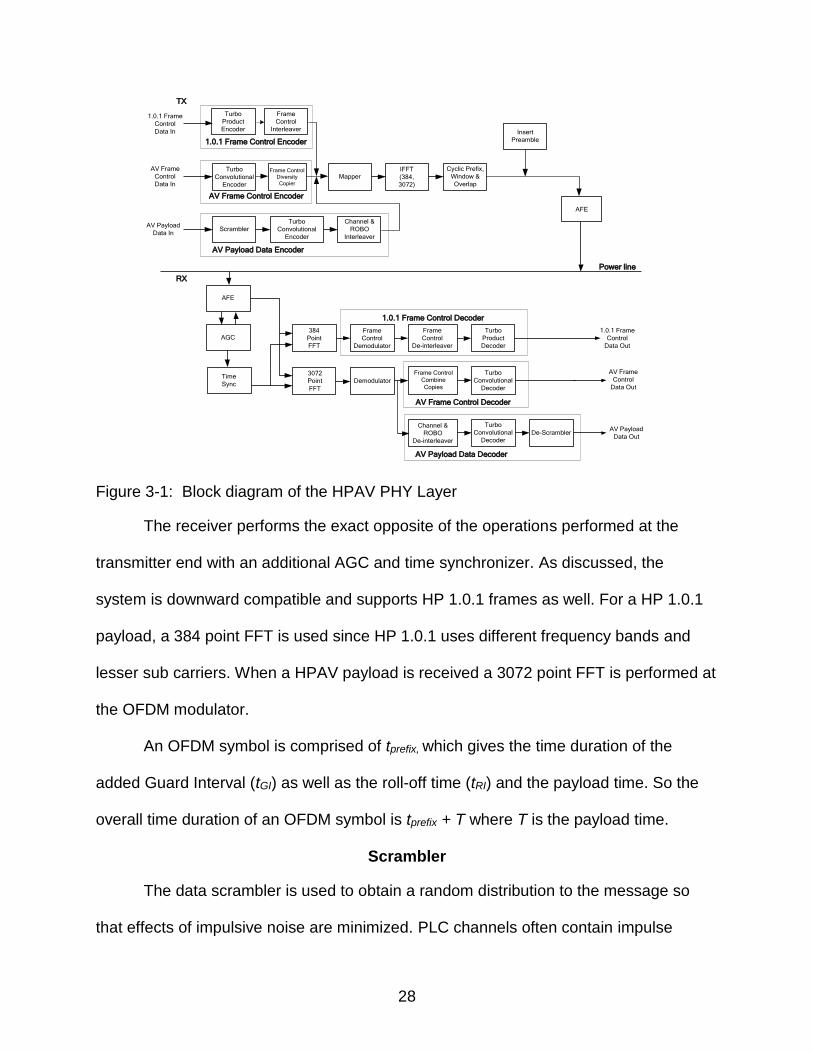
Figure 3-1 shows the basic block diagram of a HPAV communication system [5].

It can be seen that the FEC schemes employed for a HPAV frame and HP1.0.1

are different. As mentioned bore, turbo codes were not used by HomePlug products

before HPAV. In order to provide downward compatibility, provisions are made to

encode HP 1.0.1 frames using a turbo product encoder. The payload however makes

no distinction between the two standards. HPAV systems do not used equalizers

because of the use of conventional FFT OFDM for multi carrier modulation. Since

OFDM divides the spectrum into several ‘flat’ carriers, the equalizer is substituted by an

Automatic Gain Control (AGC) to handle the channel attenuation.

28

1.0.1 Frame Control Encoder

AV Payload Data Encoder

AV Frame Control Encoder

Scrambler

MapperIFFT

(384,

3072)

Turbo

Convolutional

Encoder

Channel &

ROBO

Interleaver

Insert

Preamble

AFE

Power line

Turbo

Convolutional

Encoder

Turbo

Product

Decoder

Turbo

Convolutional

Decoder

Frame

Control

De-interleaver

384

Point

FFT

AGC

Time

Sync

Frame

Control

Demodulator

AFE

Demodulator

Channel &

ROBO

De-interleaver

TX

RX

Turbo

Product

Encoder

AV Payload Data Decoder

1.0.1 Frame Control Decoder

De-Scrambler

3072

Point

FFT

AV Payload

Data Out

Frame

Control

Interleaver

Frame Control

Diversity

Copier

AV Frame Control Decoder

AV Frame

Control

Data Out

Frame Control

Combine

Copies

Cyclic Prefix,

Window &

Overlap

1.0.1 Frame

Control

Data Out

1.0.1 Frame

Control

Data In

AV Frame

Control

Data In

AV Payload

Data In

Turbo

Convolutional

Decoder

Figure 3-1: Block diagram of the HPAV PHY Layer

The receiver performs the exact opposite of the operations performed at the

transmitter end with an additional AGC and time synchronizer. As discussed, the

system is downward compatible and supports HP 1.0.1 frames as well. For a HP 1.0.1

payload, a 384 point FFT is used since HP 1.0.1 uses different frequency bands and

lesser sub carriers. When a HPAV payload is received a 3072 point FFT is performed at

the OFDM modulator.

An OFDM symbol is comprised of tprefix, which gives the time duration of the

added Guard Interval (tGI) as well as the roll-off time (tRI) and the payload time. So the

overall time duration of an OFDM symbol is tprefix + T where T is the payload time.

Scrambler

The data scrambler is used to obtain a random distribution to the message so

that effects of impulsive noise are minimized. PLC channels often contain impulse

29

noises and scrambling avoids the distortion of a single chunk of the message by

distributing the data randomly. The scrambler consists of a series of shift registers or

delay elements which are initialized to either all 0’s or all 1’s and the message bits are

serially input to it. Depending on the scrambler polynomial, the contents of this register

are XOR-ed at different locations and the output message is generated. The scrambler

polynomial used for the simulation is as specified by HPAV specifications.

Turbo Convolutional Encoder

Data from the scrambler is then fed to a turbo convolutional encoder. Turbo

codes are licensed by French telecom and require a patent fee to be paid for every

turbo code enabled manufactured device. Two Recursive Systematic Convolutional

(RSC) constituent codes are used along with a turbo interleaver. These codes support

sizes of 520, 136 and 16 octets. Code rates of 1/2 and 16/21 are available after

puncturing. However, only ½ code rate FEC is used for HAPV when it functions in

ROBO mode since the channel conditions are harsh in such a scenario and more the

number of parity bits, higher is the probability of detecting and correcting errors. But this

also presents additional redundancy.

ROBO Modes

ROBO modes are used under harsh channel conditions. In such cases, “getting

some data is better than getting none” and hence ½ rate codes are used with minimal

loss of efficiency. ROBO modes are also used for several other purposes such as:

Data multicast and broadcast communication

Session setup

Management message exchanges ROBO modes use QPSK for digital modulation and ½ rate codes for FEC as mentioned

above. ROBO interleaver is different from the turbo interleaver since it introduces

30

additional redundancy to improve reliability. With the use of ROBO modes, information

about the use should also be sent to the mapper to update the mapping to ROBO

mode.

Mapping

The mapper decides what digital modulation scheme should be employed on the

data. Based on the modes of transmission and the type of input frame, the mapper

makes its decision. For frame control information, the modulation is always chosen to

be QPSK. When the transmission mode is ROBO, the modulation scheme is again set

to QPSK. For all other payload data, different modulation schemes are chosen based

on the channel conditions. The modulation scheme to be chosen is decided by bit

loading algorithms which monitor the channel conditions and decide the number of bits

to load for every symbol.

The frequency selective nature of Power Line channels results in different OFDM

sub carriers having different attenuations which hinder the achievement of maximum

efficiency with static bit loading over all carriers. By estimating the nature of the channel,

the bit loading can be chosen in such a way that the error rate remains constant while

total number of bits transmitted increases. This helps in obtaining higher data rates

without increase in BER which will eventually result in a greater throughput. Different bit

loading algorithms have been proposed to effectively load bits on to different OFDM sub

carriers such that static error rates are maintained with increase in the raw bit rate. The

state-of-the-art bit loading algorithms are studied in the next chapter and a modified bit

loading algorithm is proposed to best suit HPAV systems.

31

Multicarrier Modulation Using OFDM

Channels such as a PLC channel are highly frequency selective in nature.

Frequency selective channels provide different levels of attenuation at different

frequencies making it tedious for efficient transmission and reception. Hence the

available bandwidth can be divided into various sub channels and data transmission

can be carried out on each of those sub channels simultaneously so that each of these

sub channel have flat fading (constant attenuation across the bandwidth). This is called

Frequency Division Multiplexing (FDM). With each sub channel, a specific sub carrier is

associated (usually, it is the center frequency so that it has equal frequency space on

either side to spread out). The terms sub channel and sub carriers are often

interchangeably used. These sub channels often need to be separated by a certain

frequency called the guard band so that they do not roll off into each other and cause

Inter Carrier Interference (ICI). Orthogonal Frequency Division Multiplexing or OFDM

abolishes the need for this guard band by allowing overlap of adjacent sub channels,

thereby providing better bandwidth efficiency.

Consider a message signal X(f) with data points associated with every ‘f’ and a

carrier signal of frequency fc which can be represented as a complex sinusoid of ei2πfct.

The modulated signal therefore becomes X(f) j2πfct. With ‘n’ such sub carriers, the

eventual modulated signal is

𝑥(𝑡) = ∑ 𝑋(𝑓)𝑒𝑗2𝜋𝑛(𝑓𝑐)𝑡𝑛 (3-1)

This turns out to be the equation for Inverse Discrete Fourier Transform (IDFT)

with a scaling factor. Extracting the message can be done similarly by performing the

32

inverse of it, which is the Discrete Fourier Transform (DFT) of the received signal. The

message signal estimate 𝑋′(𝑓) can be recovered from the received signal 𝑥′(𝑡) using

𝑋′(𝑓) = ∑ 𝑥′(𝑡)𝑒−𝑗2𝜋𝑛(𝑓𝑐)𝑡𝑛 (3-2)

DFT implementation on hardware and in simulations is carried out using efficient

algorithms called Fast Fourier Transform (FFT) and Inverse Fast Fourier Transform

(IFFT). Different FFT algorithms such as Prime Factor Algorithm, Bruun’s Algorithm,

and Rader’s Algorithm etc can be found in [18]. The carrier signal can therefore be

modulated using IFFT and the message can be extracted at the receiver by FFT,

thereby achieving OFDM modulation. Since the sub carriers are all orthogonal to each

other, overlap of sub carriers can be permitted with no loss of information. The FFT and

IFFT equations help in understanding why the overlap of sub carriers can be permitted

without losing any data.

Tone Mask

As seen from the calculations at the beginning of the chapter, there are 1155

available carriers in the 1.8 MHz – 30 MHz of frequency range. But all these carriers

cannot be used for OFDM. FCC regulations prohibit the use of all sub carriers as some

of these interfere with the HAM bands. Tone mask defines the sub carriers that lie in

this region which are required to be notched. These regulations hold well throughout

North America and different regions have various such regulations. Information

regarding carrier notch-outs is held by the Tone Mask and HPAV system provides

support to any kind of Tone Masks depending on the region in which the products are

intended to be marketed.

33

CHAPTER 4 MODIFIED ADAPTIVE BIT LOADING ALGORITHM

Review of Existing Bit Loading Algorithms

Powerline channels typically exhibit frequency selective fading which results in

different OFDM sub carriers suffering different values of attenuation. This results in over

modulation or under modulation when constant bit loading is executed on all sub

carriers. Over modulation is the condition where a bad sub carrier with high attenuation

is given a greater modulation scheme causing high Bit Error Rate (BER) and under

modulation is when a good sub carrier with low attenuation is given a low modulation

scheme resulting in under utilization of the sub carrier. Adaptive Bit Loading (ABL)

exploits this frequency selective fading prevalent in powerline channels to load different

bits/symbol (modulation schemes) on different sub carriers based on the sub channel

SNR. The ABL bit loader is typically present in the ‘Mapper’ block which can be seen in

the general block diagram of a HomePlug AV PHY layer in Figure 3-1.

There are several ABL algorithms which can broadly be classified into two

sections:

1. Adaptive bit loading with adaptive energy profile 2. Adaptive bit loading with constant energy profile

The FCC restrictions levied on powerline communications require the maximum

transmit Power Spectral Density (PSD) in 1.8 – 30 MHz frequency band to be -50

dBm/Hz. This rules out the choice of the first class of ABL algorithms which give an

adaptive power allocation based on the sub carrier SNR. In this class of ABL algorithms,

the data transmitted on sub carriers with high SNRs are allocated low transmit power

and the bit loading is done subsequently. Similarly, the data transmitted on sub carriers

with low SNRs are given higher transmit power and the bit loading is done based on this

34

power allocation. However, in powerline communications this cannot be performed in

this frequency band due to the FCC regulations mentioned above. This limits the choice

of ABL algorithms to the second class of algorithms. The two most widely known ABL

algorithms are considered and it is shown that the Wyglinski-Labeau-Kabal (WLK)

algorithm outperforms the traditional water-filling algorithm. Furthermore, the drawbacks

in a powerline communication system with WLK algorithm are analyzed and a modified-

WLK algorithm is proposed to better suit the HomePlug AV and other powerline

communication systems.

Water Filling Algorithm

The water filling algorithm is a primitive bit loading scheme which chooses the

digital modulation scheme based on the threshold BER. Once the threshold BER is set,

the algorithm tries to select different modulation schemes for different sub carriers to

achieve an average BER which is lesser than the threshold BER. However, it does not

iteratively adapt based on the calculated BER. Once the bit loading scheme is set, it

does not change it until there is a change requested due to either a change in channel

condition or a load change. The BER is calculated from the channel SNR which in turn

is calculated using the channel frequency response using the following relation:

𝑆𝑁𝑅 = 𝜉𝐻.𝐻′

𝜎.𝜎 (4-1)

ξ corresponds to the energy and H corresponds to the PSD of the channel with H’ being

its complex conjugate. σ indicates the noise variance present.

Using this value of SNR, the bit loading scheme is decided using the equation:

𝑏 = 0.5 ∗ log(1 +𝑆𝑁𝑅

Г) (4-2)

35

Г is the SNR gap, which indicates how far the system is away from the maximum

achievable capacity and ‘b’ is the number of bits/symbols loaded on the sub carrier.

Once the bit loading is done, the BER is not computed again to check if a better

loading scheme can be performed. The loading once done is assumed to be the ideal

one. Though the BER obtained from such a scheme will be well within the threshold

BER limit, the bit loading can possibly be improved for certain sub carriers depending

on how far away from the SNR threshold they are.

WLK Algorithm

The WLK algorithm was proposed by Alexander Wyglinski, Fabrice Labeau and

Peter Kabal in July 2005 [19]. This was an adaptive bit loading scheme applicable to

any general multi carrier communication system. The adaptive bit loading is done such

that the resultant BER is smaller than the threshold BER.

The maximum allowable modulation scheme is first chosen for all the available

carriers. In the case of HomePlug AV systems, this is 1024 – QAM. The BER of the

individual sub carriers are then calculated using the theoretical BER estimation

expression [20]. Using these individual BERs, the average BER of all the sub carriers is

calculated and compared with the threshold value. If the value is lesser than the

threshold, the algorithm ends and the bit loading scheme is obtained as 1024 – QAM on

all carriers. However, for powerline channels, this case is highly unlikely. If the average

BER is greater than the threshold value, the sub carrier with the highest BER is

identified and the bit loading is reduced by 2. This implies that the worst sub carrier is

chosen and the modulation scheme of that carrier is lowered. The reduction is done in

steps of 2 as the obtained constellation points are desired to be equidistant. Once the

reduction is done, the average BER is recomputed and compared with the threshold.

36

This process is repeated until the average BER goes below the threshold. In cases

where such a bit loading scheme cannot be achieved, the transmission is done in

HomePlug AV ROBO mode where the bit loading on all sub carriers is set to 2 (i.e.

QPSK on all carriers).

The WLK algorithm is as follows:

1. Initialization: Set the modulation scheme of all the subcarriers to 1024 – QAM.

a) Determine Pi, i = 1, . . . , N, for every sub channel, from the subcarrier SNR values [20], where Pi is the BER for every subcarrier ‘i’ with a constellation size Mi using the relation

𝑃𝑀𝑖,𝑖(Г𝑖) = 4 (1 −1

√𝑀𝑖) 𝑄 (√

3Г𝑖

𝑀𝑖−1) [1 − (1 −

1

√𝑀𝑖) 𝑄 (√

3Г𝑖

𝑀𝑖−1)] (4-3)

For a BPSK modulation,

𝑃2,𝑖 = 𝑄(√2Г𝑖) (4-4)

Where Г(𝑖) is the SNR of the i-th sub-channel.

2. Compute weighted average P using the expression:

𝑃 = ∑ 𝑏𝑖

𝑁𝑖=1 𝑃𝑖

∑ 𝑏𝑖𝑁𝑖=1

(4-5)

where N = total subcarriers

3. Compare with the threshold BER. If P < threshold BER, configuration is retained and the algorithm ends.

4. Search for the subcarrier with the worst Pi and reduce the bit loading by 2. If bi = 1, null the subcarrier (i.e., set bi = 0), where bi is the number of bits/symbol loaded in every subcarrier ‘i’

5. Recompute Pi of all subcarriers with changed allocations and return to Step 3.

Drawbacks for PLC Implementation

The WLK algorithm works as expected for a clean wireless channel which can be

modeled as a channel with AWGN. However, it cannot be directly incorporated into a

powerline communication system. The calculation of BER from the sub carrier SNR as

shown in (4-3) and [20], holds true only when the noise present in the entire

37

communication system is limited to AWGN. A powerline channel noise, however, is

characterized by high attenuation, multipath, random impulsive noise and frequency

selective fading [2]. This makes it impractical to use the WLK algorithm for powerline

communication systems.

Modified Adaptive Modulation Algorithm

A modification to the WLK algorithm is proposed such that it can be used

effectively for powerline systems. The drawback that was identified was the exclusive

consideration of AWGN noise in the estimation of the sub carrier BER. This can be

addressed by including the powerline noise effects that are present in the system. It can

be accomplished in two ways:

1. The BER v/s SNR curves can be obtained for a typical HomePlug AV system by building the PHY layer of the system. The procedure is explained in later sections. From this plot, a Look-Up Table (LUT) can be generated to get different values of BER and SNR for a particular channel. For simulation simplicity, a new expression relating the BER and the SNR can be determined. This expression or the LUT can be used to ascertain the bit loading estimate in all the iterations.

2. The second way of achieving this is by accommodating the powerline noise while determining the value of SNR. The determination of SNR in the WLK algorithm is done by considering the ratio of the signal power and the AWGN noise power. In this expression, the powerline noise power can also be added such that the resultant SNR includes the effect of the powerline noise present.

In this simulation study, the second approach is chosen as it possesses lesser

implementation complexity. The rest of the algorithm remains the same, as explained in

the previous section.

Simulation Results and Performance Evaluation

The primary step in evaluating the performance of ABL algorithms is to build a

basic HomePlug AV communication system, the block diagram of which is shown in

Figure 3-1. Ten different powerline channels and their corresponding noise samples

38

were provided by Qualcomm Atheros [8]. The impulse responses of the channels and

their noise samples were captured inside a house in a powerline circuit connected to

various home appliances such as refrigerator, television, electric lamps, microwave

oven, coffee makers and personal computers. The LUT of BER and SNR values are

obtained by simulating the PHY layer model of Figure 3-1. The simulation environment

and implementation procedure is explained in Chapter 6. This can also be substituted

by following the second procedure of implementation explained in the previous section.

The ABL algorithms are implemented using the algorithms that were explained in the

previous three sections. The performance evaluation is done in terms of data rates

obtained.

In an OFDM transmission, the symbol period is equal to the inverse of the

frequency spacing of the orthogonal sub carriers [21] to maintain orthogonality. With the

available 917 carriers for data transmission, the data rate is calculated as follows:

Data Rate = 917 * m * 24414 bps (4-6)

In this expression, ‘m’ represents the number of bits/symbol used, which is

dependent on the number of bits loaded by the ABL algorithm. The highest modulation

scheme that HomePlug AV can support is 1024 – QAM, for which, m = 10. With this

value, we get the Data Rate = 917*10*24414 = 220 Mbps. This is the theoretical

maximum raw data rate that HomePlug AV systems can provide. With the help of this

equation we can evaluate the performance of the three different ABL algorithms.

For a given channel (Channel 5 shown in Chapter 6) and a static BER of 10-2, the

following bit allocation is obtained using the water filling algorithm.

39

Figure 4-1: Bit loading profile using water filling algorithm

It can be seen that the water filling algorithm chooses only the modulation

schemes of 16 – QAM and QPSK to achieve the required BER for this channel. The

data rate obtained for this scenario was 34.44 Mbps. Figure 3 also shows the frequency

response of the channel after the transmit mask is applied.

The bit allocation obtained by the WLK algorithm with the same simulation

environment is shown in Figure 4-2.

40

Figure 4-2: Bit loading profile using WLK algorithm

It chooses 256 – QAM and 64 – QAM for modulation depending on the sub

carrier SNR. The data rate obtained was 89.7 Mbps. It can be noticed that the data rate

has almost doubled when compared to water filling algorithm. However, this does not

imply that the eventual throughput is also doubled since the efficiency drops as the data

rate increases when no action is taken at higher layers. To make best use of the

increase in Physical layer data rates, care should be taken to maximize the length of the

PHY payload in the MAC layer to make sure the efficiency does not drop with increase

in data rates. Higher layers should also take appropriate measures to make sure

efficiency does not drop so that the increase in PHY data rate can be effectively

reflected in the eventual throughput.

41

The proposed modified WLK algorithm, for the same channel conditions and

error rates, gives the following bit allocation:

Figure 4-3: Bit loading profile using modified WLK algorithm

The data rate obtained in this case was 49.39 Mbps. Though the bit loading

profile is not as large as WLK, this provides a better estimate for the given powerline

communication system since it considers the powerline noise and the channel

attenuation present in the powerline channel. Though the WLK algorithm outperforms

the proposed algorithm, the bit loading profile obtained from the WLK algorithm is an

erroneous one which can be accepted for only a system with AWGN environment.

However, it can be noticed that the data rate obtained is higher than the water filling

algorithm’s data rate.

42

The three different algorithms are simulated for all the 10 powerline channels (to

be seen in Chapter 6) with three different un-encoded BER values of 0.1, 0.01 and

0.001. The data rates (in Mbps) obtained in all these cases are tabulated in Table-1.

Table 4-1: Data rates for different algorithms and error rates

BER = 0.1 BER = 0.01 BER = 0.001

WF M-WLK WF M-WLK WF M-WLK

Channel 1 80.91 117.8 34.90 51.85 29.60 45.38

Channel 2 80.86 110.9 34.72 49.48 29.56 44.75

Channel 3 80.86 111.4 34.84 49.63 29.56 44.75

Channel 4 80.86 111.1 34.79 49.53 29.56 44.75

Channel 5 80.86 110.6 34.44 49.39 29.56 44.70

Channel 6 80.86 110.8 34.44 49.44 29.56 44.76

Channel 7 80.86 110.7 34.44 49.44 29.56 44.70

Channel 8 80.86 110.7 34.44 49.39 29.56 44.70

Channel 9 80.86 111.6 34.84 49.37 29.56 44.80

Channel 10 80.86 111.4 34.84 49.39 29.56 44.75

43

CHAPTER 5 LDPC AND TURBO CODES WITH REAL POWERLINE NOISE

LDPC System Implementation

The encoding procedure for LDPC is discussed in Chapter 2. The encoding is

done based on the Tanner graphs and every v-node generates a code based on the c-

nodes connected to it. For decoding, the widely used iterative decoding algorithm called

Sum-Product Algorithm (SPA) is used. It is used to iteratively update the information of

the c-node and the v-node. A-posteriori probability (APP) is applied for decision making

and the log-likelihood ratio is given by

𝐿 (𝑣𝑗

𝑦) = log (

𝑃(𝑣𝑗 = 0|𝒚)

𝑃(𝑣𝑗 = 1|𝒚)) (5-1)

where y is the received word.

The position of LDPC encoder can be determined by observing Figure 3-1. The

turbo encoder used in a traditional HPAV system needs to be replaced by an LDPC

encoder. The system of turbo encoder and the set of interleaver blocks are replaced by

the LDPC encoder which is built. The rest of the system model remains the same and

similar changes are made at the receiver. The Turbo decoder and the set of de-

interleaver blocks are replaced by the corresponding LDPC decoder.

Turbo Encoding and Decoding

There are two structures of turbo codes that are present:

Parallel Concatenated Convolutional Codes (PCCC)

Serial Concatenated Convolutional Codes (SCCC)

Based on the choice of HPAV and IEEE 1901 [2], the PCCC is incorporated in the

simulations for encoding using the turbo codes. Turbo codes are essentially two or more

convolutional encoders connected with a pseudo-random interleaver. The encoder is

44

configured with RSC encoders as discussed in Chapter 2 with an N-bit pseudo-random

interleaver. Generally, the two RSC encoders used are similar to each other, i.e., have

the same generator polynomial functions.

For the decoding of turbo codes, the iterative soft decision algorithm is used. The

Bahl-Cocke-Jelinek-Raviv (BCJR) algorithm [22] is applied for the decoding process

using the Maximum A-posteriori Probability (MAP), which is done iteratively.

Performance Evaluation of LDPC and Turbo Codes With Real Powerline Noise

The performance evaluation of LDPC and Turbo codes are carried out with

LDPC codes of different block lengths of 256, 512 and 1024 along with a turbo coded

system and a system with no FEC. The simulations are carried out with real powerline

noise samples provided by Qualcomm Atheros. The noise samples are as shown below

in Figure 5-1.

It can be seen from the noise samples that the powerline noise is characterized

by impulse noise, phase noise, transient noise and other type of noise. The 10 different

noise samples captured all the variants of noise possible in a powerline. For example,

noise present in Channel 7 contains consistent impulse noise possible due to the use of

equipment such as a hair dryer. On the other hand, nearly constant but high amplitude

noise is present in Channel 1. Noise present in Channel 6 for example, is constant and

low amplitude and possibly easier to mitigate.

Efficient error correction should be employed to make sure these noise values do

not have adverse affect on the transmitted data.

45

Figure 5-1: Noise samples seen on powerline channels

The PCCC turbo encoders are simulated based on the choice made by HPAV

and IEEE 1901 standards. The LDPC encoder and decoder are implemented as

discussed in Chapter 2. The BER simulation result for the system is shown in Figure 5-

2.

46

Figure 5-2: Error rate performance of LDPC and Turbo codes under powerline noise environment

It can be seen that although the turbo codes perform slightly better than LDPC

codes at low SNRs, the LDPC codes begin to outperform as the signal power increases.

Also, it can be seen that the LDPC codes with higher block lengths are higher

performance codes as compared to the smaller block length ones.

This serves as a motivation to evaluate the performance of LDPC codes with

high block lengths for a standard HPAV system and examine if it can serve as a viable

alternative to the licensed turbo codes that are in use in the current HPAV products. But

the complexity of implementation and the requirement of memory increases with

increase in block lengths. This can be addressed by using Quasi Cyclic – LDPC (QC-

LDPC) codes.

47

The next chapter discusses the implementation of a HPAV system model and the

use of LDPC codes as FEC for such a system. The performance of the system with high

block lengths of LDPC codes for FEC is compared to a traditional HPAV system with

turbo codes.

48

CHAPTER 6 LDPC AND TURBO CODES ON A REAL POWERLINE CHANNEL AND HOMEPLUG

AV STANDARDS

The block diagram of a standard HPAV system is shown in Figure 3-1. The AV

payload entering from the MAC layer passes through the scrambler, defined in the

HPAV specifications, and then enters the turbo encoder and interleaver blocks. The

turbo codes provide the necessary FEC for the system and are traditionally known to

provide better error rates than LDPC codes at low SNRs. This is also seen in [17] and

Figure 5-2. However, Figure 5-2 also reveals that LDPC codes begin perform better as

the block length increases. This serves as a motivation to investigate if LDPC codes

with sufficient block lengths can provide better error performance when compared to

turbo codes. Successful implementation of such a system would provide an alternative

to the licensed turbo codes which require a patent fee to be paid for every turbo code

enable device.

The increase in block length of LDPC codes is accompanied by two major

obstacles:

Increase in implementation complexity

Increase in memory requirement Both these issues can be addressed with the use of QC-LDPC codes, which

provide a simpler implementation structure in terms of generation of the parity check

matrix and the generator matrix. The memory required is also substantially reduced

since matrices are formed by permutations of a base matrix, explained in detail in the

next chapter.

49

Encoding and Decoding Process for LDPC

The process of encoding and decoding using LDPC codes are explained in

Chapter 2 and in Chapter 5. Similar steps are followed for a HPAV system model. The

data scrambled by the pseudo random scrambler is passed through the LDPC encoder.

The block length of the encoder is decided based on the error rate performance

required. In Figure 5-2 it can been seen that, although the LDPC codes of block length

8640 perform better than turbo codes at high SNRs, the additional complexity of LDPC

codes are being wasted at low SNRs, common for long propagation runs of powerline

channels, where the simpler-to-implement turbo codes still outperform their LDPC

counterparts. This forces the use of LDPC codes of higher block length. For simulation

purposes, a quantum leap in the block length of LDPC codes is employed and a 32400

sized LDPC code is used for initial simulation. Unlike convolutional coding where the

data is encoded serially, LDPC codes are block codes which require the data to be

buffered until the block length is satisfied. This places a memory requirement overhead

and the overhead increases with increase in block lengths. Depending on the

performance of this system, the block lengths can further be reduced or increased. The

parity check matrix is first built based on the message bits and the corresponding code

word to be generated. The encoding procedure is explained in Chapter 2 and is

graphically shown in Figure 2-1.

At the receiver, the signal, after demodulation, is admitted in to the LDPC

decoder. The parity check matrix, H, should also be stored at the decoder since every

row of H is associated to every c-node and columns with the v-nodes. The iterative

decoding algorithm, SPA is used for decoding. At the decoder, based on the signal that

the v-nodes receive, it sends information to the connected c-nodes. Messages from all

50

v-nodes are collected and the c-nodes estimate based on the information it gets from all

v-nodes it is connected to. These estimates are sent back to the corresponding v-

nodes. The information sent from one c-node to a v-node is based on the information

that the c-node receives from all other v-nodes except the one that it is sending the

estimate to. One set of message and estimate exchange between the c-node and v-

nodes forms one iteration. These iterations continue until the correct codeword is

estimated or until the maximum number of iterations is reached. At the end of the

iterations, a codeword is finally estimated.

Simulation Environment and System Implementation

System Parameters Specified by HPAV

Simulation constants for a HPAV system are the system parameters that are

defined in the HPAV specifications.

Sampling Frequency: The sampling frequency used throughout the system is 75 MHz and is especially required to interpret the channel transfer function from the impulse response.

FFT Size: The FFT size used by HPAV systems is 3072. These are the total number of carriers available for OFDM multicarrier modulation, but include the frequencies in the negative spectrum as well. This divides the available spectrum into 3072 equally space orthogonal sub carriers.

Sub carrier size: This value contains the total number of sub carriers that are used for data modulation. Out of the 3072 total carriers, half of them lie in the negative spectrum. Hence the total useful carriers are 1536. However, only 1155 of these lie in the bandwidth (1.8 MHz – 30 MHz) available for HPAV operation. Of these, there are carriers which lie in the HAM bands and are required by the FCC regulations to be notched out. Hence for North America, the total useful sub carriers available for data transmission are 917.

Bits per OFDM symbol: One OFDM symbol is the total number of symbols on each of the OFDM sub carriers. Since there are 917 sub carriers that are used, there are 917 symbols per OFDM symbol for the primitive case of BPSK modulation. When higher modulation schemes are used, this number would increase based on the bit loading used.

51

Sub carrier spacing: Based on the FFT size and the sampling frequency the sub carrier spacing can be evaluated. The 3072 – point FFT provides 3072 equally spaced carriers in a bandwidth if 75 MHz; hence the sub carrier spacing would be 75 MHz / 3072 = 24.414 kHz.

Symbol duration: For the OFDM sub carriers to preserve orthogonality, the sub carrier spacing should be equal to the inverse of the symbol duration. Consider two carriers of frequencies f1 and f2. For them to be orthogonal to each other,

∫ cos(2𝜋𝑓1𝑡 + 𝛼) cos(2𝜋𝑓2𝑡) 𝑑𝑡 = 0 (6-1)

α is the phase difference between the signals and the integral is over the time

period T, which is also the symbol duration. Assuming (𝑓1 + 𝑓2)𝑇 to be an integer, the solution of the integral simplifies to

cos(𝛼)sin (2𝜋(𝑓1−𝑓2)𝑇)

2𝜋(𝑓1−𝑓2)+ sin(𝛼)

cos(2𝜋(𝑓1−𝑓2)𝑇)−1

2𝜋(𝑓1−𝑓2)= 0 (6-2)

The solution of this equation requires, 2𝜋(𝑓1 − 𝑓2)𝑇 = 2𝑘𝜋, where k is any positive

integer. The minimum value of k is 1 and hence we get the condition, 𝑓1 − 𝑓2 =1

𝑇.

This gives the frequency spacing of 1/24.414 kHz = 40.96 us.

Carriers in the HAM band: FCC regulations require certain carriers in the 1.8 MHz – 30 MHz band to be notched off so that they do not interfere with the amateur carriers. These notching often require certain guard bands as well, to make sure there is no carrier roll-off. Windowed OFDM provides deep notches which remove the requirement of use of complex band stop filters. The information about these carriers that required to be notched off is stored in this field.

Scrambler polynomial: The scrambler polynomial is stored as a 1-D vector containing a set of 1’s and 0’s. When a shift register is connected to the adder, the corresponding bit in the scrambler polynomial vector is turned to ‘1’. All the remaining bits are kept at ‘0’.

Scrambler initialization: The scrambler is usually initialized to either all 1’s or all 0’s. However, if there is a change in the initial state required, it is modified accordingly.

Modulation order: This chooses the bit loading that is performed on the different sub carriers based on the channel conditions. Based on the bit loading scheme given by the adaptive bit loading algorithm, the modulation order is set. Different modulation order is set for different sub carriers based on the attenuation present in that sub carrier. OFDM aids in viewing every sub channel as a flat fading channel even though the spectrum shows a frequency selective nature the powerline channel. The channel condition is fed to the adaptive bit loading algorithm based on the ‘SOUND’ packets that are sent at regular intervals.

52

Whenever there is a change in the channel condition, the adaptive bit loading algorithm gives a new bit loading scheme which changes the modulation order of the different sub carriers.

Implementation of Forward Error Correction Coding

Based on the FEC scheme that is employed, a turbo or an LDPC encoder block

is built. For an LDPC encoder, the parity check matrix is used, the generation of which

is explained in Chapter 2. The encoder builds a generator matrix for the parity check

matrix that it receives. The parity check matrix is formed based on the block length and

the code rate that is required. For simulation purposes, the message that needs to be

transmitted is generated as a random set of equally likely 1’s and 0’s. This data is then

multiplied with the generator matrix constructed by the LDPC encoder.

For a system with turbo codes as FEC, the message bits are passed through the

turbo encoders and interleaver built as discussed in Chapter 5. The same turbo encoder

is used in a HPAV system as well.

For the LDPC encoder the message bits enter a buffer serially and are grouped

into initial blocks of length 32400. The block length can then be varied based on the

robustness required. The message is then supplied serially to the digital modulator.

Digital Modulation

The modulator operates on the signal based on the modulation scheme chosen

by the modified adaptive bit loading algorithm developed and studied in Chapter 4. The

bit loading algorithm provides modulation schemes for all sub carriers based on the

individual sub channel SNR. The message data is divided into several groups of 917

bits each. Each of these 917 bits is further loaded on to the available 917 sub carriers at

the OFDM modulator.

53

Carrier Notching for FCC Compliance

As per FCC regulations 238 out of the available 1155 carriers in the range 1.8

MHz – 20 MHz are notched off and the remaining 917 carriers are loaded with blocks of

data divided into various blocks of length 917 each.

OFDM

OFDM is used for multicarrier modulation as the 917 bits in each block are

loaded on to the 917 available carriers using IDFT. This is accomplished on hardware

and simulations using one of the FFT algorithms discussed in Chapter 2.

Guard Intervals (GI)

OFDM requires GI to be prefixed before every symbol in each of the 917 carriers

to prevent or reduce Inter Symbol Interference (ISI). The size of GI to be added is

dependent on the channel impulse response. Ideally, the GI should be greater than the

delay spread of the channel so that the adjacent symbols do not ‘spread’ on each other.

The length of GI is also dependent on the type of information being sent. For payload

data lesser GI is used and for frame control data, higher length GIs are used. For

OFDM, the GI is the last few bits which are prefixed to the beginning of an OFDM

symbol to make sure the circular convolution in DFT still holds valid and is hence called

cyclic prefix (CP).

Signal Power

The maximum allowable signal power spectral density (PSD) for transmission

over powerlines in the given frequency range is also specified by the FCC to be -

50dBm/Hz. It should ensured that the generated signal has a PSD lesser than or equal

to this value.

54

Receiver

The exact opposite processes are carried out at the receiver to recover the

message signal. The GIs are removed based on the data that is being processed. The

GI lengths are higher for frame control data and are generally lesser for regular payload

data. OFDM de-modulation is performed using one of the FFT algorithms mentioned in

Chapter 3. The OFDM de-modulation expression is shown in (3-2). The data on the

orthogonal sub carriers are extracted using FFT. Based on the Tone Mask, the data is

obtained from the corresponding carriers by ignoring the notched out carriers in the

amateur radio band. The data is then demodulated using the bit allocation provided by

the adaptive bit loading algorithm and is then sent to a decoder block. The decoder is

either an LDPC decoder which uses the SPA for decoding or a standard turbo decoder

used in HPAV systems. The message recovered is then compared to the originally

generated message to check the error rates.

PLC Channel and Noise Effects

For this simulation 10 different powerline channels and their corresponding noise

values are considered. The impulse responses and noise samples were captured on a

real powerline circuit connected to various appliances such as electric lamps, coffee

makers, televisions, refrigerator, microwave oven and personal computers.

Figure 6-1 shows the network configuration with 5 nodes and 10 different

channels. The five nodes A, B, C, D and E are access points inside the house.

55

Figure 6-1: PLC network configuration for channel measurement

The 10 different noise samples that were used are shown in Figure 5-1. It can be

seen that most of the channels are characterized by impulse and various other types of

noises, thereby making it a very harsh communication channel. The impulse responses

and the frequency responses of the channels are shown in Figure 6-2 and Figure 6-3

respectively.

It can be observed from Figure 6-3 that all the powerline channels are frequency

selective in nature and the use of OFDM is quintessential for the successful

transmission of data. Figure 6-2 shows the high latency and delay spread associated

with each of the powerline channels.

56

Figure 6-2: Impulse responses of the PLC channels

57

Figure 6-3: Frequency responses of the PLC channels

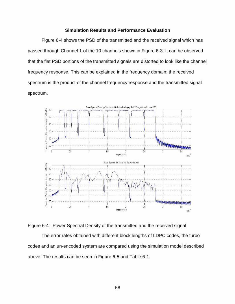
58

Simulation Results and Performance Evaluation

Figure 6-4 shows the PSD of the transmitted and the received signal which has

passed through Channel 1 of the 10 channels shown in Figure 6-3. It can be observed

that the flat PSD portions of the transmitted signals are distorted to look like the channel

frequency response. This can be explained in the frequency domain; the received

spectrum is the product of the channel frequency response and the transmitted signal

spectrum.

Figure 6-4: Power Spectral Density of the transmitted and the received signal

The error rates obtained with different block lengths of LDPC codes, the turbo

codes and an un-encoded system are compared using the simulation model described

above. The results can be seen in Figure 6-5 and Table 6-1.

59

`

Figure 6-5: BER performance of LDPC and Turbo codes on a real powerline channel

Table 6-1: Error rates for different FEC schemes

SNR (dB) 0 1 2 3 4 5 6

Un-encoded 0.07496 0.03282 0.01981 0.00498 0.000817 0.000117 0 Turbo, Rate ½

0.07413 0.0300 0.00718 0.00113 0.00012 3.26e-06 0

LDPC – 16200, Rate ½

0.07465 0.03549 0.01475 0.00186 4.13e-05 0 0

LDPC 32400, Rate ½

0.07465 0.02169 0.00466 0.00054 0 0 0

The simulation results support the theory that the turbo codes provide better error

rates as opposed to low block length LDPC codes at low SNRs. The LDPC-16200, rate

½ codes cross over the turbo code, rate ½ curves at 3 dB until which the turbo codes

perform better; after which, the LDPC-16200 rate ½ codes provide 65% improvement in

60

error rates at 4 dB and a sharp decline in the curve from there on. However, the biggest

outcome from these results is the error rates of the LDPC codes with high block length

(32,400). The error rates of these are consistently better than the ones provided by the

system with turbo codes. Even at low SNRs of 1 dB, LDPC – 32400 rate ½ codes

provide 28% decrease in error rates when compared to turbo codes, followed by a

steep decline as SNRs improve further.

However, increase in block length is accompanied with increase in

implementation complexity and memory requirement. This encourages the need to

investigate better implementation of LDPC codes to reduce the complexity and memory

required.

61

CHAPTER 7 QUASI CYCLIC – LOW DENSITY PARITY CHECK CODES (QC-LDPC)

An (n, k) Quasi Cyclic (QC) code Cqc is a linear block code over GF(2)

when n = t*b, where b, t and k are positive integers with the constraint k < tb.

There are two conditions levied on every QC code.

Every codeword should contain t sections of b bits each

After a cyclic shift in Cqc, every code word should be another new codeword in Cqc [23]

In order to produce efficient QC-LDPC codes, two methods based on

circulant permutation matrices and finite geometries are investigated in [24], [25]

and [26]. The parity check matrices for these codes can be obtained by using

circulant permutation of a base matrix. Hence the parity check matrix, H, can be

obtained by column permutation of a permutation matrix which is initially defined.

This provides a major advantage for the QC-LDPC codes over randomly

generated LDPC codes. Since H can be generated by permutations of a base

matrix, the memory requirement is reduced. Also, the permutation

implementation is simpler than the complex LDPC parity check matrix that is to

be built.

For QC-LDPC encoding, consider a base permutation matrix P of order

qxq. The parity check matrix H is generated by the circulant permutations of P. It

requires the term q to be a prime number [27]. The first row of H is first filled and

the remaining rows are filled based on the permutations of P. Hence it can be

seen that the memory requirement is greatly reduced and the complexity of

building H is also simplified.

62

For the decoding process either the SPA or a Bit-Flipping Algorithm (BFA)

can be used. BFA is a hard decision decoding unlike the SPA. The parity check

matrix H and the received vector y are considered and the term H.yT is

computed. The non-zero elements in this new computed vector are identified.

After every bit node resolves the c-nodes, the largest number of the unsatisfied

c-nodes is found out. The bits of y involving this c-node are all ‘flipped’. All the 1’s

in the vector are turned to 0’s and the 0’s into 1’s. This process is carried on until

the term H.yT = 0 or until the maximum number of iterations is reached. But

during this process, some of the bits which were rightly estimated might also be

flipped. To avoid this, [28] proposed that only one bit should be flipped in every

iteration. But this increases the number of iterations to get acceptable results.

Based on these factors either of the two decoding algorithms has to be

chosen for effective decoding. Thus, QC-LDPC codes provide simpler

implantation of LDPC codes and also reduce the memory requirement. This

enables the use of high block lengths LDPC codes for HPAV systems.

63

CHAPTER 8 CONCLUSIONS AND FUTURE WORK

The adaptive bit loading and FEC schemes of a traditional HPAV system were

modified in the course of this work to obtain higher bit rates and lower error rates

respectively. The adaptive modulation scheme currently used by HPAV system decides

the bit loading scheme based on the channel SNR and adaptively modulates every sub

carrier correspondingly, in a single shot. However, the proposed adaptive bit loading

algorithm iteratively updates the bit loading on each of the sub carriers to reach an

optimum bit loading such that the data rates are maximized under a threshold error rate.

Simulation results indicated a 43% improvement in data rates from 34.44 Mbps to 49.39

Mbps for a real powerline channel with a threshold un-encoded BER of 10-2.

Adaptive bit loading can be better appreciated and tested when the channel

conditions are continuously changing, such as a real world PLC channel. Such a system

model can be simulated to test the performance of different adaptive modulation

algorithms. The proposed bit loading scheme requires a significant number of iterations

before it provides the optimum bit loading profile. Future work can involve reducing the

number of iterations by choosing a lower starting point instead of the 1024-QAM chosen

for HPAV systems. The algorithm can start from the profile provided by the water filling

algorithm and then proceed to optimize the bit loading scheme. This can significantly

reduce the number of iterations and the algorithm converges faster.

The BER performance of a conventional HPAV system was also compared with

that of a modified HPAV system with LDPC encoding scheme. The choice of turbo

codes for HPAV and IEEE 1901 standards was because of their effective error rate

performance at low SNRs. The simulations results showed that rate ½ turbo codes

64

outperform rate ½ LDPC codes with block length of 16200 at low SNRs of less than

3dB. However, with increase in block length to 32400, rate ½ LDPC codes provide 28%

lower error rates even at a low SNR of 1 dB.

LDPC codes of high block lengths also present additional implementation

complexity and memory requirement. A rate ½, 32,400 block length LDPC code, for

example, requires storage of parity check matrices of the order 32400X16200. Such

high memory requirements and implementation complexities are addressed by QC-

LDPC codes which provide an efficient parity check matrix generation scheme using

cyclic permutations of a base permutation matrix.

With the use of LDPC codes of high block lengths, the BER was reduced by 28%

when compared to a turbo coded HPAV system even at SNRs as low as 1 dB. This

presented LDPC as a viable alternative for the licensed turbo codes for HPAV systems.

Future research would include implementing this system across all products of HPA

including HPAV2 and HPGP. Although HPGP provides data rates sufficiently larger than

the current smart grid requirements, LDPC codes present an open source alternative to

the existing turbo codes.

For simulation purposes, QC-LDPC and regular LDPC codes provide similar

results. However, the implementation simplicity and lower memory requirement can be

greatly appreciated by developing hardware for such an encoder-decoder system.

Future research could include hardware development for a QC-LDPC enabled HPAV

system.

LDPC encoded HPAV systems would present a compatibility issue with the

already existing turbo code enabled HomePlug products. This requires a design of an

65

Inter System Protocol which would provide interoperability between the HomePlug

products with the two different FECs.

66

LIST OF REFERENCES

[1] H. C. Ferreira, L. Lampe, J. Newbury, T. G. Swart, Power Line Communications: Theory and Applications for Narrowband and Broadband over Power Lines, John Wiley & Sons, West Sussex, UK, 2010

[2] H. A. Latchman, S. Katar, L. W. Yonge III, S. Gavette, HomePlug AV and IEEE 1901 – A Handbook for PLC Designers and Users, 1st ed, IEEE Press, NJ, 2003

[3] “HomePlug Green PHY White Paper”, http://www.homeplug.org

[4] “HomePlug 1.0 White Paper”, http://www.homeplug.org

[5] “HomePlug AV White Paper”, http://www.homeplug.org

[6] Simon Haykin, “Digital Communications”, Wiley, 1988.

[7] C. Hsu, N. Wang, W. Chan, P. Jain, “Improving HomePlug Power Line

Communications with LDPC coded OFDM”, International Telecommunications Energy Conference, 2006, Providence, RI.

[8] “Qualcomm Atheros”, www.atheros.com

[9] “HomePlug AV2 White Paper”, http://www.homeplug.org

[10] J. Costello, G. D. Forney, “Channel coding: The Road to Channel Capacity”, Proc of the IEEE, Vol. 95, pp. 1150-1177, June 2007

[11] Gallager, R. G., Low Density Parity Check Codes, Monograph, M.I.T. Press, 1963

[12] R. M. Tanner, “A Recursive Approach to Low Complexity Codes”, IEEE Trans. Inform. Theory, vol. IT-27, pp. 533-547, Sept 1981

[13] C. Hsu, N. Wang, W. Chan, P. Jain, “Improving HomePlug Power Line Communications with LDPC Coded OFDM”, International Telecommuncations Energy Conference, pp 1-7, Sept 2006

[14] T. Wada, “A Study on Performance of LDPC Codes on Power Line Communication Systems”, Proc. IEEE ISPLC, Jeju, Korea, pp 394-399, Apr. 2008

[15] S. Galli, “On the Fair Comaprison of FEC Schemes”, Proc. IEEE International Conf. Comm., pp 1-6, May 2010

[16] P. Jagatheeswari, M. Rajaram, “Performance Comparison of LDPC and Turbo

Codes”, European Journal of Scientific Research, Vol. 54, No. 3, pp 465-472, 2011

67

[17] G. Prasad, H. A. Latchman, Y. Lee, W. A. Finamore, “A Comparative Performance Study of LDPC and Turbo Codes for Realistic PLC Channels”, International Symposium on Power Line Communications, April 2014

[18] J. G. Proakis, D. G. Manolakis, “Digital Signal Processing”, Pearson, 2007

[19] A. M. Wyglinski, F. Labeau, P. Kabal, “Bit Loading with BER-Constraint for

Multicarrier Systems”, IEEE Transactions on Wireless Communications, Vol 4, No. 4, July 2005

[20] J. G. Proakis, Digital Communications, 3rd ed. New York: McGraw-Hill, 1995

[21] Understanding an OFDM Transmission,

http://www.dsplog.com/2008/02/03/understanding-an-ofdm-transmission

[22] S. Benedetto and, E. Biglieri, “Principles of Digital Transmission”, Kluwer Academic, New York, NY, 1999

[23] W. Ryan, S. Lin, “Channel Codes: Classical and Modern”, Cambridge University

Press, 2009.

[24] Y. Kou, S. Lin, M. Fossorier, “Low Density Parity Check Codes on Finite Geometries: a Rediscovery and New Results”, IEEE Trans. Inform. Theory, Vol. 47, pp. 2711-2736, 2001

[25] R. M. Tanner, D. Sridhara, A. Sridharan, T. E. Fuja, D. J. Costello, “LDPC block

and convolutional codes based on circulant matrices”, IEEE Trans. Inform. Theory, Vol 50, No. 12, pp. 2966-2984, 2004

[26] M. Fossorier, “Quasi-Cyclic Low Density Parity Check Codes from Circulant

Matrices, IEEE Trans. Inform. Theory, Vol. 50, pp. 1788-1794, 2004

[27] Y. Lee, “Conquering the Harsh PLC Channel with QC-LDPC Codes to Enable QoS Guaranteed Multimedia Home Networks”, Ph.D dissertation, Dept. ECE, Univ. of Florida, Gainesville, FL, 2013

68

BIOGRAPHICAL SKETCH

Gautham Prasad completed his Bachelor of Engineering at the Visvesvaraya

Technological University, Belgaum, India from the Department of Electronics and

Communication Engineering in 2012. He obtained his Master of Science degree at the

University of Florida, Gainesville from the Department of Electrical and Computer

Engineering in 2014. His current research interests are smart grids and high speed data

communication over power lines.