Embed Size (px)
Citation preview

2012 اب 18 مجلد 8 العدد مجلة الهندسة
151
األهداف اتخاذ القرارات ذات الدوال الكسرية باستخدام طريقة برمجة
م واثق حياوي اليذ.م
قسم اإلحصاء/كلية اإلدارة واالقتصاد / جامعة ذي قار / هندسة صناعية
-:الخالصة
واإلنتـاج أن عملية صنع القرار من المواضيع المهمة والحيوية في مجال بحوث العمليات والهندسة وعلم االقتـصاد
نها تـساهم ألوذلك في أي منشأة أو منظمة صناعية أو خدمية دارية إلعملية صنع القرار هي جوهر العملية ا وعلم اإلدارة وأن
ارية بكفاءة وفعالية وبالشكل الذي يحقق االسـتغالل األمثـل لمـوارد دإل ا من مزاولة أنشطتها ةدارإل في تمكين ا أساسيبشكل
عملية اتخاذ القرارات عندما تكون دالة الهدف عبارة عن دالة كسرية ، وتم حل نماذج البرمجـة ول البحث تنا .المنشأة المتاحة
win( الكسرية باستخدام بعض طرائق البرمجة الكسرية وكذلك بطريقة برمجة األهداف و بإعانة البرنامج الجـاهز QSB ( ،
. هداف لحل مشاكل اتخاذ القرارات ذات الدوال الكسرية وتبين من خالل النتائج فعالية استخدام طريقة برمجة األ
.بحوث العمليات ، اتخاذ الفرارات ، البرمجة الكسرية ، طريقة برمجة األهداف :الكلمات االفتتاحية
Decisions making for fraction functions By Using Goal Programming Method
‐:Abstract
Decision making is vital and important activity in field operations research ,engineering ,administration science and economic science with any industrial or service company or organization because the core of management process as well as improve him performance .
The research includes decision making process when the objective function is fraction function and solve models fraction programming by using some fraction programming methods and using goal programming method aid programming ( win QSB )and the results explain the effect use the goal programming method in decision making process when the objective function is fraction .
Key word: operations research, Decision making, fraction programming, goal programming.

م واثق حياوي اليذ.م القرارات ذات الدوال الكسرية باستخدام طريقة برمجة األهداف اتخاذ
152
األهداف استخدام طريقة برمجةاتخاذ القرارات ذات الدوال الكسرية ب
-:لمقدمة ا1‐
إن جوهر الممارسة اإلدارية هو اتخاذ القرارات ألجل
حل المشاكل اليومية المختلفة التي تواجهها إدارة المؤسسة،
لذلك فإن هذه القرارات ال تؤخذ بصفة عشوائية بل يجب
استخدام بعض التقنيات سواء كانت وصفية أو كمية تساهم
فالقرار اإلداري ما هو إال . فعال في اتخاذ قرار سليمبقدر
سلوك واعي منطقي يستند إلى المفاضلة بين عدة بدائل لحل
مشكلة معينة هذا البديل يكون بمثابة االختيار األفضل
والفعال من تلك البدائل المتاحة لمتخذ القرار ويعرف اتخاذ
اح لحل المفاضلة بين أكثر من بديل مت:" القرار على أنه
مشكلة ما واختيار البديل األفضل لتحقيق هدف أو مجموعة
االختيار : "كما يعرف أيضا على أنه" من األهداف المرجوة
الحذر والدقيق ألحد البدائل من بين اثنين أو أكثر من البدائل
.[ 1 ]" المتاحة
ومن خالل التعريفين نجد إن عملية اتخاذ القرار في اإلدارة
على وجود بديلين أو أكثر وأن عملية المفاضلة تقوم أساسا
بينها تتطلب وجود مجموعة من المعايير الموضوعية التي
يعتمد عليه متخذ القرار، كما تتطلب هذه العملية اإلدارية
.وجود نظام فعال للمعلومات يستند إليها متخذ القرار
أدى كبر حجم المنشآت وتزايد أقـسامها وأتـساع
لى ظهور صعوبة كبيرة في التنـسيق بـين دائرة أعمالها إ
الوحدات المختلفة فقد ظهر تضارب في أهـداف الوحـدات
المقصودة في المنشأة الواحدة بـل ظهـر التـضارب فـي
األهداف الفرعية للوحدة الواحدة مما نتج عنه تضارب فـي
القرارات التي يتخذها المدير وتعارض في النتائج ومن ثـم
ــرة وضــياع أ مــوال المــستثمرين ضــياع فــرص كثي
.[2],[3],[4]
دعا ذلك كله إلى االهتمـام بتطـوير النظريـات
وطرائق الحساب والتطبيقات العملية الخاصة بصنع القرار
عند وجود معايير متعددة إذ لم يعد صـنع القـرارات فـي
العصر الحديث ضرباً من ضروب الحدس والتخمين يعتمد
لى أساس علمي على التجربة والخطأ وإنما أصبح يرتكز ع
دعامته الطريقة العلمية في البحث وأساسه استخدام األسلوب
الكمي للتوصل إلى صنع قرارات أكثر دقة وأصالة علميـة
إذ أدرك العلماء والممارسون أن غالبية مشاكل صنع القرار
في الحياة الحقيقية يتطلب األخذ بنظـر االعتبـار وجـود
لب األحيان متـضاربة المعايير المتعددة والتي تكون في أغ
[7],[6 ],[5] .فيما بينها
إن من أهم المشاكل التي تواجهها إدارة إي منشأة أو معمل
وهـذه . هي كيفية اتخاذ القرار المناسب لتقليل التكـاليف
المشكلة تنتج بسبب عدم وجود جدولة مناسبة لإلنتـاج مـع
الخزين بوجود طلبات معلومة ولكن تتغير من فتـرة إلـى
[8] . [9]. ومن منتج إلى أخرأخرى
فسابقا كانت الفكرة السائدة لدى بعض اإلدارات هي التوصل
إلى القرار عن طريق التجربة والخطأ ولكن هذه الطريقـة
ممكن أن تكلف الشركة الشئ الكثير أما اآلن فبعد تطـور
بدأت اإلدارات باتخاذ القرار ومعالجة ما ينجم عنـه ، العلم
نتائج البحوث العلمية والصيغ الرياضية من مشاكل بتطبيق
[12],[11 ],[10] .التي تم التوصل إليها
األساليب المهمة لحل ويعد أسلوب البرمجة الكسرية من
فهو يشكل أداة مهمة تسهم في تخطيط مشاكل األمثلية
اإلنتاج واتخاذ القرار األمثل كأن يكون هذا القرار متمثال
يل التكاليف أو زيادة الطاقة في تعظيم األرباح أو تقل

2012 اب 18 مجلد 8 العدد مجلة الهندسة
153
وذلك ألن القرار النهائي يتخذ على أثر قرارات ، اإلنتاجية
[15],[14],[13].سابقة للمشكلة
-:هدف البحث -2
أيجاد الحل األمثل لمشاكل اتخاذ القرارات ذات الدوال
.افهدالكسرية باستخدام طريقة برمجة األ
برمجة الصيغة الرياضية العامة لنموذج ال-3
]13[,]14[,]16[الكسرية
عن مـسألة البرمجـة الكـسرية بـالنموذج ريمكن التعبي
-:الرياضي األتي
Max Z=βα
++
DXCX
S. t. AX≤B
X Dicision variables
:حيث أن
X : تمثل متغيرات النموذج الرياضي .
α :تمثل الحد المطلق في دالة البسط
β:تمثل الحد المطلق في دالة المقام
A :مصفوفة المعامالت للقيود
B : مصفوفة ثوابت الطرف األيمن للقيود
ولحل مسائل البرمجة الكسرية يجب توفر الشرطيين اآلتيين
[ 17 ]: -
رفة للدالة يمثل هذا الشرط قيمة مع) 1
.
كمية ، حيث أن )2
. ثابتة
الطريقة التكميلية المطورة لحل مسائل البرمجة 4‐
-:[16],[14],[13]الكسرية
وهي أحدى الطرق المستخدمة لحل مسائل البرمجة الكسرية
حيث يتم الحصول على الحل األمثل للمسألة باستخدام عدة
ستعينة بجداول السمبلكس المبسط وهذه خطوات للحل م
-:الخطوات كاألتي
تمثل خطية دالتين إلى الكسرية الهدف دالة نجزئ- 1
دالة قيمة تكون ولكي المقام، دالة والثانية البسط دالة األولى
أكبر ما البسط دالة تكون أن يجب مايمكن أعظم الهدف
ايمكنأقل م المقام دالة تكون بينمايمكن
( )Min2.
دالة جمع حاصل من ) *MaxZ (دالة استخراج يتم- 2
البسط دالة مع بعد تحويلها إلى المقام
رياضي مكون نموذج في الدالة هذه توضع ،ثم
. األصلية المسألة قيود من
ستخدام اسلوب المصفوفات يحل النموذج الجديد با- 3
المطور أو طريقة السمبلكس أو السمبلكس المقابل حسب
الحالة المالئمة ونستمر بالحل لحين الوصول إلى الحل
.األمثل
-:برمجة األهدافطريقة 5-
إن معظم حاالت اتخاذ القرار ال تأتي من وجهـة
نظر واحدة أو هدف واحد ، إنما هنالك في الحقيقة كثير من

م واثق حياوي اليذ.م القرارات ذات الدوال الكسرية باستخدام طريقة برمجة األهداف اتخاذ
154
قرارات التي يجب إن تؤخذ بنظر االعتبار فـي مواجهـة ال
المصالح المختلفة في جو المنافسة ، فمثالً مدراء الشركات
يجب إن يخصصوا موازنة سنوية لعدة أقـسام تـشغيلية أو
خريج الكلية الذي يسعى لوظيفـة معينـة يجـب إن يـزن
وبإمعان الراتب ، الموقع ، بيئة العمل والمزايا العينية لعدة
إن المشكلة بالنسبة لمتخذ القرار هي موازنة . فرص عمل
األهداف المتنافسة بالطريقة التي ترضيه إلى حـٍد مـا ، أو
والمدراء هم دائماً في . بعبارة أخرى الوصول إلى التوازن
رغبة للموازنة التامة التي ترضي كل األطـراف ، ولكـن
جـودة ، وبشكل طبيعي إن هذه الموازنة نادراً ما تكون مو
فنحن نعتمد على اإلنتقاءات ، االختيـارات وحتـى الحـظ
كطرق للوصول إلى نتائج ترضي وبـشكل أفـضل كـل
.[ 18 ]القرارات
عالجت أساليب البرمجة الخطية المـشاكل التـي
تتميز بوجود هدف واحد فقط ، ولكن معظم حاالت القـرار
ال تتميز بوجود هدف واحد بل في كثير من األحيان يكـون
في ذهن متخذ القرار عدة أهداف رئيسية وثانوية قد يكمـل
بعضها البعض أو ربما تتضارب فيما بينها ، لذا فإن أوجه
القصور التي تواجه استخدام تفضيل الهدف المفـرد هـي
هيمنة األهداف المتعددة على مسائل التفضيل فـي الحيـاة
.الواقعية
ب فيما تُحِدث األهداف المتعددة أحيـانـاً تضـار
بينهـا مما يتطلب جهداً مكثفـاً للتخطيط ، ويحـدث ذلـك
عندما تكون هنالك ندرة في المـوارد وال توجـد امكانيـة
إلنجاز األهداف في إن واحد لذلك تتضح مدى أهمية البحث
.[ 19 ] في مجال تحليل األهداف المتناقضة
ولغرض تحليل المشاكل التي تتسم بتعدد وتضارب
تطوير طريقة لتحليل هذا النوع من المشاكل األهداف جرى
إذ تساعد (Goal Programming)تسمى برمجة األهداف
هذه الطريقة في البحث للحصول على أفضل قـرار يمكـن
.اتخاذه
تمثل برمجة األهداف إحدى التقنيات التي تبـشر
بنجاح تحليل قرار متعلق بأهداف متعددة وهـي أداة فعالـة
وراً ذا مستوى اختبار عاٍل ، إذ تقدم حـالً وتعد أسلوباً متط
معاصراً لنظام معقد ذي أهداف متناقضة وتحـل مـشاكل
.[ 20 ] اتخاذ القرار ذات الهدف الواحد واألهداف المتعددة
إن التطور الكبير في أسلوب برمجة األهداف فسح
المجال الستخدامها في حل أي مشكلة متعددة األهداف سواء
لة خطية ، ال خطيـة ، صـحيحة وسـواء كانت هذه المشك
األوزاناستخدمت لهذه المـشاكل األولويـات المفـضلة أم
.لتحديد أهمية كل هدف
The(:لنموذج الرياضي لبرمجة األهداف الخطية ا-Mathematical Model of Linear Goal
Programming ( ]21 [ إن الفكرة األساسية في برمجة األهداف هي تحديد
ية لكل هدف ، ثم تحديد وزن محدد لكل هدف ضمن أولو
مستوى األولوية الواحد ، ثم البحث عن حل يصغّر
النحرافات دوال الهدف عن أهدافها ) المرجح(المجموع
الخاصة ، أي إن متغيرات الزيادة أو التخفيض للقيود
. تخفيضها توضع بدل وظيفة الهدف وهي ما يراد
ة األهداف الخطية بالشكل ويمكن التعبير عن نموذج برمج
:الرياضي اآلتي
}),(,..,),(,),({min 21+−+−+−= iikiiii ddpddpddpa
subject to :
2012 اب 18 مجلد 8 العدد مجلة الهندسة
155
0,,
......,2,1,1
≥
==−+
+−
=
+−∑
iij
n
jiiijij
ddx
mibddxc
:حيث إن
a : لة اإلنجاز .متجه دا
Pk : األولويةk.
xj : قرار ل .متغير ا
ci j : متغير ل لهدف jمعامل ا .i في ا
di .اف السالب متغير االنحر: -
di .متغير االنحراف الموجب : +
bi : قيمة الهدفi.
تعبير عـن نموذج آخر ل مع أولويـات (ويمكن ا
ية) موزونة :[ 22 ] كما فـي الصيغة اآلت
∑=
−−++ +=m
iisisikik dwpdwpa
1,, ),,(min
ذ أن :إ
+kiw ير الخاصة بمتغkيمثل عامل الوزن لألولوية : ,
.االنحراف الموجب
−siw الخاصة بمتغير sيمثل عامل الوزن لألولوية : ,
.االنحراف السالب
0,,,.1
≥=−+ +−
=
+−∑ iij
m
jiiijij ddxbddxcts
diوطالما إن المتغيرات االنحرافية + ،di
ال -
يمكن جمعها معاً فسوف يساوي أحدهما أو كالهما صفراً
:أي إن
di+ * di
- = 0
شرط عدم السالبية على جميع المتغيرات ، أي كما ينطبق
:إن
0, ≥+−ii dd
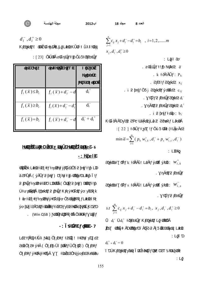
هنالك ثالث حاالت يمكن إن نقوم بهـا لتقليص المتغيرات
:[23 ] االنحرافية فـي دالة اإلنجـاز وكاآلتي
المتغيرات الصيغة العامة للقيد نوع القيد
االنحرافية
المراد تخفيضها
ii bxf ≤)( ii ddxf −+ −)(
di+
ii bxf ≥)( iii ddxf −+ +−)(
di-
ii bxf =)( ii ddxf −+ −)(
di- + di
+
استخدام برمجة األهداف لحل مسائل البرمجة - 6
-:الكسرية
أن دالة الهدف في مسائل البرمجة الكسرية يمكن تحويلها
واألخرى ) الهدف األول ( حدهما دالة البسط الى دالتين أ
طريقة برمجة األهداف أن وبما ) الهدف الثاني ( دالة المقام
تستطيع حل المشاكل ذات األهداف المتعددة والمتناقضة ،
لذلك يمكن استخدامها في حل مشاكل البرمجة الكسرية حيث
عند حل أعطت نتائج متطابقة مع الطريقة التكميلية المطورة
. Win QSB) ( باستخدام برنامج الجانب التطبيقي و
-: الجانب التطبيقي -7
مصنع البركة لصناعة الكراسي ينتج ثالثة أنواع من
وكل كرسي يمر ) رئاسي ، اعتيادي ، دراسي ( الكراسي
بأربعة مراحل هي مرحلة صب وسباكة هياكل الكراسي

م واثق حياوي اليذ.م القرارات ذات الدوال الكسرية باستخدام طريقة برمجة األهداف اتخاذ
156
10( ويتطلب , 20 المرحلة دقيقة على التوالي و ) 20 ,
الثانية هي مرحلة لحام وتشطيب هياكل الكراسي ويتطلب
)15, 20 دقيقة على التوالي والمرحلة الثالثة هي ) 30,
تصنيع المساند الجلدية والخشبية ويتطلب مرحلة
)10 , 20 دقيقة على التوالي والمرحلة الرابعة ) 40,
تطلب واألخيرة هي مرحلة التجميع والتغليف وت
)10 , 14 دقيقة على التوالي ، والزمن المتاح ) 30 ,
1500( هو للمراحل أسبوعيا ,2400, 1800 ,1500 (
كرسي الواحد هولل بيعالسعر فأذا كان ،دقيقة على التوالي
) 40 , 60 على التوالي وأن إلف دينار عراقي) 100,
32 ( الواحد هولكرسي الكلية ل كلفةال , 48 إلف ) 80,
أيجاد المزيج السلعي ، والمطلوب دينار عراقي على التوالي
.للمصنع األجمالي تعظيم دالة الربح األمثل الذي يؤدي إلى
-:الحل
-:نفرض أن
X .عدد الوحدات المنتجة من الكرسي الرئاسي = 1
X . من الكرسي االعتيادي عدد الوحدات المنتجة= 2
X .عدد الوحدات المنتجة من الكرسي الدراسي = 3
=)T ( مصنعاألجمالي لل ربحالدالة TT
c
r
-:حيث أن
T r =ةدالة اإليرادات الكلي .
T c = دالة التكاليف الكلية.
-:كون النموذج كاألتي في
XXXXXXTMax
321
321
3248804060100
++
++=
S.to
1500102020 321 ≤++ XXX
1800152030 321 ≤++ XXX
2400102040 321 ≤++ XXX
1500101430 321 ≤++ XXX
-: الحل بطريقة التكميلية المطورة 1‐
كون ت ما يمكن يجب إن كبر أدالة الربح الكلية تكون لكي
دالة الكلفة ما يمكن وكبرأ) البسط ( دالة اإليرادات الكلية
- : أن ما يمكن أيقلأ) المقام ( الكلية
XXXT rMax 321 4060100 ++=
XXXT cMin 321 324880 ++=
-:بالصورة اآلتية )المقام ( دالة الكلفة الكلية ويمكن كتابة
XXXT cMax 321 354880 −−−=
بالصورة ) الهدف الجديدة دالة ( الربح الكلية فتصبح دالة
-:اآلتية
TT cr MaxMaxTMax +=
XXXTMax 321 81220 ++=
باستخدام برنامج جانب التطبيقيتم كتابة وحل ال
Win QSB) ( في الشكل رقم )2( و ) 1.(

2012 اب 18 مجلد 8 العدد مجلة الهندسة
157
في جانب التطبيقييبين كتابة ال ) 1( الشكل رقم
التكميلية المطورة باستخدام الطريقة البرنامج
في جانب التطبيقياليبين حل ) 2( لشكل رقم ا
التكميلية المطورة باستخدام الطريقة البرنامج
- : طريقة برمجة األهداف - 2
باستخدام برنامج جانب التطبيقيتم كتابة وحل ال
)Win QSB ( في الشكل رقم )4( و ) 3.(
ي فجانب التطبيقييبين كتابة ال ) 3( الشكل رقم
البرنامج بطريقة برمجة األهداف
يبين حل المثال األول في ) 4( الشكل رقم
البرنامج بطريقة برمجة األهداف
وبالطريقتين نجد أنتطبيقيمن خالل نتائج الحل للجانب ال
- :المزيج السلعي هو
6,45,27 321 === XXX
T=5640(وأن أعظم إيرادات كانت r ( كلية كلفة وأقل
T=4512( كانت c( دالة الربح األجمالي قيمة ، أن
-:للمصنع هي
25.145125640
==T
أكبرمن دالة الربح األجمالي للمصنعقيمة بما أن
القرار المتخذ بأنتاج هذا أن فهذا يعني واحد
ي أرباحا ألدارة المصنع ، أما المزيج السلعي يعط
قل أ دالة الربح األجمالي للمصنعمة قيأذا كانت
القرار المتخذ بأنتاج هذا أن فهذا يعني من واحد
، أما خسائر ألدارة المصنعجلبالمزيج السلعي ي
تساوي دالة الربح األجمالي للمصنع أذا كانت
القرار المتخذ بأنتاج هذا أن فهذا يعني واحد
وال يجلب خسائر ي أرباحا يعطالمزيج السلعي ال
لمصنع الكلية ليرادات األ ، أي أن دارة المصنعأل
الكلية لألنتاج وعندها تسمى هذه كلفةالتساوي
. النقطة بنقطة التعادل
-: االستنتاجات – 8
توجيه اهتمام متخذي القرار في الشركات والمصانع - 1
اإلنتاجية إلى أهمية استخدام األساليب اإلدارية الحديثة
بحوث العمليات مثل نموذج واالعتماد على أساليب

م واثق حياوي اليذ.م القرارات ذات الدوال الكسرية باستخدام طريقة برمجة األهداف اتخاذ
158
بما يسهم في تحقيق أهداف هذه .البرمجة الكسرية
المنظمات، كما أنها توفر قدراً من المعلومات والبيانات
.التي تساعدها في القيام بوظائفها بفعالية وكفاءة عالية
تطابق نتائج الحل لنماذج البرمجة الكسرية باستخدام - 2
.ريقة برمجة األهدافالطريقة التكميلية المتطورة وط
أمكانية حل نماذج البرمجة الكسرية باستخدام برمجة - 3
األهداف وخاصة عندما تحتوي دالة الهدف على أكثر من
.كسر واحد
ساعد في ) Win QSB( استخدام البرنامج الجاهز - 4
.الجانب التطبيقي وبالطريقتينحل سرعة
References المصادر
مدخل كمي -الرقاية اإلدارية" مهدي حسين ، زويلف - 1
).1995( ، الطبعة األاولى،مكتبة الفالح، "
دراسة وتحليل طرائـق " ،وليد خالد جابر ، الحسناوي - 2
قسم ،رسالة ماجستير ، "حل مسائل البرمجة الكسرية
).2004(الجامعة التكنولوجية،العلوم التطبيقية
بحوث العمليات مفهوما "،حامد سعد نور ، ي الشمرت- 3
)2010(دار وائل للنشر، "وتطبيقا
احمد عبد ، الصفار،ماجدة عبد اللطيف محمد ، التميمي - 4
" بحوث العمليات تطبيقات على الحاسوب " ،اسماعيل
)2007.(دار المناهج للنشر والتوزيع عمان االردن
5‐ Bhatt S. K. ," Equivalence of various linearization algorithms for linear fractional programming",Volume 33, Number 1,p. 39-43 , (1989).
6- Crouzeix J.P. , Ferland J. A. و Schaible S. ," Duality in generalized linear fractional programming”, Mathematical Programming, Volume 27, Number 3 ،p.342-354 (1983).
7- Feng F., Xia Y. و Zhang Q. ," A Recurrent Neural Network for Linear Fractional Programming with Bound Constraints",(2006)
8- Arévalo M. T. , Mármol A. M. و Zapata A. ,” The tolerance approach in multiobjective linear fractional programming”, TOP, Volume 5, Number 2 ,p. 241-252, ( 1997 ).
9- Nemirovski A. ," The long-step method of analytic centers for fractional problems",Mathematical Programming,Volume 77, Number 1 ،p. 191-224,( 1997 ).
10- Mehra A. , Chandra S. و Bector C. R. ," Acceptable optimality in linear fractional programming with fuzzy coefficients",Fuzzy Optimization and Decision Making,Volume 6, Number 1,p. 5-16, (2007).
11- Nesterov Y. E. و Nemirovskii A. S. ," An interior-point method for generalized linear-fractional programming",Mathematical Programming,Volume 69, Numbers 1-3 ,p. 177-204, (1995).http://www.google.com, fractional linear programming
.12- Saleh M. " The Optimal Egyptian Cropping Pattern Using Nonlinear-Fractional Programming", Egyptian Informatics Journal, Vol. 6, No.1, June( 2005).
صياغة وحل نماذج البرمجة "،رشيد بشير ،رحيمه -13مجلة علوم " الكسرية باستخدام طريقة الآرانج المطورة
).2011 (5المجلد ، 7ذي قار العدد
حل مسائل البرمجة البرمجة "، رشيد بشير ، رحيمه -14لة علوم ذي مج" الهدفية الخطية باستخدام المصفوفات
) .2007 (1المجلد ، 1قار العدد
15- Katagiri H. و Sakawa M. ," A Study on Fuzzy Random Linear Programming Problems Based on Possibility and Necessity Measures",(2003).
16- Hamdy A.T.," operations research an introduction " seventh ed. Canada ,by Maxwell publishing company ,(2004) .

2012 اب 18 مجلد 8 العدد مجلة الهندسة
159
أستخدام طريقة تطوير مولد " حسن ،عباس أحمد ،-17قطع المستوي اليجاد الحل العددي لمسائل البرمجة
مجلة الهندسة والتكنولوجيا ، المجلد " الكسرية ).2008 ) (4( ، العدد 26
18- Rugg , M.M. , & White , G.P. & Endres ,
J.M. , (1983) “Using Goal Programming to
Improve Calculation of Diabetic Diels ” ,
Computer and Operation Research , Vol. 10
, P. 365-374 .
19- Martel J.M. and Aouni B., Incorporating the
Decision-Makers Preferences in the Goal-
Programming Model. [1990], Journal of the
Operational Research Society, Vol.(12):P ( 1121-
132 ).
20-Lin ,J.,Cheong , B. and Yao ,X. , Universal
multi-objective function for optimising
superplastic –damage constitutive equations ,[
2002 ] Journal of Materials processing Technolgy
Vol. ( 125 ) ,P( 199-205 ).
21-Leon , C. and Palacios F., Evaluation of rejected
cases in an acceptance system With data
envelopment analysis and goal programming , [
2009 ] Journal of the operational research Society
vol.( 60 ) ,P ( 1411-1420) .
22- Nesa , W. & Richard , C. (1981) , “ Linear
Programming and Extensions ” , McGraw – Hill ,
Inc.
23-Ignizio , J.P. , (1978) , “ A review of Goal
Programming : A Tool for Multiobjective
Analysis ” , J. op1.Res. Soc. , Vol. 29 , p. 1109-
1119 .
Journal of Engineering Volume 18 August 2012 Number 8
875
The Effect of Different Types of Aggregate and Additives on the Properties of Self-Compacting Lightweight Concrete
Qusay Jar-Allah Hachim By:
Assist. Prof. Dr. Nada M. Fawzi
Abstract The major aim of this research is study the effect of the type of lightweight aggregate (Porcelinite and Thermostone), type and ratio of the pozzolanic material(SF and HRM) and the use of different ratios of w/cm ratio(0.32 and 0.35) on the properties of SCLWC in the fresh and hardened state. SF and HRM are used in three percentage 5%,10%, and 15% as a partial replacement by weight of cement for all types of SCLWC. The requirements of self-compatibility for SCC are fulfilled by using the high performance superplasticizer (G51) at 1.2liter per 100 kg of cement. The values of air dry density and compressive strength at age of 28 days within the limits of structural lightweight concrete. The air dry density and compressive strength at age of 28 days for w/cm ratio(0.32) for SCLWC of Porcelinit aggregate are 1964 kg/m3 and 29.57 MPa, respectively. The corresponding values for the SCLWC of Thermostone aggregate are 1820 kg/m3 and 25.75 MPa, respectively. The results show that the HRM performance which is locally available is better than SF in production of SCLWC.
Keywords: Self-compacting lightweight concrete, porcelinite, thermostone, superplasticizer, silica fume, high reactivity metakaoline
المستخلصوزن ام الخفيف ال وع الرآ أثير ن يلينايت و الثرمستون ( إن الهدف الرئيسي من البحث هو دراسة ت ادة ) البورس سبة الم وع ون ون
ة وم (البوزوالني سليكا في ة وال اوؤلين عالي الفعالي ى االسمنت ) الميتاآ اء إل سبة الم ين من ن سبتين مختلفت 0.35 و 0.32(واستخدام ناؤولين . رسانة خفيفة الوزن ذاتية الرص في الحالة الطرية والحالة الصلبة على خواص الخ ) وم والميتاآ سليكا في استخدمت آل من ال
ة % 15،%10،%5عالي الفعالية بثالث نسب وزن ذاتي ة ال انة خفيف واع الخرس وع من أن آاستبدال جزئي من وزن االسمنت لكل ن .الرص
م 100لترلكل 1.2رص باستعمال الملدن عالي األداء بنسبة وقد تم تحقيق متطلبات الخرسانة ذاتية ال وع من آغ من االسمنت لكل نة الرص وزن ذاتي ة ال انة خفيف واع الخرس ر آانت . أن ضغاط بعم ة االن ة ومقاوم ة الجاف يم الكثاف انة 28ق وم ضمن حدود الخرس ي
ساوي يوم 28اإلنشائية خفيفة الوزن فالكثافة الجافة ومقاومة االنضغاط بعمر ى إسمنت ت اء إل ام 0.32 ولنسبة م انة ذات رآ لخرس ميكاباسكال على التوالي بينما آانت في الخرسانة ذات رآام 29.57 و 3م\ آغم 1964البورسيلينايت خفيف الوزن ذاتية الرص آانت
م 1820الثرمستون خفيف الوزن ذاتية الرص ائ 25.75 و 3م\ آغ د بينت النت والي وق ى الت اؤولين ميكاباسكال عل أن أداء الميتاآ ج ب .في إنتاج الخرسانة خفيفة الوزن ذاتية الرص) السليكا فيوم( عالي الفعالية المتوفر محليا أفضل من أداء المضاف

The Effect of Different Types of Aggregate and Additives on the Properties of Self-Compacting Lightweight Concrete
Qusay Jar-Allah Hachim
876
1-Introduction
Lightweight concrete (LWC) is a concrete which by one means or another has been made lighter than conventional concrete. Using concrete with a lower density can, therefore, result in significant benefits in terms of load-bearing elements of smaller cross-section and a corresponding reduction in the size of foundations. Furthermore, with lighter concrete , the formwork needs to withstand lower pressure than would be the case with normal weight concrete, and also the total mass of material to be handled is reduced with a consequent increase in productivity. Concrete which has a lower density also gives better thermal insulation than ordinary concrete and possesses good fire and frost resistance(Neville 2005). Self-compacting concrete (SCC) represents one of the most outstanding advances in concrete technology during the last decade. Due to its specific properties ,SCC can contribute significantly to the quality of concrete structures and open up new fields for the applications of concrete. SCC describes a concrete with the ability to compact itself only by means of its own weight without the requirement of vibration, it fills all recesses , reinforcement spaces and voids even in highly reinforced concrete members and flows free of segregation nearly to a level balance. Self-compacting lightweight concrete is a new building material which combines the known advantages of lightweight concrete and self-compacting concrete. Lightweight concrete with self-compacting ability offers considerable benefits, from reducing the density of concrete and providing self-compacting properties.
The workability of self-compacting lightweight concrete (SCLWC) can be characterized by the following properties (Badman 2003)
1. Filling ability: the ability of SCLWC to flow under its own weight (without vibration) to fill completely all spaces within intricate formwork, containing obstacles, such as reinforcement.
2. Passing ability: the ability of SCLWC to flow through openings approaching the size of the mix coarse aggregate. such as the spaces between steel, reinforcing bars, without segregation or aggregate blocking. This property is of concern in those application that involve placement in
complex shapes or sections with closely spaced reinforcement.
3. Segregation resistance (stability): the ability of SCLWC to remain homogenous during transportation , placing and after placement.
1-1 Development of Self-Compacting Concrete
For several years beginning in 1983, the problem of the durability of concrete structures was a major topic of interest. To make durable concrete structures, sufficient compaction by skilled workers is required. However, the gradual reduction in the number of skilled workers in construction industry has led to a similar reduction in the quality of construction work. One solution for the achievement of durable concrete structures, independent of the quality of construction work, is the use of self-compacting concrete, which can be compacted into every corner of a formwork, purely by means of its own weight and without the need for vibrating compaction (Ouchi 1999).
1-2 The methods for achievement self-compatibility
Okamura and ouchi (2003) have employed the following methods to achieve self-compatibility:
1-limited aggregate content;
2- low water-powder ratio;
3- Use of superplastizer.
They found also that the highly viscous paste is also required to avoid the blockage of coarse aggregate when concrete flows through obstacles, High deformability can be achieved by the employment of a super plasticizer, keeping the water-powder ratio to a very low value. They have also found that the frequency of collision and contact between aggregate particles can increase as the relative distance between the particles decreases and then internal stress can increase when concrete is deformed, particularly near obstacles. They have concluded that the energy required for flowing is consumed by the increased internal stress, resulting in blockage of aggregate particles. Limiting the coarse aggregate content to a level lower than normal, which is effective in avoiding this kind of blockage.

Journal of Engineering Volume 18 August 2012 Number 8
877
1-3Structural lightweight concrete (SLWC)
The (American Concrete Institute) (ACI 213R-91) defines the structural lightweight concrete as a concrete which (a): has a minimum compressive strength at 28 days of 17.2MPa,(b): has a corresponding air-dry unit weight in a range of 1440 to 1850 kg/m3 and (c): consists of all lightweight aggregate LWA or a combination of LWA and normal weight aggregates.
Al-Rawi(1995) has studied the properties of Porcelinite lightweight aggregate to produce LWC. 18 mixes in various mix proportion are prepared without using any admixture. Cement content was between 272 - 687kg/m3 and water/cement ratios ranged between 0.65-1.6.The lightweight concrete used in this investigation can offer a compressive strength up to 32MPa with an air dry density of 1815 kg/m3 at 28 days.
1-4 Self-Compacting Lightweight Concrete
(SCLWC)
Self-compacting lightweight concrete (SCLWC) is a new high-performance building material, which combines the well-known advantages of lightweight concrete with those of self-compacting concrete (SCC).
Kobayashi (2001) has examined the characteristics of SCC in fresh state with artificial lightweight aggregate (LWA).Whereas, the artificial LWA has lower water absorption ratio than ordinary LWA because of its tight surface structure, and can be used for concrete mixing without pre-wetting procedure. Another advantage of this aggregate is its spherical shape that is expected to increase fluidity of concrete. The results show that SCC with this aggregate has higher self-compactability than that with crushed stone, while the deformation rate of concrete is very small. Segregation between the aggregate and mortar, however, tends to be large because of larger difference of specific gravity between them than in the case of ordinary self-compacting concrete with crushed stone. Increase in unit mass of the lightweight aggregate does not affect so much on self-compactability of concrete.
2- Objective of the research
The main objective of this study is to investigate the effect of the following variables on the properties of SCLWC in the fresh and hardened states:
1. type of lightweight aggregate by using porcelinite and waste crushed Thermostone aggregate.
2. type of mineral admixtures by using silica fume (SF) and high reactivity metakaoline (HRM).
3. Water cement ratio by using two values of 0.32 and 0.35.
Results of this research will provide information about the rheological and mechanical properties of self-compacting lightweight concrete. High performance superplasticizer (Glinume 51) is used as chemical admixture in this study. In this study, the self-compatibility tests (Slump flow, V-Funnel, L-Box, U-Box) were performed on the fresh concrete for each mix of SCLWC. Air dry density at 28 days, compressive strength and splitting tensile strength at 7,28,90 day tests are conducted. 28 concrete mixes are investigated in fresh and hardened state. A total of 252 concrete cubes of 150 mm, 252 concrete cylinders of 150×300 mm, are cast, cured and tested for this study.
3- Experimental work
3-1 Materials Cement
AL-Shemalia ordinary Portland cement manufactured in Kingdom of Saudi Arabi (KSA) is used in this research. the results of the chemical analysis and physical properties of the cement indicate that the available cement is conformed to the Iraqi Specification as shown in Table 1and Table2 ( Chemical and Physical properties of cement are performed by the State Company of Geological Survey and Mining.)
Water potable water is used as a mixing water for all concrete mixes.
Sand Al-Ekhaider sand of 4.75 mm maximum size is used as fine aggregate in concrete mixes

The Effect of Different Types of Aggregate and Additives on the Properties of Self-Compacting Lightweight Concrete
Qusay Jar-Allah Hachim
878
the results of the chemical analysis and physical properties of the sand indicate that the available sand is conformed to the Iraqi Specification as shown in Table 3.( Chemical and Physical properties of sand are performed by the State Company of Geological Survey and Mining.)
Coarse aggregate • Porcelinite Aggregate
Crushed stone Porcelinite has been used as coarse aggregate in this study with max. size 9.5 mm
• Thermostone Aggregate Thermostone aggregate is considered as one of the industrial residual which is accumulated during industrial process of Thermoston blocks. it used with max. size 9.5 mm. The grading and physical properties of Porcelinite and Thermos tone aggregate conform to the requirements of the ASTM C330 as shown in Fig. 2 and Table 4 respectively. (Physical properties of Porcelinite and Thermestone are performed by the State Company of Geological Survey and Mining) . Table (4a) indicate the sieve analysis of coarse aggregate.
Chemical Admixture A high performance concrete superplasticizer Glinume 51 (G51) is used in this research as chemical admixture .G51 complies with ASTM C494 Types A and F
Mineral admixture: • Silica fume (SF)
The chemical analysis of SF was used in this research conforms to the chemical requirements of ASTM C1240 as shown in Table5 and Table 6.
• High Reactivity Metakaoline(HRM) The chemical analysis of HRM was used in this research conforms to the chemical requirements of ASTM C618 respectively as shown in Table 7 and Table 8. (Chemical analysis of HRM and SF are performed by the State Company of Geological Survey and Mining ) 3-2 Design of Concrete Mixes
The design of SCLWC mixes is performed to produce structural lightweight concrete conforms to the requirements of structural LWC, according to ACI Committee 213 In the same time, the mix deign of SCLWC must satisfy the criteria of filling ability, passing ability and segregation resistance. The mix design method of SCC used in the present study is according to EFNARC 2005, Two series are used throughout this research, Porcilinite aggregate is used as a
coarse aggregate in the first series, Thermostone aggregate is used as a coarse aggregate in the second series. Two w/c ratios (0.32 and 0.35) are adjusted for each mix and The optimum dosage of GLINUME51(G51) (1.2 liter per 100 kg of cement) For all mixes, cement content is 500 kg/m3 , fine aggregate is 590 kg/m3 and coarse aggregate is 620 kg/m3. The optimum dosage of GLINUME51(G51) (1.2 liter per 100 kg of cement) is obtained from several trail mixes incorporating G51,by increasing the dosage of the admixture gradually ,and fixed the w/cm ratios (0.32and 0.35) to ensure the self-compactability as shown in Fig.1.
3-3 Mixing of concrete
The Porcelinite and Therrmostone aggregate is used in saturated surface dry (SSD) ,which is recommended by the ACI committee 211-2 . In this study the method of Emborg2000 is used in the mixing of reference concrete (LWC) and self-compacting lightweight concrete. This method includes the following steps for reference concrete:
1.The dry quantity of fine aggregate is mixed with 1/3 of mixing water for 1 minute.
2.The quantity of cement with 1/3 of mixing water is added to the mix and the mixture is mixed for about 1 minute.
3.The quantity of coarse aggregate plus 1/3 of mixing water+1/3 of the dosage of the admixture are added to the mix and the mixture is mixed for about 1 minute after that leave the mixture to rest for 1.5 minute.
4. The remained dosage of the admixture is added to the mix and the mixture is mixed for about 1.5 minute.
For mixing the SCLWC the same steps as shown above except before adding the quantity required of cement, the required quantity of mineral admixture (S.F or HRM) is added by the weight of cement and mixed with the cement only for about 15 second to disperse all the particles of mineral admixture(S.F or HRM) throughout the cement grains.

Journal of Engineering Volume 18 August 2012 Number 8
879
3-4 Testing of concrete
Testing of Fresh Concrete
• Slump test was used to determine the workability for reference concrete. This test is performed according to ASTM C143.
• Slump Flow Test, V-Funnel test, L-Box Test and U-Box Test were used to characterize the properties of SCLWC (filling ability, passing ability and segregation resistance these tests were performed according to EFNARC 2002 and EFNARC 2005 .
Testing of Hardened Concrete
• Compressive Strength: The compressive strength test is carried out on 150mm cubes This test was performed according to BS1881:part 116 The specimens are tested at ages of 7,28 and 90 days and in each age the average of three specimens are adopted.
• Splitting Tensile Strength: The splitting tensile strength test is performed according to ASTM C496 ,150×300 mm cylindrical concrete specimens are used. The specimens are tested at age of 7,28 and 90 days and in each age the average of three specimens has been adopted
• Hardened Unit Weight (28 Days Air Dry Density): This test is used to determine the air dry density of concrete mixes Cubes specimens of 150mm are used in this test at age of 28 days the test is performed according to ASTM C567.
4- Properties of Fresh SCLWC
• Slump Flow: The results of Slump flow test ranged between 657- 712 mm for SCLWC mixes produced from Porcelinite aggregate and range between 679--769 mm for SCLWC mixes produced from Thermostone aggregate. These results are within the acceptable criteria for SCC
and indicate also excellent deformability and filling ability without any segregation ,bleeding and blocking.
V-Funnel: The values of flow time (TV) range between 9.8-12.4 sec and 6.4-11.5 sec for SCLWC mixes produced from Porcelinite
aggregate for w/cm ratio 0.32 and 0.35 respectively. The values of flow time (TV5) range between 10.6-15.2 sec and 8.5-14.5 sec for SCLWC mixes produced from Porcelinite aggregate for w/cm ratio 0.32 and 0.35 respectively.. Values of flow time (TV) range between 6.5-11.5 sec and 6-10.5 sec for SCLWC mixes produced from Thermostone aggregate for w/cm ratio 0.32 and 0.35 respectively. Values of flow time (TV5) range between 7.8-13.7 sec and 7.4-12.8 sec for SCLWC mixes produced from Thermostone aggregate for w/cm ratio 0.32 and 0.35 respectively. These results are within the acceptable criteria for SCC(EFNARK 2002).
L-Box: The results of L-Box test blocking ratio (H2/H1) range between 0.8-0.94 for all mixes of SCLWC. These results are within the acceptable criteria for SCC and indicate that the mixes have excellent passing ability.
• U-Box: The results of U-Box test filling height (H1–H2) range between 12-28 mm for all mixes of SCLWC. These results are within the acceptable criteria for SCC.
5- Hardened Concrete Properties
• Compressive Strength: The results of compressive strength test for all concrete mix in this study at 28 days are higher than 17 MPa, the minimum required strength recommended by ACI-213 for structural LWC. At early ages (7 days) (see Fig3) for the same w/cm ratio the compressive strength for all concrete mix of SCLWC containing SF is higher than concrete mix of SCLWC containing HRM and reference mix The contribution of silica fume to the early strength development (up to 7 days) is through improvement in packing and the interface zone with aggregate (Neville 2002) While for HRM, the dilution effect of it, when is used as a partial replacement for cement. The concrete mixture will also experience some effect of the removal of cement from reacting system and that affecting the early compressive strength (Justice 2005) For this reason, all concrete mixes of SCLWC containing HRM give compressive strength at 7days less than the compressive strength of reference concrete at the same age. At 28 and 90 days (see Figs. 3) for the same w/cm ratio the compressive strength for all concrete mixes of SCLWC containing HRM was higher than concrete mix of SCLWC containing SF.
The Effect of Different Types of Aggregate and Additives on the Properties of Self-Compacting Lightweight Concrete
Qusay Jar-Allah Hachim
880
This is due to high pozzolanic activity of HRM if compared with SF(P.A.I for SF=108%, for HRM=140%) as HRM the major components responsible for the pozzolanic reaction are alumina and silica (Advanced Cement Technology 2002) From the chemical composition of HRM used in this study, the sum percentage of alumina(AL203) and silica(SIO2) is 91.17%, more than the percentage of amorphous silica (SIO2) in SF which is responsible for the pozzolanic reaction(ACI234R-96) (SIO2=87.45% for SF used in this study). The pozzolanic reaction take place between the components mentioned above in pozzolanic material (SF and HRM) and calcium hydroxide CH formed during the hydration process. This leads to the cementations compound which is produced from the reaction of HRM more than the cementations compound which is produced from the reaction of SF and this leads to densification of the concrete matrix resulting in a considerable increase in strength ,and reduction in permeability. Besides, the pore-size and grain-size refinement processes associated with pozzolanic reaction can effectively reduce the microcraking and strengthen the transition zone (Mehta et al 2006).
• Splitting Tensile Strength: Due to the usage of mineral admixtures(SF and HRM), chemical admixtures (Glinume 51) , in addition to the self- compactability, an improvement to the ITZ is expected. Consequently, good results of tensile strength are expected. Figs(4) show that at early ages (7 days) and for the same w/cm ratio splitting tensile strength of SCLWC mixes containing SF is higher than SCLWC mixes containing HRM and reference mixes. This is due to the physical effect of silica fume and the ability of the extremely fine particles of silica fume to be located in very close proximity to the aggregate particles, that is, at the aggregate-cement paste interface, and this allows to the cement particles packing tightly against the surface of the aggregate, and this leads to strengthen the ITZ. A contributing factor is the fact that silica fume because of its high fineness, reduces bleeding so that no bleed water is trapped beneath coarse aggregate particles. Consequently, the porosity in the ITZ is reduced then splitting tensile strength increased (Neville 2002) . Due to the dilution effect of HRM when it is used as a partial replacement of cement, splitting tensile strength at 7 days of SCLWC mixes containing HRM is less than reference mixes (LWC) . At
28,90 days and for the same w/cm ratio Figs(4) show that the splitting tensile strength of SCLWC mixes containing HRM is more than SCLWC mixes containing SF, this because of high pozzolanic activity of HRM if compared with SF as shown in pervious section. The pozzolanic reaction strengthen the transition zone through processes of pore size and grain size refinement ,thus reducing the microcracking of concrete. in addition the well and uniform dispersion of cement and particles of mineral admixture (HRM and SF) by the action of superplasticizer (Glinume 51) leads to a great improvement in tensile strength (Mehta et al 2006)(Druta 2003).
• Hardened Unit Weight (28 day air dry density): The results show that the 28 days air dry density for concrete mixes produced from Thermostone aggregate conform to the requirement of ACI 213 for structural LWC. The 28 days air dry densities for concrete mixes produced from Porcelinite aggregate more than 1850 kg/m3 ,but they are below 2000 kg/m3 . However all concrete mixes in this study conform to the requirement of structural lightweight aggregate concrete, according to British specification which limits the maximum density of structural lightweight concrete to 2000 kg/m3. The 28 days air dry densities for SCLWC mixes containing HRM more than SCLWC mixes containing SF(see Fig. (5)). This is due to the highly pozzolanic activity of HRM if compared with SF. The Cementation compound that results from the pozzolanic reaction of HRM is more than the cementation compound that result from pozzolanic reaction of SF, and this leads to an increase in cement gel and density. From Fig.(5). The results show that the 28 days air dry densities of all SCLWC mixes are more than reference concrete mixes (LWC), this behavior can be ascribed to the pozzolanic reaction of mineral admixture(HRM and SF) in SCLWC mixes. The pozzolanic reaction leads to an increase in cement gel (the cementation compounds), it also leads to the densification of concrete matrix and the transition zone through the processes of pore-size and grain-size refinement(Mehta et al 2006). 6- Conclusions
1. It is possible to produce SCLWC by using two types of locally available porcelinite or thermostone as coarse lightweight aggregate, high performance superplasticizer (Glinume51)

Journal of Engineering Volume 18 August 2012 Number 8
881
and highly active pozzolanice materials (HRM and SF).
2. Results of this investigation indicated that locally available HRM performs better than SF in produced SCLWC.
3. The SCLWC mixes produced from Porcelinite aggregate showed considerable improvement in all mechanical properties compared with SCLWC mixes produced from Thermostone aggregate.
4. at 28 days There is a positive relationship between the air dry density and compressive strength and the percentage of the added pozzolanic material and the compressive strength of the SCLWC mixes.
5. There is no significant increase in all mechanical properties of SCLWC mixes for w/cm ratio 0.32 if compared with SCLWC mixes for w/cm ratio 0.35.
6. There is no significant increase in all mechanical properties of SCLWC mixes for w/cm ratio 0.32 if compared with SCLWC mixes for w/cm ratio 0.35.
7. The values of air dry density and compressive strength for SCLWC mixes produced from Thermostone aggregate at 28 days are within the requirements limits of structural LWC. At 28 days, the air dry density ranges between 1710-1820 kg/m3 and 1688 -1795 kg/m3 for w/cm ratio 0.32 and 0.35 respectively. The compressive strength ranges between 20.14 -25.75 MPa and 19.89 -25.21 MPa w/cm ratio 0.32 and 0.35 respectively. For reference concrete (LWC) the 28 days air dry density falls between 1683 and1653 kg/m3 and the compressive strength falls between 18.50 and 17.88 MPa for w/cm ratio 0.32 and 0.35 respectively. the splitting tensile strength at 28 days ranges between 2.55 -3.09 MPa and 2.35 -2.89 MPa for w/cm ratio 0.32 and 0.35 respectively. For reference concrete (LWC), the splitting tensile strength at 28 days falls between 2.44 and 2.19 MPa for w/cm ratio 0.32 and 0.35 respectively.
8. The values of air dry density and compressive strength for SCLWC mixes produced from Porcelinite aggregate at 28 days are within the requirements limits of structural LWC. At 28 days, the air dry density ranges between 1907-1964 kg/m3 and 1844-1944kg/m3 for w/cm ratio 0.32 and 0.35 respectively. The compressive strength ranges between 24.12 -29.57 MPa and 22.22 -27.89 MPa w/cm ratio 0.32 and 0.35 respectively. For reference concrete (LWC) the 28 days air dry density falls between 1890 and 1823 kg/m3, and compressive strength falls between 21.76 and 20.5 MPa for w/cm ratio 0.32 and 0.35 respectively. The splitting tensile
strength at 28 days ranges between 3.17 -3.77MPa and 2.84 -3.27 MPa for w/cm ratio 0.32 and 0.35 respectively. For reference concrete (LWC), the splitting tensile strength at 28 days falls between 2.91 and 2.69 for w/cm ratio 0.32 and 0.35 respectively.
References
• Qusay, J.H " The effect of different types of aggregate and additives on the properties of Self-Compacting Lightweight Concrete" M.SC. Thesis, Baghdad University, February 2011.
• ACI Committee 213, "Gide for Structural Lightweight Aggregate Concrete", ACI 213R-87, ACI Manual of concrete practice, Part 1, 1991, pp.213R-1-27.
• ACI Committee 211, "Standard Practice for Selecting Proportion for Structural Lightweight Concrete", ACI 211.2-98, ACI Manual of concrete Practice, Part1, 1998, pp.211.2-98
• ACI Committee 234, "Gide for the Use of Silica Fume in Concrete", ACI 234R-96, ACI Manual of concrete practice, Part 1, 1996, pp.234R-1-41.
• Advanced Cement Technology, LIC, "High Reactivity metakaolin engineered material admixture for use with Portland cement", 2002, pp.7, www.metakaolin.com, Email: sales@ metakaolin.com.
• ASTM C330-03," Standard Specification for Lightweight Aggregates for Structural Concrete", Annual Book of ASTM Standards,2003.
• ASTM C 494/C 494M – 05a, " Standard Specification for Chemical Admixtures for Concrete", Annual Book of ASTM Standards,2005.
• ASTM C 1240-03 " Standard Specification for Use of Silica Fume as a Mineral Admixture in Hydraulic-Cement Concrete, Mortar, and Grout ", Annual Book of ASTM Standards,2003
• ASTM C 618 – 03" Standard Specification for Coal Fly Ash and Raw or Calcined Natural Pozzolan for Use in Concrete", Annual Book of ASTM Standards,2003.
• ASTM C 143/C 143M – 05a" Standard Specification for Slump of Hydraulic-Cement Concrete", Annual Book of ASTM Standards,2005
• ASTM C 496/C 496M – 04" Standard Test Method for Splitting Tensile Strength of Cylindrical Concrete Specimens", Annual Book of ASTM Standards,2004.

The Effect of Different Types of Aggregate and Additives on the Properties of Self-Compacting Lightweight Concrete
Qusay Jar-Allah Hachim
882
• ASTM C 567-05A " Standard Test Method for Determining Density of Structural Lightweight Concrete", Annual Book of ASTM Standards,2005
• Badman, C., '' Interim Guidelines for the use of Self- Consolidating Concrete in PCI Member Plant '', PCI Journal, Vol.48, No.3, May/June 2003, pp.14-18
• BS1881, Part1, 1985, " Code of Practice for Design and Construction ", British Standards Institution
• BS 1881, Part 116, 1989, " Method for Determination of Compressive Strength of Concrete Cubes", British standards institution
• Druta, C., " Tensile Strength and Bonding Characteristics of Self-Compacting Concrete", M.SC. Thesis, Louisiana state university, August 2003, pp .125.
• EFNARC, "Specification and Guidelines for Self-Compacting Concrete", Feruary 2002, pp.32, www.efranice.org
• Justice, J.M., "Evaluation of Metakaolin for Use as Supplementary Cementitious Materials", M.Sc. Thesis, Georgia institute of Technology, April 2005, pp. 134
• M., Emborg, " Mixing and transport ", Final Report, Task 8.1, University of Paisly, June 2000, pp.65
• Mehta,P.K., and Monterio P.J, "Concrete: Microstructures, Properties and Materials", McGraw-Hill, United States of America, Third Edition, 2006, pp.684.
• Neville, A.M., "Properties of Concrete", Longman Group, Ltd., 4th and Final Edition, 2000, pp. 844
• Shindoh, T., and Matsuoka, Y., "Development of Combination- Type Self-Compacting Concrete
and Evaluation Test Methods" Journal of Advanced Concrete Technology, V.1, No.1, April 2003, pp.26-36
• Okamura, H., and Ouchi, M., '' Self-Compacting Concrete'', Journal of Advanced Concrete Technology, Vol. 1, No.1, April 2003, pp.5-15.Ouchi, M. "Self-Compacting Concrete: Development, Applications and Investigations'', Nordic Concrete Research, 1999, pp.29-34
• The Self-Compacting Concrete European Project Group, "The European Guidelines for Self-Compacting Concrete", may 2005, pp.63
ز، • د العزي رقي عب صي ش راوي ق واص الخر"ال ة خ انة خفيف سي لينايت المحل ام البورس ن رآ صنعة م وزن الم ة "ال ، اطروح
1995ماجستير ، جامعة بغداد ، م • ة رق ية ألعراقي فة ألقياس سنة ) 5(ألمواص منت "1985ل أألس
دي ة ، "ألبورتالن سيطرة النوعي يس أل زي للتقي از المرآ . الجه
رآام ألمصادر "1984لسنة ) 45(سية ألعراقية رقم ألمواصفة ألقيا •اء از المرآزي ، "الطبيعية ألمستعملة في ألخرسانة والبن الجه
.للتقييس والسيطرة النوعية
List of Abbreviations
Calcium HydroxideCH
Calcium Silicate Hydrate C-S-H
Glinume 51G51 High Reactivity Metakaoline HRM Interfacial Transition ZoneITZ Lightweight AggregateLWA Lightweight ConcreteLWC Pozzolanic Activity IndexPAI Reference Ref.
Self-Compacting ConcreteSCC Self-Compacting Lightweight Concrete SCLWC

Journal of Engineering Volume 18 August 2012 Number 8
883
Saturated Surface Dry SSD
Silica FumeSF Water to Cementitous Material Ratio w/cm
Flow time of V- funnel test after 5 minutes TV5
Table (1) Chemical composition and main compounds of cement
Oxide composition
% by weight Limits of Iraqi Specification no.5 / 1984
SIO2 19.59 Not available
Fe2O3 3.53 Not available
AL2O3 4.63 Not available
Cao 61.58 Not available
Mgo 2.75 5.0(max)
SO3 2.74 2.8(max)
Loss on ignition 1.64 4.0(max)
Insoluble residue 0.78 1.5(max)
Lime saturation factor 0.95 0.66-1.02
Main compounds ( Bogue’s equation )% by weight of cement
C3S 57.78 Not available
C2S 12.89 Not available

The Effect of Different Types of Aggregate and Additives on the Properties of Self-Compacting Lightweight Concrete
Qusay Jar-Allah Hachim
884
Table (2) Physical properties of cement
Physical property Test result Limits of Iraqi Specification no.5/1984
Specific surface area (blaine method), m²/kg
240 230 (min)
Setting time (vicate’s method)
Initial setting, hrs:min
Final setting, hrs:min
1:00
6:00
00:45 (min)
10:00 (max)
Compressive strength, mpa
3 days
7 days
17.6
26.8
15.00 (min)
23.00 (min)
Autoclave expansion, % 0.5 0.8 (max)
Table (3) Chemical and physical properties of sand
Property Test result Limit of Iraqi Specification no .45/1984
Specific gravity. 2.54 Not available
Absorption, % 2.97 Not available
Dry loose unit weight, kg/m³ 1587 Not available
Sulphate content as so3,% 0.07 0.5(max)
Material finer than 75µm, % 2.6 5.0(max)
Table(4) Physical properties of the Porcelinite and Thermostone aggregate
Thermostone Porcelinite Aggregate
1.14 1.52 Sspecific gravity
53.6 32.85 Absorption, %
560* 765* Bulk density(dry loose), kg/m³
*within the limits of ASTM C330 (880 kg/m³ max. ) for coarse aggregate.
C3A 6.31 More than 5%
C4AF 10.73 Not available

Journal of Engineering Volume 18 August 2012 Number 8
885
Table (4a) Sieve analysis of coarse aggregate(Porcelinite and Thermestone)
Cumulative passing%(Limits of
ASTM C330)
Cumulative passing % Sieve size (mm)
100 100 12.5
100-80 95 9.5
5-40 30 4.75
20-0 11 2.36
10-0 0 1.18
Table (5) Chemical analysis of SF
Oxide content % Oxide composition
87.45 SIO2
0.35 AL2O3
1.17 Fe2O3
2.4 Mgo
1.25 Cao
0.91 SO3
3.78 L.O.I
1.37 Na2O
Chemical requirements of SF according to ASTM C I240 Table (6)
Limits of ASTM C1240 S.F. Oxide composition
85.0 87.45 SiO2,min.,%
6.0 3.78 Loss on ignition, max %

The Effect of Different Types of Aggregate and Additives on the Properties of Self-Compacting Lightweight Concrete
Qusay Jar-Allah Hachim
886
Table (7) Chemical analysis of HRM
Table (8) Chemical requirements of HRM according to ASTM C 618
Fig. (1) Illustrative figure of self-compactability(Shindoh et al 2003)
Oxide content %Oxide composition
54.88SiO2
36.29AL2O3
1.4Fe2O3
0.21Mgo
0.38CaO
0.21SO3
2.47L.O.I
0.66Na2O
Oxide composition HRM Pozzolan class N
SiO2 + AL2O3 + Fe2O3, min. % 92.57 70
SO3, max. % 0.21 4
Loss on ignition max 2.47 10
Journal of Engineering Volume 18 August 2012 Number 8
887
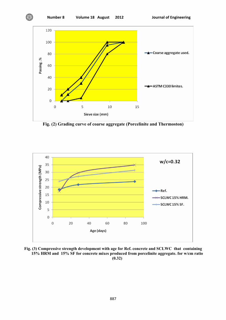
Fig. (2) Grading curve of coarse aggregate (Porcelinite and Thermoston)
Fig. (3) Compressive strength development with age for Ref. concrete and SCLWC that containing 15% HRM and 15% SF for concrete mixes produced from porcelinite aggregate. for w/cm ratio
(0.32)

The Effect of Different Types of Aggregate and Additives on the Properties of Self-Compacting Lightweight Concrete
Qusay Jar-Allah Hachim
888
Fig. (4) Splitting tensile strength development with age for Ref. concrete and SCLWC that containing 15% HRM and 15% SF for concrete mixes produced from porcelinite aggregate
for w/cm ratio (0.32)
Fig. (5) 28 days air dry density for all concrete mixes for w/cm ratio (0.32)

Journal of Engineering Volume 18 August 2012 Number 8
889
Effect of Fire Flame (High Temperature) on the Behaviour of
Axially loaded Reinforced SCC Short Columns Amer F. Izzat
University of Baghdad Lecturer in Civil Engineering Depart.
Abstract: Experimental research was carried out to investigate the effect of fire flame (high temperature) on specimens of short columns manufactured using SCC (Self compacted concrete). To simulate the real practical fire disasters, the specimens were exposed to high temperature flame, using furnace manufactured for this purpose. The column specimens were cooled in two ways. In the first the specimens were left in the air and suddenly cooled using water, after that the specimens were loaded to study the effect of degree of temperature, steel reinforcement ratio and cooling rate, on the load carrying capacity of the reinforced concrete column specimens. The results will be compared with behaviour of columns without burning (control specimens). The results showed that, the ultimate load capacity of columns exposed to fire decreases with increasing the fire flame temperature. At burning temperature 300 Co , 500 Co and 700 Co , the average residual ultimate load capacity for gradually cooled specimens were 91%, 81% and 71% respectively. By increasing the ratio of longitudinal reinforcement 44% , the maximum improvement in the ultimate load capacity was 24% and 17% for the gradually and sudden cooling respectively at Co500 . For the same longitudinal reinforcement ratio and fire burning temperature, the ultimate capacity for the sudden cooling specimens was less than that of gradually cooled specimens by about 10%.
Key word: self compacted concrete (SCC), elevated temperature, fire flame.
:الخالصةة رارة العالي ات الح اثير درج ة ت ي اجرى لدراس ق(بحث عمل صيرة ،) الحري انية الق دة الخرس ن االعم اذج م ى نم عل
ة الرص ة . المسلحة والمصنعة باستخدام الخرسانة الذاتي درجات حرارة عالي ى لهب ب اذج عرضت ال باستخدام ، النم .فرن صنع لهذا الغرض
اذج بطريقتين الحريق الحقيقية آارثة لمحاآات د النم اء ، في الموقع تم تبري د فجائي باستخدام الم د بطيء وتبري . تبري : تاثيرومن ثم يتم تحميلها لدراسة
.)تدريجي و فجائي(ومعدل التبريد ، الحرق نسب حديد مختلفة بعد ، تاثير لهب الحريق في درجات حرارة مختلفة ).االعمدة التي لم تتعرض للحريق( قارنة النتائج مع نماذج السيطرةعلى قوة تحمل االعمدة الخرسانية المسلحة وم
و % 81، %71حيث وصلت الى ، ان مقاومة تحمل العمود لالحمال تقل آلما زادت درجة الحرارة، هرت النتائج ظا % 44بزيادة نسبة حديد التسليح الطولي بمقدار . Co700 و Co300،Co500للنماذج المعرضة الى % 91
للنموذج المبرد تدريجيا وفجائيا بالتتابع عند درجة حرارة % 17و % 24آانت اعلى زيادة في قوة تحمل العمود Co500..
ة المبردة فجائيا اقل تحمال من الحديد الطولي ولنفس درجة الحرارة فان االعمدوجد انه عند استخدام نسبة مماثلة %.10مال من المبردة تديجيا بمقدار حلال

Effect of Fire Flame (High Temperature) on the Behaviour of Axially loaded Reinforced SCC Short Columns
Amer F. Izzat
[
890
Introduction: Many researchers studied the
effect of fire on concrete, reinforcement, bond strength between them and the behavior of different reinforced concrete members. Most of tests were done using electrical furnaces to expose such members to elevated temperature, where only heat is supplied, while in real fire, the members are subjected to the flame which accompanied with different gasses. Another problem must be simulated which is the sudden cooling of the reinforced concrete members due to the way of controlling the fire by using water. Most of the researchers a greed that the damages in the concrete mix started at temperature above 300 Co , because the porosity of cement paste increased rapidly to formation of micro cracks [Piasta et al 1984] due to dehydration of some cement paste compounds. Beyond 500 Co additional increase in porosity caused by liberation of water from the dissociation of Ca(OH)2 in the range 450-550 Co and liberation of CO2 as a result of CaCO3 decomposition above 600 Co [Piasta et al 1984]. For reinforced concrete members, [Robston T.D. 1962] found that till 100 Co the thermal expansion in the steel reinforcement is approximately similar to that of the normal concrete, above this temperature the expansion of the steel will increase while the concrete will suffering from shrinkage due to the dehydrate of cement, this will cause loosens in the bond between concrete and steel reinforcement and cracks will started to form and grow. [Harada et al 1972] they found that the residual bond strength between the concrete and the reinforcement was 44% of the control specimens at a temperature of 300 Co and dropped rapidly to 10% at 450 Co , while the residual strength of compressive strength was 60% at the similar temperature.
Material Properties: - The cement used in this study was Ordinary Portland Cement complying with ASTM C150-02. Test results are shown in Tables 1 and 2 for the chemical and physical properties respectively. - The coarse aggregate used was natural aggregate with 10mm maximum size of aggregate. The grading obtained from the results of sieve analysis of the aggregate lies within the range defined by ASTM C33-03. - The results of sieve analysis which was carried out on fine aggregate lies also within the range defined by ASTM C33-03. The chemical and physical test results for gravel and sand are shown in Tables 3 and 4 respectively. - Glenium 51: (modified polycarboxylic ether) was used as a water reducing agent plus stabilizing agent with a specific gravity of 1.1, at 20oC, PH = 6.5 as issued by the producer. - Silica fume mineral admixture or micro silica: composed of ultrafine, amorphous glassy spheres of silicon dioxide (SiO2), produced by Crosfield Chemicals, Warrington, England.
Concrete mix proportions: Several trail mixes were used.
The final mix proportions used is 1:1.5:1.6 with water cement ratio 0.5 in addition to 3 liters of glenium-51 admixture for each 100kg of cement was used. The mixture proportions are summarized in Table 5 .
The slump flow for the self compacted concrete was 685mm (using cone test-ASTM C1611-05 ) and the slump test for the normal concrete was 100mm (ASTM C143-00 ).
Deformed steel bars of diameter 10mm and 12mm were used as longitudinal reinforcement. While for the ties reinforcement 3mm smooth bar diameter was used. Determine their tensile properties according to ASTM

Journal of Engineering Volume 18 August 2012 Number 8
891
615-05a. The results are shown in Table 6.
The mixing of concrete was carried out in a tilting pan type mixer of 0.1m3 capacity. In all the mixes, the aggregates and cement were first mixed dry for about 90seconds. The water, silica fume and the superplasticizer together were mixed externally in a pan then added to the pan mixer, after that mixing continued, for a further 90seconds. With each beam six (100mm x 100 mm x 100mm) cubes were cast to determine the compressive strength of the hardened concrete.
Experimental Program: Twelve reinforced concrete
columns were tested, with overall length of 700mm and cross-sectional area of 100 x 100mm as shown in Fig. 1-A. All columns specimens have a top and bottom bearing hat with a square tied ring all made of 2mm thick steel plate to prevent end bearing failure of the two ends and to be insure that the load are distributed uniformly overall the column ends. Specimens were tested in the structural lab of Al-Mustanseria University. All specimens were reinforced with four longitudinal steel bars, as shown in Table 7. Specimens C1 to C6 were reinforced with 4 - 10φ mm, while C7 to C12 were reinforced with 4 -
12φ mm. Ties were made of 3mm smooth bar diameter and spaced at 100mm in all the specimens and the clear cover was 6mm. To prevent the deference in concrete strength among the specimens, all column specimens castled in the same period.
The furnace was manufactured by using 3mm thick steel plate to burn one specimen in each time, as shown in Fig. 2, the clear space was 800mm height by 500mm width and 400mm length, appropriate with the specimens dimensions, to keep enough space around the specimen to reach the fire from the fire sources (nozzle) to the
specimen. The nozzles were eccentrically positioned, four in each side of the furnace, as shown in Fig. 2-A, to distribute the flame along the specimen height. The specimen was positioned as shown in Fig. 2-B in the furnace to divide the flame on two faces of specimen on each side, so, the fire flame was subjected directly to the specimen on its four sides, by using a network of methane burners. Two column specimens were left without burning as control specimens C1 and C2. The specimens were cast, then moist curried for seven days, after that dried by air in the laboratory. Ten specimens were subjected to burning by fire flame at age of 45 days at three temperature levels 300, 500 and 700 Co and for similar exposure period of 1houre after reaching the target temperature. After this period, the fire flame was turn off , the case of the furnace removed and the specimen was cooled gradually by left the specimen in the air such as specimens C2 and C3, or suddenly by using splash of water till reaching the normal temperature as in specimens C4 and C6. The temperature was monitored by using digital thermometers inside the furnace and a thermocouple wire (Type K) made of Nickel-Chromium covered with cement to resist the temperature, with a digital temperature reader. The thermocouple wire poisoned at the specimens mid height fix with longitudinal reinforcement during manufacturing the specimen, as shown in Fig. 1. Results and discussion:
Compressive strength: The results show that the
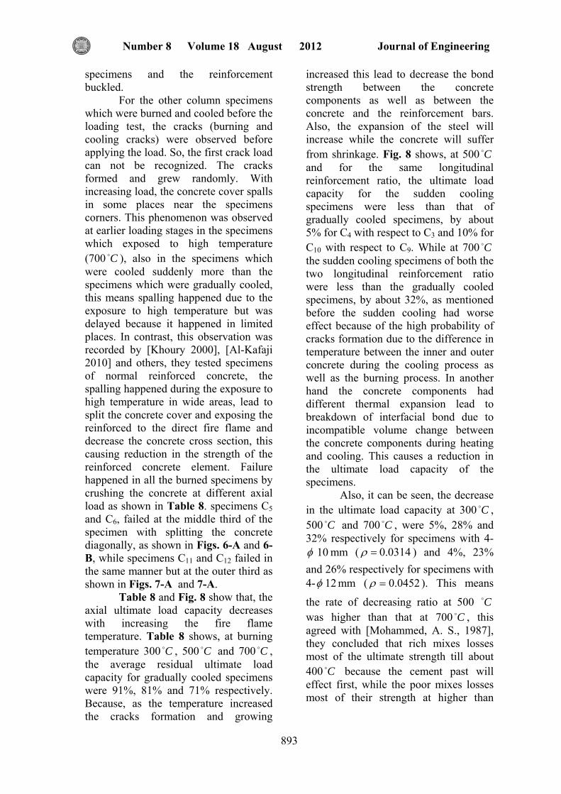
compressive strength was varying with the fire flame temperature as shown in Fig. 3, it decreases with increasing the exposure temperature. The average percentage of residual compressive strength after exposure to 300 Co , 500 Co

Effect of Fire Flame (High Temperature) on the Behaviour of Axially loaded Reinforced SCC Short Columns
Amer F. Izzat
[
892
and 700 Co was 82%, 65% and 43% respectively, for the specimens cooled gradually. The results agree with that obtained by other researchers for normal concrete, [Nevile and Brooks 1987] and [Al-Kafaji 2010]. The decrease in compressive strength of concrete is due to the breakdown of interfacial bond due to incompatible volume change between the concrete components during heating and cooling [Venecanin 1977]. While for the specimens which cooled suddenly (high rate of cooling), the residual compressive strength was slightly lesser than that, they were 61% 39% for the exposure temperature of 500 Co and 700 Co respectively. This may be due to the grading progression of decreasing temperature (cooling), which will never be uniformly through the concrete cross-section, because losing temperature will delay for the inner concrete than that of the outer concrete, this process will create internal damaged stresses, and it will be worse with increasing the cross-section of the concrete member. [Mohamedbhai 1986] conclusion's agreed with these results (for the normal concrete) till 500 Co but in contrast with that at 700 Co , his conclusion was, cooling rate affects on the residual concrete strength till 600 Co temperature, but it had no affect at more than this temperature, this may be because of using electrical furnace which can not allow to control the real cooling rate because of the delay time between the end of the exposure temperature and the cooling process i.e. no allowance to sudden cooling immediately after the exposure period.
Cracks due to burning: Cracks were observed on the
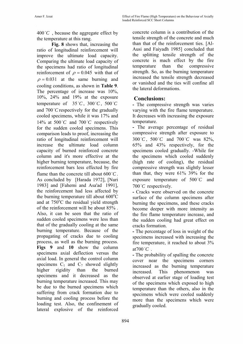
concrete surface of the column specimens after burning and cooling the specimens, and these cracks become deeper with more intensity as the fire flame temperature increase, as shown in Figs. 4-A and 4-B for columns C4 and C6
respectively. The column specimens which were exposed to 700 Co the concrete of the corners were split as shown in Fig. 4-B. This explains the decreases in the compressive capacity of the concrete with increasing the temperature. Comparing the formation of cracks in the two cooling conditions as shown in Figs. 4-B and 4-C, the sudden cooling in specimen C6 has greater effect on the cracks formation than specimen C5 which cooled gradually. This is because the rate of increasing temperature (according to the standard fire) ASTM E119-02 was less than that of decreasing temperature (sudden cooling), which had much worse effect on the interfacial bond between the concrete components. Also, the color of the concrete changes to pink, this may be due to hydration of iron oxide component and other mineral of cement and the aggregate [Al-Kafaji 2010] and [Neville 1995].
Fig. 5 shows the percentage of loss in weight versus the fire temperature, as shown in this figure the percentage of loss increased with increasing the fire temperature. [Mohammed 1987] recorded that till 300оC only the free water will be lost after that, the loss in weight caused by the chemical change in the aggregate properties. These two types of losses increase the cracks formation.
Mode of failure after the loading test: For the control column
specimens C1 and C2 few longitudinal fine cracks were observed at the outer thirds of the specimens, at about 105kN and 120kN respectively. With increasing load, new cracks were formed and the earlier cracks become wider. In general, the observed cracks were forming and progressed parallel to the longitudinal axis of the specimen then turned toward the edges of the cross-section. Failure occurred when the concrete crushed in one of the two outer thirds of the
Journal of Engineering Volume 18 August 2012 Number 8
893
specimens and the reinforcement buckled.
For the other column specimens which were burned and cooled before the loading test, the cracks (burning and cooling cracks) were observed before applying the load. So, the first crack load can not be recognized. The cracks formed and grew randomly. With increasing load, the concrete cover spalls in some places near the specimens corners. This phenomenon was observed at earlier loading stages in the specimens which exposed to high temperature (700 Co ), also in the specimens which were cooled suddenly more than the specimens which were gradually cooled, this means spalling happened due to the exposure to high temperature but was delayed because it happened in limited places. In contrast, this observation was recorded by [Khoury 2000], [Al-Kafaji 2010] and others, they tested specimens of normal reinforced concrete, the spalling happened during the exposure to high temperature in wide areas, lead to split the concrete cover and exposing the reinforced to the direct fire flame and decrease the concrete cross section, this causing reduction in the strength of the reinforced concrete element. Failure happened in all the burned specimens by crushing the concrete at different axial load as shown in Table 8. specimens C5 and C6, failed at the middle third of the specimen with splitting the concrete diagonally, as shown in Figs. 6-A and 6-B, while specimens C11 and C12 failed in the same manner but at the outer third as shown in Figs. 7-A and 7-A.
Table 8 and Fig. 8 show that, the axial ultimate load capacity decreases with increasing the fire flame temperature. Table 8 shows, at burning temperature 300 Co , 500 Co and 700 Co , the average residual ultimate load capacity for gradually cooled specimens were 91%, 81% and 71% respectively. Because, as the temperature increased the cracks formation and growing
increased this lead to decrease the bond strength between the concrete components as well as between the concrete and the reinforcement bars. Also, the expansion of the steel will increase while the concrete will suffer from shrinkage. Fig. 8 shows, at 500 Co and for the same longitudinal reinforcement ratio, the ultimate load capacity for the sudden cooling specimens were less than that of gradually cooled specimens, by about 5% for C4 with respect to C3 and 10% for C10 with respect to C9. While at 700 Co the sudden cooling specimens of both the two longitudinal reinforcement ratio were less than the gradually cooled specimens, by about 32%, as mentioned before the sudden cooling had worse effect because of the high probability of cracks formation due to the difference in temperature between the inner and outer concrete during the cooling process as well as the burning process. In another hand the concrete components had different thermal expansion lead to breakdown of interfacial bond due to incompatible volume change between the concrete components during heating and cooling. This causes a reduction in the ultimate load capacity of the specimens.
Also, it can be seen, the decrease in the ultimate load capacity at 300 Co , 500 Co and 700 Co , were 5%, 28% and 32% respectively for specimens with 4-
10φ mm ( 0314.0=ρ ) and 4%, 23% and 26% respectively for specimens with 4- 12φ mm ( 0452.0=ρ ). This means
the rate of decreasing ratio at 500 Co was higher than that at 700 Co , this agreed with [Mohammed, A. S., 1987], they concluded that rich mixes losses most of the ultimate strength till about 400 Co because the cement past will effect first, while the poor mixes losses most of their strength at higher than
Effect of Fire Flame (High Temperature) on the Behaviour of Axially loaded Reinforced SCC Short Columns
Amer F. Izzat
[
894
400 Co , because the aggregate effect by the temperature at this rang.
Fig. 8 shows that, increasing the ratio of longitudinal reinforcement will improve the ultimate load capacity. Comparing the ultimate load capacity of the specimens had ratio of longitudinal reinforcement of 045.0=ρ with that of
031.0=ρ at the same burning and cooling conditions, as shown in Table 9. The percentage of increase was 10%, 10%, 24% and 19% at the exposure temperature of 35 Co , 300 Co , 500 Co and 700 Co respectively for the gradually cooled specimens, while it was 17% and 14% at 500 Co and 700 Co respectively for the sudden cooled specimens. This comparison leads to proof, increasing the ratio of longitudinal reinforcement will increase the ultimate load column capacity of burned reinforced concrete column and it's more effective at the higher burning temperature, because, the reinforcement bars less effected by fire flame than the concrete till about 600 Co . As concluded by [Harada 1972], [Nuri 1983] and [Fahemi and Asa'ad 1991], the reinforcement had less affected by the burning temperature till about 600оC and at 750оC the residual yield strength of the reinforcement will be about 85% . Also, it can be seen that the ratio of sudden cooled specimens were less than that of the gradually cooling at the same burning temperature. Because of the propagating of cracks due to cooling process, as well as the burning process. Figs 9 and 10 show the column specimens axial deflection versus the axial load. In general the control column specimens C1 and C7 showed slightly higher rigidity than the burned specimens and it decreased as the burning temperature increased. This may be due to the burned specimens which suffering from crack formation due to burning and cooling process before the loading test. Also, the confinement of lateral explosive of the reinforced
concrete column is a contribution of the tensile strength of the concrete and much than that of the reinforcement ties. [Al-Ausi and Faiyadh 1985] concluded that the splitting tensile strength of the concrete is mach effect by the fire temperature than the compressive strength. So, as the burning temperature increased the tensile strength decreased or vanished and the ties will confine all the lateral deformations.
Conclusions: - The compressive strength was varies varying with the fire flame temperature. It decreases with increasing the exposure temperature. - The average percentage of residual compressive strength after exposure to 300 Co , 500 Co and 700 Co was 82%, 65% and 43% respectively, for the specimens cooled gradually. -While for the specimens which cooled suddenly (high rate of cooling), the residual compressive strength was slightly lesser than that, they were 61% 39% for the exposure temperature of 500 Co and 700 Co respectively. - Cracks were observed on the concrete surface of the column specimens after burning the specimens, and these cracks become deeper with more intensity as the fire flame temperature increase, and the sudden cooling had great effect on cracks formation. - The percentage of loss in weight of the specimens increased with increasing the fire temperature, it reached to about 3% at700 Co . - The probability of spalling the concrete cover near the specimens corners increased as the burning temperature increased. This phenomenon was observed at earlier stage of loading test of the specimens which exposed to high temperature than the others, also in the specimens which were cooled suddenly more than the specimens which were gradually cooled.

Journal of Engineering Volume 18 August 2012 Number 8
895
- The ultimate load capacity of the column specimens decreases with increasing the fire flame temperature, at burning temperature 300 Co , 500 Co and 700 Co , the average residual ultimate load capacity for gradually cooled specimens were 91%, 81% and 71% respectively. - Increasing the ratio of longitudinal reinforcement will enhance the residual load capacity. - Increasing the reinforcement ratio by 44% lead to increase the ultimate load capacity by 10%, 10%, 24% and 19% at the exposure temperature of 35 Co , 300 Co , 500 Co and 700 Co respectively for the gradually cooled specimens, while it was 17% and 14% at 500 Co and 700 Co respectively for the sudden cooled specimens. - for the same longitudinal reinforcement ratio, the ultimate load capacity for the sudden cooling specimens were less than that of gradually cooled specimens, by about 5% for C4 with respect to C3 and 10% for C10 with respect to C9. While at 700 Co the sudden cooling specimens of both the two longitudinal reinforcement ratio were less than the gradually cooled specimens, by about 32%. References: - Al Kafaji, M., 2010, " Effect of Burning on Load Carrying Capacity of Reinforced Concrete Columns", Ph.D. Thesis Presented to the University of Baghdad.
- Al Ausi, M.A., and Faiddh, F.I., 1985, "Effect of Method of Cooling on the Concrete Copmressive Strength Exposed to High Temperature", Engineering and Technology, Vol.1. –
- ASTM Designation C150-02"Standard Specification for Portland Cement " 2002 Annual Book of ASTM Standard, American Society for Testing and Material, Philadelphia Pennsylvania, Section 4,Vol. 4.02. PP 89-93.
- ASTM Designation C33-03"Standard Specification for Concrete Aggregate" 2002 Annual Book of ASTM Standard, American Society for Testing and Material, Philadelphia Pennsylvania, Section 4,Vol. 4.02. PP 10-16.
-ASTM Designation A615-05a"Standard Specification for Testing Method and Definitions for Mechanical Testing of Steel Products "2002 Annual Book of ASTM Standard, American Society for Testing and Material, Philadelphia Pennsylvania, Section 4,Vol. 1.01. PP 248-287C.
- ASTM Designation C143-03"Standard Test method of Hydaulic cement Concrete" 2003 Annual Book of ASTM Standard, American Society for Testing and Material, Philadelphia Pennsylvania, Section 4,Vol. 4.03. PP 1-4.
- ASTM Designation C33-03"Standard Specification for Concrete Aggregate" 2002 Annual Book of ASTM Standard, American Society for Testing and Material, Philadelphia Pennsylvania, Section4,Vol. 4.02. PP 10-16.
-ASTM Designation E119-01, "Standard Method of Fire tests of Building Construction and materials" 1987 Annual Book of ASTM Standard, American Society for Testing and Material, West Conshohocken .
-ASTM Designation E1611-05, "Standard Test Method for Slump Flow of Self Consolidated Concrete" 2005 Annual Book of ASTM Standard, American Society for Testing and Material, Philadelphia Pennsylvania, Section 4,Vol. 4.02.
- Fahemi, H. M., and Asa'ad, M. B., 1991, "Behavior and ultimate load capacity of reinforced concrete elements subjected to high temperature" journal of Building material Researches, University of Technology, Iraq, Vol. 10, No. 5. (paper in Arabic language)
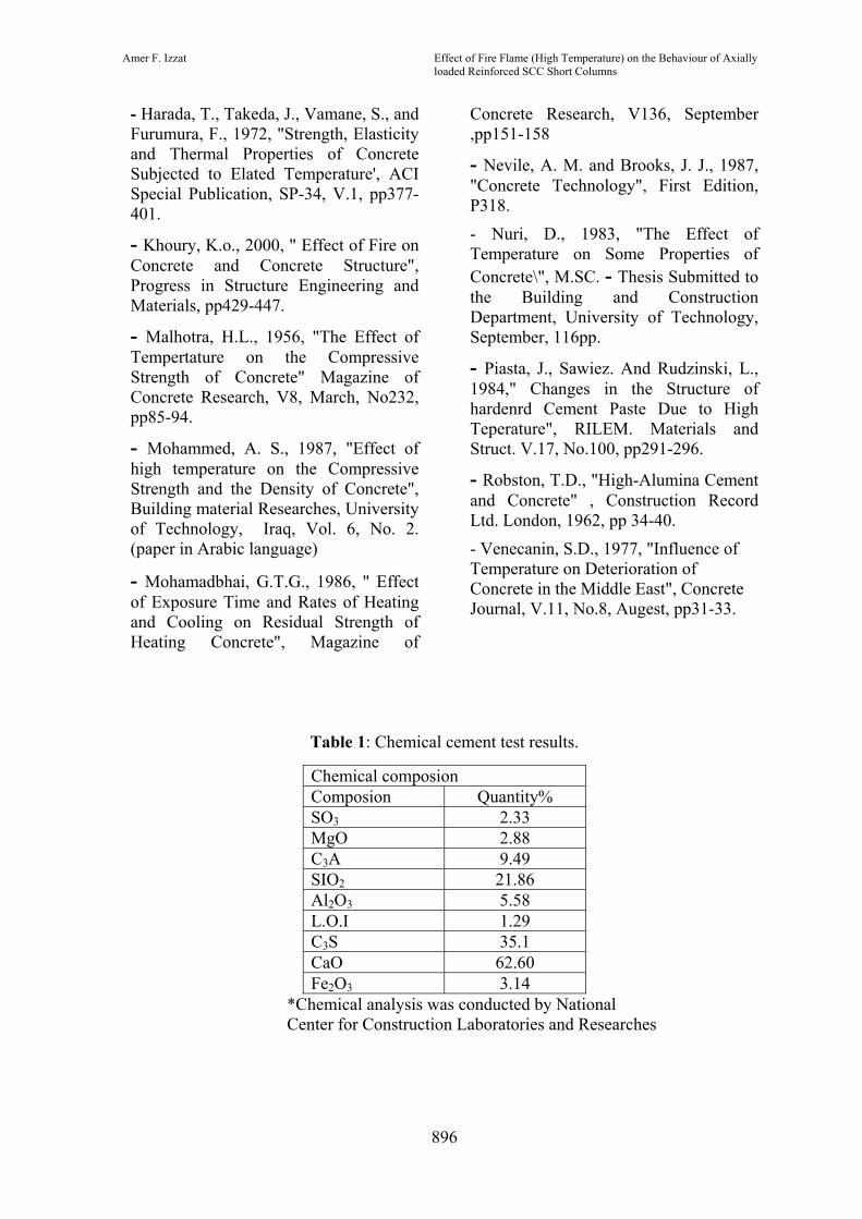
Effect of Fire Flame (High Temperature) on the Behaviour of Axially loaded Reinforced SCC Short Columns
Amer F. Izzat
[
896
- Harada, T., Takeda, J., Vamane, S., and Furumura, F., 1972, "Strength, Elasticity and Thermal Properties of Concrete Subjected to Elated Temperature', ACI Special Publication, SP-34, V.1, pp377-401.
- Khoury, K.o., 2000, " Effect of Fire on Concrete and Concrete Structure", Progress in Structure Engineering and Materials, pp429-447.
- Malhotra, H.L., 1956, "The Effect of Tempertature on the Compressive Strength of Concrete" Magazine of Concrete Research, V8, March, No232, pp85-94.
- Mohammed, A. S., 1987, "Effect of high temperature on the Compressive Strength and the Density of Concrete", Building material Researches, University of Technology, Iraq, Vol. 6, No. 2. (paper in Arabic language)
- Mohamadbhai, G.T.G., 1986, " Effect of Exposure Time and Rates of Heating and Cooling on Residual Strength of Heating Concrete", Magazine of
Concrete Research, V136, September ,pp151-158
- Nevile, A. M. and Brooks, J. J., 1987, "Concrete Technology", First Edition, P318.
- Nuri, D., 1983, "The Effect of Temperature on Some Properties of Concrete\", M.SC. - Thesis Submitted to the Building and Construction Department, University of Technology, September, 116pp.
- Piasta, J., Sawiez. And Rudzinski, L., 1984," Changes in the Structure of hardenrd Cement Paste Due to High Teperature", RILEM. Materials and Struct. V.17, No.100, pp291-296.
- Robston, T.D., "High-Alumina Cement and Concrete" , Construction Record Ltd. London, 1962, pp 34-40.
- Venecanin, S.D., 1977, "Influence of Temperature on Deterioration of Concrete in the Middle East", Concrete Journal, V.11, No.8, Augest, pp31-33.
Table 1: Chemical cement test results.
Chemical composion Composion Quantity% SO3 2.33 MgO 2.88 C3A 9.49 SIO2 21.86 Al2O3 5.58 L.O.I 1.29 C3S 35.1 CaO 62.60 Fe2O3 3.14
*Chemical analysis was conducted by National Center for Construction Laboratories and Researches

Journal of Engineering Volume 18 August 2012 Number 8
897
Table 2: physical cement test results Physical properties Compressive strength, MPa (3 days) (7 days)
23.46 28.80
Setting time (Vicate apparatus), Initial setting, h:min Final setting, h:min
2:50 4:15
Specific surface area (Blaine method), m2/kg
394
Soundness (Auto Clave ) method, %
0.10
*Physical tests was conducted by National Center for Construction Laboratories and Researches
Table 3: Chemical and physical gravel test results.
Properties Test results Absorption % 0.64 Specific gravity 2.62 Dry loose-unit weight kg/m3 1562 Sulfate content as SO3 % 0.05 Materials finer than 75µm% 1.36
* Tests was conducted by National Center for Construction Laboratories and Researches
Table 4: Chemical and physical sand test results. Properties Test results Absorption % 0.82 Specific gravity 2.49 Sulfate content 0.043
* Tests was conducted by National Center for Construction Laboratories and Researches
Table 5: Concrete mix proportions SCC Water Kg/m3 200 Superplasticizer lit./100Kg (powder) 3 Cement Kg/m3 392 Silica Fume Kg/m3 8 Total Powder Kg/m3 400 Gravel Kg/m3 640 Sand Kg/m3 600

Effect of Fire Flame (High Temperature) on the Behaviour of Axially loaded Reinforced SCC Short Columns
Amer F. Izzat
[
898
Table 6: Properties of steel bars
Bar diameter
(mm)
Yield stress
(MPa)
Strain at yield stress
(microstrain)
Ultimate stress (MPa)
3 10 12
542 512 504
2710 2497 2571
632 622 618
Table 7: Details of the columns specimens.
Column designation
Longitudinal reinforcement
Longitudinal Bar diameter
(mm)
Temperature C
Type of cooling
C1 4 - 10φ mm. 10 - - C2 4 - 10φ mm. 10 300 gradual C3 4 - 10φ mm. 10 500 gradual C4 4 - 10φ mm. 10 500 sudden C5 4 - 10φ mm. 10 700 gradual C6 4 - 10φ mm. 10 700 sudden C7 4 - 12φ mm. 12 - - C8 4 - 12φ mm. 12 300 gradual C9 4 - 12φ mm. 12 500 gradual C10 4 - 12φ mm. 12 500 sudden C11 4 - 12φ mm. 12 700 gradual C12 4 - 12φ mm. 12 700 sudden
* All specimens are made of SCC: self compacted concrete. ** Average concrete strength before burning was 35MPa for the cubes 100 x 100 x 100mm

Journal of Engineering Volume 18 August 2012 Number 8
899
Table 8 : Columns test results Column
designation Longitudinal Bar diameter
(mm)
Temperature
Co
Type of cooling
Ultimate load
capacity
Load capacity /reference column
% C1 10 - - 305 100 C2 10 300 gradual 290 95 C3 10 500 gradual 232 76 C4 10 500 sudden 220 72 C5 10 700 gradual 207 68 C6 10 700 sudden 142 46 C7 12 - - 335 100 C8 12 300 gradual 320 96 C9 12 500 gradual 287 86 C10 12 500 sudden 258 77 C11 12 700 gradual 247 74 C12 12 700 sudden 162 48
- Steel reinforcement ratio 0314.0=ρ for specimens with 4 - 10φ mm longitudinal bars - Steel reinforcement ratio 0452.0=ρ for specimens with 4 - 10φ mm longitudinal bars
Table 9: The effect of reinforcement on the percentage of the ultimate load capacity of
specimens had the same burning and cooling conditions Ratio of ultimate load capacity of
C7/C1 Gradually
cool
C8/C2 Gradually
cool
C9/C3 Gradually
cool
C10/C4 Sudden
cool
C11/C5 Gradually
cool
C12/C6 Sudden
cool Temperature Co 0 300 500 500 700 700
Percentage of increase
10% 10% 24% 17% 19% 14%

Effect of Fire Flame (High Temperature) on the Behaviour of Axially loaded Reinforced SCC Short Columns
Amer F. Izzat
[
900
A- Column cross-section B-Column dimensions
Figure 1 : Details of dimensions and reinforcement of concrete column specimens
B- Specimen positioning in the furnace
A- furnace with nozzles
Figure 2 : Details of furnace and the distribution of the nozzles and specimen position in the furnace during burning
Journal of Engineering Volume 18 August 2012 Number 8
901
Co
Co
0
10
20
30
40
50
60
0 200 400 600 800Temperature
Com
pres
sive
str
engt
h M
Pa
Gradually cooling condition
Sudden cooling condition
Figure 3: Effect of fire flame on compressive strength
A- Column specimen C4 after B- specimen C6 after C- specimen C5 after exposure to 500 Co and exposure to 700 Co and exposed to 700 Co and cooled suddenly cooled suddenly cooled gradually
Figure 4 : Cracks formation at different conditions of cooling and exposure temperature before the loading test
0
0.5
1
1.5
2
2.5
3
3.5
0 100 200 300 400 500 600 700 800
Temperature
% o
f los
s in
wei
ght
Figure 5: Effect of fire flame on the column specimens loss of weight
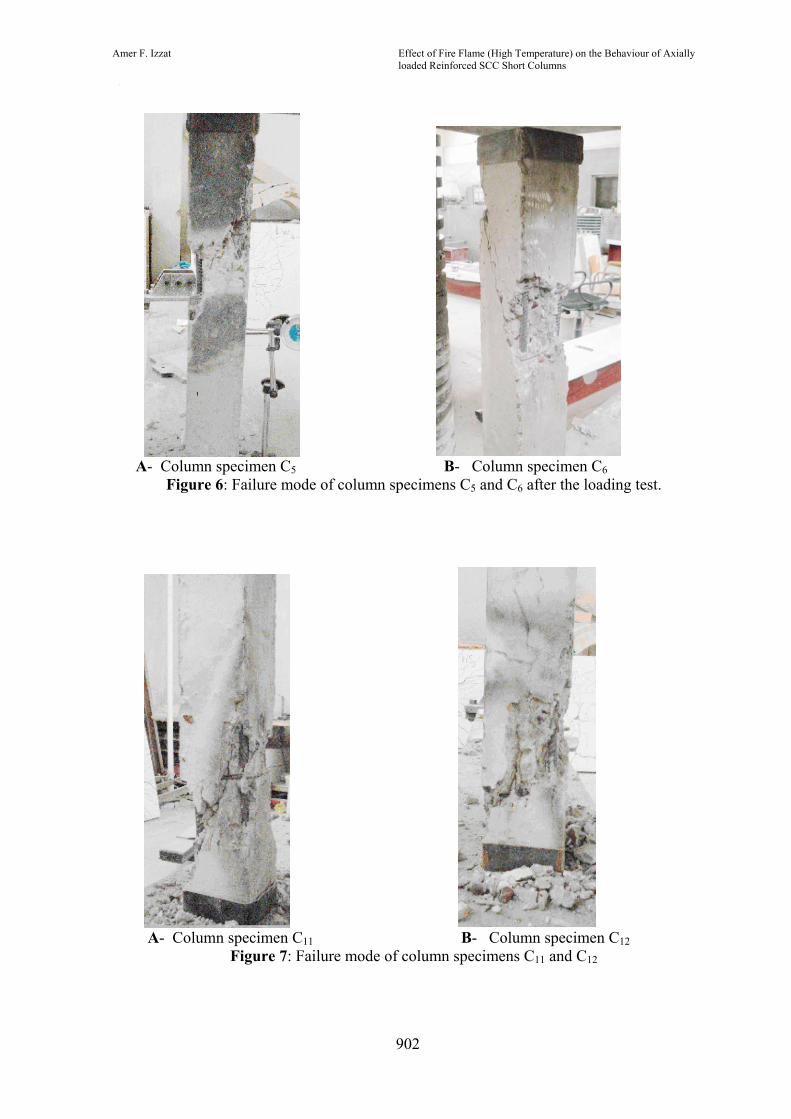
Effect of Fire Flame (High Temperature) on the Behaviour of Axially loaded Reinforced SCC Short Columns
Amer F. Izzat
[
902
A- Column specimen C5 B- Column specimen C6
Figure 6: Failure mode of column specimens C5 and C6 after the loading test.
A- Column specimen C11 B- Column specimen C12
Figure 7: Failure mode of column specimens C11 and C12

Journal of Engineering Volume 18 August 2012 Number 8
903
0
50
100
150
200
250
300
350
400
0 200 400 600 800
Temperature
Load
cap
acity
(kN
)
Columns with 10mm longitudenal reinf. -gradually cooled
Columns with 10mm longitudenal reinf. -suddenly cooled
Columns with 12mm longitudenal reinf. - graually cooled
Colmns with 12mm longitudenal reinf, - suddenly cooled
Figure 8 : Load capacity versus fire flame temperature
0
50
100
150
200
250
300
350
0 0.5 1 1.5 2 2.5Axial deformation (mm)
Axi
al a
pplie
d lo
ad
(kN
)
Column specimen C1Column specimen C2Column specimen C3Column specimen C5Column specimen C4Column specimen C6
Figure 9 : Applied axial load versus Axial deformation
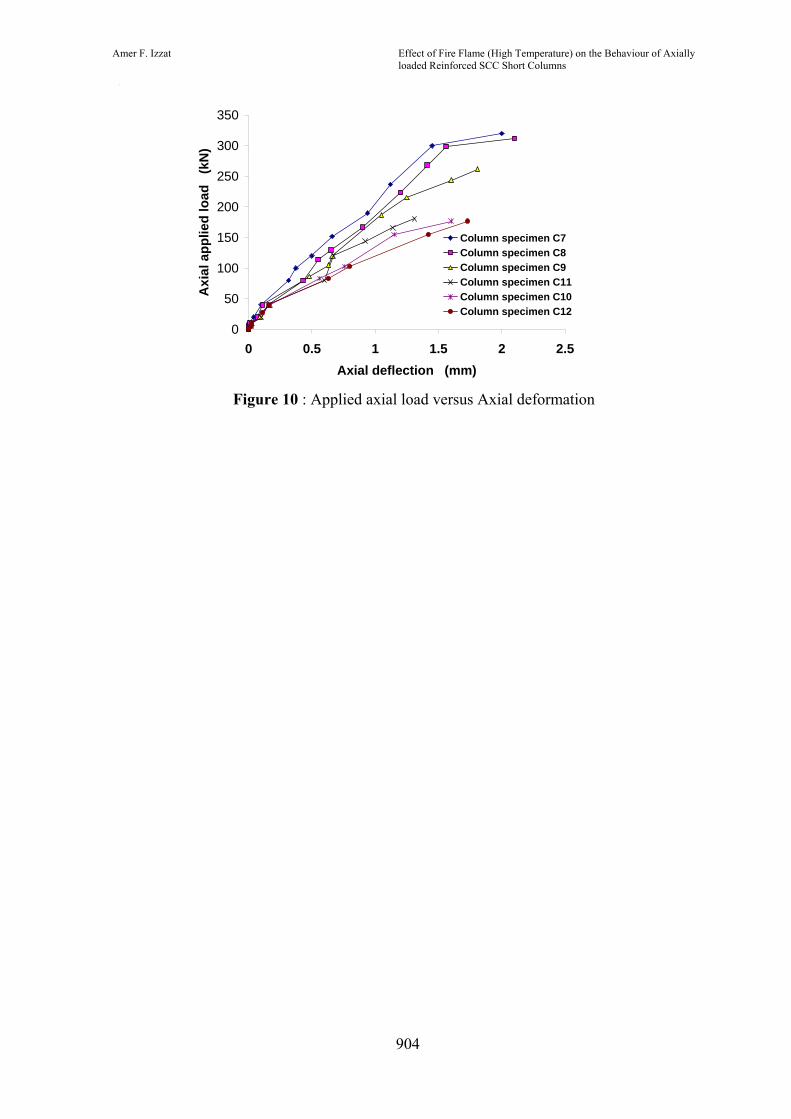
Effect of Fire Flame (High Temperature) on the Behaviour of Axially loaded Reinforced SCC Short Columns
Amer F. Izzat
[
904
0
50
100
150
200
250
300
350
0 0.5 1 1.5 2 2.5Axial deflection (mm)
Axi
al a
pplie
d lo
ad
(kN
)
Column specimen C7Column specimen C8Column specimen C9Column specimen C11Column specimen C10Column specimen C12
Figure 10 : Applied axial load versus Axial deformation

Journal of Engineering Volume 18 August 2012 Number 8 ج
905
Development A Method For Production Of Carbon Nanotubes
Dr. Mohamed.I. M*, Dr.N.J. Saleh*, L.H. Mohmood* Abstract In this work chemical vapor deposition method (CVD) for the production of carbon nanotubes (CNTs) have been improved by the addition of S. Steel mesh container (SSMC) inside which the catalyst (Fe/Al2O3) was placed. Scanning electron microscopy (SEM) investigation method used to study nanotubes produced, showed that high yield of two types of (CNTs) obtained, single wall carbon nanotube (SWCNTs) with diameter and length of less than 50nm and several micrometers respectively and nanocoil tubes with a diameter and length of less than 100nm and several micrometers respectively. The chemical analysis of (CNTs) reveals that the main component is carbon (94%) and a little amount of Al (0.32%), Fe (2.22%) the reminder is oxygen. It was also found that the use of (SSMC) leads to increase in yield by a factor of 3 of (SWNTs) and produces nanocoil at the same time. Keywords: Carbon Nanotubes (CNTs), Chemical Vapor Deposition (CVD), Stainless Steel Container (SSMC), Catalyst, C2H2.
آاربون النانو أنابيب النتاج طريقة تطوير
ةالخالص
من مصنوعة شبكية اويةح إضافة طريق عن النانوآاربون انابيب إلنتاج (CVD) الكيمياوي الكهربائي الترسيب طريقة تطوير البحث هذا في تم االلكتروني الماسح المايكروسوب تقنية استخدام أيضا تم. داخلها في (Fe/Al2O3) المساعد العامل وضع تم والتي (SSMC) للصدأ المقاوم الحديد
(SEM) الجدار أحادية يلي آما وهي العمل هذا في المنتجة الكاربون انابيب من نوعين وتشخيص للتعرف (SWNTs) 50 من اقل وطول روبقط واظهر. مايكروميترات بضع وبطول نانوميتر 100 من اقل وبقطر الحلزونية النانوية الكاربون وانابيب بالتتابع مايكروميترات وبضعة نانوميتر حديد%) 2,22(و لمنيوماأل %)0,32( و) بون آار% 94 (الكاربون هي األساسية مكوناته ان المنتجة النانوية الكاربون النابيب الكيمياوي التحليل النانوية الكاربون انابيب من مرات 3 مقدارها بزيادة الحصيلة زيادة الى ادت(SSMC) المستخدمة الحاوية ان وجد. األوآسجين هو والمتبقي .الوقت نفس في الحلزونية آاربون نانو انابيب إنتاج وآذلك
*University of Technology/Chemical Engineering Department/Baghdad/Iraq

Development A Method For Production Of Carbon Nanotubes
Dr. Mohamed. I. M Dr.N.J. Saleh L.H.Mohmood
906
Introduction Since the discovery of carbon nanotube in 1992(Iijima, 1991), an intensive research activity has been going on to improve methods and conditions, quality and productivity of carbon nanotubes (CNTs) (Zheng and Liu, 2000; Zeng et al., 2002) reaching rewarding conclusions. Due to their high strength, stiffness, and electrical conductivity, carbon nanotubes are designated as one of the most attractive materials for reinforcing the material in composite and nanoelectronic applications (Calvert, 1992; Mintmire et al., 1992; Hamada et al, 1992; Journet and Bernier, 1994). Among many methods of production (CNTs), the chemical vapor deposition (CVD) method is considered the most promising carbon nanotube production method in terms of industrial production (Tapas et al., 2005; Cinar and ruda, 2006). In principle chemical vapor deposition is achieved by the decomposition of hydrocarbon in the gas phase. Commonly used gaseous carbon sources include methane, carbon monoxide and acetylene with the aid of supported transition metal catalyst, (Ni, Fe, Mo, or Co). The (CVD) method is essentially a two - step process consisting of a catalyst preparation step followed by the actual synthesis of the (CNTs). The selection of a metallic catalyst may affect the growth and morphology of the nanotube. In the last few decades, different techniques have been developed for the carbon nanotube synthesis with (CVD). Most of research has been focused on improving the catalytic technique itself. Accordingly the main objective of the present work is to develop the
method of production of (CNTs) by using (CVD) techniques, and the products are identified by different identification techniques: Optical, scanning electron microscopy (SEM), and transmission electron microscopy (TEM). Experimental The experimental setup of (CVD) reactor which was used for fabrication of (CNTs) in this work is shown schematically in figure (1). The reactor consists of tubular furnace (a) in which quartz tube (b) of 900mm in length and (30) mm in diameter is placed horizontally in the tube furnace. Argon gas supplied from cylinder (C) is used as an inert gas. The hydrocarbon gas C2H2 is supplied by a cylinder (d) is used as a source of pyrolysis gas. In order to control the temperature microprocessor controller (e) is used. Preparation Of Catalyst (6%) of Fe2O3 was blended with (10%) solution of novalac in (90) ml of ethanol. Then a thin film of previous blended mixture was painted on alumina substrate. The substrate was dried in oven at (400)0C for one hour. Ten pieces of substrate of (10) mm length and (5) mm diameter were placed inside a cylindrical shape S. Steel mesh container (SSMC) of (200) mm length and (20) mm in diameter. The (SSMC) was then placed inside the quartz tube furnace. PREPARATION OF (Cnts)

Journal of Engineering Volume 18 August 2012 Number 8 ج
907
A catalytic growth of (CNTs) was carried out by the decomposition of acetylene C2H2 at temperature (700)0C for o.5h by introducing a mixture of (C2H2/Ar) (50ml/500ml) into the reactor. Finally, the gas flow was switched back to Ar and the furnace was allowed to cool to room temperature before exposing the product to the air. Samples of (CNTs) were allowed to grow without (SSMC) so that the effect of (SSMC) on the yield of (CNTs) would be investigated. The (CNTs) yield (y) was roughly calculated as follows eq. (1):
( )( )mgB
mgmgmgy C0)/( = (1)
Where (C0) is the weight of as prepared product sample mg and (B) is the weight of the catalyst precursor Fe2O3/Al2O3 mg. . Characterization Scanning Electron Microscopy (SEM) A Carl Zeiss-Supra with accelerator voltage 5KV (UKM Malaysia) was A Carl Zeiss-supra with accelerator voltage 5 Kv (UKM Malaysia) was employed to observe the structure of carbon nantube. (XRD) pataren of CNTS was record using Standard Phillips type PW1877 Automated powder diffractometer was used with Cu-Kα radiation and a pure Silicon powder as a standard employed to observe the structure of carbon nanotubes.
Results And Discussion Two type of experiments were carried out, the first with fixed flow rate of Argon fixed as a carrier gas using different reaction temperatures, fixed reaction time and substrate enclosed in (SSMC) container. In the second experiment (SSMC) was eliminated, fixed reaction time and optimum temperature was obtained from the first set of experiment in which a high yield of (CNTs) was obtained for the first set of experiments with Ar fixed as carrier gas. The total amount of (CNTs) deposited on the catalyst after reaction was determined by weight gain in the tube in furnace during the reaction. The influence of the reaction temperature on (CNTs) yield with and without (SSMC) is shown in figure (2). It can be observed that the yield of (CNTs) produced at 4000C is very low, with the increase in reaction temperature, the yield is increased rapidly, but when the reaction temperature is increased to 700 0C, the yield begins to decrease. This may due to the fixed flow rate of argon gas which may cause the oxidation some of the produced (CNTs) after 7000C and converted to CO2. Similar behavior was obtained without using (SSMC) but with a lower yield. The yield gain is increased by a factor of 3 when (SSMC) is used. The (SEM) results are shown is figures (3-6). It is well known that it is difficult to decide from diameters measured by SEM whether a nanotube is single wall or not (Tapas et al., 2005; Cinar and ruda, 2006). It is only used to estimate the tube diameter. Our observation suggest that the product is (SWNTs) rather than (MWNTs). The carbon nanotubs

Development A Method For Production Of Carbon Nanotubes
Dr. Mohamed. I. M Dr.N.J. Saleh L.H.Mohmood
908
shown in scanning electron microscopy (SEM and TEM) images shown in figures (3-6) were synthesized at high yield in two types: Single wall nanocarbon tubes with characteristic diameter (20- 40 nm) and nanocarbon coils. The diameter and length of (SWNTs) are less than 50nm and several micrometers, respectively, while the nanocoil diameter and length are less than 100nm and several micrometers respectively. Our observation suggests that the (SWNTs) grow as a result of using (Fe/Al2O3) catalyst while nanocoil is identified when (SSMC) was used. Accordingly the use of (SSMC) leads to increase in yield of (SWNTs) and produces a nanocoil at the same time. The high yield observed when using (SSMC) may be attributed to the effect of (SSMC) on slowing down the velocity of C2H2 gas, which may give more chance to gas to decompose in high yield through the tube reactor. Moreover the (SSMC), a stainless steel type 316L consists of different elements Cr(16-18%), Ni (10-19%), Mn (2%), Si (1%) and other traces elements (P,S,C). These elements are deoxidized by carbon and hydrogen of C2H2 at high temperature 7000C and then they may absorb carbon to form crystalline Fe-Cr-Ni-Mn carbide compounds. On which a nanocoils form crystalline compounds. The spectrum in Figure (7) represent the chemical analysis of the (CNTS) sample obtained by electron diffraction spectroscopy (SDS) of SEM system showing the majority are carbon (94%) and a little amount of Al (0.32%) and Fe (2.22%) and the remainder is oxygen formed (3.33%). Figure (8) shows the (XRD) spectra of (Fe/SSMC) catalyst.
Many peaks observed which may be attributed to graphite and Fe these peaks may be corresponding to the formation of metal carbides. This suggestion agrees well with conclusion drawn by (Kenji et.al, 2004) based on similar observation. Conclusion The (CVD) method of production of (CNTs) has been improved by adding (SSMC). The (SSMC) is responsible for high yield production of (CNTs). (SSMC) may also be responsible for growth of carbon nanocoil, in this case we believe that Iron is oxidized and catalyst form nanoparticles by heating to a growth temperature of 700 oC in Ar atomosphere. The nano particles contain nanocrystal of Iron oxide and other element oxides, suppling of C2H2 gas may deoxidize the catalyst and then carbon atoms be incorporated into the catalyst form crystalline carbide compounds, carbon nanocoils may be grown form these crystalline compounds. Symbols list B: the weight of the catalyst precursor Fe2O3/Al2O3 mg. C0: the weight of as prepared product sample. CVD: Chemical Vapor Deposition Method. CNTs: Carbon Nanotubes. SEM: Scanning Electron Microscopy. SSMC: Stainless Steel Mesh Container SWCNTs: Single Wall Carbon Nanotube. SDS: Electron Diffraction Spectroscopy.
Journal of Engineering Volume 18 August 2012 Number 8 ج
909
TEM: Transmission Electron Microscopy.
Y: yield. References Calvert, P. Strength in Disunity. Nature, 357: 365, (1992). Cinar, O. and ruda, y. Carbon Nanotube Synthesis via the Catalytic CDV Method, Areview on the Effect of Reaction Parameters. Fullerenes, Nanotubes, and Carbon Nano structures, 14: 17-37, (2006). Hamada, N., Sawada, S., and Oshiyama, A. "New One – Dimensional Conductors: Graphitic Microtubules". Phys. Rev. Lett., 68: 1579, (1992). Iijima, S. "Helical Microstructure of Graphitic Carbon Nature", 354: 56, (1991). Journet, C. and Bernier, P. "Production of Carbon Nanotubes". Appl. Phys. A, 67: 1, (1994). Kenji, N, Lujun, P. and Yoshikazu, N., "In Situ Study of Fe/ITO Catalysts for Carbon Nanocoil Growth by X-ray Diffraction Analysis". Japanese J. of Appl. Phys. A, 8:43, pp 5665-5666. (2004). Mintmire, J. W., Dunlap, B. L., and White, C.T. are Fullerene Tubules Metallic. Phys. Rev. Lett, 68: 631, (1992).
Tapas L., Kertesz K., Vertesy Z., Horvath Z. E., Koos A. A, Z.Osvath, ZS. Sarkozi, Al. Darbont, L. P. Biro., "Diameter and Morphology Dependence on Experimental Conditions of Carbon Nanotube Array Arown by Spray Pyrolysis"Carbon 43 970- 977, (2005). Zeng, X., Cheng, G., Yan, X., and Xu, "Production of Multi- Wall Carbon Nanotubes on a Large Scale". Physical B, 323: 330, (2002). Zheng S. and Liu J. "A scalable CVD Method for The Synthesis of Single – Walled Carbon Nanotubes with High Catalyst Productivity". Chem. Phys. Lett., 322: 321, (2000).

Development A Method For Production Of Carbon Nanotubes
Dr. Mohamed. I. M Dr.N.J. Saleh L.H.Mohmood
910
Fig.1: (CVD) Experimental Setup: (a) Tubular Furnace (b) Quartz tube (c) Argon Gas
Cylinder (d) Acetylene Gas Cylinder (e) Furnace Controller
Fig.2: Effect on Reaction Temperature on the Yield of (CNTs)
Ar
C2H2
Q SSMC
Trap
b
e
a
c d
0
0.5
1
1.5
2
2.5
450 500 550 600 650 700 750 800
Temperature of reactor C
Yiel
d (m
g/m
g)
With CSSC
Without CSSC

Journal of Engineering Volume 18 August 2012 Number 8 ج
911
a: with
(SSMC), b: without (SSMC)
Fig.3: SEM Image of (SWCNTs)
Fig. 4: SEM Image of (SWCNTs)

Development A Method For Production Of Carbon Nanotubes
Dr. Mohamed. I. M Dr.N.J. Saleh L.H.Mohmood
912
Fig.5: TEM image of (SWNTs)
Impurities (catalyst)
Fig.6: SEM Image of Nanocoil
Journal of Engineering Volume 18 August 2012 Number 8 ج
913
Fig.7: Chemical Analysis of (CNTs)
Fig.8: XRD of (SSMC) after Heated at 700oC in (CVD) Reactor
600
400
200
0
0 20 40 60 80
Journal of Engineering Volume 18 August 2012 Number 8
914
Spectral Technique for Baud Time Estimation Mohammed K. Al-Haddad Dr. Sarcout N. Abdullah Prof. Qais S. Ismail. Electronics and Comm. Dpt. Electronics and Comm. Dpt. Computers Dpt. Baghdad University Baghdad University Baghdad University ABSTRACT A new approach for baud time (or baud rate) estimation of a random binary signal is presented. This approach utilizes the spectrum of the signal after nonlinear processing in a way that the estimation error can be reduced by simply increasing the number of the processed samples instead of increasing the sampling rate. The spectrum of the new signal is shown to give an accurate estimate about the baud time when there is no apriory information or any restricting preassumptions. The performance of the estimator for random binary square waves perturbed by white Gaussian noise and ISI is evaluated and compared with that of the conventional estimator of the zero crossing detector. Key words- Bit time estimation, baud time estimation, bit rate estimation, baud rate estimation.
الخالصةهذا االسلوب يعتمد على طيف االشارة بعد معالجتها بصورة غير خطيـة ). او معدل الترميز( لتقدير زمن الترميز اسلوب جديد تم اعتماد
ارة الجديدة اظهـر ان طيف االش . بحيث يمكن تقليل خطأ التقدير عن طريق زيادة عدد العينات المعالجة بدالً من زيادة معدل اخذ العينات
أظهر التقييم ألداء لعملية التقدير الشارة ثنائية عـشوائية مـضافاً اليهـا . تقدير دقيق لمعدل الترميز من دون معلومات او فرضيات مسبقة
.الضوضاء الكاوسي والتداخل الرمزي وُأجريت مقارنة مع طريقة كشف التقاطع الصفري
INTRODUCTION Many researches have been made for identifying the type of modulation of the unknown signal, now the interest is moved one step ahead to the estimation of the baud rate (or baud time) of the unknown signal. The estimation of the baud rate can be used with information obtained from the modulation identification to provide better knowledge about the characteristics of the signal, this sometimes referred to as signal identification [1, 2]. Besides that the knowledge of the baud rate is needed if the information contained in the unknown signal is to be extracted, since the baud rate is required for the timing recovery block of the demodulator. If the technique used for the clock recovery is PLL based, the baud rate is used to specify the center frequency of the VCO or if the spectral line technique is used, the baud rate is used to determine the center frequency of the BPF [5]. The quality of the baud time estimator is generally measured by the following criteria [1]:
1- The amount of available apriory information. The less information available the better the system is. 2- Time taken for the baud rate estimation or it can be measured as the amount of computation. 3- The accuracy of the estimation. Several techniques have been developed for estimating the baud time, most of the techniques presented in the literature analyze the zero-crossing of the baseband signal. Wegener [1] presented detailed description of different approaches that rely on the zero crossings of the signal and no performance evaluation was presented. Gaby [2] presented an algorithm that relies both on zero-crossing and bit pattern analysis and he used second derivative of the filtered modulating signal to locate the baud transitions which is more general than the zero crossing because it works for the multilevel signaling. The second derivative helps locating the inflection point of smoothed (filtered) signal which is actually the baud transition point. Azzouz [3] used wavelet transform in his work and he also relied on the zero-
Spectral Technique for Baud Time Estimation
Mohammed K. Al-Haddad Dr. Sarcout N. Abdullah Prof. Qais S. Ismail.
ج
915
crossings of the signal and he used the derivative if the signal to enhance the part of the signal where the zero-crossing occurs. Scheets [4] have used adaptive filtering of the random binary signal and monitored the coefficients of the adaptive filter, which gave the estimation of the bit time of the binary signal. His work was compared to the zero crossing method for estimating the bit time. Sills [5] developed an algorithm based on histogram of baud transition. Boulinguez [6] approach is based on time-frequency representation of the modulated signal combined with periodicity analysis using Kalman filter. These works although differ in the details of their approaches but they all share the same limitation of having their analysis in the time domain, such approach will limit the accuracy of the estimation by the choice of the sampling frequency as will be explained later. If high accuracy is needed the ratio of sampling frequency to the baud rate should by be high enough. This indicates the need of having apriory information available for estimating the baud rate. Also if filtering is used, the choice of the cutoff frequency will raise the same issue. In the proposed approach it is assumed that no apriory information available and the approach is developed to depend on the spectrum of a non-linear processed version of the input signal. This nonlinear processing introduces impulses at multiples of the baud rate in the spectrum, and by identifying the position of these impulses the baud rate or baud time is estimated. Very high estimation accuracy can be obtained about the value of baud time Tb when high resolution of the spectrum is available which is achieved by simply increasing the amount of the processed samples for the same sampling frequency. The quality of the spectral estimator is compared to that of the conventional estimator based on generating histogram (clusters) of the zero crossings [1], [2]. The analysis will be presented for a two levels (M=2) and four levels (M=4) signals. For simplicity of explanation of the approach, the two level signaling will be considered and the terms bit time and bit rate will be used rather than baud time and baud rate. The algorithm that will be presented works perfectly on the multilevel signals (M>2) without any modifications.
Effect of Sampling Frequency on Bit Time Estimation Before starting with the details of the spectral estimator, it is useful to elaborate about the sampled signals bit time. In sampled data domain, the time is represented by samples rather than seconds because
the time is quantized to sampling intervals or sample time Ts given by
sf1T =s (1)
Where fs is the sampling frequency in samples/sec. Therefore any time-related information, like the bit time, is given in terms of number of samples. In other words the bit time will be represented as multiple of Ts. According to above, the bit time in the sampled data domain can be found by [1]
s
b
TTT = (2)
Where,
- Tb is the bit time in seconds - Ts is the sample time in sec/sample - T is the bit time in samples
Or
b
s
RfT = (3)
Where, Rb is the bit rate. According to eq. (3) T may not be an integer only if the sampling rate is an integer multiple of the bit rate and since the bit rate is unknown, actually the problem here is to estimate the bit rate, we cannot assume T an integer. As mentioned earlier, previous works relied on time domain processing of the signal. The disadvantage of a time domain approach is that the need of high sampling frequency compared to the bit rate. The reason of that is illustrated in Fig. 1, where in Fig. 1a a sampled binary signal is shown, its bit time T=12 samples. In Fig. 1b the same signal is sampled with a half the sampling frequency of the one in Fig. 1a which made the bit time T=6 samples. In case (b) the quantization of time is not as fine as in case (a), therefore the estimation of the bit time in case (b) will be less precise than case (a). In Fig. 1c another binary signal is shown with bit rate twice as much as in case (a) and sampled with the same sampling frequency, which made the bit time T=6 also. So, to have the same estimation precision as in case (a) the sampling frequency needs to be doubled. In summary the estimation of bit time in time domain raises the problem of having the estimation accuracy dependant on the sampling frequency. It will be explained that using the frequency domain feature of the signal does not make high values of the sampling frequency a requirement for the estimation precision.

Journal of Engineering Volume 18 August 2012 Number 8
916
Spectral Properties of Random Binary Signal In this work the estimation of the bit time is based on the frequency domain as a feature of the signal. The spectrum of the signal gives an idea about the bit time because it is directly affected by the bit time. For example the power spectral density (psd) of a random binary (non-return to zero) signal x(t) is in the form of the well known sinc function [8].
22
2/)2/sin()( ⎥⎦
⎤⎢⎣
⎡=
b
bbx T
TTASω
ωω (4)
It is clear from eq. (1) that the bit time Tb shrinks or spreads the spectrum according to its value. Moreover this spectrum contains nulls (zero values) at multiples of the bit rate (the reciprocal of the bit time). But unfortunately, this form of spectrum can only give a rough estimate about the bit time, mainly because of the difficulty of locating the nulls in the presence of noise.
In Fig. 2a and 2b the spectrum of a random binary signal with SNR equals to 100 dB and 10 dB is shown. It is possible to estimate the bit rate (and hence the bit time) if the first null is located, but due to the presence of noise, the exact location of the null is lost. This is expected since the noise mostly affects the small values of the spectrum. To tackle this problem, the proposed approach is to introduce impulses (or spectral line) at the locations of the nulls, because the impulses are easier to locate and more immune to noise. But the spectrum of random binary signals of most formats do not contain these impulses, actually the impulses in the spectrum is a characteristic of a periodic signal [8,9]. To introduce these impulses into the spectrum of the binary signal we first need to look at the spectrum of the general random binary signal f(t) with the following properties [8]
1. Each pulse is of Tb duration. 2. The two possible states in each interval are represented by the waveforms f1(t) and f2(t) with corresponding Fourier transforms F1(ω) and F2(ω). 3. The probability that f1(t) is selected in any interval is p and the probability that f2(t) is selected is q=(1-p). 4. The choice of f1(t) and f2(t) in any interval is statistically independent of that in any other interval. The psd of such signal is given by
∑∞
−∞=
−−+
+−−=
nbbb
b
bf
nnFpnpFT
FFT
ppS
)()()1()(2
)()(1)1()(
212
221
ωωδωωπ
ωωω (5)
Where, ωb=2π/Tb. The second term of eq. (5) can be used to estimate the bit rate (and hence bit time) because it is in the form of impulses at multiples of bit rate that can be easily detected even in the presence of noise. To have this term produced when p=q=0.5, two conditions should be satisfied F1(ω) ≠ –F2(ω) (6a) F1(nωb) ≠ 0 and F2(nωb) ≠ 0 (6b) The first condition to make F1(ω) and F2(ω) do not cancel each other, and the second condition is to make the weight of the impulses nonzero. Now if we consider the usual case of the binary signal where f1(t)= A and f2(t)= −A and the both cases are equally likely to occur (p=0.5). It is clear that the first condition is not satisfied (and it can be shown that the second is also not satisfied). Therefore, the impulses term vanishes in the spectrum of such signal and strictly speaking, for this case eq. (5) will be reduced to eq. (4). Proposed Spectral Approach for Bit Time Estimation To introduce the impulses term of eq. (5) we need to modify the signal f(t) in such a way that the two conditions given by eq. (6) are satisfied. There is no unique way to modify the signal f(t) in order to satisfy these conditions. The approach introduced in this paper is to differentiate the signals and taking the absolute value (a different approach can use squaring instead of absolute value). The new signal g(t) will have the conditions of eq. (6).
dt)t(df)t(g = (7)
g(t) is now in the form of positive impulses at every bit change of f(t) and zero elsewhere, as shown in Fig. 3. It can be seen that g(t) has all the above mentioned properties with g1(t) = 2Aδ(t) (8a) g2(t) = 0 (8a)

Spectral Technique for Baud Time Estimation
Mohammed K. Al-Haddad Dr. Sarcout N. Abdullah Prof. Qais S. Ismail.
ج
917
with Fourier Transforms G1(ω) = 2A (9a) G2(ω) = 0 (9b) It can be seen that G1(ω) and G2(ω) satisfy the two conditions in eq. (6). From eq. (5) and eq. (9) the psd of g(t) is
∑∞
−∞=
ω−ωδπ
+=ωn
b2
bb
2
g )(AT2
TA)(S (10)
This proposed approached has made the new signal g(t) in a way that the value of the spectral component at the bit rate frequency as high as possible (impulse), instead of zero as it was in the case of f(t) before processing. The impulses of the spectrum of g(t) can now be detected even in the presence of noise (as shown in Fig. 4), because the effect of noise on the spectral component of the bit rate of g(t) will be much less than the noise effect on the zero (null) value for the same spectral component of f(t). This will make it much easier to detect this impulse, and from its location the bit time can be estimated
Development of the Estimator for the Sampled Signals As explained earlier, in the sampled data domain the bit duration is represented by the number of samples per bit T, where T can be obtained by eq. (2) and eq. (3), note that T may not be an integer. Now the signal in question f(t) will be represented after sampling as f(n). From this sampled signal the formula of eq. (7) will be in the form
)1n(f)n(f)n(g −−= (11) In sampled data domain the differentiation is replaced with difference [9, 10]. This processing is adequate at high values of signal-to-noise ratio, but at low values of signal-to-noise ratio the time domain impulses created at the bit changes may not be so distinct because they come as the difference of two samples only. An alternative and more practical modifying formula is
( )∑=
−−−−−=L
0i)1Lin(f)in(f)n(g (12)
Note that eq. (11) is a special case of eq. (12) for L=0. This formula takes a window of 2(L+1) samples and sums a group of (L+1) consecutive samples and
the group of the next (L+1) consecutive samples and takes the difference between the two sums. This produces some averaging of the noise and hence reducing its effect. Besides the time-domain impulses will have a non-zero width which in turn makes the frequency-domain impulses have a decreasing weight [8]. This makes it easier to detect the impulse at ω=ωb (which will be referred to as the bit rate impulse) as the largest impulse other than that at ω=0. Now the spectrum of g(n) can be obtained using Fast Fourier Transform (FFT) and it will be denoted by G(k) where k is the frequency index. Since G(k) is defined over discrete values of the spectrum and the bit rate (or bit time) has a continuous range of values, the bit rate impulse would not appear exactly at one of these discrete values except for the special case where[9]
kf
NR
s
b = (13)
where N is the number of FFT points and k is any integer. If this expression is not satisfied, which is usually the case, the impulse will be split into two impulses at successive values of the frequency index k. Let these two values of k be kb and kb+1, the estimate of the impulse location bk can be obtained as the weighted average of kb and kb +1 with G(k) and G(k+1) as their weights respectively, i.e.
)1()()1()1()()(
++
+++=
bb
bbbbb kGkG
kkGkkGk (14)
The estimate of the number of samples per bit is obtained by
bkNT = (15)
This equation, despite its simplicity, has a very interesting feature. As has been explained earlier in section 1, the bit time T cannot necessarily be an integer value, and that the precision of time domain approach for the bit time estimation can only be enhanced by increasing the sampling frequency. Equation (15) is telling us that the estimate of the bit time is the ration of two numbers, one is the number of the processed samples N and the other is the frequency index bk . It is clear that the value of a non integer number is better approximated by the ratio of large integers, which is the case for eq. (15) when N is increased. This is when compared with the time domain approach is a very big advantage because to

Journal of Engineering Volume 18 August 2012 Number 8
918
have a better estimation precision in the frequency domain approach, it only requires to increase the number of the processed samples as will be seen in the results presented in the next section, which is a much easier condition to satisfy than increasing the sampling rate, which usually a hardware requirement.
Performance Evaluation against Awgn and Isi The estimator performance against band limited channel and AWGN is to be investigated now. A random binary signal of 15 kb/s bit rate is simulated and sampled with a sampling frequency of 100 ksample/s, this makes T=6.667 samples/bit. This choice of values was to show that in presented approach there is no need to have high values of T in order to have good estimation accuracy unlike other works were the choice was T=30 in [4] and T=96 in [3]. Also our choice of is T is a non-integer value to avoid any loss of generality. Channel and noise model in continuous time is in the form
∫ +−= )()()()( tndtshtf τττ (16)
Where s(t) is the baseband transmitted signal that is assumed to be a rectangular NRZ signal since this format is the most widely used format, h(t) is the combined impulse response of the transmitter filter, channel filter and the receiver filter, which is responsible for introducing the intersymbol interference (ISI) into the received signal. The term n(t) is the AWGN, and the signal-to-noise ratios is defined in terms of SNR per bit [4] where
n
s
n
ss
PTP
RPfPSNR == (17)
Ps and Pn are variances of the signal and noise samples, respectively. Equation (17) reflects more accurately the noise power inside the signal bandwidth than the standard SNR=Ps/Pn. The effect of transmission over a band limited channel is important in the evaluation of this work not only because it is a practical factor that affects most of the communication systems, but it also affects the shape of the transmitted pulse. And since our work depends mainly on the wave shaping, it is expected that the performance would be degraded by the presence of the band limiting (or ISI) because it is expected to soften the sharp edges of the transmitted rectangular pulse. In simulation, eq. (16) needs to be transformed into sampled data format
∑=
+−=K
k
nnknskhnf0
)()()()( (18)
Where n is the time index and K is the total number of samples of the combined impulse response h(n) which is referred to as the channel memory. The summation in eq. (18) represents the weighted sum of the delayed versions of the transmitted signal s(n), it should be noted that in some literatures, the discrete nature of eq. (18) comes from sampling the signal with sampling rate equals the symbol rate, i.e., one sample per symbol, this means that the delay of s(n) only occurs at multiple of the symbol time, which is generally not the case. In our work the summation of (18) is of the samples of the signal due to the sampling rate mentioned earlier which is greater than the symbol rate, i.e., more than one sample per symbol and that the delays occur at fractions of the symbol time. This representation of the ISI is more practical and will affect the value of the transmitted symbol as well as the shape of the wave of the symbol, unlike the one sample per symbol model that only affects the value of the transmitted symbol only. In regards to the amount of the ISI introduced by the channel, the value of the channel memory K is sometimes used, but this is not an accurate measure because the values of h(k) are not considered. A more informative parameter is the channel bandwidth, since the channel effect is band limiting and our signal s(n) is a baseband signal h(n) is chosen as an FIR LPF and its bandwidth will be the measure adopted here for the amount of ISI in our simulation. The number of taps K of the FIR LPF is chosen to be 101, and considering the value of T=6.667, this is equivalent to about 15 symbols interference. Hanning window is chosen and the results were obtained for different values of the cutoff frequency which is expressed as a relative frequency or digital frequency given by
sffr = (19)
Note that comparing the above equation with eq. (2), it defines the digital frequency corresponding to the baud rate as 1/T which for our case is 0.15. Fig. 5 shows an example of a signal in three conditions; the clean signal, signal with ISI and the signal with ISI and noise. The spectrum of the signal g(n) is estimated using the periodogram averaging method [10]. It was found that the number of 10 periodograms which is a convenient number to avoid increasing the number of calculations and it was found sufficient to produce very acceptable results The results are obtained for standard deviation or root mean square (RMS) of the estimation error given by
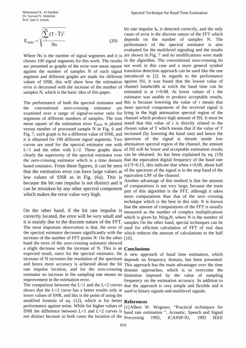
Spectral Technique for Baud Time Estimation
Mohammed K. Al-Haddad Dr. Sarcout N. Abdullah Prof. Qais S. Ismail.
ج
919
Ns
)T-T(E
Ns
1
2
RMS
∑= (20)
Where Ns is the number of signal segments and it is chosen 100 signal segments for this work. The results are presented as graphs of the error root mean square against the number of samples N of each signal segment and different graphs are made for different values of SNR, this will show how the estimation error is decreased with the increase of the number of samples N, which is the basic idea of this paper. The performance of both the spectral estimator and the conventional zero-crossing estimator are examined over a range of signal-to-noise ratio for segments of different numbers of samples. The root mean square of the estimation error ERMS is plotted versus number of processed sample N in Fig. 6 and Fig. 7, each graph is for a different value of SNR, and it is obtained for 100 different signal segments. Two curves are used for the spectral estimator one with L=1 and the other with L=2. These graphs show clearly the superiority of the spectral estimator over the zero-crossing estimator which is a time domain based estimator. From these figures, it can be seen that the estimation error can have large values at low values of SNR as in Fig. (6a). This is because the bit rate impulse is not distinct and it can be mistaken by any other spectral component which makes the error value very high.
On the other hand, if the bit rate impulse is correctly located, the error will be very small and it is mainly due to the discrete nature of the FFT. The most important observation is that, the error of the spectral estimator decreases significantly with the increase of the number of FFT points N. On the other hand the error of the zero-crossing estimator showed a slight decrease with the increase of N. This is an expected result, since for the spectral estimator, the increase of N increases the resolution of the spectrum and hence more accuracy is achieved about the bit rate impulse location, and for the zero-crossing estimator no increase in the sampling rate means no improvement in the estimation error. The comparison between the L=1 and the L=2 curves shows that the L=2 curve has a better results only at lower values of SNR, and this is the point of using the modified formula of eq. (12), which is for better performance against noise. While for higher values of SNR the difference between L=1 and L=2 curves is not distinct because in both cases the location of the
bit rate impulse kb is detected correctly, and the only cause of error is the discrete nature of the FFT which depends on the number of samples N. The performance of the spectral estimator is also evaluated for the multilevel signaling and the results are shown in Fig. 7 and no modifications were made in the algorithm. The conventional zero-crossing do not work in this case and a more general symbol transition detection approach can be used like the one introduced in [2]. In regards to the performance against ISI, it was found that the lowest value of channel bandwidth at witch the baud time can be estimated is at r=0.08. At lower values of r the estimator was unable to produce acceptable results, this is because lowering the value of r means that more spectral components of the received signal is lying in the high attenuation spectral region of the channel which produce high amount of ISI. It must be noted that this value of r is directly related to the chosen value of T which means that if the value of T increased (by lowering the baud rate) and hence the spectrum of the signal is shrunk inside low attenuation spectral region of the channel, the amount of ISI will be lower and acceptable estimation results can be obtained. As has been explained by eq. (19) that the equivalent digital frequency of the baud rate is1/T=0.15, this indicate that when r=0.08, about half of the spectrum of the signal is in the stop band of the equivalent LPF of the channel. Another advantage of this method is that the amount of computations is not very large, because the main part of this algorithm is the FFT, although it takes more computations than that of the zero crossing technique which is the best in this side. It is known that the amount of computations of the FFT is usually measured as the number of complex multiplications which is given by Nlog2N, where N is the number of samples On the other hand, special techniques can be used for efficient calculation of FFT of real data which reduces the amount of calculations to the half [10]. Conclusions A new approach of baud time estimation, which depends on frequency domain, has been presented. This approach has the main advantages over the time domain approaches, which is to overcome the limitation imposed by the value of sampling frequency on the estimation accuracy. In addition to that the approach is very simple and flexible and it used to binary signals and multilevel signals. References [1] Albert W. Wegener, “Practical techniques for baud rate estimation ”, Acoustic, Speech and Signal Processing 1992, ICASSP-92, 1992 IEEE

Journal of Engineering Volume 18 August 2012 Number 8
920
international conference Volume 4, 23-26 march 1992. [2] James E. Gaby and Stanton B. McMillan, “Automatic bit pattern analysis of communication signals”, Proceeding ICASSP-90, pp 1715-1718 1990. [3] Azzouz E E and Nandi A K, "New techniques for the baud duration estimation", Proceedings of EUSIPCO-96, Eds. Ramponi G, Sicuranza G L, Carrato S and Marsi S, Edizioni Lint Trieste, Italy, 1996, pp. 639-642. [4] Scheets and Hummels, “An adaptive bit time estimator”, IEEE Transactions on Signal Processing, Vol. 40, No. 5, 1992, pp. 1134-1142. [5] J. A. Sills, and J. F. Wood, Jr,. “Application of the euclidean algorithm to optimal baud-rate estimation,” Proceedings MILCOM '96, Vol. 3, pp 1015-1019, 1996. [6] D. Boulinguez, C. Garnier and Y. Delignon,“Time frequency and Kalman filter based baud rate estimator”, Proceedings ISPA 2003, Vol. 2, pp 866-870, 2003. [7] Edward A. Lee and David G. Messerschmitt, “Digital Communications”, Kluwer Academic Press, 1988. [8] F. G. Stremler, An Introduction to Communication Systems, Addison-Wesley, 3rd Ed., 1990. [9] Samuel D. Stearns, Digital signal Processing With Examples in Matlab, CRC Press, 2003. [10] John Proakis and Dimitris G. Manolakis, Digital Signal Processing, Prentice Hall, 4th Ed. 2007.
Fig. 1 Example showing the effect of changing sampling frequency and bit rate on the sampled
binary signal.
0 64 128 192 256k
|F(k)|
(a)
0 64 128 192 256k
|F(k)|
(b)
Fig. 2 The FFT of a random binary signal f(t) with 1200 bps samples with 10k samples/s. (a) SNR=100 signal, (b) SNR=10 dB
(a) f(t)
(b) g(t)
Fig. 3 f(t) random binary signal and g(t) its processed version.
t
t
Tb
Tb
Ts
Ts
Tb
Ts
(a)
(b)
(c)

Spectral Technique for Baud Time Estimation
Mohammed K. Al-Haddad Dr. Sarcout N. Abdullah Prof. Qais S. Ismail.
ج
921
0 64 128 192 256
k
|G(k)|
(a)
0 64 128 192 256
k
|G(k)|
(b) Fig. 4 The FFT of the modified random binary signal
g(t). (a) noise free signal, (b) signal with noise
(a)
(b)
(c)
Fig. 5 a binary signal before and after adding the perturbing factors. (a) clean signal, (b) signal with ISI
(r=0.08), (c) signal with ISI and noise (r=0.08, SNR=20dB).

Journal of Engineering Volume 18 August 2012 Number 8
922
256 512 1,024 2,048 4,096 8,192 16,3841E-5
1E-4
1E-3
1E-2
1E-1
1E0
1E+1
1E+2SNR=10 dB, M=2, r=0.08
Number of Samples N
RM
S o
f Est
imat
ion
Erro
r
zero crossing estimatorSpectral estimator L=1Spectral estimator L=2
(a)
256 512 1,024 2,048 4,096 8,192 16,384
1E-5
1E-4
1E-3
1E-2
1E-1
1E0
1E+1
1E+2SNR=20 dB, M=2, r=0.08
Number of Samples N
RM
S o
f Est
imat
ion
Erro
r
zero crossing estimatorSpectral estimator L=1Spectral estimator L=2
(b)
256 512 1,024 2,048 4,096 8,192 16,3841E-4
1E-3
1E-2
1E-1
1E0
1E+1
1E+2SNR=5 dB, M=2, r=0.1
Number of Samples N
RM
S o
f Est
imat
ion
Erro
r
zero crossing estimatorSpectral estimator L=1Spectral estimator L=2
(c)
256 512 1,024 2,048 4,096 8,192 16,384
1E-5
1E-4
1E-3
1E-2
1E-1
1E0
1E+1
1E+2SNR=20 dB, M=2, r=0.1
Number of Samples N
RM
S o
f Est
imat
ion
Erro
r
zero crossing estimatorSpectral estimator L=1Spectral estimator L=2
(d)
256 512 1,024 2,048 4,096 8,192 16,3841E-5
1E-4
1E-3
1E-2
1E-1
1E0
1E+1
1E+2SNR=5 dB, M=2, r=0.15
Number of Samples N
RM
S o
f Est
imat
ion
Erro
r
zero crossing estimatorSpectral estimator L=1Spectral estimator L=2
(e)
256 512 1,024 2,048 4,096 8,192 16,384
1E-5
1E-4
1E-3
1E-2
1E-1
1E0
1E+1
SNR=20 dB, M=2, r=0.15
Number of Samples N
RM
S o
f Est
imat
ion
Erro
r
zero crossing estimatorSpectral estimator L=1Spectral estimator L=2
(f)
Fig. 6 The RMS of the estimation error for M=2 and different values of SNR and r.

Spectral Technique for Baud Time Estimation
Mohammed K. Al-Haddad Dr. Sarcout N. Abdullah Prof. Qais S. Ismail.
ج
923
256 512 1,024 2,048 4,096 8,192 16,3841E-5
1E-4
1E-3
1E-2
1E-1
1E0
1E+1
1E+2
M=4, r=0.08
Number of Samples N
RM
S o
f Est
imat
ion
Erro
r
L=1, SNR=5L=2, SNR=5L=1, SNR=10L=2, SNR=10
(a)
256 512 1,024 2,048 4,096 8,192 16,3841E-5
1E-4
1E-3
1E-2
1E-1
1E0
1E+1
1E+2
M=4, r=0.08
Number of Samples N
RM
S o
f Est
imat
ion
Erro
r
L=1, SNR=25L=2, SNR=25L=1, SNR=30L=2, SNR=30
(b)
256 512 1,024 2,048 4,096 8,192 16,3841E-5
1E-4
1E-3
1E-2
1E-1
1E0
1E+1
1E+2M=4, r=0.1
Number of Samples N
RM
S o
f Est
imat
ion
Erro
r
L=1, SNR=5L=2, SNR=5L=1, SNR=10L=2, SNR=10
(c)
256 512 1,024 2,048 4,096 8,192 16,3841E-5
1E-4
1E-3
1E-2
1E-1
1E0
1E+1M=4, r=0.1
Number of Samples N
RM
S o
f Est
imat
ion
Erro
r
L=1, SNR=15L=2, SNR=15L=1, SNR=20L=2, SNR=20
(d)
256 512 1,024 2,048 4,096 8,192 16,3841E-5
1E-4
1E-3
1E-2
1E-1
1E0
1E+1
1E+2M=4, r=0.15
Number of Samples N
RM
S o
f Est
imat
ion
Erro
r
L=1, SNR=5L=2, SNR=5L=1, SNR=10L=2, SNR=10
(e)
256 512 1,024 2,048 4,096 8,192 16,384
1E-5
1E-4
1E-3
1E-2
1E-1M=4, r=0.15
Number of Samples N
RM
S o
f Est
imat
ion
Erro
r
L=1, SNR=15L=2, SNR=15L=1, SNR=20L=2, SNR=20
(f)
Fig. 7 The RMS of the estimation error for M=4 and different values of SNR and r

Journal of Engineering Volume 18 August 2012 Number 8
924
The Effect of Laminated Layers on the Flutter Speed of Composite Wing
Asst. Prof. Dr.Ahmed Abd Al-Hussain Ali Mohammed Ismael Hamed .
Baghdad University, Mechanical Engineering Department.
Abstract
The paper presents an investigation to the flutter speed of composite wing for different ply orientation .Structurally the composite wing was idealized as a composite beam load carrying structure. Theodorsen’s expression was used to get the 2- dimension unsteady lifting force and pitching moment in the limit of incompressible flow and subsonic speed which were integrated over the wing span. A free vibration analysis was first carried out to get the natural frequencies and mode shapes .The velocity-damping (V-g) method was used to calculate the flutter speed and the flutter frequency. A wing of unmanned aerial vehicle was manufactured from woven glass and polyester resin where the flutter speed was calculated experimentally by the wind tunnel test .The flutter speed was calculated analytically for different ply orientation, it is found that the increasing in torsion rigidity leads to increase in the flutter speed, the fiber combination with high torsion rigidity and relatively low coupling rigidity give higher flutter speed.
Keywords: flutter, composite wing, aeroelastic tailoring.
ةالخالص
اح ة للجن ى سرعة الرفرف من حيث . من خالل هذا البحث تم معرفة تأثير إتجاه األلياف للمواد المرآبة التي تستخدم في صناعة اجنحة الطائرات علواء قوة الرفع وعزم اال.تم التعامل مع الجناح على انه عتبة مرآبة تقاوم االحمال المسلطة على الجناح ، مقاومة االحمال المسلطة سبت لمقطع لت ٌح
ل من سرعة جناح ثنائي األبعاد باستخدام صيغة ثيوديرسون لحساب قوة الرفع وعزم االلتواء المتغير مع الزمن لجريان غير انضغاطي وسرعة اقددي اح باستخدام التكامل الع اح المرآب لغرض . الصوت ومن ثم حسبت على طول الجن زاز الحر للجن ل االهت م دراسة وتحلي رددات ت حساب الت
سرعة ( إسٌتخدَمت طريقة .الطبيعية وأشكال التشوه اح ) عامل التضاؤل –ال ة للجن ردد الرفرف اح مرآب لطائرة .لحساب سرعة وت صنيع جن م ت تة حسبت سرع . بدون طيار من مادة الياف الزجاج المنسوج مع مادة البولستر حيث إن سرعة الرفرفة حسبت عمليًا باستخدام النفق الهوائي ة الرفرف
ة نظريا ادة سرعة الرفرف ى زي ذي ,لعدة اتجاهات لاللياف ،من خالل نتائج البحث تبين بان زيادة صالدة االلتواء يؤدي ال اف ال اه لاللي ان افضل اتج .تواء نوعا ما واطئةاالل-من خالله نحصل على سرع رفرفة عالية هو االتجاه الذي ينتج عنه صالدة التواء عالية مع صالدة ازدواج االنحناء

The Effect of Laminated Layers On The Flutter Speed Of Composite Wing
Dr.Ahmed Abd Al-Hussain Ali Mohammed Ismael Hamed
925
1. Introduction
The aircraft industry utilized a great deal of composite materials due to the opportunities they present for weight saving. Their share in aircraft applications has reached more than 15%of the structural weight of aircraft, and more than50%of the structural weight of helicopters and fighter aircraft for the last 40 years. In structural applications such as wing configurations, composite materials are popular choices because of additional advantage of tailoring their stiffness’s to the directions of loading. This is especially critical when the wing interacts with the surrounding airflow, resulting in structural deformations, known as aeroelastic effects, which can be detrimental to the performance and stability of an aircraft. At high speeds , these deformations can exceed structural stiffness of the material and result in structural failure.
(Banerjee2000 ) ,investigated the flutter behavior of uniform composite wings. The wing is idealized as a bending torsion (materially)coupled composite beam with cantilever end condition for which the frequency equation and mode shapes in free vibration are presented in closed analytical form. The flutter problem is formulated by summing algebraically the expressions for generalized mass, generalized stiffness and generalized aerodynamic force terms. From the final expression containing all the above terms the flutter speed and flutter frequency are determined by using a standard root finding procedure .(Guo et al.,2003 ), presented an analytical study on optimization of a laminated composite wing structure for achieving a maximum flutter speed and a minimum weight without strength penalty. The attention has been paid mainly to the effect on flutter speed of the bending, torsion and, more importantly , the bending-torsional coupling rigidity, which is usually associated with asymmetric laminate lay-up. (Attaran et al.,2006), studied the effects of aspect ratio, sweep angle, and stacking sequence of laminated composites to find the optimized configuration of an aeroelastically tailored composite wing idealized as a flat plate in terms of flutter speed. To study the effect of stacking sequence the classical lamination theory (CLT) has been chosen. (Masaki Kameyama et al.,2007): treated the flutter and divergence characteristics of composite plate wings with various sweep angles. The effect of laminate configuration on the flutter and
divergence characteristics is investigated for composite plate wings. To examine the effect of laminate configuration , the flutter and divergence characteristics are represented on the lamination parameter plane. (Guo,2007), presented an investigation into a minimum weight optimal design and aeroelastic tailoring of an aerobatic aircraft wing structure . Based on a minimum weight composite wing box model of adequate strength the investigation was focused on the aeroelastic tailoring of the wing box by employing the gradient-based deterministic optimization method . (Dayang Laila et al.,2008): studied aeroelastic tailoring characteristics of a cantilevered composite wing ,idealized as a composite flat plate laminate .The composite laminate was made from woven glass fibers with epoxy matrix .Aeroelastic wind tunnel testing of the laminate was performed and the flutter speed and the flutter frequency were calculated experimentally. (Daniel et al.2010): introduced an aeroelastic tailoring approach using lamination parameters optimization. The main goal of this research is to analyze a composite plate wing subject to aeroelastic effects and the improvement in flutter speed by means of eigen frequency maximization. (Majid et al., 2011) : investigated the aeroelastic flutter of laminated hybrid composite wing .The composite wing was modeled as composite plates and aeroelastic analysis has been carried out in the frequency domine . Pre-determined fiber orientation of 3-layer carbon/epoxy and glass/epoxy laminated plate has been employed with various aspect ratios. 2. Free Vibration Analysis
A composite wing that exhibits both geometric and material coupling is shown in Fig. 1. The elastic axis, which coincides with the Y-axis is chosen to be the locus of the geometric shear centers of the wing cross-section. It is allowed to deflect out of the plane by h(y,t) whilst the cross-section is allowed to rotate about OY by ψ(y,t) where y and t denote distance from the origin and time, respectively. The wing has a length of L , bending rigidity EI, torsional rigidity GJ, bending–torsion coupling rigidity K , mass per unit length m , and mass moment of inertia per unit length Iα about the Y-axis( Iα=Ic.g+mxα2)., respectively . In the figure, xα is the distance
Journal of Engineering Volume 18 August 2012 Number 8
926
between the mass and elastic axes, which are, respectively, the loci of the mass centre
(centroid) and the shear centre of the wing cross-sections, and is positive when the mass axis is after the elastic axis as shown. The two principal parameters that are responsible for the geometric and material coupling are xα and K, respectively. The governing differential equations of the free vibration motion of composite wing shown in Fig.1 ,are given by (Banerjee2007 );
02
2
2
2
3
3
4
4
=∂
−∂
+∂
+∂
∂∂∂∂txtyy
mh
mKh
EIψψ
α
(1)
02
2
2
2
3
3
2
2
=∂
+∂
−∂
+∂
∂∂∂∂txtIyyh
mh
KGJαα
ψψ
(2)
Assuming harmonic osillation so that ;
e tiyHtyh ω)(),( = (3)
e tiyty ωψ )(),( Ψ= (4)
Where(ω) is the frequency of oscillation ,H and Ψ are the amplitudes of (h) and (ψ) respectively .the solution of eqs. (1) and (2) gives;
γζγζβζ
βζαζαζζ
sincossin
cossinhcosh)(
654
321
AAAAAAH
+++
++=
(5)
γζγβζ
βζαζαζζ
sincossin
cossinhcosh)(
654
321
BBBBBB
+++
++=Ψ
(6)
Where (ζ ) is the normalized length LY
=ζ .
A1-A6 and B1-B6 are constants, which are determined by applying the boundary conditions .The expressions for the bending rotation
Θ(ζ),shear force S(ζ), bending moment M(ζ)and torque T(ζ) are respectively as follows;
ζζ
ddH
LdydH 1)( ==Θ (7)
ζζζ 2
2
23
3
3)(d
K
d
HEIS dL
dL
Ψ+= (8)
ζζ
ζ dd
LK
d
HEIM dL
Ψ−−= 2
2
2)( (9)
ζζ
ζ dd
LGJ
d
HKT dL
Ψ−−= 2
2
2)( (10)
For a cantilever wing , the fixed –free boundary conditions require that (Wang 2004):
At the fixed end, y=0 → ζ =0;
0)0()0()0( =Ψ=Θ=H (11)
At the free end ,y=L → ζ=1 ;
0)1()1()1( === TSM (12)
Substitute eq.(11) into eqs.(5,6 and 7) and eq.(12) into eqs.(8,9 and 10), we can get the characteristic equation;
[ ] 0=Λ A (13)
Where A=[A1 A2 A3 A4 A5 A6 ]T ,[Λ] is a 6×6 characteristic matrix being function of the natural frequency .The natural frequencies can be obtained by solving;
[Λ]=0 (14)
In the present work eq.(14) was solved numerically by the secant method with (MATLAB 6.5) program .Substituting the natural frequency back into eq.(13) to compute the mode shape.
3. Structural Model of the Composite Wings
In the present work, the structural model of the composite wing ,is a laminated beam load carrying structure. The leading and trailing edges were only counted in calculating the mass ,inertia
The Effect of Laminated Layers On The Flutter Speed Of Composite Wing
Dr.Ahmed Abd Al-Hussain Ali Mohammed Ismael Hamed
927
and aerodynamic loads .The effective rigidities for a laminated beam shown in Fig.2 are as follows(Stephan 2010);
⎟⎟⎠
⎞⎜⎜⎝
⎛−=
⎟⎟
⎠
⎞
⎜⎜
⎝
⎛−=
⎟⎟
⎠
⎞
⎜⎜
⎝
⎛−=
DDDD
DDD
DDD
dK
dGJ
dEI
11
161226
11
216
66
11
212
22
2
4 (15)
Where(d) is the chord of the laminate in (m) .
Dij can be expressed as (NASA 1994);
[ ]⎟⎟
⎠
⎞
⎜⎜
⎝
⎛+= ∑
=zttQD kk
kN
k kij ij
23
1 12 (16)
21hhz kk
k+
+= (17)
Where
zk is the distance from the geometric midplane to the center of the kth ply in (m) . N :number of layers. tk : the thickness of the kth ply in (m) . Qij
:lamina stiffness in (N/m2).
4. Generalized Mass and Generalized Stiffness
The generalized mass and generalized stiffness are derived from the theory of the normal mode and orthogonality relation by following the procedure of [ Thomson 1997],the expression for the generalized mass (Mi) and generalized stiffness (ki) in the i-th mode of the cantilever wing ,respectively are as follows;
ζααdmm iiiii IHxHM )2( 2
1
0
2 ΨΨ∫ +−=
(18)
Mk iii ω2= (19)
Where Hi , Ψi and ωi are natural bending mode,torsion mode and the natural frequency respectively.
5. Unsteady Aerodynamic Load on Two Dimensional Airfoil
Fig.3 shows a strip of unit span in incompressible flow, the airfoil has two degree of freedom a vertical translation (h) called bending positive upward ,and a rotation (ψ),called pitching ,positive if leading edge nose up about the elastic axis which is located at distance (ab) from the mid chord, where (b) is the semi chord , (a) being positive toward the trailing edge . The Theodersen's expression for the unsteady lifting force and pitching moment about the elastic axis can be expressed as follows(Hodges and pierce 2009);
)(
])21()[(2
2 ψψπρ
ψψπ
&&&&&&
&&
bahV
abhVkVbCL
b −−+
−+−=
])81()
21([
])21()[()
21(2
222
2
ψψπρ
ψψπρ
&&&&&
&&
abb
bhbaaVb
abhVkCaVM
+++−−
−+−+=
(21)
k: reduced frequency parameter,Vbk ω
= (22)
V: air speed (m/s). ω : frequency of oscillation (rad/s). b: semi chord (m). a: elastic axis location from the mid chord(m/m). ρ: air density (kg/m3).
C(k): Theodersen Function can be expressed as (Zhanming 2001);
)32
3
2
32
3
2
481481.2934530.0089318.0(
)000146.0
122397.0327214.0001995.0(
)035378.1251239.0021508.0(
)500502.0
512607.0210400.0021573.0(
)(
kkk
k
kkk
k
k
k
ik
k
kC
+++
+++
−
+++
+
++
=
Journal of Engineering Volume 18 August 2012 Number 8
928
(23)
6. Generalized Aerodynamic Coefficients
The generalized aerodynamic force and moment of the cantilever wing had been formulated by the principle of the virtual work .The generalized aerodynamic forces can be expressed as follows ( Mayuresh J.Patil 1997 );
{ } [ ] [ ][ ] { } [ ]{ }qQAqdAQT
ωω ζ 21
0
2 =Φ= ∫ Φ
(23)
Or eq.(23) can be expressed as (Banerjee 2000);
ζdjiji
ijjiij
AHAHAHHAQ)
(
2221
12
1
011
ΨΨΨ
Ψ∫++
+= (24)
Where
])5.0(8
))5.0(1)(()5.0(2[
])5.0()(2[
))]5.0(1)((2)[(
))(2(
222
2
42
22
22
32
21
22
32
12
22
22
11
ika
aikkCa
aaikkC
aikkCika
ikkC
akkkbA
kkbA
kkbA
kkbA
−+++
+++=
−+−=
−+++=
+−−=
ω
ω
ω
ω
πρ
πρ
πρ
πρ
(25)
7. Formlation of The Flutter Problem
Lagrange equation of motion can be written in the form(Mayuresh J.Patil 1997);
}]{[}]{[}]{[ 2 qQAqKqM ω=+&& (26)
Where
[M] and [K] are n×n diagonal matrices of generalized mass and generalized stiffness (with i-th diagonal representing Mi and ki ) ,[QA] is the complex n×n generalized aerodynamic matrix.
8. Structural Damping
The eq. (26) gives the equation of motion of a wing in an airstream. But, the aerodynamic model chosen, is valid only for simple harmonic motion. So to force the system to undergo Harmonic oscillations, an artificial structural damping term is added. The structural damping is known as to be a force proportional to the displacement but in-phase with velocity. For a system undergoing simple harmonic motion ,the structural damping force (FD=i×constant =igK) ,where (K) is stiffness and (g) is an artificial structural damping .Adding artificial structural damping to our system ,eq.(26) becomes (Mayuresh J.Patil 1997);
( ){ } }{}{][][][ 1qqQAMK λ=+
− (27)
Where
ω
λ 2
)1( ig+= (28)
9. Solution Of The Flutter Equation
Eq.(27) is an eigenvalue problem which represent the flutter equation to be solved ,in the present work ,the velocity-damping (V-g) method had been used to compute the flutter speed and the flutter frequency with (MATLAB 6.5) program.
10. Experimental Work First , a tensile specimens was manufactured according to ASTM D3039 standard dimensions(ASTM International 2011) to calculate the mechanical properties of the laminate .Fig .4 shows the dimensions of the specimens. The composite wing was manufactured from woven glass fiber and polyester resin within a dimensions that are suitable to the wind tunnel test section of the mechanical engineering department of Baghdad University.Fig.5 shows the wing mounted in the test section.

The Effect of Laminated Layers On The Flutter Speed Of Composite Wing
Dr.Ahmed Abd Al-Hussain Ali Mohammed Ismael Hamed
929
Two strain gauges aligned in spanwise and 45° direction had been used to obtain bending and torsional strains, respectively which were attached at the root of the wing and connected to interfacing system work with visual basic program to display the bending and torsion response of the wing on the monitor of the computer .The air speed in the wind tunnel was calculated by using Manometer and Pitot static tube .Bernoulli equation is applied between two point in the test section ,thus the air speed can be calculated from the following relation;
ρρ
a
whV g12= (29)
Where the subscript w,a represent water and air respectively. ρ : density (kg/m3). g1 : gravity acceleration (m/s2). h : water head (m) of the Manometer.
10.Results
The wing of (Suleman 2007) was scaled by(1/2.2),Table 1 show the characteristics of the wing of the present work.
10.1 Material Properties of the Wing
The mechanical properties of the composite were calculated by the tensile test and stated in Table 2.
10.2 Validity of the Test Procedure
Table 3 shows the comparison of the flutter speed and the flutter frequency for the Goland wing.
10.3 The Effect of Ply Orientation on the Flutter Speed
The structural model is a composite beam load carrying structure . This composite beam was stacked for different ply orientation and the flutter speed was computed for each ply . The properties of the manufactured composite wing are;
Width of the beam d = 60.5 mm. Thickness of the beam t = 4.24 mm. Number of layers N = 8 . Ply thickness tk = 0.53 mm. Mass of the wing m = 0.68 kg/m . Polar moment of inertia about the elastic axis Iα =
2.75 × 10⁻⁴ kg.m . Elastic axis location from the mid chord a =-0.39. Distance between elastic and mass axis xα = 9.5mm.
In the first ply ,all layers (8 layers) ,were orientated along common direction(θ=-20°),thus the first ply was [-20]8 , the natural frequencies at this ply and the corresponding normal mode shapes are shown in Fig. 6.
Substitute those three natural frequencies and mode shapes in the (V-g) method ,from Fig. 7 the flutter speed is (VF =67.85m/s) , and from Fig. 8 the flutter frequency is (ωF =134 rad/s).
The results of the flutter speed and the flutter frequency for different ply orientation are summarized in Table 4.
11. Experimental Flutter Results
Fig. 9 shows the response of the composite wing at air speed ( V=55.15 m/s) , it is obvious that the amplitude is with increasing with time history , this motion indicate the unstable case , so that this speed may be represent as a flutter speed .Table 5 states the comparison between the theoretical and experimental flutter speed and the relative error.
12. Discussion
From the free vibration results it is clear that the use of fibrous materials in the design of composite wing produce the bending- torsion coupling. In this analysis both the material and geometric coupling were taking into account . The results in Table 4 state that the stiffness of composite wing depend on the fiber direction with respect to reference line ,therefore may be obtain different values of bending rigidity ,torsion rigidity and coupling rigidity for different fiber orientation , also the location of the specific layer from the geometric mid plane is of major effect on the stiffness of the composite wing .
it is clear that the selection of fiber directions that increase in bending rigidity (which has maximum value when the fiber orientation(00 or 900)), attending it decreasing in torsional rigidity which leads to decreasing in the flutter speed. Also it is
Journal of Engineering Volume 18 August 2012 Number 8
930
to be evident that the torsional rigidity is of the greater effect on the flutter speed of the aircraft wing , thus the flutter speed may be increased by increasing the torsion rigidity which is reached it's maximum value when the fiber orientation (450 or -450) , while the fiber orientation (00 or 900) produce minimum torsional rigidity . It is may be conclude that the fiber direction (450 or -450) is preferable in the aeroelastic tailoring of composite wing because it is produce high torsional rigidity , as a results the flutter speed is increase. From the calculated results it is shown that the coupling rigidity reached its maximum value when the fiber orientation (250 or -250), while the bending and torsion are materially decoupled when the fiber orientation(450 or 00 or 900 or -450).The selection of fiber orientation that produce high coupling rigidity don’t attend it increase in the flutter speed . The ply [-25]8 has a maximum coupling rigidity , but at this ply the flutter speed is low in comparison with the flutter speed at another plies as shown in Table 4, despite that , the coupling rigidity has clear effect on the increasing in the flutter speed ,this effect may be shown in the two plies , the first [45/-45/45/-45]S has a flutter speed (VF=99m/s) and K=0 with higher torsional rigidity, the second [45/-45/45/30]S which has a flutter speed (VF=101.88m/s) and K=-0.022 Nm2. In this analysis the calculated results states that the best combination of ply orientations to increase the flutter speed, is the ply of high torsional rigidity with low minus coupling rigidity.
13. Conclusion
The main conclusions may be obtained from this study are;
1-The stiffness of composite wing depends on the fiber orientation , also the location of the individual layer from the geometric mid plane has the significant effect on the stiffness of composite wings.
2-For the woven E-glass in the case , the bending and torsion are decoupled when the ply angle is one of the four orientations ( while for the unidirectional fiber , the bending and torsion are decoupled when the fiber orientation (
3-The fiber orientation gives maximum bending rigidity, the fiber orientation
gives maximum torsion rigidity while the fiber orientation gives maximum coupling rigidity.
4-In comparison with the bending rigidity , both the torsional and the coupling rigidities have much more significant effect on the flutter speed of a composite wing .The torsional rigidity plays a relatively more dominant role in aeroelastic tailoring. Increasing in torsional rigidity leads to increase in the flutter speed.
5-The desirable combination of fiber orientations, relatively large torsional rigidities with a relatively small coupling rigidity, this combination will increase the flutter speed.
References Attaran " Structural Optimization of an Aero elastically Tailoring Composite Flat Plate Made of Woven Fiberglass/Epoxy ” Department of Aerospace of Engineering University Putra Malaysia , Jurnal Mekanikal , No. 22,p. 75-88 December, 2006.
ASTM International "D 3039-07 Standard test method for Tensile Properties of Polymer Matrix Composite Materials", 2011.
Banerjee " Flutter Analysis of COMPOSITE Wings Using Symbolic Computation" Department of Mechanical Engineering and Aeronautics, City University,2000 .
Banerjee" A dynamic stiffness element for free vibration analysis of composite beams and its application to aircraft wings". Department of Mechanical Engineering and Aeronautics, City University,2007.
Daniel " Aeroelastic Tailoring of Composite Plates Through Eigenvalues Optimization" Buenos Aires, Argentina, 2010.
Dayang Laila Abang Haji Abdul Majid ShahNor Basri “ LCO flutter of cantilevered woven
10
glass/epoxy laminate in subsonic flow” Department of Aerospace Engineering, Faculty of Engineering, Universiti Putra Malaysia ,2008.
Eric L.Brown "Integrated Strain Actuation In Aircraft With Highly Flexible Composite Wings"

The Effect of Laminated Layers On The Flutter Speed Of Composite Wing
Dr.Ahmed Abd Al-Hussain Ali Mohammed Ismael Hamed
931
Doctor of Philosophy thesis, Massachusetts Institute of Technology,2003.
Guo, Bannerjee and Cheung "The Effect of Laminate Lay-Up on the Flutter Speed of Composite Wings"journal of aerospace engineering,vol.207 No.3,p.115-122 June 2003.
Guo" Aeroelastic optimization of an aerobatic aircraft wing structure" Department of Aerospace Engineering, School of Engineering, Cranfield University UK, Aerospace Science and Technology (2007).
Güclü Seber " Flutter Analysis of a Tapered Wing Using Assumed Modes Method", 2009.
William T.Thomson , Marie Dillon and Chandramouli Padmanabhan "Theory of Vibration With Applications". Pearson, Fifth edition 2010.
Hodges and Pierce," Aeroelasticity" Georgia Institute of Technology, Atlanta, Georgia ,2009.
Mayuresh J.patil "Aeroelastic Tailoring of Composite Box Beam" Georgia Institute of Technology ,Atlanta ,Georgia , AIAA 1997.
Mayuresh J. Patil" Nonlinear Aeroelastic Analysis , Flight Dynamics ,and Control of a Complete Aircraft" Doctor of Philosophy thesis, Georgia Institute of Technology,1999.
Masaki Kameyama"Optimum design of composite plate wings for aeroelastic characteristics using lamination parameters"computer and structure,(2007) .
Majid and Basri " Flutter Analysis of a Hybrid Plate-like Fiber-Reinforced composite wing" Department of Aerospace Faculty of Engineering Universiti Putra Malaysia,2011.
NASA" Basic Mechanics of laminated composite plates" NASA reference publication 1351,1994.
Stephan Borneman" Calculating Effective Rigidities of a Laminated Composite Beam (Classical Laminate Theory)", 2010.
Suleman" Design and Testing of a Morphing Wing for an Experimental UAV" University of Victoria, Canada,2007.
Wang " Vibration Analysis of Cracked Composite Bending-torsion Beams for Damage Diagnosis"
Doctor of Philosophy thesis, university of Virginia,2004.
Zhanming Qin" Vibration and Aeroelasticity of Advanced Aircraft Wings Modeled as Thin-Walled Beams , Dynamics, Stability and Control "Doctor of Philosophy thesis, university of Virginia,2001.
Symbols
a :elastic axis location(-). d:chord of the laminate(m). EI:bending rigidity(Nm2). GJ:torsion rigidity(Nm2). K:coupling rigidity(Nm2). h:bending displacement(m). H: normalized bending mode(-). Ψ : normalized torsion mode (-). k:reduced frequency parameter(-). m:mass(kg). xα:mass axis location(m). Iα:polar moment of inertia(kg.m). hk:location of the layer from the geometric mid plain(m). V:air speed(m/s). L: wing length (semi span)(m). b:semi chord of the wing(m). g:artificial structural damping(-). g1:gravity acceleration(m/s2). ζ:normalized length(-). ω:frequency(rad/s). ψ:torsion rotation(rad). ρ:density(kg/m3). Θ(ζ):bending rotation(rad). S(ζ):shear force(N). M(ζ):bending moment(N.m). T(ζ): torque(N.m). H :amplitude(m) Ψ:amplitude(rad) A1….A6:constants
Qij
:lamina stiffness (N/m2).
zk is the distance from the geometric mid plane to the center of the kth ply in (m) . N :number of layers. tk : the thickness of the kth ply in (m) . A.C: aerodynamic center. E.A: elastic axis c.g.: center of gravity. ρw: water density(kg/m3). ρa: air density(kg/m3). g1: gravitational acceleration (m/s2). C(k): Theodersen function. q: generalized coordinates

Journal of Engineering Volume 18 August 2012 Number 8
932
Fig. 1 Coordinate of the composite wing.
Fig.2 Composite wing structural model (laminated beam) .
Fig.3 Two-dimensional typical section in
incompressible flow.
Fig.4 The standard dimensions of the specimens(mm). (a) Fiber Direction 00 .(b)Fiber Direction 900 or 450
Fig.5 The composite wing mounted in the test section
Table1 characteristic of the wing model.
Semi span (m) 0.55
Chord(m) 0.1
Section profile NACA 0006
shape rectangular
Table 2 mechanical properties of the composite.
E1(Gpa) 10.2
E2 (Gpa) 10.2
G12 (Gpa) 1.767
ν12 0.1
Density ρm (kg/m3) 1800
Fiber volme fraction νf 0.5
Table 3 comparison the results for the Goland wing
Reference flutter speed
(m/s) flutter frequency
(rad/s)
(Mayuresh J.Patil 1999) 135.63 70.2
(Eric L.Brown 2003) 136.24 69.7
present 135.71 70.21
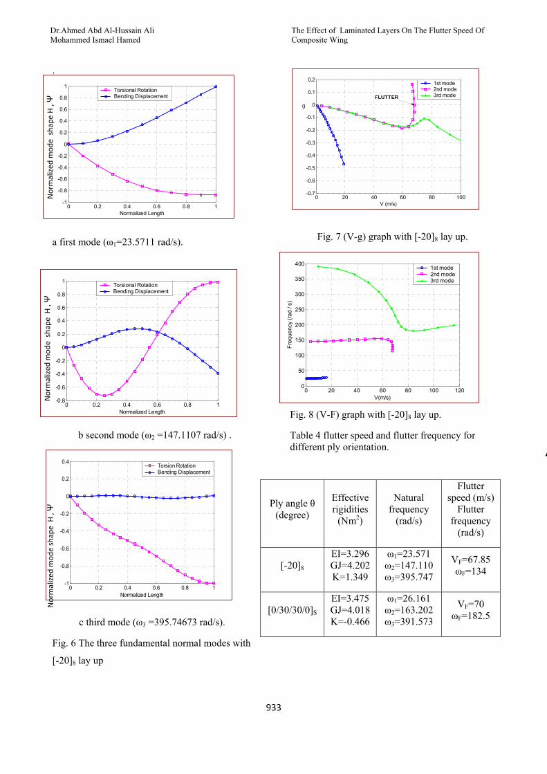
The Effect of Laminated Layers On The Flutter Speed Of Composite Wing
Dr.Ahmed Abd Al-Hussain Ali Mohammed Ismael Hamed
933
0 0.2 0.4 0.6 0.8 1-1
-0.8
-0.6
-0.4
-0.2
0
0.2
0.4
0.6
0.8
1
Normalized Length
Torsional RotationBending Displacement
Normalized
mod
e shape
H , Ψ
0 0.2 0.4 0.6 0.8 1-0.8
-0.6
-0.4
-0.2
0
0.2
0.4
0.6
0.8
1
Normalized Length
Torsional RotationBending Displacement
0 0.2 0.4 0.6 0.8 1-1
-0.8
-0.6
-0.4
-0.2
0
0.2
0.4
Normalized Length
Torsion RotationBending Displacement
0 20 40 60 80 100-0.7
-0.6
-0.5
-0.4
-0.3
-0.2
-0.1
0
0.1
0.2
V (m/s)
g
1st mode2nd mode3rd modeFLUTTER
0 20 40 60 80 100 1200
50
100
150
200
250
300
350
400
V(m/s)
Freq
uenc
y (ra
d / s
)
1st mode2nd mode3rd mode
.
a first mode (ω1=23.5711 rad/s).
b second mode (ω2 =147.1107 rad/s) .
c third mode (ω3 =395.74673 rad/s).
Fig. 6 The three fundamental normal modes with
[-20]8 lay up
Fig. 7 (V-g) graph with [-20]8 lay up.
Fig. 8 (V-F) graph with [-20]8 lay up.
Table 4 flutter speed and flutter frequency for different ply orientation.
Ply angle θ (degree)
Effective rigidities
(Nm2)
Natural frequency
(rad/s)
Flutter speed (m/s)
Flutter frequency
(rad/s)
[-20]8 EI=3.296 GJ=4.202 K=1.349
ω1=23.571 ω2=147.110 ω3=395.747
VF=67.85 ωF=134
[0/30/30/0]S EI=3.475 GJ=4.018 K=-0.466
ω1=26.161 ω2=163.202 ω3=391.573
VF=70 ωF=182.5
Normalized
mod
e shape
H , Ψ
Normalized
mod
e shape H , Ψ

Journal of Engineering Volume 18 August 2012 Number 8
934
Table 4 flutter speed and flutter frequency for different ply orientation.
Table 5 the comparison between the theoretical and experimental flutter speed and the relative error.
Volt(v)
Time(sec)
9a Bending response
Volt(v)
Time(sec)
9b Torsion response
Fig. 9 Bending and torsion response when (V=55.15m/s).
[45/0/45/0]S
EI=2.785 GJ=5.748
K=0
ω1=23.516 ω2=147.059 ω3=409.903
VF=87 ωF=186.65
[0/45/0/45]S EI=3.463 GJ=4.094
K=0
ω1=26.215 ω2=163.646 ω3=395.571
VF=71 ωF=183.57
[-25]8 EI=2.983 GJ=4.948 K=1.427
ω1=22.368 ω2=139.729 ω3=387.316
VF=72.742 ωF=125.07
[45/-45/45/-45]S
EI=2.070 GJ=7.127
K=0
ω1=20.278 ω2=126.923 ω3=354.617
VF=99 ωF=197
[45/30/45/-45]S
EI=2.255 GJ=6.772 K=-0.420
ω1=21.086 ω2=131.941 ω3=368.516
VF=99.286 ωF=192.55
[45/-45/45/-30]S
EI=2.080 GJ=7.109 K=0.022
ω1=20.324 ω2=127.212 ω3=355.416
VF=98.88 ωF=195.83
[45/-45/45/30]S
EI=2.080 GJ=7.109 K=-0.022
ω1=20.329 ω2=127.240 ω3=355.496
VF=101.88 ωF=195.13
Ply orientation
VF(m/s) theoretical
VF(m/s) experimental Error
[-20]8 67.85 55.15 18.7%

Journal of Engineering Volume 18 August 2012 Number 8
935
Study the Effect of Ceramic Coating on the Performance and Emissions of Diesel Engine
Dr. Ibtihal Al-Namie Dr. Mahmoud A. Mashkour
Ahmed Sabah Hameed
Abstract In this study, the effect of ceramic coating on the performance and gases emission on diesel engine was investigated. A four-stroke, direct injected, single cylinder, diesel engine was tested at constant speed and at different load conditions without coating. Then, the inlet and exhaust valves faces were coated by about 500µm with ceramic materials. Ceramic layers were made of Yttria-Stabilized Zirconia (YSZ), and NiCrAl as a bond coat. The coating technique adapted in this work is the flame spray method. The engine with valves ceramic-coated research was tested for the same operation conditions of the engine (without coating). The results indicate a reduction in both fuel consumption by about 7.6% and particulate emissions by about (13% for HC and 14.5% for CO) with increasing in exhaust gases temperature after coating. Keywords: Diesel engine, Ceramic coating, Engine performance, Exhaust emissions.
دراسة تأثير الطالء السيراميكي على أداء وانبعاثات محرك ديزل
الخالصةمحرك ديزل ل اتانبعاث الغاز دراسة تأثير الطالء الخزفي على أداء و تم، في هذا البحث
تم دراسة األداء لهذا المحرك بسرعة ثابتـة . حقن مباشر وأحادي االسطوانة األشواط ذو رباعي
مايكرون بمواد ) 500 (تم طالء وجه صمامي العادم والدخول بسمك .وحمل متغير قبل الطالء
مـسحوق طـالء حيث تم استخدام الزركونيا المثبتة بالياتيريا كماده طالء باالضافه الى .خزفية
اعتمدت تكنولوجيا الطالء الحـراري بتقنيـه ، في هذا العمل . األلمنيوم -كروم—رابط من نيكل
المحرك تحت نفس ظروف التشغيل قبل وبعد الطالء وقد أعطـت النتـائج اختبر . الرش باللهب
ان والنقـص 7.6%وبنسبة تحسين في اداء المحرك من ناحية النقصان في معدل استهالك الوقود
لغـاز احـادي اوكـسيد 4.5%للهيدروكربونات الغير محترقـة و 13%(في الملوثات وبنسب
.وزيادة في درجة حرارة غازات العادم بعد الطالء الكاربون
.غازات العادم، أداء المحرك، الطالء السيراميكي، محركات الديزل: مفاتيح الكلمات

Study the Effect of Ceramic Coating on the Performance and Emissions of Diesel Engine
Dr. Ibtihal Al-Namie Dr. Mahmoud A. Mashkour Ahmed Sabah Hameed
936
Nomenclature: BSFC- Brake specific fuel consumption (kg/ kW.h) CO2- Carbon dioxide CO- Carbon monoxide HC- Hydrocarbon (ppm) K- Thermal conductivity (W/m K) LHR- Low heat rejection N- Rotational speed (rpm) NOx- Nitrogen Oxides PSC- Plasma spray coating PSZ- Partially stabilized zirconia SN- Silicon Nitride SFC- Specific fuel consumption T- Exhaust gas temperature (°C) Tb- Torque of engine (N.m) TBC- Thermal barrier coating Wb- Brake power (kW) YSZ- Yttria-stabilized zirconia 1. Introduction and background
The automobile industry is facing a serious challenge to improve vehicle fuel efficiency. Global demand for cars is soaring - one forecast has the number of worldwide cars increasing five-fold by 2050 to 2.9 billion (Special report, 2008). In the scenario of increase of vehicle population at an alarming rate due to advancement of civilization, use of diesel fuel in not only transport sector but also in agriculture sector is leading to fast depletion of diesel fuels and increase of pollution levels with these fuels, efficient fuel utilization has become pertinent for the engine manufacturers, users and researchers involved in the combustion research. While search for alternate fuels is
continuing, researchers are also attempting to find different techniques of efficient fuel utilized in diesel engines (Murthy, 2010). Reductions in fuel consumption can be achieved by a variety of measures, including improved aerodynamics, weight reductions and hybrid power trains. Significant improvements must also be made to the efficiency of the internal combustion (IC) engine that powers nearly all the world's vehicles. One promising technology for improving IC engine efficiency, as well as performance and durability, is the Thermal Barrier Coating (TBC) (Murthy, 2010). TBC are duplex systems, consisting of a ceramic topcoat and a metallic intermediate bond coat. The topcoat consists of ceramic material whose function is to reduce the temperature of the underlying, less heat resistant metal part. The bond coat is designed to protect the metallic substrate from oxidation and corrosion and promote the ceramic topcoat adherence (İlker, 2010). A thermal barrier application is shown in fig. 1.
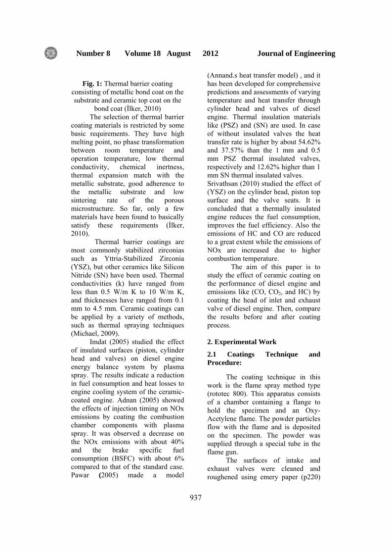
Journal of Engineering Volume 18 August 2012 Number 8
937
Fig. 1: Thermal barrier coating
consisting of metallic bond coat on the substrate and ceramic top coat on the
bond coat (İlker, 2010) The selection of thermal barrier
coating materials is restricted by some basic requirements. They have high melting point, no phase transformation between room temperature and operation temperature, low thermal conductivity, chemical inertness, thermal expansion match with the metallic substrate, good adherence to the metallic substrate and low sintering rate of the porous microstructure. So far, only a few materials have been found to basically satisfy these requirements (İlker, 2010).
Thermal barrier coatings are most commonly stabilized zirconias such as Yttria-Stabilized Zirconia (YSZ), but other ceramics like Silicon Nitride (SN) have been used. Thermal conductivities (k) have ranged from less than 0.5 W/m K to 10 W/m K, and thicknesses have ranged from 0.1 mm to 4.5 mm. Ceramic coatings can be applied by a variety of methods, such as thermal spraying techniques (Michael, 2009).
Imdat (2005) studied the effect of insulated surfaces (piston, cylinder head and valves) on diesel engine energy balance system by plasma spray. The results indicate a reduction in fuel consumption and heat losses to engine cooling system of the ceramic-coated engine. Adnan (2005) showed the effects of injection timing on NOx emissions by coating the combustion chamber components with plasma spray. It was observed a decrease on the NOx emissions with about 40% and the brake specific fuel consumption (BSFC) with about 6% compared to that of the standard case. Pawar (2005) made a model
(Annand.s heat transfer model) , and it has been developed for comprehensive predictions and assessments of varying temperature and heat transfer through cylinder head and valves of diesel engine. Thermal insulation materials like (PSZ) and (SN) are used. In case of without insulated valves the heat transfer rate is higher by about 54.62% and 37.57% than the 1 mm and 0.5 mm PSZ thermal insulated valves, respectively and 12.62% higher than 1 mm SN thermal insulated valves. Srivathsan (2010) studied the effect of (YSZ) on the cylinder head, piston top surface and the valve seats. It is concluded that a thermally insulated engine reduces the fuel consumption, improves the fuel efficiency. Also the emissions of HC and CO are reduced to a great extent while the emissions of NOx are increased due to higher combustion temperature.
The aim of this paper is to study the effect of ceramic coating on the performance of diesel engine and emissions like (CO, CO2, and HC) by coating the head of inlet and exhaust valve of diesel engine. Then, compare the results before and after coating process. 2. Experimental Work
2.1 Coatings Technique and Procedure: The coating technique in this work is the flame spray method type (rototec 800). This apparatus consists of a chamber containing a flange to hold the specimen and an Oxy-Acetylene flame. The powder particles flow with the flame and is deposited on the specimen. The powder was supplied through a special tube in the flame gun. The surfaces of intake and exhaust valves were cleaned and roughened using emery paper (p220)
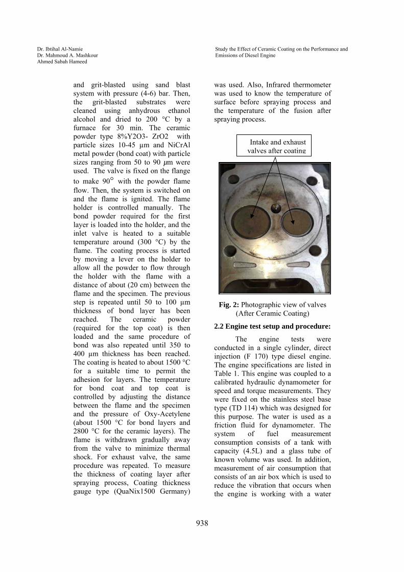
Study the Effect of Ceramic Coating on the Performance and Emissions of Diesel Engine
Dr. Ibtihal Al-Namie Dr. Mahmoud A. Mashkour Ahmed Sabah Hameed
938
and grit-blasted using sand blast system with pressure (4-6) bar. Then, the grit-blasted substrates were cleaned using anhydrous ethanol alcohol and dried to 200 °C by a furnace for 30 min. The ceramic powder type 8%Y2O3- ZrO2 with particle sizes 10-45 µm and NiCrAl metal powder (bond coat) with particle sizes ranging from 50 to 90 µm were used. The valve is fixed on the flange to make 90° with the powder flame flow. Then, the system is switched on and the flame is ignited. The flame holder is controlled manually. The bond powder required for the first layer is loaded into the holder, and the inlet valve is heated to a suitable temperature around (300 °C) by the flame. The coating process is started by moving a lever on the holder to allow all the powder to flow through the holder with the flame with a distance of about (20 cm) between the flame and the specimen. The previous step is repeated until 50 to 100 µm thickness of bond layer has been reached. The ceramic powder (required for the top coat) is then loaded and the same procedure of bond was also repeated until 350 to 400 µm thickness has been reached. The coating is heated to about 1500 °C for a suitable time to permit the adhesion for layers. The temperature for bond coat and top coat is controlled by adjusting the distance between the flame and the specimen and the pressure of Oxy-Acetylene (about 1500 °C for bond layers and 2800 °C for the ceramic layers). The flame is withdrawn gradually away from the valve to minimize thermal shock. For exhaust valve, the same procedure was repeated. To measure the thickness of coating layer after spraying process, Coating thickness gauge type (QuaNix1500 Germany)
was used. Also, Infrared thermometer was used to know the temperature of surface before spraying process and the temperature of the fusion after spraying process.
Fig. 2: Photographic view of valves
(After Ceramic Coating)
2.2 Engine test setup and procedure:
The engine tests were conducted in a single cylinder, direct injection (F 170) type diesel engine. The engine specifications are listed in Table 1. This engine was coupled to a calibrated hydraulic dynamometer for speed and torque measurements. They were fixed on the stainless steel base type (TD 114) which was designed for this purpose. The water is used as a friction fluid for dynamometer. The system of fuel measurement consumption consists of a tank with capacity (4.5L) and a glass tube of known volume was used. In addition, measurement of air consumption that consists of an air box which is used to reduce the vibration that occurs when the engine is working with a water
Intake and exhaust valves after coating
Journal of Engineering Volume 18 August 2012 Number 8
939
manometer. The temperature of exhaust gas was measured by a calibrated thermocouple (type K) that is fixed at the entrance of exhaust gas pipe (the beginning of the exhaust gas exit). The exhaust gas analyzer type (mod 488) was used to analyze gases the emissions of exhaust gases. It detects the CO-CO2-HC contents. The gases are picked up from the engine exhaust pipe by means of the probe. They are separated from the water they contain through the condensate filter and then they are conveyed to the measuring cell. A ray of infrared light, which is generated by transmitter, is sent through the optical filters on to the measured elements. The gases which contain the measuring cell absorb the ray of light at different wavelength, according to their concentration.
The engine was allowed to run with neat diesel fuel at a constant speed for nearly 10 min to attain the steady-state condition at the lowest possible load. The performance of engine was observed at a constant speed of 3000 rpm and varying load.
Table 1: Main technical specification
of engine
Technical Specification Item
170F Model Single-cylinder, vertical,4-stroke, air-cooled, direct-injection
Type
70 × 55 Bore×Stroke (mm) 0.211 Displacement (L) 2.5 Fuel tank capacity (L)
0.75 Full
0.25 Effective
Lubrication oil capacity (L)
Forced air cooled system Cooling type
Pressure, splash Lubrication type
Recoil manual start and optional electric start
Starting type
3. Mathematical Relationships Used to Calculate Engine Performance: (Ganesan, 2008; Mohanty, 2007)
1. Fuel consumption:
fuelf
f
.
timeV
m ρ∗= (1) Where: Vf - Volume of fuel consumption
fuelρ = 850 kg/m³ (As the specification of diesel oil from ALDORA refinery). 2. Brake Power:
( )kW000,60NT2
W bb
π=& (2)
Where: Tb - torque of engine (N.m) N- rotational speed (rpm) 3. Brake Specific Fuel Consumption:
⎟⎠⎞
⎜⎝⎛=
hr.kWkg3600*
Wm
BSFCb
f
&
& (3)
4. Results and discussion : Fuel consumption and exhaust temperature: A comparison of the BSFC for the standard engine (SE) and the ceramic coated engine (CE) under constant speed and varying load is shown in Fig. (3). Because of the

Study the Effect of Ceramic Coating on the Performance and Emissions of Diesel Engine
Dr. Ibtihal Al-Namie Dr. Mahmoud A. Mashkour Ahmed Sabah Hameed
940
higher surface temperatures of valves, the BSFC values of the LHR engine were lower than those of the standard engine. The relative reduction in the BSFC is seen to be within the range of 7.6%. Zirconia has a low thermal conductivity material. It will act as barrier for the heat transfer to the surroundings from the components engine’s combustion chamber and reduces the heat loss from the engine. Also, according to the first law of thermodynamics, the heat reduction in heat loss will ultimately increase the power output and thermal efficiency of the engine and this lead to reduce the BSFC.
Fig. 3: BSFC versus brake power, before and after ceramic coating, at constant speed engine
(3000 rpm) In Fig. 4, the exhaust gas temperatures from the two engine configurations are plotted as a function of load. It can be seen from the graph the temperature of the exhaust gas is higher for the engine works under zirconia coated conditions than the engine works under normal conditions. This is due to the more amount of heat generated inside the combustion chamber, where all amount of heat cannot be converted into useful work. Exhaust gas temperature increase under this condition because of this
heat that is mixed with the exhaust gas. The exhaust gas temperatures were seen to increase by 34.5 °C (on average) with the addition of insulation.
Fig.4: Exhaust gas temperature versus brake power, before and after ceramic
coating, at constant speed engine (3000 rpm)
Emissions: From the fig. 5, it is clear that the CO emission is less in LHR engine this may be due to the complete combustion. The carbon monoxide, which arises mainly due to incomplete combustion, is a measure of combustion in efficiency. Generally, oxygen availability in diesel is high so at high temperatures carbon easily combines with oxygen and reduces the CO emission. It is observed that at part load (up to 0.62 kW) the CO emissions are roughly same for the engine with and without coating. And there is an increase of CO at full load condition when it runs without coating conditions because of the specific fuel consumption increase.

Journal of Engineering Volume 18 August 2012 Number 8
941
Fig. 5: CO emission versus brake power,
before and after ceramic coating, at constant speed engine (3000 rpm)
The unburned HC emissions are higher when the engine works without the zirconia coating. The emission of unburned hydrocarbon from the LHR engines is more likely to be reduced because of the decreased quenching distance and the increased lean flammability limit. The higher temperatures both in the gases and at the combustion chamber walls of the LHR engine assist in permitting the oxidation reactions to proceed close to completion. In case of LHR engine with valves coating, HC is lower by about 13% than standard engine as shown in fig. 6.
Fig. 6: HC emission versus brake power, before and after ceramic coating, at constant speed engine
(3000 rpm)
5. Conclusion From the observations and test results reported herein, applying thin ceramic coatings of (0.5) µm to the intake and exhaust valves of diesel fuel combustion engine may result in a significant reduction in fuel consumption, and it causes the cylinder walls to become hotter and increases exhaust gas energy. Almost an average of 34.5 °C increase in the combustion gas temperature has been observed for the LHR engine compared to the standard engine. The brake specific fuel consumption (BSFC) values of the LHR engine were found to be lowered by about 7.6% than those of the standard engine because some of the additional heat energy in the cylinder is converted into useful work due to the insulation of the ceramic coating. The emission characteristics of the insulated engine at moderate and full loads appeared to be attractive. Particulate emissions decreased clearly in the LHR engine. These reductions were up to 13.2% for HC and 14.5% for CO. References Adnan P., Halit Y. , Can H. ,and Ahmet K."The effects of injection timing on NOx emissions of a low heat rejection indirect diesel injection engine " Applied Thermal Engineering, Elsevier, pp.3042 – 3052, 2005 . Ganesan, V., "Internal Combustion Engines", 3rd Edition, 2008. Imdat T., "An experimental study of energy balance in low heat rejection diesel engine”, Faculty of Engineering, University of Sakarya, Published by Elsevier Ltd, 2005.
Study the Effect of Ceramic Coating on the Performance and Emissions of Diesel Engine
Dr. Ibtihal Al-Namie Dr. Mahmoud A. Mashkour Ahmed Sabah Hameed
942
İlker T. Y., Metin G., and Mehmet A., "Thermal barrier coating for diesel engines ", International scientific conference, Gabrovo, November, 2010. Michael A. M., "An investigation of metal and ceramic thermal barrier coatings in a spark-ignition engine", Graduate Department of Mechanical and Industrial Engineering, Msc. thesis, University of Toronto., 2009. Mohanty R. K., "Internal Combustion Engines", McGraw-Hill, 2007. Murthy P.V. K, Murali K. M. V. S., Sitarama R. A. , Vara P. C. M ., and Srinivasulu N.V., "Performance Evaluation of Low Heat Rejection Diesel Engine with Pure diesel ", international journal of applied engineering research, dindigul Volume1, No 3, 2010.
Pawar A. N. , and Jajoo B. N. "Analysis of Heat Transfer in Ceramic Coated Cylinder Head and Valves of Diesel Engines", IE (I) Journal.MC, Vol 86, April 2005. Special Report: The art of the possible. Economist, http://www. economist.com/node/12544947, 2008. Srivathsan, P.R. Babu, P.T. Banugopan, V.N. Prabhakar, S. Annamalai, K. “Experimental Investigation on a Low Heat Rejection Engine", published by IEEE, 2010

Journal of Engineering Volume 18 August 2012 Number 8
961
Buckling Analysis Of Damaged Composite Plates Under Uniform Or Non-Uniform Compressive Load
Abstract.
The present study focused mainly on the buckling behavior of composite laminated plates subjected to mechanical loads. Mechanical loads are analyzed by experimental analysis, analytical analysis (for laminates without cutouts) and numerical analysis by finite element method (for laminates with and without cutouts) for different type of loads which could be uniform or non-uniform, uniaxial or biaxial. In addition to many design parameters of the laminates such as aspect ratio, thickness ratio, and lamination angle or the parameters of the cutout such as shape, size, position, direction, and radii rounding) which are changed to study their effects on the buckling characteristics with various boundary conditions. Levy method of classical laminated plate theory and Finite element coded by ANSYS 13.0 is used to formulate the theoretical model. Results are compared with other researches and good agreement was obtained.
Key words:
Composite, Buckling analysis, Finite element method, ANSYS program, uniform load, non-uniform load
الخالصة:
االحمال الميكانيكية . رضة الحمال ميكانيكيةعهذا البحث يرآز بصورة رئيسية على تصرف االنبعاج للصفائح المرآبة الم و طرق عددية بأستخدام طريقة العناصر المحددة) غير الحاوية على ثقوبللصفائح( تحليلية،تحليلها بطرق عملية تم
ألنواع مختلفة من األحمال التي من الممكن ان تكون منتظمة او غير )للصفئح التي تحتوي والتي ال تحتوي على ثقوب(سمكها و ، لصفيحة آالنسبة بين اطوالهاد آبير من عناصر التصميم لالى عد باألضافة باتجاه واحد او باتجاهين، منتطمة
يرها لدراسة يوالتي تم تغاالتجاه و نصف قطر الحافات ، الموقع، الحجم، زاوية ميالن الفايبر او متغيرات الثقوب آالشكلاستخدمت لتمثل ناصر المحددة نظرية الصفائح المرآبة التقليدية والع. تأثيرها على حمل االنبعاج مع اشكال اسناد مختلفة
. النموذج التحليلي وتمت مقارنة النتائج مع بحوث سابقة والحصول على توافق جيد بينها
Kawther Khalid Younus Mechanics Engineening Department
university of Baghdadmail: [email protected]
Prof. Dr. Adnan Naji Jameel Mechanics Engineening
Department university of Baghdad e-mail:[email protected]

Buckling Analysis Of Damaged Composite Plates Under Uniform Or Non-Uniform Compressive Load
Prof. Dr. Adnan Naji Jameel Kawther Khalid Younus
ج
962
Introduction
Laminated composites are gaining wider use because of their case of handling, good mechanical properties and low fabrication cost. They also possess excellent damage tolerance and impact resistance, excellent stiffness and weight characteristics. Cutouts are commonly found as access ports for mechanical and electrical systems or simply to reduce weight. The ability to monitor such
structures and detect damage before it reaches critical levels is of outmost importance in the composite material used in different fields, such plates which contain damages are vulnerable to buckle when subjected to various types of in-plane loadings; therefore it is of great importance to fully understand the effects of various parameters on its buckling load. Many researchers investigated this problem over the years from different perspectives; the following paragraphs summarize their works.
[Austin C. D. 2003] investigated the buckling of fiberglass reinforced plastic FRP laminated plates using the commercially available ANSYS finite element software. [1] [Ko.William L. 1998] studied the compressive buckling analysis on metal-matrix composite (MMC) plates (square, rectangle) with central square holes [2]. [Ko. William L. 1998] in this study mechanical- and thermal-buckling analyses were performed on rectangular plates (titanium alloy) with central cutouts [3]. [Kitsuda K. 1935] investigated experimentally the ultimate strength of rectangular steel plates under shearing stresses when the plate contains lightening holes, [4]. [Kumar A. R. 2009] examined experimentally the influence of cutout shape (circular, square and rectangular) on the buckling load of composite plate.[5]. [Lee Y. J. et.al 1989] studied the buckling behavior of orthotropic square plate, either with or without a central circular hole. Results showed that the existence of central circular holes may cause a higher buckling
strength than the plates without holes [6]. [Pradyumna
S. and Bandyopadhyay J. N.
2005] studied the buckling analysis of square composite plates with central circular cutout using a higher-order shear deformable plate element based on a higher-order theory. A simply supported edges conditions are considered. Results show that the buckling load decreases with the increase in cutouts size [7]. [Teh Hu H. and Lin B. 1995] studied the buckling resistance of symmetrically graphite/epoxy laminated plates (square, rectangle) and subjected to uniaxial compression [8]. [Tekin M. D. and Altan M. F.1996] investigated an approach buckling analysis to compare buckling load of the reinforced plate with circular hole and without hole [9]. [Therib J.H. 2004] this work includes performing mechanical buckling analysis on square and rectangular aluminum plates with central (square or circular) cutout compressed by a uniaxial load. [10].
From above literature review, it can be observed that all literatures are approximately limited to one type of load such as uniaxial uniform compressive buckling load, and one shape of cutout such as circle or square. i.e, there are no comparison between other shapes of cutouts or type of loads such as taking into consideration the non-uniform loads, enough types of boundary conditions or enough parameters which effect on the buckling behavior, In the present work, mechanical buckling analysis of laminated plates with elastic properties has investigated analytically, experimentally, and numerically. Under the present study, the formulations are based the classical laminated plate theory, buckling characteristics of SSSS, SCSC, SFSF, SFSC, SSSC, SSSF for cross-ply and angle-ply made up of fiber-glass composites are studied theoretically under uniaxial and biaxial compressive buckling load, In addition to the numerical analysis of the non-uniform compressive buckling load.
Theoretical analysis
The theoretical formulation is based upon the classical laminated plate theory (CLPT),

Journal of Engineering Volume 18 August 2012 Number 8
963
then equation of motion are derived and solved using Fourier series to obtain buckling by solving eigenvalue problem for different boundary conditions. Analytical solution for cross-ply and angle-ply laminated plate subjected to mechanical loads are obtained by using CLPT for Levy
solution.
Classical laminated plate theory
:Displacement
The classical laminated plate theory (CLPT) based on assuming the straight line perpendicular to the mid surface before deformation remains straight after deformation.
The displacement field of CLPT contains only three dependent variables [11]:
u(x,y)=(x,y)+z (x,y) (1. a)
v(x,y)=(x,y)+z (x,y) (1. b)
w(x,y)=(x,y) (1. c)
Where: , denote rotations about y and x-axes respectively, and , ,
denote the displacement components along (x, y, z) directions respectively of a point on the mid-plane (i.e…z=0).
:Stress and Strain
The total strains can be written as follows
= +z
=+z (2)
The transformed stress-strain relations of an orthotropic lamina in a plane state of
stress are; for , see [11] :
= (3)
The resultant of inplane force Nxx ,Nyy and Nxy and moments Mxx, Myy and Mxy acting on a laminate are obtained by integration of the stress in each layer or lamina through the laminate thickness. Knowing the stress in terms of the displacement, we can obtain the inplane force resultants Nxx, Nyy, Nxy, Mxx, Myy
and Mxy.
The inplane force resultants are defined as
=dz = dz
(4.a)
Where: , and are normal and shear stress.
=+
(4.b)
= z dz = z dz (5.a)
= +
(5.b)
Here, are the extensional stiffness, the coupling stiffness, and the bending
stiffness.
Buckling Analysis Of Damaged Composite Plates Under Uniform Or Non-Uniform Compressive Load
Prof. Dr. Adnan Naji Jameel Kawther Khalid Younus
ج
964
= ( - (6.a)
= ( - (6.b)
= ( - (6.c)
:Equation of motion
The Euler-lagrange equations are obtained by setting the coefficient of , ,
to zero separately [11] :
=0 (7.a)
: = 0 (7. b)
: + + +
+ =0 (7.c)
: Where - =
= -
, are compressive loads
These equations of motion (7 a-c) can be expressed in terms of displacements
), , by substituting the forces results from eqs. (4 , 5) into eq. (7.a) to (7.c) and get partial differential equations, then the analytical solution done by levy method as derived in [11].
Numerical analysis
:Element selection and modeling
An element called shell281 as shown in fig.(1) is selected which is suitable for analyzing thin to moderately thick shell structures. The element has eight nodes with six degrees of freedom at each node: translations in the x, y, and z axes, and rotations about the x, y, and z axes. It may be used for layered applications for modeling composite shells. It is include the
effects of transverse shear deformation. The accuracy in modeling composite shells is governed by the first order shear deformation theory. The shell section allows for layered shell definition, options are available for specifying the thickness, material, orientation through the thickness
of the layers [12].
Finite element method has been employed to analyze critical buckling load. The model was developed in ANSYS 13.0 using the 121 (11*11) quadrate elements. The global x coordinate is directed along the width of the plate, while the global y coordinate is directed along the length and the global z direction corresponds to the thickness direction and taken to be the outward normal of the plate surface. There are 11 elements in the axial direction and 11 along the width (i.e. 8424 DOF). Convergence study is the reasons for choosing the particular mesh used in this study. A linear buckling analysis (eigenvalue buckling) was performed on the model to calculate the minimum buckling load of the structure as in the following
equation:
([K] + [S])= {0}
Where: [K] = stiffness matrix [S] = stress matrix
= ith eigenvalue (used to multiply the loads which generated [S])
= ith eigenvector of displacements
Verification case studies
In the present study, Series of preselected cases are modeled to verify the accuracy of the method of analysis. The results are compared to analytical solution (Levy) and numerical solution (Finite element method).
*Comparison between analytical solution (levy method) and the FEM solution (ANSYS program) for the present work
Table (1): Dimensionless uniaxial buckling load)of SFSF anti-symmetric cross ply

Journal of Engineering Volume 18 August 2012 Number 8
965
laminates without cutout, h=1 (M.P. from table (4)
Table (2): Dimensionless uniaxial buckling load
% λ [FEM]
[7]
Present λ
[F.E.M]
d/b
5.64 5.25 5.5636 0.0 4.91 5.17 4.9163 0.1 3.27 4.65 4.4980 0.2
5.1 4.25 4.0352 0.3 0.05 3.83 3.8282 0.4
Symmetric cross-ply
a=b, b/h=100, SSSS, d=diameter of hole, b=plate
width, /=0.5 ,==,
=0.25
5.61 3.64 3.8564 0.5
From results above, it is obvious that the methods of solution gives better results for both analytical and numerical solution.
Experimental work of laminated composite plates
In the present work, two cases are studied, the first case study the buckling behavior on rectangular laminated composite plate without cutout, and the second case study the effect of cutout shape (circular, square) in square laminated plate on the buckling load.
Mechanical properties (Tensile test) and compressive behavior (buckling test) of (0/90/90/0) E-glass polyester laminated composite plates are calculated experimentally. Three purposes were planned to be investigated through this part. First: The manufactured models. Second: Evaluating the mechanical properties of cross-ply composite. Third: measuring the critical buckling load of the same composites.
Tensile test
Each laminate was oriented in longitudinal, transverse and angle relative to designated direction to determine the engineering parameters ,
, . Tensile test specimen include
standard geometry according to ASTM (D 638) and the mechanical properties for glass-polyester which obtained from tensile
test as shown in table (3) and table (4) for case1 and case 2 respectively.
Buckling test
In this study, for case1, buckling load of laminated plate determined analytically, numerically and experimentally. The laminated plate length was 220 mm, the width and thickness of it are 110 mm and 5.2 mm respectively as in fig.(3.a). For case2 buckling load of laminated perforated plate determined numerically and experimentally. Both laminated plates length=width was 125 mm and the thickness of it was 6 mm, and the area of each central cutout (circle, square) was 501.76 as in fig.(3.b.c). Simply supported boundary conditions were simulated along the top and bottom edges. The buckling load is determined from the load-displacement curve as shown in fig.(4)
Results of experimental work
(case1)
The buckling load for SFSF laminated plate was determined using analytical analysis, numerical analysis (F.E) and experimental analysis. The agreement between the three methods was generally good. The critical buckling load is shown in table (5).
It was obvious that the experimental buckling load is greater than analytical method and numerical method because either there may be bubbles or porosity in a part of specimen or it’s thickness is not uniform exactly or the fibers is not straight in a part or thickness of each layer is not constant.
(Discrepancy %)
Analytical (Levy)
FEM (ANSYS)
a/b
(0.57%) 3.4675 3.4875 0.5 (0.16%) 0.8541 0.8555 1 (0.026%) 0.3769 0.3768 1.5 (0.14%) 0.2109 0.2112 2

Buckling Analysis Of Damaged Composite Plates Under Uniform Or Non-Uniform Compressive Load
Prof. Dr. Adnan Naji Jameel Kawther Khalid Younus
ج
966
The analytical solution (Levy method) is nearest to experimental solution from numerical method (F.E) where the discrepancy between them is lower than numerical solution. It reaches to 7.49%.
(case2)
The buckling load for SFSF laminated square plate was determined using numerical analysis (F.E) and experimental analysis. The agreement between the two methods was generally good. The critical buckling load is shown in table (6).
It was obvious that the buckling load in the laminate with circular cutout is greater
than that with square cutout as expected and this result is similar to [5].
& nalytical Results and discussion of anumerical solutions
First part: analytical solution for laminates under uniaxial or biaxial compressive
buckling load
1. Uniaxial compressive buckling load as shown in fig (5):-
The non-dimensional buckling load =
1.1- Effect of aspect ratio:
Fig (6) show that in SSSF and SFSF the buckling load decrease when a/b increase with high percentage reaches to 72.2% and 75.4% in SSSF and SFSF respectively. On the other hand in SCSC the buckling load decrease with small percentage reaches to 3.6% when a/b varies from 0.5 to 1.5, Then, it′s increases when a/b varies from 1.5 to 2. The maximum buckling load in SCSC is at a/b=2. While the minimum is at a/b=1.5. It′s worth mentioning the buckling load in SCSC is higher than other cases because of B.C′S. effect.
1.2- Effect of boundary conditions for symmetric and anti-symmetric cross-ply.
From the results listed in table (7), it can be observed that the boundary conditions always effect on the buckling load, while changing the lamination from anti-symmetric to symmetric may increase the buckling load with small percentage reaches to 1.7% as in SSSC and SCSC, or decrease it as in SFSF and SFSC, or doesn't affect the buckling load as in SFSS and SSSS.
1.3-Effect of lamination angle:
It is shown from fig (7), the buckling load decrease and increase with different
percentage when varies from 10 to 80 . In both cases the buckling load decrease when varies from 10 to 45, then it's increase
when varies from 45 to 80. The maximum buckling load for both cases is at =10.
2. Biaxial compressive buckling load as shown in fig (8):-
The non-dimensional buckling load =
2.1-Effect of aspect ratio:
Fig (9) show the buckling load decrease with high percentage in SCSC and SSSC when a/b varies from 0.5 to 1 and increase when a/b varies from 1 to 2, this percentage reaches to 52.7% and 34.3% in SCSC and SSSC respectively. On the other hand in SSSS the buckling load decreases with high percentage when a/b increase reaches to 64%. It′s worth mentioning the buckling load in SCSC is higher than other cases, because of boundary conditions effects.
2.2- Effect of lamination angle:
It is shown from fig (10), the buckling load increase and decrease with different
percentage when varies from 10 to 80 . In all cases the buckling load increase when
varies from 10 to 45, then it's decrease when varies from 45 to 80. The maximum
buckling load for all cases is at =45.

Journal of Engineering Volume 18 August 2012 Number 8
967
2.3- Effect of boundary conditions for symmetric and anti-symmetric cross-ply
From the results listed in table (8), it can be observed that the boundary conditions always effect on the buckling load, while changing the lamination from anti-symmetric to symmetric may decrease the buckling load
Second part: numerical solution using ANSYS program for laminates damaged by
cutouts
3. Uniaxial uniform compressive buckling load with square cutout as shown in fig (11.a) and with the boundary conditions as shown in fig (11.b,c):-
The non-dimensional buckling load =
3.1- Effect of cutout shape:
From the results listed in table (9), it can be observed that inserting cutout to the plate always decrease the buckling load with high percentage, but changing the cutout shape could increase or decrease the buckling load with small percentage. The buckling load in SCSC is higher than other case because of B.C′S. effect. It′s worth mentioning the sequence of cutout shape from highest value of buckling load to smallest value isn′t a standard form, but it′s different for each type of boundary conditions or other effects.
For example in the case of square-hole, the load-carrying narrow side strips along the plate boundaries are practically under uniform compressive stress fields. For the circular-hole cases, the narrow compressed side strips are under stress concentration, which reduces the buckling strengths. This fact may explain why, for most of the cases studied the buckling strengths of the plates with square holes increase more at larger hole sizes than the plates with circular holes having the same area [3], this unusual buckling characteristics of circular and square cutouts similar to the results in [3].
3.2-Effect of cutout size:
Fig (12) shows the buckling load in SCSC decrease when c/b varies from o.1 to 0.2 then it's increase when c/b varies from 0.2 to 0.5 with percentage range (0.85% - 11.6%) and the maximum buckling load is at c/b=0. On the other hand, in SSSS the buckling loads decreases when c/b increase with percentage range (1.5% - 19%), this trend similar to [6]. It′s worth mentioning the buckling load in SCSC is higher than SSSS, because of B.C′S. effect.
3.3- Effect of radii rounding (radius of fillet):
Fig.(13) show in SCSC the buckling load decrease with percentage range (0.85% -5.9%) when (r) increase from 0 to 12.5. On the other hand, in SSSS the buckling load decrease and increase with percentage range (0.7% -2.7%) when (r) increase. The maximum buckling load in SSSS is at r=0. While the minimum buckling load is at r=10, this trend similar to [10].
3.4- Effect of aspect ratio:
Fig (14) shows the buckling load decrease with high percentage in SSSS when a/b varies from 0.5 to 1 reaches to 27.1%. Then, it′s increases when a/b varies from 1to 2 with small percentage when a/b varies from 1 to 1.5 reaches to 12.1% then this percentage gets higher when a/b varies from 1to 2. The maximum buckling load in SSSS is at a/b=2. While the minimum buckling load is at a/b=1. On the other hand, in SCSC the buckling load increase from high percentage 34.77% to small percentage 9.3912%, this case similar to [10]. It′s worth mentioning the buckling load in SCSC is higher than SSSS, because of B.C′S. effect.
3.5- Effect of length to thickness ratio (a/h):
In fig(15), it can be observed that the buckling load decrease with percentage reaches to 22.8% in SCSC and 8.8 in SSSS when a/h increase, but it was shown the opposite meaning because of the effect of

Buckling Analysis Of Damaged Composite Plates Under Uniform Or Non-Uniform Compressive Load
Prof. Dr. Adnan Naji Jameel Kawther Khalid Younus
ج
968
non-dimensional value on buckling load.
3.6- Effect of cutout position:
From the results listed in table (10), it can be observed that as the cutout move toward the center with the dimensions shown in fig(16) the buckling load increase in SCSC and decrease in SSSS. The buckling load in SCSC is higher than other case because of B.C′S. effect. The maximum buckling load in SSSS and the minimum buckling load in SCSC at e/a=f/b=0.250.
3.7-Effect of lamination angle:
It is shown from fig (17), the buckling load increase and decrease with different
percentage when varies from 10 to 80 . The buckling load in SCSC is higher than other case, but the percentage in SSSS is hugher than SCSCS where it′s reaches to 13.365%. The buckling load in SSSS
increase when change from 10 to 45 with percentage reaches to 26.31% and then
decrease when change from 45 to 80 with percentage reaches to 25.315%, the
maximum buckling load in SSSS is at =45, while the minimum buckling load is at =10. On the other hand, the buckling load increase and decrease with different percentage in SCSC reaches 10.8254% from
max.buckling load at =30 to min. at =80.
3.8-Effect of distance between cutouts center:
3.8. A- Distance between cutouts center parallel to the x-axis
Fig (18.a) shows that in both SCSC and SSSS the buckling load decrease when s/b varies from 0.2 to 0.3 then it′s increases when s/b varies from 0.3 to 0.5, the buckling load decrease and increase with percentage reaches to 4%. The maximum buckling load in both SCSC and SSSS is at s/b=0.5. While the minimum buckling load is at s/b=0.3.
3.8. b- Distance between cutouts center parallel to the y-axis
Fig (18.b) shows that in SCSC the buckling load decrease with percentage reaches to 3.8% when (s/a) increase, On the other hand in SSSS the buckling load increase when (s/a) increase.
3.8. c- Distance between cutouts center parallel to the diagonal
Fig (18.c) shows that in SCSC the buckling load decrease when s/b varies from 0.2 to 0.3 and increase when s/b varies from 0.3 to 0.5 with percentage reaches to 3%, On the other hand in SSSS the buckling load increase when s/b increases. The maximum buckling load in SCSC is at s/b=0.4, while the minimum buckling load is at s/b=0.3. It′s worth mentioning the buckling load in SCSC is higher than SSSS,
because of B.C′S. effect.
4. Uniaxial non-uniform compressive buckling load with fillet cutout as shown in fig (19.a) and with the boundary conditions as shown in fig (19.b,c):-
The non-dimensional buckling load =
4.1-Effect of cutout shape:
From the results listed in table (11), it can be observed that inserting cutout to the plate decrease the buckling load, and that the buckling load could be increase or decrease with changing the cutout shape in a sequence depends on the boundary conditions type. It′s worth mentioning in the case of SFSF that the buckling load varies with small percentage range (0.022% - 17.1%) it′s decrease with high percentage reaches to 43% when the plate having cutout in the shape of fuselage path′s window, On the other hand, in the case of SFSC the buckling load decrease with small percentage range (0.7% - 5.4%) but its decrease with high percentage reaches to 35.8% when the cutout change from square
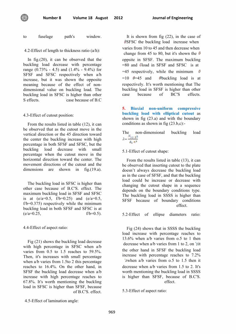
Journal of Engineering Volume 18 August 2012 Number 8
969
to fuselage path′s window.
4.2-Effect of length to thickness ratio (a/h):
In fig.(20), it can be observed that the buckling load decrease with percentage range (0.73% - 4.5) and (1.4% - 9.4%) for SFSF and SFSC respectively when a/h increase, but it was shown the opposite meaning because of the effect of non-dimensional value on buckling load. The buckling load in SFSC is higher than other
case because of B.CS effects.
4.3-Effect of cutout position:
From the results listed in table (12), it can be observed that as the cutout move in the vertical direction or the 45 direction toward the center the buckling increase with high percentage in both SFSF and SFSC, but the buckling load decrease with small percentage when the cutout move in the horizontal direction toward the center. The movement directions of the cutout and the dimensions are shown in fig.(19.a).
The buckling load in SFSC is higher than other case because of B.C′S. effect. The maximum buckling load in SFSF and SFSC is at (e/a=0.5, f/b=0.25) and (e/a=0.5, f/b=0.375) respectively while the minimum buckling load in both SFSF and SFSC is at (e/a=0.25, f/b=0.5).
4.4-Effect of aspect ratio:
Fig (21) shows the buckling load decrease with high percentage in SFSC when a/b varies from 0.5 to 1.5 reaches to 59.5%. Then, it′s increases with small percentage when a/b varies from 1.5to 2 this percentage reaches to 16.4%. On the other hand, in SFSF the buckling load decrease when a/b increase with high percentage reaches to 67.8%. It′s worth mentioning the buckling load in SFSC is higher than SFSF, because
of B.C′S. effect.
4.5-Effect of lamination angle:
It is shown from fig (22), in the case of SFSC the buckling load increase when
varies from 10 to 45 and then decrease when change from 45 to 80, but it's shown the oppsite in SFSF. The maximum buckling
load in SFSF and SFSC is at =80 and =45 respectively, while the minimum
buckling load is at=45 and =10 respectively. It′s worth mentioning that The buckling load in SFSF is higher than other case because of BC′S effects.
5. Biaxial non-uniform compressive buckling load with elliptical cutout as shown in fig (23.a) and with the boundary conditions as shown in fig (23.b,c):-
The non-dimensional buckling load =
5.1-Effect of cutout shape:
From the results listed in table (13), it can be observed that inserting cutout to the plate doesn’t always decrease the buckling load as in the case of SFSF, and that the buckling load could be increase or decrease with changing the cutout shape in a sequence depends on the boundary conditions type. The buckling load in SSSS is higher than SFSF because of boundary conditions
effect.
5.2-Effect of ellipse diameters ratio:
Fig (24) shows that in SSSS the buckling load increase with percentage reaches to 13.6% when a/b varies from o.5 to 1 then
it decrease when a/b varies from 1 to 2, on the other hand in SFSF the buckling load increase with percentage reaches to 7.2%
when a/b varies from o.5 to 1.5 then it decrease when a/b varies from 1.5 to 2. It′s worth mentioning the buckling load in SSSS is higher than SFSF, because of B.C′S.
effect.
5.3-Effect of aspect ratio:

Buckling Analysis Of Damaged Composite Plates Under Uniform Or Non-Uniform Compressive Load
Prof. Dr. Adnan Naji Jameel Kawther Khalid Younus
ج
970
Fig (25) show the buckling load decrease with high percentage reaches to 55% and 69% in SSSS and SFSF when a/b increase. It′s worth mentioning the buckling load in SSSS is higher than SFSF, because of B.C′S. effect.
5.4-Effect of cutout position:
From the results listed in table (14), it can be observed that in SSSS as the cutout move in the vertical direction or the diagonal direction toward the center the buckling load increase, but the buckling load increase then decrease when the cutout move in the horizontal direction toward the center. On the other hand, in SFSF the buckling load decrease as the cutout move in the diagonal direction toward the center, but the buckling load decrease then increase when the cutout move in the vertical or horizontal direction toward the center The movement directions of cutout and the dimensions are shown in fig(23.a). The buckling load in SSSS is higher than other case because of B.C′S. effect. The maximum buckling load in SSSS and the minimum in SFSF is at (e/a=0.5, f/b=0.25), while the minimum in SSSS and the maximum in SFSF is at (e/a=0.375,
f/b=0.5).
5.5-Effect of length to thickness ratio (a/h):
In fig.(26), it can be observed that the buckling load decrease with percentage range (1.8% - 9.7) and (0.8% - 5.4%) for SSSS and SFSF respectively when a/h increase, but it was shown the opposite meaning because of the effect of non-dimensional value on buckling load. The buckling load in SSSS is higher than other
case because of B.CS effects.
5.6-Effect of lamination angle:
It is shown from fig (27), in the case of SSSS the buckling load increase when
varies from 10 to 45 and then decrease when change from 45 to 80, but it's shown the oppsite in SFSF. The maximum buckling
load in SSSS and SFSF is at =45 and
=80 respectively, while the minimum buckling load is at=10 and =45
respectively. It′s worth mentioning that the buckling load in SSSS is higher than other case because of BC′S effects.
Conclusion
This study considers the buckling analysis of cross-ply and angle-ply damaged laminates with various B.C’S. From the present study, the following conclusions can
be made:
1. It was noted that inserting cutout to the plate doesn’t always decreases the buckling loads.
2. Changing the cutout shape (for the same cutout area) change the buckling load with small percentage (under 13%)
3. It was noted that when the cutout size increase, the buckling load doesn’t always decrease. The conventional wisdom is that, as the cutout size increase, the plates lose more materials and consequently lose more bending stiffness. The buckling loads are therefore expected to decrease as the cutout size increase, but sometimes and contrary to expectation, increasing the cutout size could increase the buckling load (anomalous buckling behavior) because of the strong boundary conditions (clamped rather than simply supported boundaries). i.e. losing more materials decrease the buckling load, but the strong boundary condition increase the buckling load. Thus, which effects become dominant will determine the increase or decrease of buckling load. The increase or decrease occurs with percentage range (0.9% - 21%).
4. When the cutout move toward the center in a direction parallel to the x-axis or y-axis or diagonal axis, in general the buckling load increase with percentage range (5% - 40%)
5. In general, as the aspect ratio increases, the critical buckling load of laminated plate decreases with high percentage

Journal of Engineering Volume 18 August 2012 Number 8
971
range (40% - 77%) in all types of compressive loads.
6. It was noted that different thickness ratio affected the critical buckling load. The buckling load decrease when a/h increase.
7. The buckling load decrease when the fiber angle varies from 10 to 45 and increase when the fiber angle varies from 45 to 80. On the other hand, the opposite behavior occurs in the cases of SSSS non-uniform biaxial compressive buckling load. In the case of undamaged laminate under biaxial compressive load, critical buckling load decreases when the fiber angle increase.
:References
[1] Austin C. D. "Buckling of symmetric laminated fiberglass reinforced plastic (FRP) plates". MSC. thesis, University of Pittsburgh; 2003.
[2].William L. "Anomalous buckling characteristics of laminated metal-matrix composite plates with central square holes". NASA TP 206559; 1998.
[3].William L. "Mechanical-and thermal-buckling behavior of rectangular plates with different central cutouts". NASA TM
206542;1998.
[4] Kitsuda K. "Investigation of stress distribution on thin metal sheet with holes ". Aeronautical engineer thesis, California
institute of technology; 1935.
[5] Kumar A.R. "Buckling analysis of woven epoxy laminated composite plate". MSC thesis, National institute of
technology; 2009.
[6] Lee Y.J., Lin H.J. and Lin C.C. "A study on the buckling behavior of an orthotropic square plate with a central circular hole" J composite structures 1989;13: 173-188.
[7] Pradumna S. and Bandyopadhyay J.N. "Static buckling analysis of laminated composite plates with a central circular
cutout using a higher-order element". J Int. J. of applied mechanics and engineering 2005; 11: 1-8. [8] Teh Hu H. and Lin B. "Buckling optimization of symmetrically laminated plates with various geometries and end conditions". J composite science and technology 1995;55:277-285.
[9] Tekin M. D. and Altan M. F. 1996 "The finite element analysis of buckling of laminated rectangular reinforced concrete plates with circular hole". J mathematical and computational applications 1996; 1(2):164-168. [10] Therib J.H. "An investigation of elastic buckling for perforated plates in aircraft structures" MSC. Thesis, AL-Rasheed college of engineering and science , university of technology; 2004.
[11] Reddy J.N. “Mechanics of laminated composite plates and shells: theory and analysis “. 2ed; CRC Press 2004.
[12] "Theory, analysis, and element manuals" ANSYS 13 Program.
Fig. 1 : Shell281 Geometry [12]
Table 3: Experimental unidirectional mechanical properties of fiber glass-
Polyester for case1:-
Mechanical properties
Glass-polyester
(Mpa) 25344 (Mpa) 4790.7 (Mpa) 2470
0.25
0.36
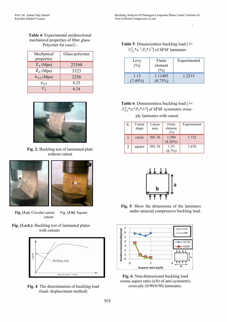
Buckling Analysis Of Damaged Composite Plates Under Uniform Or Non-Uniform Compressive Load
Prof. Dr. Adnan Naji Jameel Kawther Khalid Younus
ج
972
Table 4: Experimental unidirectional mechanical properties of fiber glass-
Polyester for case2:-
Mechanical properties
Glass-polyester
(Mpa) 23160 (Mpa) 3323 (Mpa) 2256
0.25
0.34
Fig. 2; Buckling test of laminated plate without cutout
Fig. (3.a): Circular cutout Fig. (3.b): Square cutout
Fig. (3.a.b.): Buckling test of laminated plates with cutouts
Fig. 4: The determination of buckling load (load- displacement method)
Table 5: Dimensionless buckling load [ = * / * ] of SFSF laminates
Levy (%)
Finite element
(%)
Experimental
1.13 (7.49%)
1.11485 (8.73%)
1.2215
Table 6: Dimensionless buckling load [ = * / * ] of SFSF symmetric cross-
ply laminates with cutout
S.
Cutout shape
Cutout area
Finite element
(%)
Experimental
1 circle 501.76 1.589 (8.26%)
1.732
2 square 501.76 1.53 (8.7%)
1.676
Fig. 5: Show the dimensions of the laminates under uniaxial compressive buckling load.
Fig. 6: Non-dimensional buckling load versus aspect ratio (a/b) of anti-symmetric
cross-ply (0/90/0/90) laminates.

Journal of Engineering Volume 18 August 2012 Number 8
973
Table 7: Dimensionless uniaxial buckling load of symmetric and anti-symmetric cross
ply laminates for different boundary conditions
Fig. 7: Non-dimensional buckling load versus lamination angle of anti-symmetric
angle-ply (θ/-θ/θ/-θ) laminates SFSF.
Fig. 8: show the dimensions of the laminates under biaxial compressive
buckling load.
Fig. 9: Non-dimensional buckling load versus aspect ratio (a/b) of anti-symmetric cross-ply
(0/90/0/90) laminates.
Fig. 10: Non-dimensional buckling load versus lamination angle of anti-symmetric
angle-ply (θ/-θ/θ/-θ) laminates.
(a) (b) (c)
Fig. 11: (a): show the dimensions of the laminates under uniform compressive buckling load (b), (c): show the boundary
conditions.
(0/90/90/0)
(0/90/0/90)
B.C'S
0.8392 0.8541 S-F-S-F 1.0053 1.0053 S-F-S-S 1.1374 1.1502 S-F-S-C 2.6603 2.6603 S-S-S-S 4.1044 4.0852 S-S-S-C
a=b=200, b/h=200
5.8999 5.1267 S-C-S-C

Buckling Analysis Of Damaged Composite Plates Under Uniform Or Non-Uniform Compressive Load
Prof. Dr. Adnan Naji Jameel Kawther Khalid Younus
ج
974
Table 8: Dimensionless uniaxial buckling load )of symmetric and anti-symmetric cross ply laminates for different boundary
conditions
Table 9: Non-dimensional uniaxial compressive buckling load with different type of boundary conditions for symmetric cross-ply laminates
(0/90/90/0).
Fig. 12: Buckling load versus cutout length to plate width ratio (a/b) of symmetric
cross-ply (0/90/90/0) laminates.
Fig. 13: Non-dimensional buckling load versus cutout radii rounding (r) of
symmetric cross-ply (0/90/90/0) laminates.
Fig. 14: Non-dimensional buckling load versus aspect ratio (a/b) of symmetric cross-ply
(0/90/90/0) laminates.
Fig. 15: Non-dimensional buckling load versus length to thickness ratio (a/h) of anti-symmetric angle-ply (30/-30/30/-30/30/-30)
laminates (thin and thick).
(0/90/90/0)
(0/90/0/90)
B.C'S
1.3312 1.330 S-S-S-S 1.8914 1.883 S-S-S-C
a=b=200, b/h=200
2.9329 2.907 S-C-S-C
a=150, b=140, h=6mm all cutouts of the same area=1225 SFSF SCSC SSSS
Cutout shape
Cutout shape
Cutout shape
S
0.7322 Without 5.3860 Without 2.3312 Without 10.5734 Diamond 4.8637 Square 1.5853 Square 20.5623 Ellipse 4.5288 Fillet 1.5515 Fillet 30.5509 Rectangle 4.4648 Rectangle 1.5252 Circle 40.5453 Fuselage
path’s windows
3.3547 Circle 1.5384 Rectangle 5
0.5140 Square 4.3253 Fuselage path’s
windows
1.5097 Fuselage path’s
windows
6
0.5092 Fillet 4.1358 Ellipse 1.4851 Ellipse 70.5034 Circle 4.1539 Diamond 1.4523 Diamond 8

Journal of Engineering Volume 18 August 2012 Number 8
975
Fig. 16: Show the dimension of the laminates under compressive buckling load.
Table 10: Non-dimensional uniform compressive buckling load of symmetric
cross-ply laminates (0/90/90/0) with square cutout
Fig. 17: Non-dimensional buckling load versus lamination angle of anti-symmetric
angle-ply (θ/-θ/θ/-θ) laminates.
Fig 18.a: Non-dimensional buckling load versus distance between cutout center to
plate width ratio (s/b) of symmetric cross-ply (0/90/90/0) laminates.
Fig. 18.b: Non-dimensional buckling load versus distance between cutout center to
plate width ratio (s/b) of symmetric cross-ply (0/90/90/0) laminates.
0123456
0 0.5 1
Non
dimen
sion
al buckling
load
s/b
SCSC
b/h=140a=150h=1mmc=24.7
Fig. 18.c: Non-dimensional buckling load versus distance between cutout center to
plate width ratio (s/b) of symmetric cross-ply (0/90/90/0) laminates.
( ),SCSC ( ), SSSS f/b e/a S
4.4456 2.1025 0.250 0.250 14.7934 1.8961 0.375 0.375 24.6319 1.9985 0.250 0.500 34.8393 1.8219 0.375 0.500 44.8597 2.0747 0.500 0.250 54.9183 1.8555 0.500 0.375 64.9966 1.7820 0.500 0.500 7
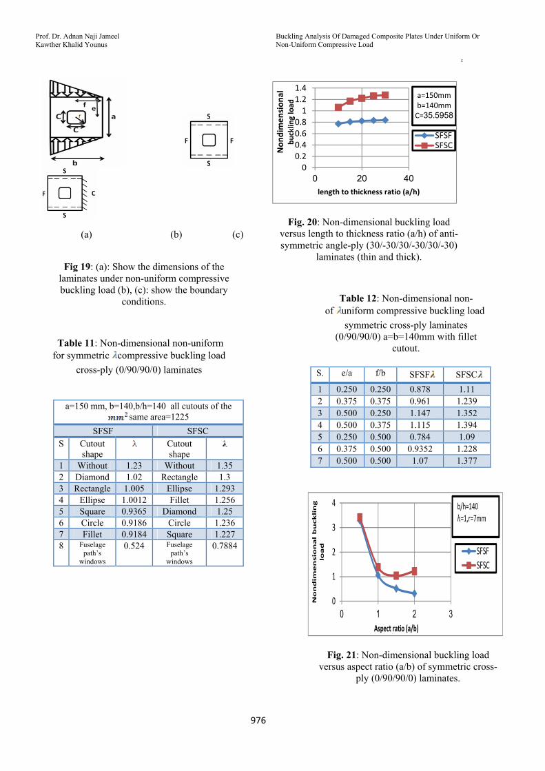
Buckling Analysis Of Damaged Composite Plates Under Uniform Or Non-Uniform Compressive Load
Prof. Dr. Adnan Naji Jameel Kawther Khalid Younus
ج
976
(a) (b) (c)
Fig 19: (a): Show the dimensions of the laminates under non-uniform compressive buckling load (b), (c): show the boundary
conditions.
Table 11: Non-dimensional non-uniform compressive buckling load for symmetric
cross-ply (0/90/90/0) laminates
00.20.40.60.81
1.21.4
0 20 40
Non
dimen
sion
al
bucklin
g load
length to thickness ratio (a/h)
SFSFSFSC
a=150mmb=140mmC=35.5958
Fig. 20: Non-dimensional buckling load versus length to thickness ratio (a/h) of anti-symmetric angle-ply (30/-30/30/-30/30/-30)
laminates (thin and thick).
Table 12: Non-dimensional non-uniform compressive buckling load of symmetric cross-ply laminates
(0/90/90/0) a=b=140mm with fillet cutout.
0
1
2
3
4
0 1 2 3
Nondim
ensional buckling
load
Aspect ratio (a/b)
SFSFSFSC
b/h=140=1,r=7mm
Fig. 21: Non-dimensional buckling load versus aspect ratio (a/b) of symmetric cross-
ply (0/90/90/0) laminates.
SFSC SFSF f/b e/a S.
1.11 0.878 0.250 0.250 1 1.239 0.961 0.375 0.375 2 1.352 1.147 0.250 0.500 3 1.394 1.115 0.375 0.500 4 1.09 0.784 0.500 0.250 5
1.228 0.9352 0.500 0.375 6 1.377 1.07 0.500 0.500 7
a=150 mm, b=140,b/h=140 all cutouts of the same area=1225
SFSC SFSF
Cutout shape
Cutout shape
S
1.35 Without 1.23 Without 1 1.3 Rectangle 1.02 Diamond 2
1.293 Ellipse 1.005 Rectangle 3 1.256 Fillet 1.0012 Ellipse 4 1.25 Diamond 0.9365 Square 5 1.236 Circle 0.9186 Circle 6 1.227 Square 0.9184 Fillet 7
0.7884 Fuselage path’s
windows
0.524 Fuselage path’s
windows
8

Journal of Engineering Volume 18 August 2012 Number 8
977
Table 13: Non-dimensional non-uniform compressive buckling load with different type
of boundary conditions for symmetric cross-ply (0/90/90/0) laminate
00.20.40.60.81
1.21.41.6
0 50 100
Non
dimen
sion
al buckling
load
lamination angle (θْ)
SFSFSFSC
a=150,b=140=140
C=35.5958r=7mm
Fig. 22: Non-dimensional buckling load versus lamination angle of anti-symmetric angle-ply
(θ/-θ/θ/-θ) laminates.
(a) (b) (c)
Fig. 23: (a): show the dimensions of the laminates under non-uniform compressive buckling load (b), (c): show the boundary
conditions.
Fig. 24: Non-dimensional buckling load versus ellipse diameters ratio / of symmetric cross-
ply (0/90/90/0) laminates.
a=150mm, b=140,b/h=140 all cutouts of the same area=1225
SFSF SSSS
Cutout shape Cutout shape
S
0.932 Ellipse 2.06 Without 1 0.924 Fillet 1.8155 Diamond 2
0.9052 Rectangle 1.71 Fillet 3 0.8951 Without 1.699 Circle 4 0.8947 Diamond 1.687 Ellipse 5 0.8876 Fuselage path’s
windows 1.66 Fuselage path’s
windows 6
0.8819 Circle 1.649 Square 7 0.8671 Square 1.5889 Rectangle 8

Buckling Analysis Of Damaged Composite Plates Under Uniform Or Non-Uniform Compressive Load
Prof. Dr. Adnan Naji Jameel Kawther Khalid Younus
ج
978
0
1
2
3
4
5
0 2 4Non
dimen
sion
al buckling load
Aspect ratio (a/b)
SSSSSFSF
b/h=140=1mm
Fig. 25: Non-dimensional buckling load versus aspect ratio (a/b) of symmetric cross-
ply (0/90/90/0) laminates.
Table 14: Non-dimensional non-uniform compressive buckling load of symmetric
cross-ply laminates (0/90/90/0) a=150, b=140mm with elliptical cutout.
SFSF SSSS f/b e/a S.
0.823 1.712 0.250 0.250 1 0.928 1.7 0.375 0.375 2 0.822 1.782 0.250 0.500 3 0.909 1.663 0.375 0.500 4
0.8752 1.6723 0.500 0.250 5 0.94 1.648 0.500 0.375 6 0.932 1.687 0.500 0.500 7
Fig. 26: Non-dimensional buckling load versus length to thickness ratio (a/h) of anti-symmetric angle-ply (30/-30/30/-30/30/-30) laminates (thin and thick).
Fig. 27: Non-dimensional buckling load versus lamination angle of anti-symmetric
angle-ply (θ/-θ/θ/-θ) laminates.

Journal of Engineering Volume 18 August 2012 Number 8
979
Application of Geographic Information System for Preparing the Bill of Quantities of Construction Projects
Ruqaya Hadi Rasheed
E-Mail:[email protected] Asst. Prof. Dr. Sedki Esmaeel Rezouki
Univercity of Baghdad Department of Civil Engineering E-Mail: [email protected]
Abstract The information required for construction quantities surveying is not only generated by various participants in different construction phases but also stored in different forms including graphics, text, tables, or various combinations of the three. To report a bill of quantities (BOQ), the project manager has to continuously excerpt information from various resources and record it on papers. Without adequate staff and time, this repetitive and tedious process is difficult for the project manager to handle properly and thus reduces the effectiveness and the accuracy of the quantities surveying process which creates problems during the design, tender, and construction supervision of construction projects for designers and contractors practicing because receipts are based upon actual quantities, such variations have an obvious impact on the contractor’s cash flow, once the actual quantities frequently vary from the estimated quantities listed in the BOQ. Hence, automation quantity surveying system has been developed by using GIS to extract the data required for the quantity of different components of any construction project from AutoCAD drawings (spatial data), to report a BOQ after querying, manipulation, and analyzing these data. The system has been implemented on the construction project of Al khawarizmy College at Baghdad University in Baghdad. The main results of using this system are automatic generation a bill of quantity (BOQ) directly from design drawing, with overcome to design changing, accurate, fast, and effective method for estimating the quantities, fewer errors in cost estimating, and better documentation for continuously reusing information in all construction phases. The accuracy of GIS quantities had been proved by comparing these quantities with the quantities of site surveying. Then determining the accuracy percentage (A%) of GIS quantities which equals (98.85%), and the regression line that equals 0.999. These values mean; there are big correlation between the estimated quantities by GIS and the quantities of site surveying. Keywords: GIS, BOQ.
أستخدام نظم المعلومات الجغرافية العداد جداول آميات المشاريع األنشائية قي اسماعيل رزوقيد صد.م.أ
قسم الهندسه المدنيه / جامعة بغداد رقية هادي رشيد
الخالصة
المطلوبة للمسح الكمي في المشاريع االنشائية تنتج من مختلف المشارآين في مراحل التشيد المختلفة و تكون ان المعلومات و .بعضهامحفوظة بصيغ مختلفة تتضمن الرسومات أو النصوص أو الجداول، أو قد تكون محفوظة بدمج هذه الصيغ الثالثة مع
روع ان يقتطف المعلومات بأستمرار من المصادر المختلفة و ان يقوم من مدير المش)BOQ( أعداد قائمة الكميات لذلك يتطلبوبدون وقت و عدد موظفين آافي سوف يكون من الصعب على مدير المشروع ان يدير عملية جمع . بتسجيلها على الورق
لى خلق المشاآل خالل المعلومات المتكررة و المملة بشكل صحيح ،و هذا يقلل من آفاءة و دقة عملية المسح الكمي مما يؤدي امرحلة التصميم و العطاء و االشراف خالل مرحلة التشيد للمصمم والمقاول بسبب ان االيصاالت المالية تعتمد على الكميات
عن الكميات المنفذة موقعيا ح على التدفق المالي للمقاول و ذلك الختالف الكميات ضالواقعية و أي اختالف يسبب تأثير والذلك قامت الباحثة بتطوير نظام اتمتة المسح الكمي باستخدام نظم المعلومات .)BOQ(مة الكمياتالمخمنة في قائ

Dr. Sedki Esmaeel Rezouki Application Of Geographic Information System For Ruqaya Hadi Rasheed Preparing The Bill Of Quantities Of Construction
Projects
980
اي مشروع انشائي من رسومات االوتوآاد فقراتوالذي يقوم باستخراج البيانات المطلوبة لكميات )GIS(الجغرافية)AutoCAD() (، ألعداد قائمة الكميات)البيانات المكانيةBOQ (صاء و معالجة و تحليل تلك البيانات بواسطة نظمبعد استق
و لقد طبق النظام على مشروع تشيد آلية الخوارزمي في جامعة بغداد في بغداد و تبلغ مساحة ) . GIS(المعلومات الجغرافية نتائجهم أ من ان. قاعة و مرافق اخرى لمختلف االغراض92 متر مربع، و تتكون الكلية من طابقين و 5508هذا المشروع
مباشرة من الرسومات التصميمية مع تغطية لجميع التغيرات التصميمية، و ) BOQ(استخدام هذا النظام هي انتاج قائمة الكميات بطريقة دقيقة و فعالة لتخمين الكميات، مما يؤدي الى اقل اخطاء في تخمين الكلف و انتاج وثائق يمكن استخدامها في جميع
من خالل مقارنتها مع قيم الكميات المنفذة فعليا في موقع )GIS(ثبتت دقة الكميات المخمنة بواسطة الو لقد ا. مراحل التشيداضافة الى ، % 98.85 والتي بلغت )GIS(وحساب النسبة المئوية لدقة آميات ال، عمل مشروع بناء هندسة الخوارزمي وهو قريب من واحد و هذا 0.999 (R²)قد بلغ هذا المعامل و الكميات المنفذة و)GIS(احتساب معامل االنحدار بين آميات ال
.يدل على ترابط آبير بين هذه القيم
جداول الكميات، المعلومات الجغرافية نظم: الكلمات الرئيسية 1. Introduction Progress in computerization and other automation techniques provides a great opportunity for improvement in construction materials management. Currently, the computer-aided design (CAD) system is widely used in engineering for drafting and design. As these CAD systems evolve, they are capable of generating materials requirements during the drawing phase and can be used to produce takeoff quantities. The benefit associated with this type of system is that a detailed takeoff of required quantities can be obtained directly from the CAD system, thereby eliminating the need to perform a detailed manual takeoff. However, because of the CAD system constraints of aggregating and distributing databases between locational and thematic attributes, the containing information, such as materials types, quantities, location demands, and need dates, within the system cannot be automatically extended and reused in the construction phase for material planning purposes. The geographic information system (GIS), which combines a CAD-like design program with a relational database management system for spatial data analysis, appears to have potential in solving these problems. By replacing CAD with GIS, the bill of quantities (BOM) is generated based on the dimensions of the design drawings, thus incorporating a linkage of locational and thematic information.
2. Research Objectives The main objective behind this paper was to develop an easy to use GIS based approach for quantity takeoffs in building construction. Other sub objectives that were to be achieved include accurate BOQ and development of construction resource database within GIS. 3.Gis In Construction Management GIS is an appropriate technology to fulfill various requirements of the construction projects. It is capable of integrating diverse data sets, databases, and various applications. GIS improves collective decision making among planners, designers, and contractors [Mohamed, Jeffrey, Guy, and Alan, 1993].Therefore, reported works suggest that GIS is supporting the construction industry in several areas such as [Bansal, 2007]: 1. Subsurface Profile, 2. Quantity Takeoffs and Construction Cost
Estimation, 3. Materials Layout at Construction Site, 4. Construction Site Layout, 5. Real -Time Schedule Monitoring
System, 6. Route-Planning and, 7. Topography Visualization 3. 1. Subsurface Profile [Camp and Brown,1993] suggested the use of GIS to develop a procedure for generating subsurface profiles from well-log data. The well-log database was constructed

Journal of Engineering Volume 18 August 2012 Number 8
981
from a series of borehole and GIS-base procedure was used to create 3D subsurface. [Oloufa and Papacostas, 1994] highlighted that site investigation is an important step in estimating and planning new construction projects and suggested the use GIS-based methodology to develop a database for foundations analysis, design and construction planning. As surface and subsurface conditions influence construction methods and choice of equipment, which in turn affect cost and scheduling of projects. Therefore, this study used database management capability of GIS to store descriptive soil data and to relate this data with the corresponding locations of boreholes.[ Joshphar, Ganeswara, and Kok-Kwang, 2005] developed the national geotechnical information system (GeoInfoSys) for Singapore by integrating GIS with a relational database management system (RDBMS) to develop a web-based geotechnical information system that can perform online spatial queries, generation of professional borelogs, and various geotechnical analysis. [Parsons, and Frost,2000] developed the GIS-ASSESS, which is a GIS-based tool designed to permit assessment of the adequacy, or thoroughness, of an investigation. GIS ASSESS was designed to be compatible with existing geostatistical software. It is capable of analyzing multidimensional data from multiple tools. 3.2. Quantity Takeoffs and Construction Cost Estimation
[Cheng and Yang,2001] suggested an approach for quantity takeoffs and cost estimation using Map/Info. Architectural drawing was divided into different layers, called data layers, for quantity takeoffs. In GIS-based cost estimates, area and perimeter were used as the basic parameters. Thus, data layers were created as polygons in AutoCAD and transferred to Map/Info in the form of geometric coverage. The geometric information of spatial features such as coordinate, area, perimeter and spatial relationship are derived from coverage.
Whereas, user enters thematic information such as identification (ID) code, beam number, floor number, etc. Recently, [Bansal and Pal, 2006] suggested the use of GIS for cost estimation in a more generalized way by adding new scripts into GIS environment for various cost estimation operations. ArcView, which utilizes the dynamic linkage between spatial and attribute data, was used for this purpose. 3. 3.Materials Layout at Construction Site
The MaterialPlan, a GIS-based tool developed by [Cheng and Yang, 2001] integrates quantity takeoffs with material layout planning. The system uses rules of thumb and experience to decide the size and location of material storage area. It assists planner in quantity takeoffs as well as in assessing material layout design. MaterialPlan developed by using a GIS environment integrate estimates with construction scheduling for dynamic materials requirement plan. Based on the information regarding quantities and locations of materials required in the project, the proposed methodology identifies the suitable site to store construction materials. 3.4. Construction Site Layout
The conventional approach to layout temporary facility (TFs) involves designing site layout using sketches, templates and 2D physical model. The developed layout is based upon the incomplete information stored in the different form. Such visual representations of TFs do not yield adequate and descriptive results. As TFs should be located close to their supporting activities to reduce the time for travel, the role of GIS may be explored for this. [Cheng and O’Connor, 1996] developed an automated site layout system called ArcSite using GIS for construction TFs. ArcSite consist of a GIS integrated with DBMS was claimed a new computerized tool to identify suitable area to locate TFs. ArcSite integrate information required to find suitable location for TFs and perform series of

Dr. Sedki Esmaeel Rezouki Application Of Geographic Information System For Ruqaya Hadi Rasheed Preparing The Bill Of Quantities Of Construction
Projects
982
complicated spatial operations and database queries to identify optimal site that is difficult to perform manually. ArcSite is a useful tool for construction site layout but the location of construction equipment as an important factor is not also considered in the system and the resulting layout of facilities may not arrive at the optimal solution. So that, [Sebt, Parvaresh, and Delavar, 2008] developed the system of GIS models which categorized into three parts; tower cranes, concrete batch plant, and temporary buildings. 3. 5. Real -Time Schedule Monitoring System The commercially available scheduling tools such as: Primavera and Microsoft Project fail to provide information pertaining to spatial aspects of a construction project. Therefore Bansal integrated 3D model developed in AutoCAD and construction schedule developed in Microsoft Excel. Spatial and scheduling information are linked together into a GIS environment. Linking an activity with its schedule involves adding a field called key to schedule and its attribute table. The field key is common between two tables and used to establish the connection between the spatial aspect of activity and the corresponding activity in the schedule. All the entries in the field key are to be entered manually and should be unique in both schedule and attribute tables of an activity[Bansal,2007]. Furthermore instead of Microsoft Excel, Stephen and David were generating construction schedule by Primavera Project Planner (P3) then linked with Spatial information into GIS [Stephen and David, 2006 ]. Bansal and Pal used ArcView GIS for generating bar charts using its in-built chart document. Figure (1) shows the ArcView’s chart document, utilized to show the schedule of the construction activities. The main advantage of the ArcView’s chart document over conventional bar chart is that when a bar on bar chart in ArcView is clicked, a window appears which provide the information
related to that particular activity [Bansaland Pal, 2006]. 3.6. Route-Planning
Planning access routes for construction site is an important consideration in the development of an effective project-execution plan. The constructability and the maintainability of an industrial facility can be impaired if the access routes are not considered during project planning [Construction Management Committee of the ASCE Construction Division. 1991]. Hence Varghese, and O’Connor used GIS for selection a suitable route from many alternative by analyzing a number of scenarios via creating site geometry using AutoCAD environment and create geometry of vehicle turn envelopes then convert it to Arc/Info coverages, establish spatial relationships between roads, turns, and potential obstacles, and run graphical queries to gather additional information on road attributes and conduct analysis [Varghese, and O’Connor, 1995]. 3. 7. Topography Visualization
GIS is an effective tool to visualize the topographical conditions of construction site. The modeling of construction site facilitates in construction controlling and planning process. GIS-based visual simulation system (GVSS) developed by Zhong and Song, is a tool that offers powerful planning, visualizing and querying capabilities as well as facilitate the detection of logical errors in a model [Zhong and Song, L., 2004]. 4. Proposed Approach For Gis- Based Quantity Surveying Automation quantity surveying by GIS is developed by using AutoCAD for producing spatial data (design drawings), and ArcGIS which have been used to extract, queried, manipulate, and analysis the quantity of different components of any construction project, from AutoCAD drawings, for reporting BOQ.

Journal of Engineering Volume 18 August 2012 Number 8
983
The proposed approach for automation BOQ by GIS can be categorized into: 1. Creating work breakdown structure 2. Creating AutoCAD drawings 3. Transferring AutoCAD drawings to
ArcMap 4. Converting AutoCAD drawings to GIS
format 5. Data integration 6. Creating database 7. Data manipulation and analysis. The proposed approach for GIS- based quantity surveying implemented on the finished activities of the Al Khwarizmy College building as a construction project, according to design specification and the Iraqi United Standard Guide of Quantity Surveying for Building Works and Civil Engineering to compare the quantities estimated by GIS with the quantities that obtained from site surveying. Al Khwarizmy project lies at Baghdad University at Al Jadyria section in Baghdad city. The area of the project is (5508 m²), the college consists of two floors with (92) rooms and other facilities for different purposes. The cost of the project is (ID 7.6 milliard). 4. 1. Creating Work Breakdown Structure
Work Breakdown Structure (WBS) illustrates the activities of the construction project according to the basic design of the project, to determine the data required for preparing BOQ, and to classify the layer of data for determining how many layers will represent the architectural design (AutoCAD drawings) that are required for preparing BOQ. 4. 2. Creating AutoCAD Drawings
AutoCAD drawings must be created to represent the data layer that required for any construction project. So, AutoCAD drawings have been created for the real life project that has been taken as a work field for this research are foundation, tie beams,
columns, beams, slaps, walls, stairs, parapets. 4. 3. Transferring AutoCAD Drawings to ArcMap
After creating drawings in AutoCAD, the dwg files were transferred to ArcMap a module of ArcGIS. The topologic data structure of the basic design layers in AutoCAD was created as layers in GIS based on the layers and activities identified in the AutoCAD drawings. 4. 4. Converting AutoCAD Drawings to GIS Format The basic parameters required for quantity takeoffs are area, perimeter and depth. Thus, the topologic data structure of the basic design (AutoCAD drawings) layers are created as polygons or polyline via ArcMap and ArcCatalog (Figure 2). 4. 5. Data Integration The geometric dimensions of the polygons or polyline in a single layer in some cases are insufficient for estimating the quantities of the activities, hence, join function of ArcMap is used to integrate layers. Thereby all the fields of the source attribute table are added to the destination table. 4. 6. Creating Database In addition to the database that has been created with the editing process which includes objected, shape, length, and area. There is a need for creating a database via GIS analysis tools, such as: total area, codes, total volume, and etc. 4.7. Data Manipulation and Analysis
After extracting the required data from AutoCAD drawings by creating a feature class for each drawing, these data have been manipulated and analyzed to estimate the quantities and report BOQ.

Dr. Sedki Esmaeel Rezouki Application Of Geographic Information System For Ruqaya Hadi Rasheed Preparing The Bill Of Quantities Of Construction
Projects
984
5. The Comparison between The Quantities Of Gis, Boq And Site Surveying
After creating the bill of quantity by GIS by benefiting from the ability of GIS for creating reports, a comparison has been made between the quantities of GIS, BOQ and site surveying. This comparison show that The difference between the quantities that estimated by GIS and that obtained by site surveying is small as illustrated in Table (1) and the accuracy percentage of GIS (A%) that equals (98.85%) as illustrated below. While there are a big difference between tender quantities and quantities of site surveying in some items, and that causes to inaccurate the conventional estimation method. However, the difference between the quantities of GIS estimation and site surveying can be to many causes such as; 1. The difference between the accuracy of
automated caused computer and human, especially when we know that there are more than one engineer has surveyed the quantities in the site and calculate the final values.
2. Depending on the payment of completed works on the quantity surveying for the finished activities in the site, hence the value of this quantity may be reduced if the contractor does not complete the activity according to the specification of the work.
3. Neglect the modification factor that must be run on the measurements of the surveying tools.
4. The difference between the drawing dimensions and the actual dimensions due to the variation orders in construction phase, or because to the difference between the accuracy of automated computer and human.
5. Do not following the specification of the Iraqi United Standard Guide of Quantity Surveying for Building Works and Civil Engineering in the site survey.
The validity of GIS for preparing BOQ has
been proved by determining two values; 1. Accuracy percentage (A%) of the
quantities that estimated by GIS that
was founded by the following equation equal to (98.85%):
A% = 100% - (1)
Where: A: The Accuracy Percentage. Si: The Quantity of Each Item Obtained from the Site Surveying, so that; Si = The Value of the fifth Column in Table (1). Gi:The Quantity of Each Item Estimated by GIS, so that; Gi = The Value of the sixth Column in Table (1). n: The Total Number of Items, so that; n = 14
2. The Regression Line (R²) between the
quantities of GIS and the quantities of site surveying.
R² = ( )² (2)
Where: R²: The Regression Line. Si: The Quantity of Each Item Obtained from the Site Surveying. S: The Average of Si. Gi: The Quantity of Each Item Estimated by GIS. G: The Average of Gi.
So, R² = 0.999 The values A% and R² appears that the quantities estimated by GIS are very close to the quantities of site surveying, and there are big correlation between them. So that GIS has the validation for preparing BOQ. 6. Conclusions The following points have been identified as the overall conclusion of the research: 1. The ability of GIS to integrate the
graphical (AutoCAD drawing as related to this research) and attribute data in a single environment assist the project manager in handling the information in
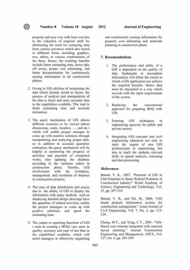
Journal of Engineering Volume 18 August 2012 Number 8
985
properly and easy way with least cost due to the reduction of required staff, by eliminating the need for extracting data from various resources which also stored in different forms including graphics, text, tables, or various combinations of the three. Hence, the resulting benefits include faster estimating time, fewer take off errors, proper cost estimating, and better documentation for continuously reusing information in all construction phases.
2. Owing to GIS abilities of integrating the data which already stored as layers, the process of analysis and manipulation of the data is faster and more accurate than in the capabilities available. This lead to faster estimating time and accurate estimation.
3. The query mechanism of GIS allows
different scenarios to be viewed (about dimensions, codes, location, …, and etc.) which will enable project manager to come up with positive solutions through manipulating and analyzing proper data, so in addition to accurate quantities estimation, the query mechanism will be helpful in monitoring the progress of activities and payment of completed works, also updating the database according to the variation orders in construction phase. Thereby, GIS involvement with the avoidance, management, and resolution of disputes in construction projects.
4. The ease of data distribution and access due to the ability of GIS to display the information with many methods such as displaying detailed design drawings have the quantities of related activities, enable the project managers to come up with positive solutions, and speed the estimating time.
5. The output or reporting functions of GIS
( such as creating a BOQ) vary more in quality, accuracy and ease of use than in the capabilities available, which will assist managers in effectively organizing
and continuously reusing information for properly cost estimating and materials planning in construction phase.
7. Recomendations 1. The performance and utility of a
GIS is dependent on the quality of data. Inadequate or incomplete information will dilute the extent to which a GIS application can achieve the required benefits. Hence data must be structured in a way which accords with the input requirements of the system.
2. Replacing the conventional
approach for preparing BOQ with GIS.
3. Entering GIS techniques in
engineering agencies for public and private sectors.
4. Integrating GIS concepts into civil
engineering education not only to meet the urgent of non GIS professionals in engineering, but also to teach the students relevant skills in spatial analysis, reasoning and data processing.
References Bansal, V. K., 2007, “Potential of GIS to Find Solutions to Space Related Problems in Construction Industry” World Academy of Science, Engineering and Technology, Vol. 32, pp. 307-310. Bansal, V. K., and Pal, M., 2006, “GIS based projects information system for construction management.” Asian Journal of Civil Engineering, Vol. 7, No. 2, pp. 115-124. Cheng, M.Y., and Yang, C.Y., 2001, “GIS-Based cost estimate integrated with material layout planning.” Journal Construction Engineering and Management, ASCE, Vol. 127, No. 4, pp. 291-299.

Dr. Sedki Esmaeel Rezouki Application Of Geographic Information System For Ruqaya Hadi Rasheed Preparing The Bill Of Quantities Of Construction
Projects
986
6.Cheng, M.Y., and Yang, C.Y., 2001, “GIS-Based cost estimate integrated with material layout planning.” Journal Construction Engineering and Management, ASCE, Vol. 127, No. 4, pp. 291-299. Camp, C.V., and Brown, M.C., 1993, “GIS procedure for developing three dimensional subsurface profile.” Journal of Computing in Civil Engineering, ASCE, Vol. 7, No.3, pp. 296-309. Joshphar Kunapo, Ganeswara Rao Dasari, Kok-Kwang Phoon, and Thiam-Soon Tan, 2005, “Development of a Web-GIS Based Geotechnical Information System” Journal of Computing in Civil Engineering, ASCE, Vol. 19, No. 3, pp.323-327 Mohamed N. Jeljeli, Jeffrey S. Russell, Guy Meyer, H. W., and Alan P. Vonderohe, 1993, “Potential Application of Geographic Information System to Construction Industry” Journal of Construction Engineering and Management, ASCE, Vol. 119, No. 1, pp. 72-86.
Oloufa , A.R., Eltahan , A.A., and Papacostas, C.S., 1994, “Integrated GIS for construction site investigation.” Journal Construction Engineering and Management, ASCE, Vol. 120, No.1, pp. 211-222. Parsons, R. L., and Frost, J. D., 2000, “Intractive Analysis of Spatial Subsurface Data Using GIS-Based Tool” Journal of Computing in Civil Engineering, ASCE, Vol. 14, No. 4, pp.215-222. Sebt, M. H., Parvaresh Karan, E., and, Delavar, M. R., 2008, “Potential Application of GIS to Layout of Construction Temporary Facilities” International Journal of Civil Engineering, Vol. 6, No. 4, pp. 235-245.
Stephen E. Poku and David Arditi, 2006, “Construction Scheduling and Progress Control Using Geographical Information Systems” Journal of Computing in Civil Engineering, ASCE, Vol. 20, No. 5, pp.351-36o .
Construction Management Committee of the ASCE Construction Division. 1991, "Constructability and constructability program" Journal Construction Engineering and Management, ASCE, Vol. 17, No.1 pp.67-89.
Varghese, K., and O’Connor, J.T., 1995, “Routing large vehicles on industrial construction site.” Journal Construction Engineering and Management, ASCE, Vol. 121, No.1, pp. 1-12. Zhong, D., Zhu, J. Li, H., and Song, L., 2004, “Geographic information system based visual simulation methodology and its application in concrete dam construction processes.” Journal Construction Engineering and Management, ASCE, Vol. 130, No.5, pp. 742-750. List Of Symbols
BOQ Bills of Quantities
CAD Computer-Aided Drafting
RDBMS Relational Database Management System
GeoInfoSys Geotechnical Information System
TFs Temporary Facilities
DBMSs Database Management Systems
3D Three-Dimensional
GVSS GIS-Based Visual Simulation System
P3 Primavera Project Planner
ID Identification Descriptor
WBS Work Break Structure
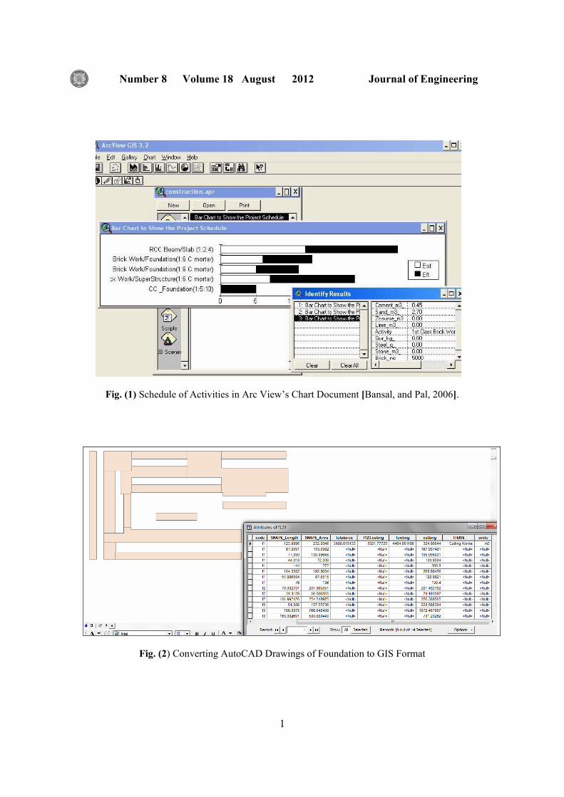
Journal of Engineering Volume 18 August 2012 Number 8
1
Fig. (1) Schedule of Activities in Arc View’s Chart Document [Bansal, and Pal, 2006].
Fig. (2) Converting AutoCAD Drawings of Foundation to GIS Format

Dr. Sedki Esmaeel Rezouki Application Of Geographic Information System For Ruqaya Hadi Rasheed Preparing The Bill Of Quantities Of Construction
Projects
988
Table (1) Comparison the BOQ of Tender, Site, and GIS
Item Unit BOQ
(Tender)Site GIS
1 Excavations Works m³ 4000 5060.1 5021.78
2 Subbase m³ 3000 2188.93 2181.44
3 Chlorofet m² 4000 4101.1 4102.23
4 Blinding m² 4000 3528.44 3532.92
5 RC of Foundations m³ 2300 2550.8 2550.89
6 Rc of Pedestals m³ 100 89.7 89.23
7 RC of Interior Tie Beams m³ 110 170 167.43
8 RC of Exterior Tie Beams m³ 120 91.2 90.8
9 RC of Columns m³ 500 336.84 366.8
10 RC of Beams m³ 1400 1197.5 1203.34
11 RC of Parapets m³ 150 125.3 121.56
12 RC of Slab m³ 1000 1190.4 1182.47
13 Bricks m³ _ 110.69 115.12
14 RC of Stair m³ _ 11.2 11.081

8العدد
18المجلد
اب
2012

August
2012 Number 8
Volume 18

College of Engineering Baghdad University Baghdad
List of Contents English Section: Page
The Effect of Different Types of Aggregate and Additives on the Properties of Self-Compacting Lightweight Concrete
Qusay Jar-Allah Hachim Prof. Dr. Nada M. Fawzi
875 - 888
Effect of Fire Flame (High Temperature) on the Behaviour of Axially loaded Reinforced SCC Short Columns
Amer F. Izzat
889 - 904
Development A Method For Production Of Carbon Nanotubes
Dr. Mohamed. I. M Dr. N. J .Saleh L. H. Mohmood.
905 - 913
Spectral Technique for Baud Time Estimation
Mohammed K. Al-Haddad Dr. Sarcout N. Abdullah Prof. Qais S. Ismail.
914 - 923
The Effect Of Laminated Layers On The Flutter Speed Of Composite Wing
Asst. Prof. Dr.Ahmed Abd Al-Hussain Ali Mohammed Ismael Hamed
924 - 934
Study the Effect of Ceramic Coating on the Performance and Emissions of Diesel Engine
Dr. Ibtihal Al-Namie Dr. Mahmoud A. Mashkour Ahmed Sabah Hameed
935 - 942
The Effect Of Variable Load On Dynamic Behavior Of Thin Pipe By Hamilton Principle And Cfx-Ansys
Assist Lecturer Ali Fahad Fahem
943 - 960
Buckling Analysis Of Damaged Composite Plates Under Uniform Or Non-Uniform Compressive Load
Prof. Dr. Adnan Naji Jameel Kawther Khalid Younus
961 - 978

Application of Geographic Information System for Preparing the Bill of Quantities of Construction Projects Asst. Prof. Dr. Sedki Esmaeel Rezouki Ruqaya Hadi Rashee
979 - 988

المحتويات قائمة
:القسم العربي
الصفحة العنوان 159 – 151 اتخاذ القرارات ذات الدوال الكسرية باستخدام طريقة برمجة األهداف
م واثق حياوي اليذ.م